A Dynamic Data Structure for Flexible Molecular Maintenance and Informatics ∗ Chandrajit Bajaj Institute for Computational Engineering and Science University of Texas Austin, TX 78712 [email protected]Rezaul Alam Chowdhury Institute for Computational Engineering and Science University of Texas Austin, TX 78712 [email protected]Muhibur Rasheed Institute for Computational Engineering and Science University of Texas Austin, TX 78712 [email protected]ABSTRACT We present the “Dynamic Packing Grid” (DPG) data struc- ture along with details of our implementation and perfor- mance results, for maintaining and manipulating flexible molecular models and assemblies. DPG can efficiently main- tain the molecular surface (e.g., van der Waals surface and the solvent contact surface) under insertion/deletion/ move- ment (i.e., updates) of atoms or groups of atoms. DPG also permits the fast estimation of important molecular prop- erties (e.g., surface area, volume, polarization energy, etc.) that are needed for computing binding affinities in drug de- sign or in molecular dynamics calculations. DPG can addi- tionally be utilized in efficiently maintaining multiple “rigid” domains of dynamic flexible molecules. In DPG, each up- date takes only O (log w) time w.h.p. on a RAM with w-bit words i.e., O (1) time in practice, and hence is extremely fast. DPG’s queries include the reporting of all atoms within O (rmax) distance from any given atom center or point in 3- space in O (log log w) (= O (1)) time w.h.p., where rmax is the radius of the largest atom in the molecule. It can also answer whether a given atom is exposed or buried under the surface within the same time bound, and can return the entire molecular surface in O (m) worst-case time, where m is the number of atoms on the surface. The data structure uses space linear in the number of atoms in the molecule. Categories and Subject Descriptors I.3.5 [Computer Graphics]: Computational Geometry and Object Modeling—boundary representations; curve, surface, solid, and object representations; geometric algorithms, lan- guages, and systems; physically based modeling ; F.2.2 [Analysis of Algorithms and Problem Complexity]: Nonnumeri- cal Algorithms and Problems—computations on discrete struc- ∗ This research was supported in part by NSF grant CNS- 0540033 and NIH contracts R01-EB00487, R01-GM074258, R01-GM07308. Permission to make digital or hard copies of all or part of this work for personal or classroom use is granted without fee provided that copies are not made or distributed for profit or commercial advantage and that copies bear this notice and the full citation on the first page. To copy otherwise, to republish, to post on servers or to redistribute to lists, requires prior specific permission and/or a fee. SIAM/ACM Joint Conference on Geometric and Physical Modeling 2009 San Francisco, California USA Copyright 200X ACM X-XXXXX-XX-X/XX/XX ...$5.00. tures; geometrical problems and computations ; J.6 [Computer- Aided Engineering]: Computer-aided design (CAD) General Terms Algorithms, Design, Performance Keywords shape modeling, de novo drug design, computer aided de- sign, interactive software, protein folding, molecular docking 1. INTRODUCTION Many human functional processes are mediated through the interactions amongst proteins, a major molecular con- stituent of our anatomical makeup. A computational under- standing of these interactions provides important clues for developing therapeutic interventions related to diseases such as cancer and metabolic disorders. Computational meth- ods such as automated docking through shape and energetic complementarity scoring, aim to gain insight and predict such molecular interactions. The most common model for proteins is a collection of atoms represented by spherical balls, with radii equal to their van der Waals radii [35, 16]. The surface of the union of these spheres is known as the van der Waals surface. Lee and Richards introduced the concept of accessibility to the sol- vent [31]. Proteins are not isolated, but commonly present in solutions, especially water. Also, the van der Waals sur- face contains too many internal atoms and patches which are not accessible by the solvent or any other protein that may bind to it. Hence, Lee and Richards gave a new defi- nition for the protein surface or protein-solvent interface as the surface accessible to the watery solvent. They modeled water molecules as spheres with radius 1.4 ˚ A, and considered the locus of the center of one such ‘probe’, as it rolled along the protein surface as the Solvent Accessible Surface (SAS). Richards then gave a more commonly used definition for molecular surface as a set of contact and reentrant patches [42]. Though Connolly considered this an alternative defini- tion of the SAS surface in [13], now it is commonly known as the Solvent Contact Surface (SCS), or Solvent Excluded Surface (SES) or simply the molecular surface/interface of the protein. Protein interactions or protein-protein docking involves induced complementary fit between flexible protein inter- faces and additionally the interface conformational changes are often critical during the lock and key matching [43].
Transcript
A Dynamic Data Structure for Flexible MolecularMaintenance and Informatics ∗
Chandrajit BajajInstitute for ComputationalEngineering and Science
ABSTRACTWe present the “Dynamic Packing Grid” (DPG) data struc-ture along with details of our implementation and perfor-mance results, for maintaining and manipulating flexiblemolecular models and assemblies. DPG can efficiently main-tain the molecular surface (e.g., van der Waals surface andthe solvent contact surface) under insertion/deletion/ move-ment (i.e., updates) of atoms or groups of atoms. DPG alsopermits the fast estimation of important molecular prop-erties (e.g., surface area, volume, polarization energy, etc.)that are needed for computing binding affinities in drug de-sign or in molecular dynamics calculations. DPG can addi-tionally be utilized in efficiently maintaining multiple “rigid”domains of dynamic flexible molecules. In DPG, each up-date takes only O (log w) time w.h.p. on a RAM with w-bitwords i.e., O (1) time in practice, and hence is extremelyfast. DPG’s queries include the reporting of all atoms withinO (rmax) distance from any given atom center or point in 3-space in O (log log w) (= O (1)) time w.h.p., where rmax isthe radius of the largest atom in the molecule. It can alsoanswer whether a given atom is exposed or buried underthe surface within the same time bound, and can return theentire molecular surface in O (m) worst-case time, where mis the number of atoms on the surface. The data structureuses space linear in the number of atoms in the molecule.
Categories and Subject DescriptorsI.3.5 [Computer Graphics]: Computational Geometry andObject Modeling—boundary representations; curve, surface,solid, and object representations; geometric algorithms, lan-guages, and systems; physically based modeling ; F.2.2 [Analysisof Algorithms and Problem Complexity]: Nonnumeri-cal Algorithms and Problems—computations on discrete struc-
∗This research was supported in part by NSF grant CNS-0540033 and NIH contracts R01-EB00487, R01-GM074258,R01-GM07308.
Permission to make digital or hard copies of all or part of this work forpersonal or classroom use is granted without fee provided that copies arenot made or distributed for profit or commercial advantage and that copiesbear this notice and the full citation on the first page. To copy otherwise, torepublish, to post on servers or to redistribute to lists, requires prior specificpermission and/or a fee.SIAM/ACM Joint Conference on Geometric and Physical Modeling 2009San Francisco, California USACopyright 200X ACM X-XXXXX-XX-X/XX/XX ...$5.00.
Keywordsshape modeling, de novo drug design, computer aided de-sign, interactive software, protein folding, molecular docking
1. INTRODUCTIONMany human functional processes are mediated through
the interactions amongst proteins, a major molecular con-stituent of our anatomical makeup. A computational under-standing of these interactions provides important clues fordeveloping therapeutic interventions related to diseases suchas cancer and metabolic disorders. Computational meth-ods such as automated docking through shape and energeticcomplementarity scoring, aim to gain insight and predictsuch molecular interactions.
The most common model for proteins is a collection ofatoms represented by spherical balls, with radii equal totheir van der Waals radii [35, 16]. The surface of the union ofthese spheres is known as the van der Waals surface. Lee andRichards introduced the concept of accessibility to the sol-vent [31]. Proteins are not isolated, but commonly presentin solutions, especially water. Also, the van der Waals sur-face contains too many internal atoms and patches whichare not accessible by the solvent or any other protein thatmay bind to it. Hence, Lee and Richards gave a new defi-nition for the protein surface or protein-solvent interface asthe surface accessible to the watery solvent. They modeledwater molecules as spheres with radius 1.4A, and consideredthe locus of the center of one such ‘probe’, as it rolled alongthe protein surface as the Solvent Accessible Surface (SAS).Richards then gave a more commonly used definition formolecular surface as a set of contact and reentrant patches[42]. Though Connolly considered this an alternative defini-tion of the SAS surface in [13], now it is commonly knownas the Solvent Contact Surface (SCS), or Solvent ExcludedSurface (SES) or simply the molecular surface/interface ofthe protein.
Protein interactions or protein-protein docking involvesinduced complementary fit between flexible protein inter-faces and additionally the interface conformational changesare often critical during the lock and key matching [43].
Figure 1: Visualization of the Rice Dwarf Virus (RDV) nucleo-capsid contains 3.5 million atoms (left) whileMicrotubule contains 1.2 million (right), using TexMol (http://cvcweb.ices.utexas.edu/software/#TexMol).In this figure, atoms are color-coded using the standard Corey, Pauling, Koltun (CPK) color scheme.
The flexible docking solution space consisting of all relativepositions, orientations and conformations of the proteins,is searched, and the putative dockings are evaluated us-ing combinations of interface complementarity scoring, andatomic pair-wise charged Coulombic interactions [27]. Sinceproteins function in their predominantly watery (solvent)environment, the computation of protein solvation energy(or known as protein - solvent interaction energy) also playsan important role in determining inter-molecular bindingaffinities “in-vivo” for drug screening, as well as in moleculardynamics simulations [52], and in the study of hydropho-bicity and protein folding. When computing the solvationenergy for molecules, it is crucial to correctly model andsample the protein - solvent interface.
Since Richards introduced the SES definition, a numberof techniques have been devised for static construction ofthe molecular surface (e.g., [12, 13, 53, 17, 50, 3, 45, 44, 55,23, 7, 6]). However, not much work has been done on dy-namic maintenance of molecular surfaces. In [8] Bajaj et al.considered limited dynamic maintenance of molecular sur-faces based on Non Uniform Rational BSplines ( NURBS )descriptions for the patches. Eyal and Halperin [19, 20] pre-sented an algorithm based on dynamic graph connectivitythat updates the molecular surface after a conformationalchange in O
`log2 n
´amortized time per affected (by this
change) atom.In this paper we present the Dynamic Packing Grid (DPG)
– a space and time efficient data structure that maintainsa collection of balls (atoms) in 3-space allowing a range ofspherical range queries and updates for rapid scoring of flex-ible protein-protein interactions. The efficiency of the datastructure results from the assumption that the centers of twodifferent balls in the collection cannot come arbitrarily closeto each other, which is a natural property of molecules. Aconsequence of this assumption is that any ball in the collec-tion can intersect at most a constant number of other balls.On a RAM with w-bit words, the data structure can re-port all balls intersecting a given ball or within O (rmax)distance from a given point in O (log log w) time w.h.p.,where rmax is the radius of the largest ball in the collec-tion. It can also answer whether a given ball is exposed(i.e., lies on the union boundary) or buried within the sametime bound. At any time the entire union boundary canbe extracted from the data structure in O (m) time in theworst-case, where m is the number of atoms on the bound-
ary. Updates (i.e., insertion/deletion/movement of a ball)are supported in O (log w) time (w.h.p.). The data struc-ture uses linear space. A packing grid can maintain boththe van der Waals surface and the solvent contact surface(SCS) of a molecule within the performance bounds men-tioned above. Packing grids can be used to maintain the sur-face of a flexible molecule decomposed into rigid domains sothat applying a bending/shearing/twisting motion betweentwo domains takes O (1 + m log w) time (w.h.p.), where m isthe number of atoms in the connectors between the two do-mains. We also describe a Hierarchical Packing Grid (HPG)data structure that maintains a molecule at multiple resolu-tions (atomic and coarser) under updates, and can computeany mixed resolution surface efficiently. Packing grids canalso aid in fast energetics calculation by rapidly locating theatoms close to each sampled quadrature point on the SCS.
DPG has potential applications in interactive software toolsdeveloped for de novo drug design (e.g., [30, 46, 18, 29]),protein folding (e.g., [28, 14]) and molecular docking (e.g.,[33, 2]) that use human intuition and biological knowledgein order to steer the prediction process. These applica-tions often need to handle extremely large molecules andmacromolecules (e.g., as shown in Figure 1 Rice Dwarf Viruswith 3.5 million atoms, and Microtubule has 1.2 million),and need to perform a sequence of dynamic updates onthem in real time. The Molecule Evaluator [30, 18] is ade novo molecular design software based on adaptive inter-active evolution. In a series of interactive steps it appliesa set of problem-specific mutation (e.g., add/remove atom,add/remove group) and recombination operators on a setof evolving molecules, and keeps track of several chemicaland biological properties of each molecule (e.g., molecularmass, hydrophobicity, etc.). The ProteinShop software [28,14] allows the interactive creation of protein structures (e.g.,through shape manipulation) given an amino acid sequenceand a sequence of predicted secondary structure types foreach amino acid. DockingShop [33] is a successor of Pro-teinShop, which provides an interactive docking environ-ment with flexibility of side chains and backbone movement.Users can adjust the receptor protein structure by rotatingthe backbone dihedral angles, changing the dihedral anglesof selected residues, substituting the side chain of selectedresidues using a rotamer library, or changing a residue foranother while keeping the backbone fixed. Figure 2 shows anexample where the flexible movement/rearrangement of the
(a)
(b)
Figure 2: Figures (a) and (b) show the structure ofa soluble fragment of the envelope (E) Glycoproteinfrom DV (dengue virus) type 2. Figure (a) showsthe crystals grown in the presence (pre-fusion) ofthe detergent n-octyl-β-D-glucoside (β-OG, coloredin green), and Figure (b) shows the same in itsabsence (post-fusion). The key difference betweenthese two structures is a local rearrangement of the“kl” β-hairpin (residues 268-280) and the concomi-tant opening up of a hydrophobic pocket for ligandbinding. In Figure (a) this pocket is occupied by amolecule of β-OG [36].
“kl” β-hairpin on the envelope (E) Glycoprotein of denguevirus opens up a hydrophobic pocket for ligand binding, andthe inhibitor n-octyl-β-D-glucoside docks into that pocket.VRDD [2] supports molecular visualization and interactivedocking in a VR environment, and allows side-chain flexibil-ity.
The molecular dynamic simulation tool IMD [49] allowsinteractive manipulation of bio-molecular systems. It com-bines interactive molecular visualization (using VMD [26])with molecular dynamic simulation (using NAMD [38, 41])in the background that supports manipulation of moleculesby applying force to single atoms. Traditional all-atom molec-ular dynamics (MD) simulation reveals in detail the proteinfolding process, but it is restricted to small time scales onthe order of nanosecond [47] and small length range on theorder of nanometer [32, 34]. To fully investigate the foldingprocess of a protein into its functional structure, a largertimescale from micro- to millisecond and larger length scaleof micrometer are needed [4]. Protein coarse grained (CG)models which represent clusters of atoms with similar phys-ical properties by CG beads and simplify the interactionssignificantly reduce the size of the system and therefore be-come a promising approach to reproduce large-scale proteinmotions.
The DPG data structure also has potential applications intracking the dynamic structure of a particle system as parti-cles move, appear and disappear [5, 22, 25]. Particle systemsare used for modeling a number of physical world scenariosranging from cosmological systems and plasma physics to
molecular systems, where particles are defined as smoothfunctions with compact support. The applications are wideand varied and include chemistry, material science, and bio-engineering. The dynamic re-meshing problem for time de-pendent particle systems arise in gas hydrodynamics simula-tions essential in the computational investigation of the for-mation of large scale structures, such as galaxies and galaxyclusters, in the universe [25]. For the meshing of particlesystems, it suffices to consider particles as idealized balls, orradially symmetric domains of support of their kernels.
The rest of the paper is organized as follows. We describeand analyze the packing grid data structure in Section 2. Wegive some preliminaries in Section 2.1, describe the layout ofthe data structure in Section 2.2, and describe and analyzethe supported queries and updates in Section 2.3. In Sec-tion 3 we describe how to use packing grids for maintainingthe surface of a molecule decomposed into rigid domains,and in Section 4 we describe hierarchical packing grids formaintaining mixed resolution surfaces. In Section 5 we de-scribe some applications of packing grids. Our experimentalresults are included in Section 6.
2. THE DYNAMIC PACKING GRID DATASTRUCTURE
We describe the packing grid data structure for maintain-ing a set M of balls in 3-space efficiently under the followingset of queries and updates. By B = (c, r) we denote a ballwith center c and radius r.
Queries.
1. Intersect( c, r ): Return all balls in M that intersectthe given ball B = (c, r). The given ball may or maynot belong to the set M .
2. Range( p, δ ): Return all balls in M with centerswithin distance δ of point p. We assume that δ is atmost a constant multiple of the radius of the largestball in M .
3. Exposed( c, r ): Returns true if the ball B = (c, r)contributes to the outer boundary of the union of theballs in M . The given ball must belong to M .
4. Surface( ): Returns the outer boundary of the unionof the balls in M . If there are multiple disjoint outerboundary surfaces defined by M , the routine returnsany one of them.
Updates.
1. Add( c, r ): Add a new ball B = (c, r) to the set M .
2. Remove( c, r ): Remove the ball B = (c, r) from M .
3. Move( c1, c2, r ): Move the ball with center c1 andradius r to a new center c2.
We assume that at all times during the lifetime of the datastructure the following holds.
Assumption 2.1. If rmax is the radius of the largest ballin M , and dmin is the minimum Euclidean distance betweenthe centers of any two balls in M , then rmax = O (dmin).
In general, a ball in a collection of n balls in 3-space canintersect Θ (n) other balls in the worst case, and it has beenshown in [11] that the boundary defined by the union of theseballs has a worst-case combinatorial complexity of Θ
`n2
´.
Time Complexity
OperationsAssuming
tq = O (log log w),tu = O (log w)
Assumingtq = O (log log n),
tu = O“
log n
log log n
”
Range( p, δ ) | Intersect( c, r ) | Exposed( c, r )(δ = O (rmax))
O (log log w) (w.h.p.) O (log log n) (w.h.p.)
Surface( ) O (#balls on surface) (worst-case)
Add( c, r ) | Remove( c, r ) | Move( c1, c2, r ) O (log w) (w.h.p.) O“
log n
log log n
”(w.h.p.)
Assumptions: (i) RAM with w-bit Words, (ii) Collection of n Balls,and (iii) rmax = O (minimum distance between two balls)
Table 1: Time complexities of the operations supported by the packing grid data structure.
However, if M is a “union of balls” representation of theatoms in a molecule, then assumption 2.1 holds naturally[24, 51], and as proved in [24], in that case, both complexitiesimprove by a factor of n. The following theorem states theconsequences of the assumption.
Theorem 2.1. (Theorem 2.1 in [24], slightly modified)Let M = B1, . . . , Bn be a collection of n balls in 3-spacewith radii r1, . . . , rn and centers at c1, . . . , cn. Let rmax =maxi ri and let dmin = mini,j d(ci, cj), where d(ci, cj)is the Euclidean distance between ci and cj . Also let δM =δB1, . . . , δBn be the collection of spheres such that δBi isthe boundary surface of Bi. If rmax = O (dmin) (i.e., As-sumption 2.1 holds), then:
(i) Each Bi ∈ M intersects at most 216 · (rmax/dmin)3 =O (1) other balls in M .
(ii) The maximum combinatorial complexity of the bound-ary of the union of the balls in M is O
`(rmax/dmin)3 · n
´
= O (n).
Proof. Similar to the proof of Theorem 2.1 in [24].
Therefore, as Theorem 2.1 suggests, for intersection queriesand boundary construction, one should be able to handle Mmore efficiently if assumption 2.1 holds. The efficiency ofour data structure, too, partly depends on this assumption.
2.1 PreliminariesBefore we describe our data structure we present severaldefinitions in order to simplify the exposition.
Definition 2.1 (r-grid and grid-cell). An r-grid isan axis-parallel infinite grid structure in 3-space consistingof cells of size r×r×r (r ∈ R) with the root (i.e., the cornerwith the smallest x, y, z coordinates) of one of the cells co-inciding with origin of the (Cartesian) coordinate axes. Thegrid cell that has its root at Cartesian coordinates (ar, br, cr)(where a, b, c ∈ Z) is referred to as the (a, b, c, r)-cell or sim-ply as the (a, b, c)-cell when r is clear from the context.
Definition 2.2 (grid-line). The (b, c, r)-line (whereb, c ∈ Z) in an r-grid consists of all (x, y, z, r)-cells with yand z fixed to b and c, respectively. When r is clear from thecontext the (b, c, r)-line will simply be called the (b, c)-line.
Observe that each cell on the (b, c, r)-line can be identifiedwith a unique integer, e.g., the cell at index a ∈ Z on thegiven line corresponds to the (a, b, c, r)-cell in the r-grid.
Definition 2.3 (grid-plane). The (c, r)-plane (wherec ∈ Z) in an r-grid consists of all (x, y, z, r)-cells with z fixedto c. The (c, r)-plane will be referred to as the c-plane whenr is clear from the context.
The (c, r)-plane can be decomposed into an infinite numberof lines each identifiable with a unique integer. For example,index b ∈ Z uniquely identifies the (b, c, r)-line on the givenplane. Also each grid-plane in the r-grid can be identifiedwith a unique integer, e.g., the (c, r)-plane is identified by c.
The proof of the following lemma is straight-forward.
Lemma 2.1. Let M = B1, . . . , Bn be a collection of nballs in 3-space with radii r1, . . . , rn and centers at c1, . . . , cn.Let rmax = maxi ri and let dmin = mini,j d(ci, cj),where d(ci, cj) is the Euclidean distance between ci and cj .Suppose M is stored in the 2rmax-grid G. Then
(i) If rmax = O (dmin) (i.e., Assumption 2.1 holds) theneach grid-cell in G contains the centers of at most 64 ·(rmax/dmin)3 = O (1) balls in M .
(ii) Each ball in M intersects at most 8 grid-cells in G.
(iii) For a given ball B ∈ M with center in grid-cell C, thecenter of each ball intersecting B lies either in C or inone of the 26 grid-cells adjacent to C.
(iv) The number of non-empty (i.e., containing the centerof at least one ball in M) grid-cells in G is at mostn, and the same bound holds for grid-lines and grid-planes.
At the heart of our data structure is a fully dynamic onedimensional integer range reporting data structure for wordRAM described in [37]. The data structure in [37] main-tains a set S of integers under updates (i.e., insertions anddeletions), and answers queries of the form: report any orall points in S in a given interval. The following theoremsummarizes the performance bounds of the data structurewhich are of interest to us.
Theorem 2.2. (proved in [37]) On a RAM with w-bitwords the fully dynamic one dimensional integer range re-porting problem can be solved in linear space, and with highprobability bounds of O (tu) and O (tq + k) on update timeand query time, respectively, where k is the number of itemsreported, and
(i) tu = O (log w) and tq = O (log log w) using the datastructure in [37]; and
(ii) tu = O (log n/log log n) and tq = O (log log n) usingthe data structure in [37] for small w and a fusion tree[21] for large w.
The data structure can be augmented to store satellite in-formation of size O (1) with each integer without degradingits asymptotic performance bounds. Therefore, it supportsthe following three functions:
1. Insert( i, s ): Insert an integer i with satellite infor-mation s.
2. Delete( i ): Delete integer i from the data structure.
3. Query( l, h ): Return the set of all 〈 i, s 〉 tupleswith i ∈ [l, h] stored in the data structure.
2.2 Description (Layout) of the Packing GridData Structure
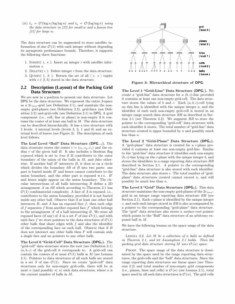
We are now in a position to present our data structure. LetDPG be the data structure. We represent the entire 3-spaceas a 2rmax-grid (see Definition 2.1), and maintain the non-empty grid-planes (see Definition 2.3), grid-lines (see Defi-nition 2.2) and grid-cells (see Definition 2.1) in DPG. A gridcomponent (i.e., cell, line or plane) is non-empty if it con-tains the center of at least one ball in M . The data structurecan be described hierarchically. It has a tree structure with5 levels: 4 internal levels (levels 3, 2, 1 and 0) and an ex-ternal level of leaves (see Figure 3). The description of eachlevel follows.
The Leaf Level “Ball” Data Structure (DPG−1). Thedata structure stores the center c = (cx, cy , cz) and the ra-dius r of the given ball B. It also includes a Boolean flagexposed which is set to true if B contributes to the outerboundary of the union of the balls in M , and false other-wise. If another ball B′ intersects B, it does so on a circlewhich divides the boundary δB of B into two parts: onepart is buried inside B′ and hence cannot contribute to theunion boundary, and the other part is exposed w.r.t. B′
and hence might appear on the union boundary. The cir-cular intersections of all balls intersecting B define a 2Darrangement A on δB which according to Theorem 2.1 hasO (1) combinatorial complexity. A face of A is exposed, i.e.,contributes to the union boundary, provided it is not buriedinside any other ball. Observe that if at least one other ballintersects B, and A has an exposed face f , then each edgeof f separates f from another exposed face f ′ which belongsto the arrangement A′ of a ball intersecting B. We store allexposed faces (if any) of A in a set F of size O (1), and witheach face f we store pointers to the data structures of O (1)other balls that share edges with f and also the identifierof the corresponding face on each ball. Observe that if Bdoes not intersect any other balls then F will contain onlya single face and no pointers to any other balls.
The Level 0 “Grid-Cell”Data Structure (DPG0). The“grid-cell” data structure stores the root (see Definition 2.1)(a, b, c) of the grid-cell it corresponds to. A grid-cell cancontain the centers of at most O (1) balls in M (see Lemma2.1). Pointers to data structures of all such balls are storedin a set S of size O (1). Since we create “grid-cell” datastructures only for non-empty grid-cells, there will be atmost n (and possibly ≪ n) such data structures, where n isthe current number of balls in M .
Figure 3: Hierarchical structure of DPG.
The Level 1 “Grid-Line” Data Structure (DPG1). Wecreate a “grid-line” data structure for a (b, c)-line providedit contains at least one non-empty grid-cell. The data struc-ture stores the values of b and c. Each (a, b, c)-cell lyingon this line is identified with the unique integer a, and theidentifier of each such non-empty grid-cell is stored in aninteger range search data structure RR as described in Sec-tion 2.1 (see Theorem 2.2). We augment RR to store thepointer to the corresponding “grid-cell” data structure witheach identifier it stores. The total number of “grid-line”datastructure created is upper bounded by n and possibly muchless than n.
The Level 2 “Grid-Plane” Data Structure (DPG2).A “grid-plane” data structure is created for a c-plane pro-vided it contains at least one non-empty grid-line. Similarto the “grid-line” data structure it identifies each non-empty(b, c)-line lying on the c-plane with the unique integer b, andstores the identifiers in a range reporting data structure RRdescribed in Section 2.1. A pointer to the corresponding“grid-line” data structure is also stored with each identifier.The data structure also stores c. The total number of “grid-plane” data structures created cannot exceed n, and willpossibly be much less than n.
The Level 3 “Grid”Data Structure (DPG3). This datastructure maintains the non-empty grid-planes of the 2rmax-grid in an integer range reporting data structure RR (seeSection 2.1). Each c-plane is identified by the unique integerc, and each such integer stored in RR is also accompanied bya pointer to the corresponding “grid-plane” data structure.The “grid” data structure also stores a surface-root pointerwhich points to the “Ball” data structure of an arbitrary ex-posed ball in M .
We have the following lemma on the space usage of the datastructure.
Lemma 2.2. Let M be a collection of n balls as definedin Theorem 2.1, and let Assumption 2.1 holds. Then thepacking grid data structure storing M uses O (n) space.
Proof. The space usage of the data structure is domi-nated by the space used by the range reporting data struc-tures, the grid-cells and the “ball” data structures. Since therange reporting data structures use linear space (see Theo-rem 2.2) and total number of non-empty grid components(i.e., planes, lines and cells) is O (n) (see Lemma 2.1), totalspace used by all such data structures is O (n). The grid cells
contain pointers to “ball” data structures, and since no twogrid-cells point to the same “ball” data structure, total spaceused by all grid-cells is also O (n). Each “ball” data struc-ture contains the arrangement A and the face decompositionF of the exposed (if any) faces of the ball. The total spaceneeded to store all such arrangements and decompositionsis O
`(rmax/dmin)3 · n
´(see Theorem 2.1) which reduces to
O (n) under Assumption 2.1. Thus the total space used bythe data structure is O (n).
2.3 Queries and UpdatesThe queries and updates supported by the data structureare implemented as follows.
2.3.1 Queries.
(1) Range( p, δ ): Let p = (px, py, pz). We perform thefollowing steps.
i. Level 3 Range Query: We invoke the functionQuery( l, h ) of the range reporting data structureRR under DPG3 (i.e., the level 3 “grid” data structure)with l = ⌊(pz − δ)/(2rmax)⌋ and h = ⌊(pz + δ)/(2rmax)⌋.This query returns a set S2 of tuples, where each tuple〈 c, Pc 〉 ∈ S2 refers to a non-empty c-plane with apointer Pc to its level 2 “grid-plane” data structure.
ii. Level 2 Range Query: For each 〈 c, Pc 〉 ∈ S2, wecall the range query function under the correspondinglevel 2 data structure with l = ⌊(py − δ′)/(2rmax)⌋ andh = ⌊(py + δ′)/(2rmax)⌋, where (δ′)2 = δ2 − (c − pz)
2
if c − pz < δ, and δ′ = rmax otherwise. This query re-turns a set S1,c of triples, where each triple 〈 b, c, Pb,c 〉 ∈S1,c refers to a non-empty ( b, c )-line with a pointerPb,c to its level 1 “grid-line” data structure. We obtainthe set S1 by merging all S1,c sets.
iii. Level 1 Range Query: For each 〈 b, c, Pb,c 〉 ∈ S1,we call the integer range query function under thecorresponding level 1 “grid-line” data structure withl = ⌊(px − δ′′)/(2rmax)⌋ and h = ⌊(px + δ′′)/(2rmax)⌋,where (δ′′)2 = δ2−(b − py)2−(c − pz)
2 if δ2 > (b − py)2+(c − pz)
2, and δ′′ = rmax otherwise. This query re-turns a set S0,b,c of quadruples, where each quadru-ples 〈 a, b, c, Pa,b,c 〉 ∈ S0,b,c refers to a non-empty( a, b, c )-cell with a pointer Pa,b,c to its level 0 “grid-cell” data structure. We obtain the set S0 by mergingall S0,b,c sets.
iv. Ball Collection: For each 〈 a, b, c, Pa,b,c 〉 ∈ S0,we collect from the level 0 data structure of the cor-responding ( a, b, c )-cell each ball whose center lieswithin distance δ from p. We collect the pointer to theleaf level “ball” data structure of each such ball in aset S, and return this set.
The correctness of the function follows trivially since it queriesa region in 3-space which includes the region covered bya ball of radius δ centered at p. It is straight-forward tosee that the function makes at most O
`π · (⌈δ/rmax⌉ + 1)2
´
calls to a range reporting data structure, and collects ballsfrom at most O
`43π · (⌈δ/rmax⌉ + 1)3
´grid-cells. Using Lemma
2.1 and Theorem 2.2, we conclude that w.h.p. the func-tion terminates in O
`(δ/rmax)2 · tq + ((δ + rmax)/dmin)3
´
time. Assuming rmax = O (dmin) (i.e., Assumption 2.1)and δ = O (rmax), the complexity reduces to O (tq) (w.h.p.).
(2) Intersect( c, r ): Let B = (c, r) be the given ball. Weperform the following two steps.
i. Ball Collection: We call Range( c, r + rmax ) andcollect the output in set S which contains pointers tothe data structure of each ball in M with its centerwithin distance r + rmax from c.
ii. Identifying Intersecting Balls: From S we removethe data structure of each ball that does not intersectB, and return the resulting (possibly reduced) set.
We know from elementary geometry that two balls of radiir1 and r2 cannot intersect unless their centers lie within dis-tance r1 + r2 of each other. Therefore, step (i) correctlyidentifies all balls that can possibly intersect B, and step(ii) completes the identification. Step (i) takesO
`tq + (rmax/dmin)3
´time w.h.p., and step (ii) terminates
in O`(rmax/dmin)3
´time in the worst case. Therefore, un-
der Assumption 2.1 w.h.p. this function runs in O (tq) time.
(3) Exposed( c, r ): Let B = (c, r) be the given ball. Welocate B’s data structure by calling Range( c, 0 ), andreturn the value stored in its exposed field. Clearly, thefunction takes O
`tq + (rmax/dmin)3
´time (w.h.p.) which
reduces to O (tq) (w.h.p.) under Assumption 2.1.
(4) Surface( ): The surface-root pointer under the level3 “grid” data structure points to the “ball” data structureof a ball B on the union boundary of M . We scan the setF of exposed faces of B, and using the pointers to otherexposed balls stored in F we perform a depth-first traversalof all exposed balls in M and return the exposed faces oneach such ball. Let m be the number of balls contributingto the union boundary of M . Then according to Theorem2.1 the depth-first search takes O
`(rmax/dmin)3 · m
´time
in the worst case which reduces to O (m) under Assumption2.1.
2.3.2 Updates.
(1) Add( c, r ): Let c = (cx, cy, cz) and let c′u =j
cu
2rmax
k,
where u ∈ x, y, z. We perform the following steps.
i. If M 6= ∅, let G be the grid data structure, otherwisecreate and initialize G. Add input ball to M .
ii. Query the range reporting data structure G.RR to lo-cate the data structure P for the c′z-plane. If P doesnot exist create and initialize P , and insert c′z alongwith a pointer to P into G.RR.
iii. Query P.RR and locate the data structure L for the(c′y, c′z)-line. If L does not exist then create and ini-tialize L, and insert c′y along with a pointer to L intoP.RR.
iv. Locate the data structure C for the (c′x, c′y, c′z)-cell byquerying L.RR. Create and initialize C if it does notalready exist, and insert c′x and a pointer to C intoL.RR.
v. Create and initialize a data structure B for the inputball and add it to the set C.S.
vi. Call Intersect( c, r ) and find the set I of the “ball”data structures of all balls that intersect the input ball.Create the arrangement B.A using the balls in I . Thenew ball may partly or fully bury some of the balls itintersects, and hence we need to update the arrange-ment B′.A, the set B′.F and the flag B′.exposed ofeach B′ ∈ I . The set B.F is created and B.exposed isinitialized using the information in the updated datastructures in I . If the surface-root pointer was point-ing to a ball in I that got completely buried by thenew ball, we update it to point to B instead.
Observe that the introduction of a new ball may affect thesurface exposure of only the balls it intersects (i.e., burysome/all of them partly or completely), and no other balls.Hence, the updates performed in step (vi) (in addition tothose in earlier steps) are sufficient to maintain the correct-ness of the entire data structure.
Steps (i) and (v) take O (1) time in the worst case, andw.h.p. each of steps (ii), (iii) and (iv) takes O (tq + tu)time. Finding the intersecting balls in step (vi) takesO
`tq + (rmax/dmin)3
´time w.h.p., according to Theorem
2.1 creating and updating the arrangements and faces willtake O
`(rmax/dmin)3 × (rmax/dmin)3
´= O
`(rmax/dmin)6
´
time (w.h.p.). Thus the Add function terminates inO
`tq + tu + (rmax/dmin)6
´time w.h.p., which reduces to
O (tu) (w.h.p.) assuming rmax = O (dmin) (i.e., Assump-tion 2.1).
(2) Remove( c, r ): This function is symmetric to theAdd function, and has exactly the same asymptotic timecomplexity. Hence, we do not describe it here.
(3) Move( c1, c2, r ): This function is implemented inthe obvious way by calling Remove( c1, r ) followed byAdd( c2, r ). It has the same asymptotic complexity as thetwo functions above.
Therefore, we have the following theorem.
Theorem 2.3. Let M be a collection of n balls in 3-spaceas defined in Theorem 2.1, and let Assumption 2.1 holds. Lettq and tu be as defined in Theorem 2.2. Then the packinggrid data structure storing M on a word RAM:
(i) uses O (n) space;
(ii) supports updates (i.e., insertion/deletion/movement ofa ball) in O (tu) time w.h.p.;
(iii) reports all balls intersecting a given ball or within O (rmax)distance from a given point in O (tq) time w.h.p., wherermax is the radius of the largest ball in M ; and
(iv) reports whether a given ball is exposed or buried inO (tq) time w.h.p., and returns the entire outer unionboundary of M in O (m) worst-case time, where m isthe number of balls on the boundary.
In Table 1 we list the time complexities of the operationssupported by our data structure.
3. EFFICIENT MAINTENANCE OF FLEX-IBLE MOLECULES UNDER DOMAIN MO-TIONS
Suppose we are given a flexible molecule decomposed intoseveral (mostly) rigid domains which interact either throughconnected chain segments or large interfaces. We refer tothese chain segments and interfaces as connectors. Domainsmay move with respect to each other through motions ap-plied to the connectors. Two domains connected by at leastone connector may undergo bending motion applied to somehinge point around some hinge axis. If they are connectedby only one connector, a twisting motion can also be ap-plied to the connector by updating torsion angles along itsbackbone. If two domains share a large interface area theymay undergo a shearing motion with respect to each other.However, though domains are mostly rigid they may haveflexible loops and side-chains on their surfaces.
We maintain a separate packing grid data structure Pi foreach domain Di. If two domains Di and Dj are connectedand i < j, the set Sij of all connectors between these twodomains are included in Pi, and a transformation matrixMij is kept with Pi that describes the exact location andorientation of the grid structure of Pj with respect to thatof Pi. Whenever some motion is applied to the connectorsin Sij , we update Pi in order to reflect the changes in thelocations of the atoms in these connectors, and also updateMij in order to reflect the new relative position and orienta-tion of Pj with respect to Pi. Hence such an update requiresO (1 + mij log w) time (w.h.p.), where mij is the number ofatoms in the connectors in Sij . We defer the tests to checkwhether any two domains intersect due to these movementsuntil we need to construct the surface of the entire moleculein response to a surface query. At that point we extract thesurface atoms from each Pi and insert them into an initiallyempty packing grid data structure P after applying neces-sary transformations. Thus generating the surface of theentire molecule requires O ( bm log w) time (w.h.p.), where bmis the sum of the number of atoms on the surface of eachdomain. If we need to update the conformation of a flexi-ble loop or a side-chain on the surface of some domain Di,we directly update the locations of the atoms affected bythis change in Pi. Such an update requires O ( em log w) time(w.h.p.), where em is the number of atoms affected. There-fore, we have the following lemma.
Lemma 3.1. The surface of a flexible molecule decom-posed into (mostly) rigid domains can be maintained usingpacking grid data structures so that
(i) updating for a bending/shearing/twisting motion ap-plied between two domains takes O (1 + m log w) time(w.h.p.), where m is the number of atoms in the con-nectors between the two domains;
(ii) updating the conformation of a flexible loop or a side-chain on the surface of a domain takes O ( em log w)time (w.h.p.), where em is the number of atoms affectedby this change; and
(iii) generating the surface of the entire molecule requiresO ( bm log w) time (w.h.p.), where bm is the sum of thenumber of atoms on the surface of each domain.
We construct a k-level hierarchical packing grid data struc-ture HPG(k) as follows. For i ∈ [0, k − 1], level i con-
tains a packing grid data structure DPG(i) with parameters
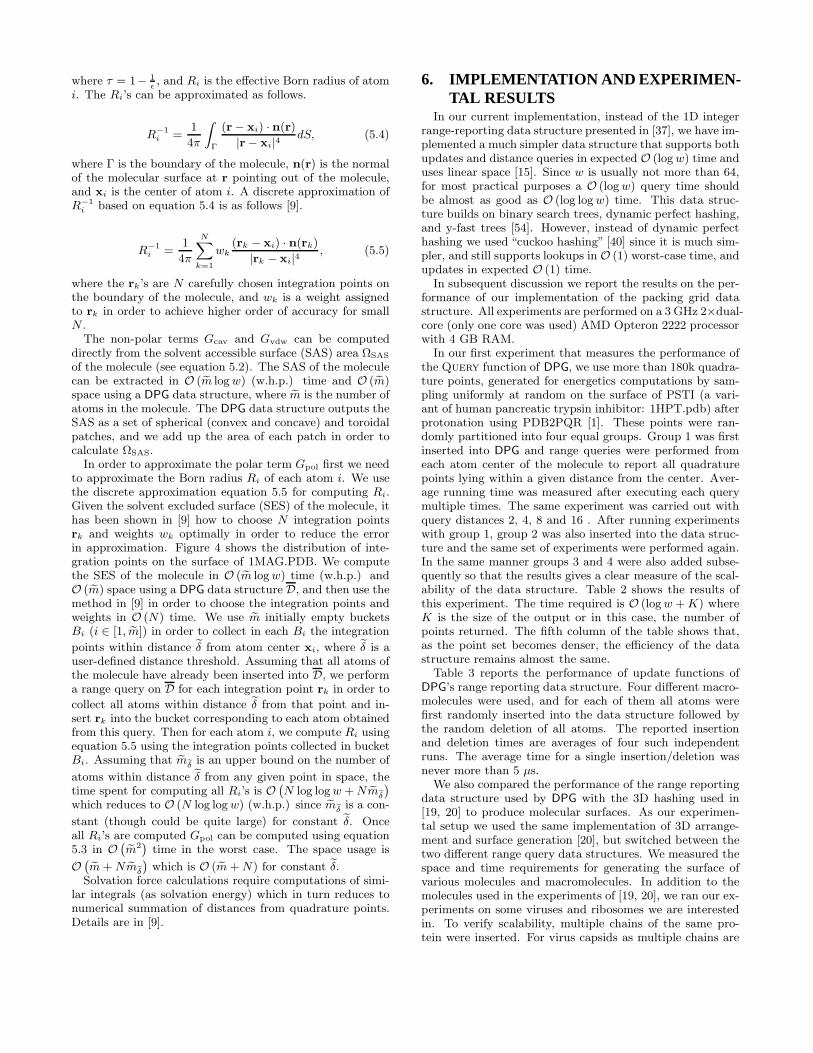
Figure 4: (LEFT) Gaussian integration points on the surface of peptide antibiotic Gramicidin A (1MAG).The surface is partitioned into 30,624 triangular patches, and there are three Gaussian quadrature nodes pertriangle. The nodes are then mapped onto the ASMS to form the red point cloud. (RIGHT) Electrostaticsolvation force computation for Gramicidin A. Atoms with the greatest electrostatic solvation force (top 5%)are colored in red; atoms having the weakest electrostatic solvation force (bottom 5%) are colored in blue.
〈r(i)max, d
(i)min〉 for which Assumption 2.1 holds. We also as-
sume that for i ∈ [0, k − 2], r(i+1)max = Θ
“r(i)max
”and d
(i+1)min =
Θ“d(i)min
”. The level 0 data structure DPG
(0) contains the
atomic level union of balls representation of the given moleculeM . For i ∈ [1, k − 1], DPG
(i) contains a coarser represen-
tation of the molecule represented in DPG(i−1). Each ball
in DPG(i) represents a grouping several neighboring balls
in DPG(i−1). A single doubly linked list links the parent
ball in DPG(i) to all its child balls in DPG
(i−1). Addition-ally, each child ball maintains a direct pointer to its parentball. Thus given the center of any ball in DPG
(i), the setof all its children in DPG
(i−1) can be found in O (tq + l)time w.h.p., where l is the number of children of the givenball, and tq is as defined in Theorem 2.2. We assume thateach ball in DPG
(i−1) has at most one parent in DPG(i), and
thus the balls in HPG(k) form a forest. Now in order tocreate a mixed resolution surface of the given molecule M ,we start at coarse resolution, say at some level j > 0, andcopy DPG
(i) to an initially empty packing grid DPG withthe same parameters. Now we selectively replace balls inDPG with finer resolution balls from the appropriate levelin HPG(k), and we keep replacing until we get the requiredmixed resolution representation of M in DPG.
5. ADDITIONAL INFORMATICSWe briefly describe some applications of the packing grid
data structure below.
Maintaining van der Waals Surface of Molecules.For dynamic maintenance of the van der Waals surface ofa molecule we can use the packing grid data structure di-rectly. Each atom is treated as a ball with a radius equal tothe van der Waals radius of the atom (see [10] for a list ofvan der Waals radius of different atoms).
Maintaining Lee-Richards (SCS/SES) Surface. Wecan use the packing grid data structure for the efficient main-tenance of the Lee-Richards surface of a molecule underinsertion/deletion/movement of atoms. The performancebounds given in Table 1 remain unchanged. We maintaintwo packing grid data structures: DPG and DPG’. The DPG
data structure keeps track of the patches on the Lee-Richards
surface, and DPG’ is used for detecting intersections amongconcave patches.
Before adding an atom to DPG, we increase its radiusrs, where rs is the radius of the rolling solvent atom. TheDPG data structure keeps track of all solvent exposed atoms,i.e., all atoms that contribute to the outer boundary of theunion of these enlarged atoms. Theorem 2.1 implies thateach atom in DPG contributes O (1) patches to the Lee-Richards surface, and the insertion/deletion/movement ofan atom results in local changes of only O (1) patches. Wecan modify DPG to always keep track of where two or threeof the solvent exposed atoms intersect, and once we knowthe atoms contributing to a patch we can easily compute thepatch in O (1) time [6].
The Lee-Richards surface can self-intersect in two ways:(i) a toroidal patch can intersect itself, and (ii) two differentconcave patches may intersect [6]. The self-intersections oftoroidal patches can be easily detected from DPG. In order todetect the intersections among concave patches, we maintainthe centers of all current concave patches in DPG’, and usethe Intersect query to find the concave patch (if any) thatintersects a given concave patch.
Energetics (Force) Computation. The solvation energyGsol of a molecule consists of the energy to form cavity in thesolvent (Gcav), the solute-solvent van der Waals interactionenergy (Gvdw), and the electrostatic potential energy changedue to the solvation (also known as the polarization energy,Gpol).
Gsol = Gcav + Gvdw + Gpol (5.1)
The first two terms Gcav and Gvdw in the sum above arelinearly related to the solvent accessible surface area ΩSAS
of the molecule.
Gcav + Gvdw = γ · ΩSAS (5.2)
The last term, Gpol, can be approximated using the Gen-eralized Born (GB) theory as follows [48].
Gpol = −τ
2
X
i,j
qiqjr
r2ij + RiRje
−
r2
ij4RiRj
, (5.3)
where τ = 1− 1ǫ, and Ri is the effective Born radius of atom
i. The Ri’s can be approximated as follows.
R−1i =
1
4π
Z
Γ
(r− xi) · n(r)
|r− xi|4dS, (5.4)
where Γ is the boundary of the molecule, n(r) is the normalof the molecular surface at r pointing out of the molecule,and xi is the center of atom i. A discrete approximation ofR−1
i based on equation 5.4 is as follows [9].
R−1i =
1
4π
NX
k=1
wk(rk − xi) · n(rk)
|rk − xi|4, (5.5)
where the rk’s are N carefully chosen integration points onthe boundary of the molecule, and wk is a weight assignedto rk in order to achieve higher order of accuracy for smallN .
The non-polar terms Gcav and Gvdw can be computeddirectly from the solvent accessible surface (SAS) area ΩSAS
of the molecule (see equation 5.2). The SAS of the moleculecan be extracted in O ( em log w) (w.h.p.) time and O ( em)space using a DPG data structure, where em is the number ofatoms in the molecule. The DPG data structure outputs theSAS as a set of spherical (convex and concave) and toroidalpatches, and we add up the area of each patch in order tocalculate ΩSAS.
In order to approximate the polar term Gpol first we needto approximate the Born radius Ri of each atom i. We usethe discrete approximation equation 5.5 for computing Ri.Given the solvent excluded surface (SES) of the molecule, ithas been shown in [9] how to choose N integration pointsrk and weights wk optimally in order to reduce the errorin approximation. Figure 4 shows the distribution of inte-gration points on the surface of 1MAG.PDB. We computethe SES of the molecule in O ( em log w) time (w.h.p.) andO ( em) space using a DPG data structure D, and then use themethod in [9] in order to choose the integration points andweights in O (N) time. We use em initially empty bucketsBi (i ∈ [1, em]) in order to collect in each Bi the integration
points within distance eδ from atom center xi, where eδ is auser-defined distance threshold. Assuming that all atoms ofthe molecule have already been inserted into D, we performa range query on D for each integration point rk in order to
collect all atoms within distance eδ from that point and in-sert rk into the bucket corresponding to each atom obtainedfrom this query. Then for each atom i, we compute Ri usingequation 5.5 using the integration points collected in bucketBi. Assuming that emeδ
is an upper bound on the number of
atoms within distance eδ from any given point in space, thetime spent for computing all Ri’s is O
`N log log w + N emeδ
´
which reduces to O (N log log w) (w.h.p.) since emeδis a con-
stant (though could be quite large) for constant eδ. Onceall Ri’s are computed Gpol can be computed using equation5.3 in O
`em2
´time in the worst case. The space usage is
O`
em + N emeδ
´which is O ( em + N) for constant eδ.
Solvation force calculations require computations of simi-lar integrals (as solvation energy) which in turn reduces tonumerical summation of distances from quadrature points.Details are in [9].
6. IMPLEMENTATION AND EXPERIMEN-TAL RESULTS
In our current implementation, instead of the 1D integerrange-reporting data structure presented in [37], we have im-plemented a much simpler data structure that supports bothupdates and distance queries in expected O (log w) time anduses linear space [15]. Since w is usually not more than 64,for most practical purposes a O (log w) query time shouldbe almost as good as O (log log w) time. This data struc-ture builds on binary search trees, dynamic perfect hashing,and y-fast trees [54]. However, instead of dynamic perfecthashing we used “cuckoo hashing” [40] since it is much sim-pler, and still supports lookups in O (1) worst-case time, andupdates in expected O (1) time.
In subsequent discussion we report the results on the per-formance of our implementation of the packing grid datastructure. All experiments are performed on a 3 GHz 2×dual-core (only one core was used) AMD Opteron 2222 processorwith 4 GB RAM.
In our first experiment that measures the performance ofthe Query function of DPG, we use more than 180k quadra-ture points, generated for energetics computations by sam-pling uniformly at random on the surface of PSTI (a vari-ant of human pancreatic trypsin inhibitor: 1HPT.pdb) afterprotonation using PDB2PQR [1]. These points were ran-domly partitioned into four equal groups. Group 1 was firstinserted into DPG and range queries were performed fromeach atom center of the molecule to report all quadraturepoints lying within a given distance from the center. Aver-age running time was measured after executing each querymultiple times. The same experiment was carried out withquery distances 2, 4, 8 and 16 . After running experimentswith group 1, group 2 was also inserted into the data struc-ture and the same set of experiments were performed again.In the same manner groups 3 and 4 were also added subse-quently so that the results gives a clear measure of the scal-ability of the data structure. Table 2 shows the results ofthis experiment. The time required is O (log w + K) whereK is the size of the output or in this case, the number ofpoints returned. The fifth column of the table shows that,as the point set becomes denser, the efficiency of the datastructure remains almost the same.
Table 3 reports the performance of update functions ofDPG’s range reporting data structure. Four different macro-molecules were used, and for each of them all atoms werefirst randomly inserted into the data structure followed bythe random deletion of all atoms. The reported insertionand deletion times are averages of four such independentruns. The average time for a single insertion/deletion wasnever more than 5 µs.
We also compared the performance of the range reportingdata structure used by DPG with the 3D hashing used in[19, 20] to produce molecular surfaces. As our experimen-tal setup we used the same implementation of 3D arrange-ment and surface generation [20], but switched between thetwo different range query data structures. We measured thespace and time requirements for generating the surface ofvarious molecules and macromolecules. In addition to themolecules used in the experiments of [19, 20], we ran our ex-periments on some viruses and ribosomes we are interestedin. To verify scalability, multiple chains of the same pro-tein were inserted. For virus capsids as multiple chains are
Table 3: Insertion and deletion times of our current packing grid implementation. The results are averagesof 4 runs. In each run, all atom centers are randomly inserted into the data structure followed by randomdeletion of all atom centers.
Molecule Number Number Number of Cells Time (sec)(PDB File) of Chains of Atoms DPG 3D hash [20] DPG 3D hash [20]
Table 4: Comparison of the performance of the 3D range reporting data structure used by DPG, and the3D hash table used in [20]. The same 3D arrangement code was used in both cases [20]. Table shows thecomparative running times and the space requirement (in terms of the number of cells used) for surfacegeneration of different molecules. To verify scalability, molecules of varying sizes and in some cases, multiplechains were used. To generate multiple copies of the molecule we used the transformation matrices given inthe corresponding PDBs (e.g., to generate k copies we used the top k matrices).
inserted, not only the number of atoms increases but alsothe overall structure becomes sparser. For example, Figure5 shows that though a single chain is dense, if four chainsare considered together then their bounding volume becomessparse. The results of this experiment are reported in Table4. From the table, one can verify that the space require-ment of the DPG range query data structure is linear in thenumber of atoms. Also, its running times are comparable
with that of 3D hash while using much less memory. Thedifference in space requirement becomes more pronouncedfor larger and sparser structures. Though 3D hash performsinsertions and queries in optimal constant time, using toomuch memory can adversely affect its running time whenthe set of atoms is sparse as in virus capsids. For example,in the case of RDV P3 with 4 chains, 3D hash operationsrun slower than DPG range reporting operations. We believe
Figure 5: RDV capsid protein P3 chain A. The en-tire structure generated by applying all sixty trans-formations is rendered in transparent green. Thechains generated by the first four transformationsare rendered opaque and in atom-based coloring.
that this slowdown is due to page faults caused by excessivespace requirement of 3D hash.
Acknowledgements. We would like to thank Aditi Sahafor her contributions during the initial stages of implement-ing DPG. We are also thankful to Eran Eyal and Dan Halperinfor giving us access to their C code for dynamic maintenanceof flexible molecular surfaces [19, 20]. Our implementationof the packing grid data structure uses the C implementa-tion of “cuckoo hashing” by Rasmus Pagh and FlemmingRodler [39]. This research was supported in part by NSFgrants DMS-0636643, CNS-0540033 and NIH contracts R01-EB00487, R01-GM074258, R01-GM07308.
7. REFERENCES[1] PDB2PQR: An automated pipeline for the setup,
execution, and analysis of Poisson-Boltzmannelectrostatics calculations.http://pdb2pqr.sourceforge.net/.
[2] A. A. and W. Z. VRDD: applying virtual realityvisualization to protein docking and design. Journal ofMolecular Graphics and Modelling, 17(7):180–186,1999.
[3] N. Akkiraju and H. Edelsbrunner. Triangulating thesurface of a molecule. Discrete Applied Mathematics,71(1-3):5–22, 1996.
[4] A. Arkhipov, P. L. Freddolino, K. Imada, K. Namba,and K. Schulten. Coarse-grained molecular dynamicssimulations of a rotating bacterial flagellum. Biophy.J., 91:4589–4597, 2006.
[5] C. Bajaj. A Laguerre Voronoi based scheme formeshing particle systems. Japan Journal of Industrialand Applied Mathematics, 22(2):167–177, June 2005.
[6] C. Bajaj, H. Y. Lee, R. Merkert, and V. Pascucci.NURBS based B-rep models for macromolecules andtheir properties. In Proceedings of the 4th ACMSymposium on Solid Modeling and Applications, pages
217–228, New York, NY, USA, 1997. ACM.
[7] C. Bajaj, V. Pascucci, A. Shamir, R. Holt, andA. Netravali. Multiresolution molecular shapes.Technical report, TICAM, Univ. of Texas at Austin,Dec. 1999.
[8] C. Bajaj, V. Pascucci, A. Shamir, R. Holt, andA. Netravali. Dynamic maintenance and visualizationof molecular surfaces. Dis. App. Math., 127(1):23–51,2003.
[9] C. Bajaj and W. Zhao. Fast molecular solvationenergetics and forces computation. Technical ReportICES TR-08-20, The University University of Texas atAustin, 2008.
[10] S. Batsanov. Van der Waals radii of elements.Inorganic Materials, 37:871–885(15), September 2001.
[11] K. L. Clarkson, H. Edelsbrunner, L. J. Guibas,M. Sharir, and E. Welzl. Combinatorial complexitybounds for arrangements of curves and spheres.Discrete Comput. Geom., 5(2):99–160, 1990.
[12] M. Connolly. Analytical molecular surface calculation.Journal of Applied Crystallography, 16:548–558, 1983.
[13] M. Connolly. Solvent-accessible surfaces of proteinsand nucleic acids. Science, 221(4612):709–713, 19August 1983.
[14] S. Crivelli, O. Kreylos, B. Hamann, N. Max, andW. Bethel. Proteinshop: A tool for interactive proteinmanipulation and steering. Journal of Computer-AidedMolecular Design, 18(4):271–285, 2004.
[15] E. Demaine. Advanced data structures (6.897) lecturenotes (MIT), Spring 2005.http://courses.csail.mit.edu/6.897/spring05/lec/lec09.pdf.
[16] B. Duncan and A. Olson. Approximation andcharacterization of molecular surfaces. Biopolymers,33(2):219–229, February 1993.
[17] H. Edelsbrunner and E. Mucke. Three-dimensionalalpha shapes. ACM Transactions on Graphics,13(1):43–72, 1994.
[18] M. T. M. Emmerich, J. W. Kruisselbrink, E. van derHorst, A. P. IJzerman, A. Bender, and T. Back.Combined interactive and automated adaptive searchfor molecular design. In Proceedings of AdaptiveComputing in Design and Manufacture, 2008.
[19] E. Eyal and D. Halperin. Dynamic maintenance ofmolecular surfaces under conformational changes. InSCG ’05: Proceedings of the 21st Annual Symposiumon Computational Geometry, pages 45–54, New York,NY, USA, 2005. ACM.
[20] E. Eyal and D. Halperin. Improved maintenance ofmolecular surfaces using dynamic graph connectivity.Algorithms in Bioinformatics, pages 401–413, 2005.
[21] M. L. Fredman and D. E. Willard. Surpassing theinformation theoretic bound with fusion trees. J.Comput. Syst. Sci., 47(3):424–436, 1993.
[22] R. A. Gingold and J. J. Monaghan. Smoothed particlehydrodynamics - theory and application tonon-spherical stars. Mon. Not. Roy. Astron. Soc.,181:375–389, November 1977.
[23] J. Grant and B. Pickup. A gaussian description ofmolecular shape. Journal of Physical Chemistry,99:3503–3510, 1995.
[24] D. Halperin and M. H. Overmars. Spheres, molecules,
and hidden surface removal. In SCG ’94: Proceedingsof the 10th Annual Symposium on ComputationalGeometry, pages 113–122, New York, NY, USA, 1994.ACM.
[25] R. Hockney and J. Eastwood. Computer SimulationUsing Particles. McGraw Hill, 1981.
[26] W. Humphrey, A. Dalke, and K. Schulten. VMD –Visual Molecular Dynamics. Journal of MolecularGraphics, 14:33–38, 1996.
[27] R. M. Jackson, H. A. Gabba, and M. J. E. Sternberg.Rapid refinement of protein interfaces incorporatingsolvation: application to the docking problem. Journalof Molecular Biology, 276(1):265–285, February 1998.
[28] O. Kreylos, N. L. Max, B. Hamann, S. N. Crivell, andE. W. Bethel. Interactive protein manipulation. InVIS ’03: Proceedings of the 14th IEEE Visualization2003 (VIS’03), page 77, Washington, DC, USA, 2003.IEEE Computer Society.
[29] J. W. Kruisselbrink, T. Back, A. P. IJzerman, andE. van der Horst. Evolutionary algorithms forautomated drug design towards target moleculeproperties. In GECCO ’08: Proceedings of the 10thAnnual Conference on Genetic and EvolutionaryComputation, pages 1555–1562, New York, NY, USA,2008. ACM.
[30] E.-W. Lameijer, J. N. Kok, T. Back, and A. P.IJzerman. The molecule evoluator. an interactiveevolutionary algorithm for the design of drug-likemolecules. Journal of Chemical Information andModeling, 46(2):545–552, 2006.
[31] B. Lee and F. Richards. The interpretation of proteinstructures: estimation of static accessibility. Journal ofMolecular Biology, 55(3):379–400, February 1971.
[32] E. Lindahl and O. Edholm. Mesoscopic undulationsand thickness fluctuations in lipid bilayers frommolecular dynamics simulations. Biophys. J.,79:426–433, 2000.
[33] T.-C. Lu, J. Ding, and S. N. Crivelli. DockingShop: atool for interactive protein docking. In 2005 IEEEComputational Systems Bioinformatics Conference -Workshops, pages 271–272, 2005.
[34] S. J. Marrink and A. E. Mark. Effect of undulationson surface tension in simulated bilayers. J. Phys.Chem. B, 105:6122–6127, 2001.
[35] P. G. Mezey. Shape in Chemistry; An introduction tomolecular shape and topology. VCH Inc, 1993.
[36] Y. Modis, S. Ogata, D. Clements, and S. C. Harrison.A ligand-binding pocket in the dengue virus envelopeglycoprotein. Proceedings of the National Academy ofSciences, 100(12):6986–6991, 2003.
[37] C. W. Mortensen, R. Pagh, and M. Patraccu. Ondynamic range reporting in one dimension. In STOC’05: Proceedings of the 37th Annual ACM Symposiumon Theory of Computing, pages 104–111, New York,NY, USA, 2005. ACM.
[38] M. T. Nelson, W. Humphrey, A. Gursoy, A. Dalke,L. V. Kale, R. D. Skeel, and K. Schulten. NAMD: aparallel, object-oriented molecular dynamics program.International Journal of High Performance ComputingApplications, 10(4):251–268, 1996.
[39] R. Pagh and F. Rodler. Cuckoo hashing (C code).http://www.it-c.dk/people/pagh/papers/cuckoo.tar.
[40] R. Pagh and F. Rodler. Cuckoo hashing. J.Algorithms, 51(2):122–144, 2004.
[41] J. C. Phillips, R. Braun, W. Wang, J. Gumbart,E. Tajkhorshid, E. Villa, C. Chipot, R. D. Skeel,L. Kale, and K. Schulten. Scalable molecular dynamicswith NAMD. Journal of Computational Chemistry,26(16):1781–1802, 2005. 10.1002/jcc.20289.
[42] F. Richards. Areas, volumes, packing, and proteinstructure. Annual Review of Biophysics andBioengineering, 6:151–176, June 1977.
[43] B. Sandak, H. J. Wolfson, and R. Nussinov. Flexibledocking allowing induced fit in proteins: insights froman open to closed conformational isomers. Proteins:Structure, Function, and Genetics, 32(2):159–174,December 1998.
[44] M. Sanner, A. Olson, and J. Spehner. Fast and robustcomputation of molecular surfaces. In Proceedings ofthe 11th Annual Symposium on ComputationalGeometry, pages 406–407. ACM Press, 1995.
[45] M. Sanner, A. Olson, and J. Spehner. Reducedsurface: an efficient way to compute molecularsurfaces. Biopolymers, 38(3):305–320, March 1996.
[46] A. N. Sedwell and I. C. Parmee. Techniques for thedesign of molecules and combinatorial chemicallibraries. In 2007 IEEE Congress on EvolutionaryComputation, pages 2435–2442, 2007.
[47] A. Y. Shih, I. G. Denisov, J. C. Phillips, S. G. Sligar,and K. Schulten. Molecular dynamics simulations ofdiscoidal bilayers assembled from truncated humanlipoproteins. Biophys. J., 88:548–556, 2005.
[48] W. C. Still, A. Tempczyk, R. C. Hawley, andT. Hendrickson. Semianalytical treatment of solvationfor molecular mechanics and dynamics. J. Am. Chem.Soc, 112:6127–6129, 1990.
[49] J. Stone, J. Gullingsrud, P. Grayson, and K. Schulten.A system for interactive molecular dynamicssimulation. In J. F. Hughes and C. H. Sequin, editors,2001 ACM Symposium on Interactive 3D Graphics,pages 191–194, New York, 2001. ACM SIGGRAPH.
[50] A. Varshney and F. Brooks. Fast analyticalcomputation of Richards’s smooth molecular surface.In Proceedings of the 4th Conference on Visualization,pages 300–307, 1993.
[51] A. Varshney, J. Frederick P. Brooks, and W. V.Wright. Computing smooth molecular surfaces. IEEEComput. Graph. Appl., 14(5):19–25, 1994.
[52] M. Vieth, J. D. Hirst, A. Kolinski, and C. L. BrooksIII. Assessing energy functions for flexible docking.Journal of Computational Chemistry,19(14):1612–1622, 1998.
[53] R. Voorintholt, M. T. Kosters, G. Vegter, G. Vriend,and W. G. Hol. A very fast program for visualizingprotein surfaces, channels and cavities. Journal ofMolecular Graphics, 7(4):243–245, December 1989.
[54] D. Willard. Log-logarithmic worst-case range queriesare possible in space n. Information ProcessingLetters, 17(2):81–84, 1983.
[55] T. You and D. Bashford. An analytical algorithm forthe rapid determination of the solvent accessibility ofpoints in a three-dimensional lattice around a solutemolecule. Journal of Computational Chemistry,16(6):743–757, 1995.


![Putting High-Octane GPU-Accelerated Molecular Modeling ... · [1] GPU-Accelerated Analysis and Visualization of Large Structures Solved by Molecular Dynamics Flexible Fitting. J.](https://static.documents.pub/doc/80x56/5f714d02949be70f4a1bea13/putting-high-octane-gpu-accelerated-molecular-modeling-1-gpu-accelerated-analysis.jpg)


