44
Rohmad Adi Siaman Siti Akrojah Wan Junita Raflah A Dynamic Model of Aggregate Demand and Aggregate Supply
| Date post: | 12-Aug-2015 |
| Category: |
Economy & Finance |
| Upload: | rohmad-adi-siaman-sst-akt-mecdev |
| View: | 53 times |
| Download: | 1 times |

Rohmad Adi SiamanSiti Akrojah Wan Junita Raflah
A Dynamic Model of AggregateDemand and Aggregate Supply

The role of central bank
The role of central bank in Previous chap
o Money supply -> interest rate
The role of central bank in ch 14
o interest rate -> Money supply
The dynamic AD-AS model builds in the realistic features of monetary policy
Deeper insights into the nature of short – run economic flactuations

5 EQUATIONS
OUTPUT
THE REALINTERESTRATE
INFLATION
EXPECTEDINFLATION
THENOMINALINTERESTRATE
ELEMENTS OF THE MODEL


CASE STUDY : THE TAYLOR RULEThe short-term policy instrument that the Fed now sets is the
federal funds rate—the short-term interest rate at which banks make loans to one another.
Whenever the Federal Open Market Committee meets, it chooses a target
for the federal funds rate.
The Fed’s bond traders are then told to conduct open-market operations to hit the desired target.
The hard part of the Fed’s job is choosing the target for the federal funds rate.
Two general guidelines :
1. inflation heats up, the federal funds rate should rise. An increase in the interest rate will mean a smaller money supply and, eventually, lower investment, lower output, higher unemployment, and reduced inflation.
2. real economic activity slows—as reflected in real GDP or unemployment—the federal funds rate should fall. A decrease in the interest rate will mean a larger money supply and, eventually, higher investment,higher output, and lower unemployment.
= > represented by the monetary-policy equation in the dynamic AD–AS model.
to achieve low, stable inflation while avoiding
large fluctuations in output and
employment, how would I do it

CASE STUDY : THE TAYLOR RULE
The need to go beyond these general guidelines and decide exactly how much to respond to changes in inflation and real economic activity.
Stanford University economist John Taylor has proposed the following rule
for the federal funds rate:
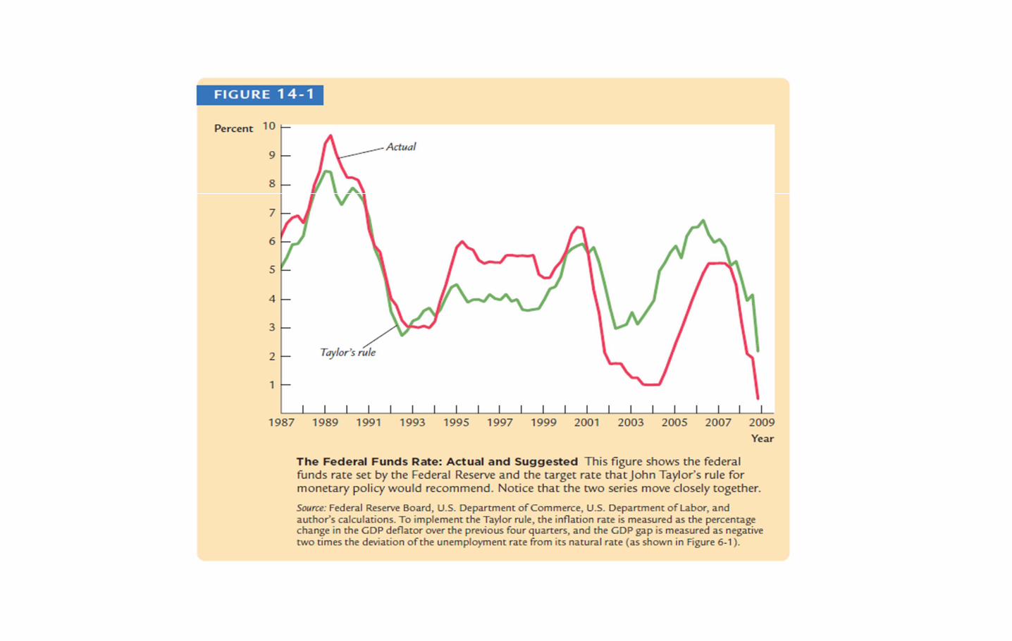
Nominal Federal Funds Rate = Inflation + 2.0 +
0.5 (Inflation − 2.0) + 0.5 (GDP gap).
GDP gap = the percentage by which real GDP deviates from an estimate of
its natural level.
the GDP gap is positive if GDP rises above its natural level and vice versa
According to the Taylor rule, the real federal funds rate—the nominal rate
minus inflation—responds to inflation and the GDP gap.

the Taylor rule for monetary policy also resembles actual Fed behavior in recent years.
Figure 14-1 Notice how the two series tend to move together. To some degree, it may be the rule that the Federal Reserve governors have been subconsciously following.

14.2 SOLVING THE MODEL
Output (�� )and the real interest rate ( �� )are at their natural values (�� , ρ)
inflation (π� )and expected inflation ((������ ) are at the target rate of inflation (π� *)
the nominal interest rate ( �� )equals the natural rate of interest(ρ) plus target inflation (π� *)
THE LONG RUN EQUILIBRIUM• The long-run equilibrium represents the normal state around which the economy
fluctuates.• occurs when there are no shocks (∈�= ��=0) • inflation has stabilized (��= ����).• Straightforward algebra applied to the above five equations can be used to verify
these long-run values:

The long-run equilibrium of this model reflects two related principles:1. the classical dichotomy : is the separation
of real from nominal variables 2. monetary neutrality : the property
according to which monetary policy does not influence real variables.
(π� *)
(π� ) ((������ ) ( �� )
variables—output (��) and the real interest rate (��)—do not depend on monetary policy.
In these ways, the long-run equilibrium of the dynamic AD–AS modelmirrors the classical models we examined in Chapters 3 to 8.

Kurva Dynamic Aggregate Supply
Kemiringan DAS ke atas: output tinggi berhubungan dengan inflasi tinggi.
Kemiringan DAS ke atas: output tinggi berhubungan dengan inflasi tinggi.
Y
π
DASt
1 ( ) t t t t tY Y
tY
t

Y
π
DASt
1 ( ) t t t t tY Y
tY
t
Any increase (decrease) in the previous period’s inflation or in the current period’s inflation shock shifts the DAS curve up (down) by the same amount
Any increase (decrease) in the previous period’s inflation or in the current period’s inflation shock shifts the DAS curve up (down) by the same amount
Kenaikan/ penurunan GDP menggeser kurva DAS ke kanan/ kiri dengan jumlah yang sama.
Kenaikan/ penurunan GDP menggeser kurva DAS ke kanan/ kiri dengan jumlah yang sama.
Kenaikan/ penurunan inflasi dari periode sebelumnya atau inflation shock periode saat ini menggeser kurva DAS naik atau turun dengan jumlah yang sama
Kenaikan/ penurunan inflasi dari periode sebelumnya atau inflation shock periode saat ini menggeser kurva DAS naik atau turun dengan jumlah yang sama
Pergeseran kurva DAS

Dynamic Aggregate Supply
ttttt
ttttt
ttttt
ttttt
YY
YY
YY
YY
1
1
1
1
1
1

Kurva Dynamic Aggregate Demand
( )t t t tY Y r
1( ) t t t t t tY Y i E
Rumus FisherRumus Fisher
1 tttt Eir
( ) t t t t tY Y i
adaptive expectations
adaptive expectations
tttE 1
Rumus Permintaan

( ) t t t t tY Y i
*[ ( ) ( ) ] t t t t t Y t t t tY Y Y Y
Kaidah kebijakan moneter
Kaidah kebijakan moneter
*[ ( ) ( )] t t t t Y t t tY Y Y Y
ttYtttt YYi *
Pusing mas & mbak? Sama...
Kurva Dynamic Aggregate Demand

Dynamic Aggregate Demand
*[ ( ) ( )] t t t t Y t t tY Y Y Y
t
Y
tt
Y
tt
ttttYtY
ttYttttYt
ttYtYtttt
YY
YY
YYYY
YYYY
1
1)(
1
)()1()1(
)(
)(
*
*
*
*
Alhamdulillah, Inilah Rumus DAD*
*Mari kita berdoa semoga ujiannya open book

Kurva Dynamic Aggregate Demand
Kemiringan kurva DAD ke bawah:Ketika inflasi naik, bank sentral akan menaikkan tingkat bunga riil, sehingga mengurangi permintaan barang dan jasa
Kemiringan kurva DAD ke bawah:Ketika inflasi naik, bank sentral akan menaikkan tingkat bunga riil, sehingga mengurangi permintaan barang dan jasa
Y
π
DADt
t
Y
tt
Y
tt YY
1
1)(
1*

Y
π
DADtB
*t
Ketika target inflasi bank sentral naik atau turun, maka kurva DAD juga akan bergeser naik atau turun dengan jumlah yang sama.
DADtA
Kurva Dynamic Aggregate Demand
t
Y
tt
Y
tt YY
1
1)(
1*
t
Y
tt YY
1
1

Y
π
DADtB
*t
Ketika tingkat output alami mengalami kenaikan/ penurunan, maka kurva DAD akan bergeser ke kanan/ kiri dengan jumlah yang sama.
DADtA
t
Y
tt
Y
tt YY
1
1)(
1*
Kurva Dynamic Aggregate Demand
t
Y
tt YY
1
1

Yt
Keseimbangan jangka pendek
Dalam setiap periode, pertemuan antara DAD dan DAS menentukan nilai inflasi dan output pada keseimbangan jangka pendek
Dalam setiap periode, pertemuan antara DAD dan DAS menentukan nilai inflasi dan output pada keseimbangan jangka pendek
πt
Yt
Y
π
DADt
DASt
A
Dalam kurva di samping, output sebesar A berada di bawah tingkat output natural, yang berarti perekonomian sedang mengalami resesi.
Dalam kurva di samping, output sebesar A berada di bawah tingkat output natural, yang berarti perekonomian sedang mengalami resesi.

Periode t: keseimbangan awal pada A
Periode t: keseimbangan awal pada A
Periode t + 1: Pertumbuhan jangka panjang meningkatkan tingkat output natural
Periode t + 1: Pertumbuhan jangka panjang meningkatkan tingkat output natural
DAS bergeser ke kanan sejumlah peningkatan output natural (GDP natural)
DAS bergeser ke kanan sejumlah peningkatan output natural (GDP natural)
DAD juga bereser ke kanan sejumlah peningkatan output natural (GDP natural)
DAD juga bereser ke kanan sejumlah peningkatan output natural (GDP natural)
Keseimbangan baru pada B. Pendapatan bertambah tapi inflasi tetap.Keseimbangan baru pada B. Pendapatan bertambah tapi inflasi tetap.
Yt
A
Yt
DAStDASt +1
DADt +1
Yt +1
B
Y
π
DADt
πt + 1
πt
=
Yt +1
Pertumbuhan Jangka Panjang

Shock pada penawaran aggregate Periode t–1: keseimbangn awal di APeriode t–1: keseimbangn awal di A
Periode t: Supply shock (νt
> 0) menggeser DAS ke atas; inflasi naik, bank sentral merespon dengan menaikkan tingkat bunga riil, akibatnya output turun
Periode t: Supply shock (νt
> 0) menggeser DAS ke atas; inflasi naik, bank sentral merespon dengan menaikkan tingkat bunga riil, akibatnya output turun
Periode t + 1: Supply shock sudah reda (νt+1 = 0) tapi DAS tidak kembali ke posisi awal karena ekspektasi inflasi yang tinggi
Periode t + 1: Supply shock sudah reda (νt+1 = 0) tapi DAS tidak kembali ke posisi awal karena ekspektasi inflasi yang tinggi
Periode t + 2: Ketika inflasi turun, ekspektasi inflasi juga turun, DAS bergeser ke bawah, output naik.
Periode t + 2: Ketika inflasi turun, ekspektasi inflasi juga turun, DAS bergeser ke bawah, output naik.
A
Yt
Bπt
DASt
DASt +1
C
πt – 1
Yt –1
Y
π
DASt -1
Y
DAD
DASt +2
D
Yt + 2
πt + 2
Proses ini berlanjut sampai outputkembali ke tingkat natural.Keseimbangan jangka panjangkembali ke A.

Respon dinamis terhadap supply shock
tY
t
Satu perode supply shock
memengaruhi
output untuk
beberapa periode.
Satu perode supply shock
memengaruhi
output untuk
beberapa periode.

t
tKarena ekspektasi
inflasi susah
menyesuaikan,
inflasi aktual tetap tinggi
dalam
beberapa
periode
Karena ekspektasi
inflasi susah
menyesuaikan,
inflasi aktual tetap tinggi
dalam
beberapa
periode
Respon dinamis terhadap supply shock

tr
t
Tingkat bunga riil
membutuhkan
beberapa
periode untuk kembali ke
tingkat natural
Tingkat bunga riil
membutuhkan
beberapa
periode untuk kembali ke
tingkat natural
Respon dinamis terhadap supply shock

ti
tTingkat bunga nominal
ditetapkan
bergantung
pada inflasi dan tingkat
bunga riil
Tingkat bunga nominal
ditetapkan
bergantung
pada inflasi dan tingkat
bunga riil
Respon dinamis terhadap supply shock

Shock pada permintaan aggregate Periode t – 1: keseimbangan awal di APeriode t – 1: keseimbangan awal di A
Periode t: Demand shock (ε > 0) menggeser DAD ke kanan; output dan inflasi naik.
Periode t: Demand shock (ε > 0) menggeser DAD ke kanan; output dan inflasi naik.
Periode t + 1: Inflasi tinggi di tmemicu ekspektasi inflasi juga tinggi di t + 1, shg menggeser DAS naik. Inflasi aktual naik dan output turun.
Periode t + 1: Inflasi tinggi di tmemicu ekspektasi inflasi juga tinggi di t + 1, shg menggeser DAS naik. Inflasi aktual naik dan output turun.
Periode t + 2 ke t + 4:Inflasi tinggi pada periode sebelumnya masih memicu ekspektasi inflasi naik lebih tinggi, shg kurva DAS masih naik. Inflasi semakin naik, dan output semakin turun.
Periode t + 2 ke t + 4:Inflasi tinggi pada periode sebelumnya masih memicu ekspektasi inflasi naik lebih tinggi, shg kurva DAS masih naik. Inflasi semakin naik, dan output semakin turun.
Periode t + 5: DAS masih tinggi akibat inflasi tinggi pada periode sebelumnya, tapi demand berakhir dan DAD kembali ke posisi semula. Keseimbangan di G.
Periode t + 5: DAS masih tinggi akibat inflasi tinggi pada periode sebelumnya, tapi demand berakhir dan DAD kembali ke posisi semula. Keseimbangan di G.
DADt -1, t+5
πt – 1 DADt ,t+1,…,t+4A
Y
Yt –1
Y
π
DASt -1,t
DASt +5
DASt + 1
C
DASt +2
D
DASt +3
E
DASt +4
F
Yt
Bπt
Yt + 5
Gπt + 5
Periode t + 6 dan selanjutnya:DAS scr bertahap turun seiring inflasi dan ekspektasi inflasi juga turun. Perekonomian membaik dan kembali ke keseimbangan jangka panjang di A.
Periode t + 6 dan selanjutnya:DAS scr bertahap turun seiring inflasi dan ekspektasi inflasi juga turun. Perekonomian membaik dan kembali ke keseimbangan jangka panjang di A.

Respon dinamis pada demand shock
tY
t
Demand shock memicu
naiknya output
dalam lima
periode. Ketika shock
berakhir,,
output turun di
bawah tingkat
natural, dan
membaik
kembali secara
bertahap.
Demand shock memicu
naiknya output
dalam lima
periode. Ketika shock
berakhir,,
output turun di
bawah tingkat
natural, dan
membaik
kembali secara
bertahap.

t
t
Demand shock menyebabkan
inflasi naik.
Ketika shock
berakhir, inflasi secara
bertahap turun
ke posisi awal.
Demand shock menyebabkan
inflasi naik.
Ketika shock
berakhir, inflasi secara
bertahap turun
ke posisi awal.
Respon dinamis pada demand shock
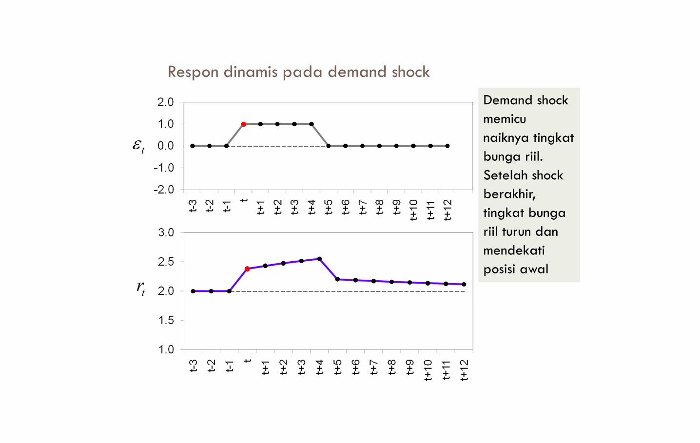
tr
t
Demand shock memicu
naiknya tingkat
bunga riil.
Setelah shock berakhir,
tingkat bunga
riil turun dan
mendekati posisi awal
Demand shock memicu
naiknya tingkat
bunga riil.
Setelah shock berakhir,
tingkat bunga
riil turun dan
mendekati posisi awal
Respon dinamis pada demand shock

ti
t
Tingkat bunga nominal
bergantung
pada inflasi
dan tingkat bunga riil
Tingkat bunga nominal
bergantung
pada inflasi
dan tingkat bunga riil
Respon dinamis pada demand shock

A shift in monetary policyPeriod t – 1: target inflation rate π* = 2%, initial equilibrium at A
Period t – 1: target inflation rate π* = 2%, initial equilibrium at A
πt – 1 = 2%
Yt –1
Period t: Central bank lowers target to π* = 1%, raises real interest rate, shifts DAD leftward. Output and inflation fall.
Period t: Central bank lowers target to π* = 1%, raises real interest rate, shifts DAD leftward. Output and inflation fall.Period t + 1: The fall in πt reduced inflation expectations for t + 1, shifting DAS downward. Output rises, inflation falls.
Period t + 1: The fall in πt reduced inflation expectations for t + 1, shifting DAS downward. Output rises, inflation falls.
Y
πDASt -1, t
Y
DADt – 1
A
DADt, t + 1,…
DASfinal
Yt
πtB
DASt +1
C
Subsequent periods:This process continues until output returns to its natural rate and inflation reaches its new target.
Subsequent periods:This process continues until output returns to its natural rate and inflation reaches its new target.
Zπfinal = 1%
,
Yfinal

The dynamic response to a reduction in target inflation
tY
*t
Reducing the target
inflation rate
causes output
to fall below its natural
level for a
while.
Output
recovers
gradually.
Reducing the target
inflation rate
causes output
to fall below its natural
level for a
while.
Output
recovers
gradually.

The dynamic response to a reduction in target inflation
t
*t Because
expectations
adjust slowly,
it takes many
periods for inflation to
reach the new
target.
Because expectations
adjust slowly,
it takes many
periods for inflation to
reach the new
target.

The dynamic response to a reduction in target inflation
tr
*t
To reduce inflation,
the central
bank raises
the real interest rate
to reduce
aggregate
demand.The real
interest rate
gradually
returns to its
natural rate.
To reduce inflation,
the central
bank raises
the real interest rate
to reduce
aggregate
demand.The real
interest rate
gradually
returns to its
natural rate.

The dynamic response to a reduction in target inflation
ti
*t
The initial increase in
the real
interest rate
raises the nominal
interest rate.
As the
inflation and real interest
rates fall,
the nominal
rate falls.
The initial increase in
the real
interest rate
raises the nominal
interest rate.
As the
inflation and real interest
rates fall,
the nominal
rate falls.

APPLICATION:
Output variability vs. inflation variability
A supply shock reduces output (bad) and raises inflation (also bad).
The central bank faces a tradeoff between these “bads” – it can reduce the effect on output, but only by tolerating an increase in the effect on inflation….

APPLICATION:
Output variability vs. inflation variability
CASE 1: θπ is large, θY is small
Y
π
DADt – 1, t
DASt
DASt – 1
Yt –1
πt –1
Yt
πt
A supply shock shifts DAS up.A supply shock shifts DAS up.
In this case, a small change in inflation has a large effect on output, so DAD is relatively flat.
In this case, a small change in inflation has a large effect on output, so DAD is relatively flat.
The shock has a large effect on output, but a small effect on inflation.
The shock has a large effect on output, but a small effect on inflation.

APPLICATION:
Output variability vs. inflation variability
CASE 2: θπ is small, θY is large
Y
π
DADt – 1, t
DASt
DASt – 1
Yt –1
πt –1
Yt
πt
In this case, a large change in inflation has only a small effect on output, so DAD is relatively steep.
In this case, a large change in inflation has only a small effect on output, so DAD is relatively steep.
Now, the shock has only a small effect on output, but a big effect on inflation.
Now, the shock has only a small effect on output, but a big effect on inflation.

APPLICATION:
The Taylor Principle
The Taylor Principle (named after economist John Taylor): The proposition that a central bank should respond to an increase in inflation with an even greater increase in the nominal interest rate (so that the real
interest rate rises). I.e., central bank should set θπ > 0.
Otherwise, DAD will slope upward, economy may be unstable, and inflation may spiral out of control.

APPLICATION:
The Taylor Principle
If θπ > 0:
• When inflation rises, the central bank increases the nominal interest rate even more, which increases the real interest rate and reduces the demand for goods and services.
• DAD has a negative slope.
* 1( )
1 1
t t t t t
Y Y
Y Y
(DAD)
*( ) ( ) t t t t Y t ti Y Y (MP rule)

APPLICATION:
The Taylor Principle
If θπ < 0:
• When inflation rises, the central bank increases the nominal interest rate by a smaller amount. The real interest rate falls, which increases the demand for goods and services.
• DAD has a positive slope.
* 1( )
1 1
t t t t t
Y Y
Y Y
(DAD)
*( ) ( ) t t t t Y t ti Y Y (MP rule)
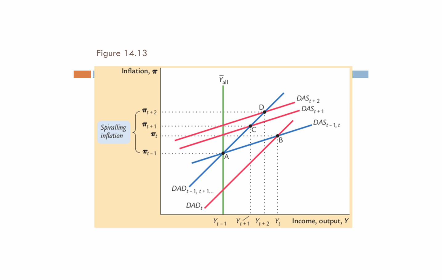
Figure 14.13


