Page 1
A Dynamic Parameter Identification Method for MigratingControl Strategies Between Heterogeneous Wheeled Mobile
Robots
by
Jeffrey Laut
A Thesis
Submitted to the Faculty
of the
WORCESTER POLYTECHNIC INSTITUTE
In partial fulfillment of the requirements for the
Degree of Master of Science
in
Mechanical Engineering
by
May 2011
APPROVED:
Professor Michael A. Demetriou, Thesis Advisor
Professor Stephen S. Nestinger, Thesis Advisor
Professor Gregory S. Fischer, Graduate Committee Member
Professor Nikolaos A. Gatsonis, Graduate Committee Representative
Page 2
Abstract
Recent works on the control of wheeled mobile robots have shifted from the use
of the kinematic model to the use of the dynamic model. Since theoretical results
typically treat the inputs to the dynamic model as torques, few experimental re-
sults have been provided, as torque is typically not the input to most commercially
available robots. Few papers have implemented controllers based on the dynamic
model, and those that have did not address the issue of identifying the parameters
of the dynamic model.
This work focuses on a method for identifying the parameters of the dynamic model
of a wheeled mobile robot. The method is shown to be both effective and easy to
implement, and requires no prior knowledge of what the parameters may be. Exper-
imental results on two mobile robots of different scale demonstrate its effectiveness.
The estimates of the parameters created by the proposed method are then used in
an adaptive controller to verify their accuracy. For future work, this method should
be completed autonomously in a two-part manner, onboard the mobile robot. First,
the robot should perform the method proposed here to generate an initial parameter
estimate, and then use adaptive control to update the estimates.
Page 3
Acknowledgements
I would like to show my gratitude to my advisors, Prof. Demetriou and Prof.
Nestinger, who have both given me excellent guidance and support.
Thanks to the Mechanical Engineering department for the supporting my education
through a teaching assistantship. Working with Professors Furlong, Gatsonis, and
Sullivan was a rewarding experience.
I am grateful to Prof. Fischer, who provided me with much appreciated feedback
regarding the content and structure of my thesis.
Thanks to Yue Wang for the insightful conversations, and thanks to the rest of the
friends I have made at WPI, including Jeff Court, Shalin Ye, Yao Wang, Mahdi
Agheli, and Brendan Chenelle.
A special thanks to my parents. If it wasn’t for them, I probably wouldn’t have
even gone to college!
i
Page 4
Contents
1 Introduction 1
2 Modeling Differential-Drive Wheeled Mobile Robots 4
2.1 Kinematics of Wheeled Mobile Robots. . . . . . . . . . . . . . . . . . 4
2.2 Parameterized Dynamic Model . . . . . . . . . . . . . . . . . . . . . 8
3 Control Based on the Dynamic Model 15
3.1 Odometry . . . . . . . . . . . . . . . . . . . . . . . . . . . . . . . . . 16
3.2 Inverse Dynamic Control . . . . . . . . . . . . . . . . . . . . . . . . . 17
3.3 Adaptation of Dynamic Parameters . . . . . . . . . . . . . . . . . . . 21
4 Parameter Estimation 23
4.1 Proposed method . . . . . . . . . . . . . . . . . . . . . . . . . . . . . 23
4.2 Simulation Results . . . . . . . . . . . . . . . . . . . . . . . . . . . . 29
4.3 Experimental Setup . . . . . . . . . . . . . . . . . . . . . . . . . . . . 41
4.4 Experimental Results . . . . . . . . . . . . . . . . . . . . . . . . . . . 44
4.4.1 Khepera III . . . . . . . . . . . . . . . . . . . . . . . . . . . . 46
4.4.2 Pioneer 3-DX . . . . . . . . . . . . . . . . . . . . . . . . . . . 59
5 Conclusions and Future Work 69
5.1 Conclusions . . . . . . . . . . . . . . . . . . . . . . . . . . . . . . . . 69
ii
Page 5
5.2 Future Work . . . . . . . . . . . . . . . . . . . . . . . . . . . . . . . . 70
A Generating a Trajectory 71
A.1 Figure Eight . . . . . . . . . . . . . . . . . . . . . . . . . . . . . . . . 71
A.2 Figure Eight with Dither . . . . . . . . . . . . . . . . . . . . . . . . . 73
A.3 Alterative Parameterized Dynamic Model . . . . . . . . . . . . . . . . 76
B Installing and Using the Khepera III Toolbox 80
B.1 Installing the toolbox . . . . . . . . . . . . . . . . . . . . . . . . . . . 80
B.2 Writing a program . . . . . . . . . . . . . . . . . . . . . . . . . . . . 81
iii
Page 6
List of Figures
2.1 Coordinates for a disk on plane [9] . . . . . . . . . . . . . . . . . . . 5
2.2 Coordinates for unicycle on plane [9] . . . . . . . . . . . . . . . . . . 5
2.3 Differential-drive mobile robot . . . . . . . . . . . . . . . . . . . . . . 6
2.4 Terms of dynamic model of differential-drive mobile robot . . . . . . 8
4.1 Legend for parameter evolution plots . . . . . . . . . . . . . . . . . . 30
4.2 Perfect initial estimates . . . . . . . . . . . . . . . . . . . . . . . . . 30
4.3 Effect of control gain on parameter convergence . . . . . . . . . . . . 31
4.4 Angular velocity and θ6 . . . . . . . . . . . . . . . . . . . . . . . . . . 32
4.5 Parameter evolution for figure-eight trajectory . . . . . . . . . . . . . 33
4.6 Parameter evolution for figure-eight trajectory with dither . . . . . . 34
4.7 Evolution of θ5 . . . . . . . . . . . . . . . . . . . . . . . . . . . . . . 35
4.8 Parameter evolution . . . . . . . . . . . . . . . . . . . . . . . . . . . 36
4.9 Parameter evolution . . . . . . . . . . . . . . . . . . . . . . . . . . . 37
4.10 Regression . . . . . . . . . . . . . . . . . . . . . . . . . . . . . . . . 39
4.11 Khepera III and Pioneer 3-DX mobile robots . . . . . . . . . . . . . . 42
4.12 Khepera III trajectory and error, with adaptation, poor initial esti-
mates . . . . . . . . . . . . . . . . . . . . . . . . . . . . . . . . . . . 47
4.13 Velocity data . . . . . . . . . . . . . . . . . . . . . . . . . . . . . . . 48
4.14 Acceleration data . . . . . . . . . . . . . . . . . . . . . . . . . . . . . 49
iv
Page 7
4.15 Plots of linear regression . . . . . . . . . . . . . . . . . . . . . . . . . 50
4.16 Khepera III trajectory and error, no adaptation . . . . . . . . . . . . 51
4.17 Khepera III trajectory and error, with adaptation . . . . . . . . . . . 52
4.18 Comparison of figures 4.16 and 4.17 . . . . . . . . . . . . . . . . . . 53
4.19 Khepera III trajectory and error with heavy payload, no adaptation 54
4.20 Khepera III trajectory and error with heavy payload, with adapta-
tion. . . . . . . . . . . . . . . . . . . . . . . . . . . . . . . . . . . . . 55
4.21 Khepera III trajectory and error with light payload, no adaptation. . 56
4.22 Khepera III trajectory and error with light payload, with adaptation. 57
4.23 Comparison of Figures 4.21 and 4.22 . . . . . . . . . . . . . . . . . . 58
4.24 Pioneer 3-DX trajectory and error, poor initial estimates, with adap-
tation. . . . . . . . . . . . . . . . . . . . . . . . . . . . . . . . . . . 60
4.25 Velocity data . . . . . . . . . . . . . . . . . . . . . . . . . . . . . . . 61
4.26 Acceleration data . . . . . . . . . . . . . . . . . . . . . . . . . . . . . 62
4.27 Plots of linear regression. . . . . . . . . . . . . . . . . . . . . . . . . 63
4.28 Pioneer 3-DX trajectory and error, adapting all parameters except θ4
and θ6 . . . . . . . . . . . . . . . . . . . . . . . . . . . . . . . . . . . 65
4.29 Pioneer 3-DX trajectory and error, heavy payload, no adaptation . . 66
4.30 Pioneer 3-DX trajectory and error, heavy payload, with adaptation . 68
v
Page 8
List of Tables
2.1 List of terms of dynamic model . . . . . . . . . . . . . . . . . . . . . 9
4.1 Parameter final and initial values . . . . . . . . . . . . . . . . . . . . 33
4.2 Parameter final and initial values . . . . . . . . . . . . . . . . . . . . 34
4.3 Khepera III steady state velocity values . . . . . . . . . . . . . . . . 45
4.4 Pioneer 3-DX steady state velocity values . . . . . . . . . . . . . . . 45
vi
Page 9
Chapter 1
Introduction
Wheeled mobile robots are becoming more popular for performing tasks that are
too dangerous or tedious for humans, and with the increase in available technology,
it is becoming more cost-effective to replace a worker with a mobile robot. Typical
environments for wheeled mobile robots include warehouses, factories, military ap-
plications, and planetary exploration. In situations where the robot must maneuver
with precision, a feedback controller for robot motion is necessary.
Regarding the control of wheeled mobile robots, early papers typically focused on
using only the kinematics. It was shown through simulations in [1] that for high
speed and high load situations, the dynamics of the robot should be considered for
better performance in trajectory tracking. Most of the research regarding control
based on the dynamic model has shown only simulation results.
For instance, [2] was the first paper to consider control using the dynamic model
with unknown dynamics, and provided torques as inputs to the model, and showed
simulation results. [3] provided a controller based on the dynamic model that took
inputs from a kinematic controller, and altered them to compensate for the dynam-
1
Page 10
ics of a robot. In [4], a combined kinematic and dynamic control law was presented.
Their model also assumed torques as input, and provided only simulation results. [5]
created a simplified dynamic model, and analyzed the influence of the uncertainties.
They too treated the inputs as torques, and provided only simulation results.
Most of the controllers based on the dynamic model considered torques as the in-
puts, however most commercially available robots do not take torques as inputs. In
an effort to design a more practical controller, [6] developed a controller that used
voltages as inputs to the dynamic model, but only provided simulation results. [7]
created a controller that gave current as input to the dynamic model, and provided
experimental results on a custom robot for adaptive steering and adaptive cruise
control. More recently [8] provided a dynamic model based on the parameterization
from [5], which provided reference velocities as inputs. This is the most practical
situation, as most commercially available robots take reference velocities as inputs.
A field of research that seems to have remained mostly untouched, likely due to only
the recent use of the dynamic model in control of mobile robots in experiments, is
the identification of the parameters of wheeled mobile robots. This work addresses
the problem of creating an initial estimate for the parameters of a wheeled mobile
robot, and provides experimental results showing both its need and effectiveness.
This thesis is organized as follows; In Chapter 2, first the kinematics of a differential
drive mobile robot are reviewed. The dynamic model of a mobile robot which takes
velocities as inputs, and includes actuator dynamics is then derived, followed by an
overview of odometry as a feedback mechanism. Controlling the robot using the
dynamic model is discussed in Chapter 3, assuming that the constants the represent
2
Page 11
physical parameters of the robot are perfectly known. To overcome this assumption,
an adaptive controller which updates the estimates of the unknown parameters of
the robot is shown. To implement the adaptive controller on physical robots, a
reasonable initial estimate of the parameters must first be generated. The main
contribution is located in Chapter 4, which covers how to create an appropriate
initial estimate. Simulation results are provided, and experimental results for two
different robots are shown at the end of the chapter.
In the future, we would like to have a two-part scheme that first executes the pro-
posed method to generate initial parameter estimates, and then uses adaptive control
to further tune the parameters. This scheme should be completed entirely on-board
the robot. Furthermore, we would like the scheme to be easily transferable between
heterogeneous mobile robots.
3
Page 12
Chapter 2
Modeling Differential-Drive
Wheeled Mobile Robots
2.1 Kinematics of Wheeled Mobile Robots.
The pose a mobile robot is defined by three coordinates represented by the vector
ξ,
ξ =
x
y
φ
(2.1)
The set of reachable poses defined by C encompasses the plane that the robot is
maneuvering about. The motion of ξ, however, is subject to a nonholonomic con-
straint. This constraint means that the kinematic model of the robot is not capable
of producing instantaneous motion in any direction. To illustrate this, we observe
the kinematic constraint of a unicycle model on a plane. Since the unicycle cannot
move in the direction perpendicular to the plane containing the wheel, its motion is
constrained by x sinφ = y cosφ. Although this constraint restricts the robot from
4
Page 13
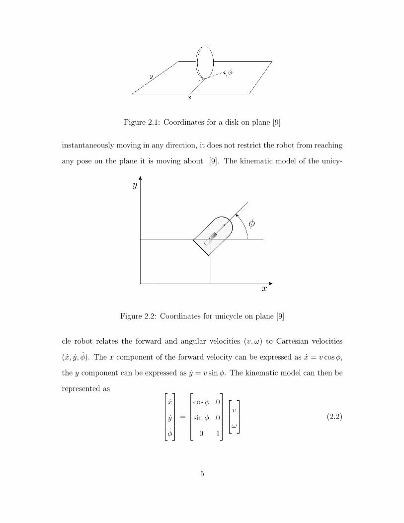
Figure 2.1: Coordinates for a disk on plane [9]
instantaneously moving in any direction, it does not restrict the robot from reaching
any pose on the plane it is moving about [9]. The kinematic model of the unicy-
Figure 2.2: Coordinates for unicycle on plane [9]
cle robot relates the forward and angular velocities (v, ω) to Cartesian velocities
(x, y, φ). The x component of the forward velocity can be expressed as x = v cosφ,
the y component can be expressed as y = v sin φ. The kinematic model can then be
represented as
x
y
φ
=
cosφ 0
sinφ 0
0 1
v
ω
(2.2)
5
Page 14
or
ξ = S(ξ)v (2.3)
where v =
[
v ω
]⊤
and S(ξ) is the transformation matrix that relates v and ξ.
A differential-drive robot has the same kinematic constraint and kinematic model
as the unicycle model. The only additional work needed is to relate the forward
and angular velocities of the unicycle with the individual wheel velocities for the
differential drive robot.
v =r(ωr + ωl)
2, ω =
r(ωr − ωl)
d(2.4)
where ωr and ωl are the right and left wheel rotational velocities, r is the radius of
r
d
v
ω
Figure 2.3: Differential-drive mobile robot
the wheels, and d is the distance between the wheels (Figure 2.3).
From the two equations above, the individual wheel velocities can be found as a
6
Page 15
function of v and ω,
ωr =2v + dω
2r, ωl =
2v − dω
2r(2.5)
Typically, throughout an analysis of a control scheme for a differential drive robot,
the unicycle model is used. In this case, the inputs to the kinematic model are still v
and ω, and the wheel velocities are only calculated when the controller is physically
implemented.
This section provided information on transforming between a robot’s forward and
angular velocities to Cartesian velocities. As stated previously, early works focused
on controlling a mobile robot using only the kinematic model. This assumes that
any velocity v or ω given to the robot is instantaneously achieved, and does not
account for dynamic effects of the robot. To accurately model the motion of a
wheeled mobile robot, the dynamics should be accounted for [1], as a mobile robot
in practice cannot achieve instantaneous acceleration. The inputs to the dynamic
model generate the forward and angular velocities of the mobile robot, which can
then be used with the kinematic model to provide Cartesian velocities. The next
section derives a parameterized dynamic model, where the parameters are physical
constants of the model, and vary from robot to robot.
7
Page 16
2.2 Parameterized Dynamic Model
A parameterized dynamic model of a differential-drive mobile robot, including actu-
ator dynamics, was presented in [5]. This model treated the inputs to the motors as
torques. In [8], the same parameterized model was used, with the alteration of using
reference velocities as the motor inputs. Their model considered a proportional-
derivative controller on the forward and angular velocity inputs. Another common
configuration is to have proportional-derivative control on the individual wheel ve-
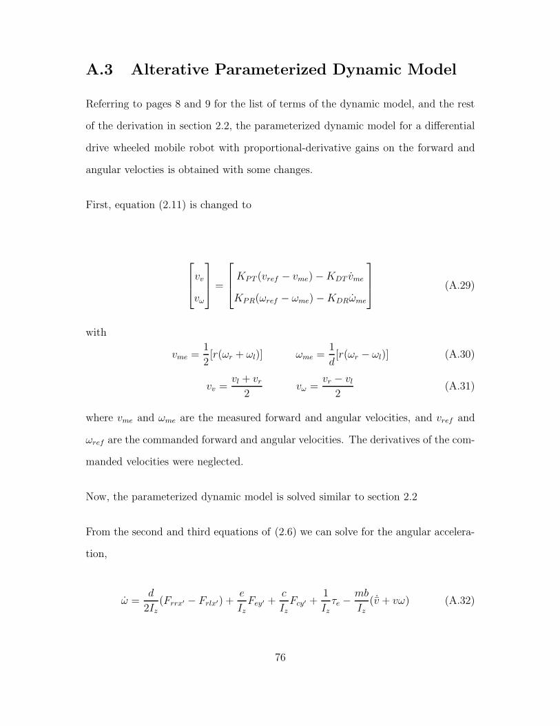
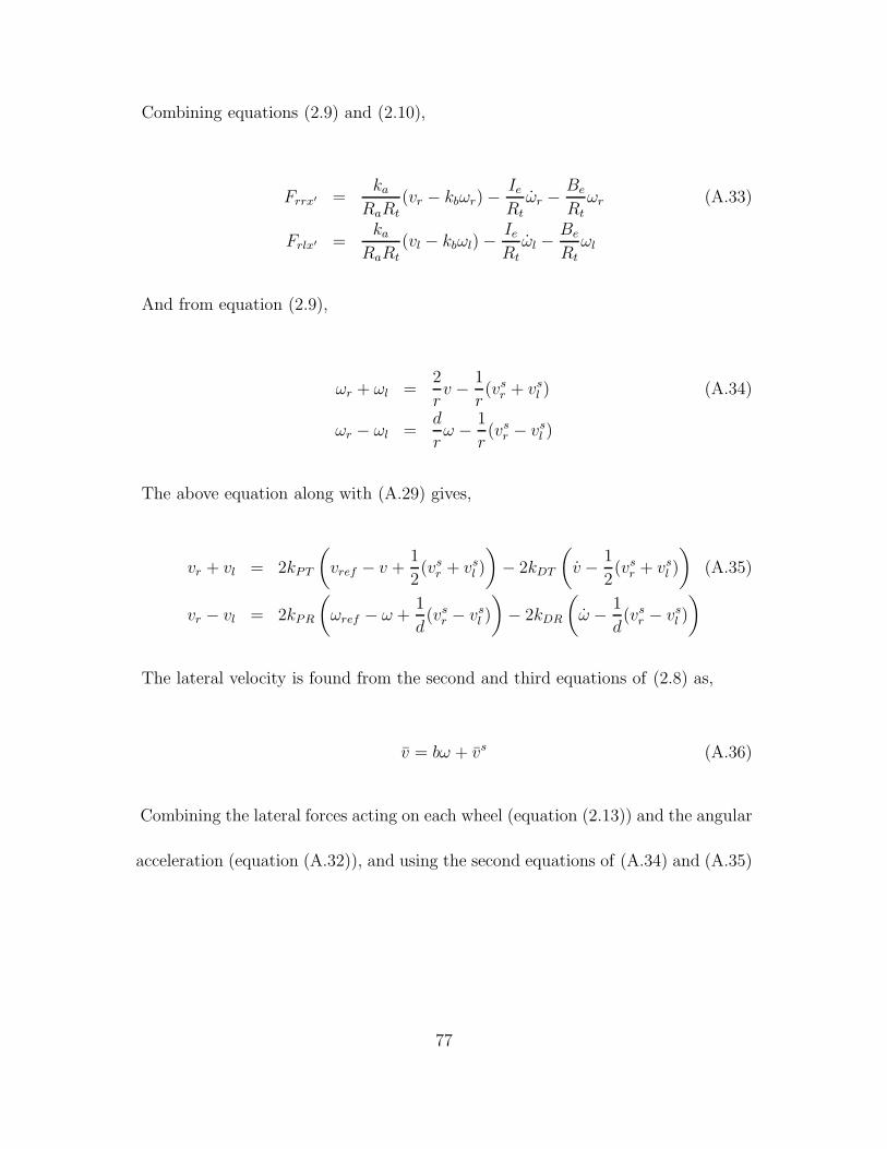
locities. In this section, the parameterized dynamic model for a mobile robot with
proportional-derivative control on the individual wheel velocities is derived. The
parameterized dynamic model for a mobile robot with a proportional-derivative
controller on the forward and angular velocities is shown in Appendix A.3.
Figure 2.4: Terms of dynamic model of differential-drive mobile robot
8
Page 17
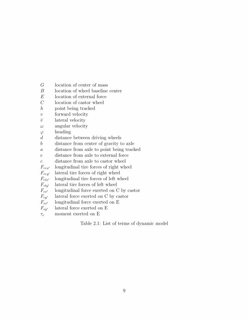
G location of center of massB location of wheel baseline centerE location of external forceC location of castor wheelh point being trackedv forward velocityv lateral velocityω angular velocityϕ headingd distance between driving wheelsb distance from center of gravity to axlea distance from axle to point being trackede distance from axle to external forcec distance from axle to castor wheelFrrx′ longitudinal tire forces of right wheelFrry′ lateral tire forces of right wheelFrlx′ longitudinal tire forces of left wheelFrly′ lateral tire forces of left wheelFcx′ longitudinal force exerted on C by castorFcy′ lateral force exerted on C by castorFex′ longitudinal force exerted on EFey′ lateral force exerted on Eτe moment exerted on E
Table 2.1: List of terms of dynamic model
9
Page 18
First, we find the robot force and moment equations about local coordinate frame:
ΣFx′ = m(v − vω) = Frlx′ + Frrx′ + Fex′ + Fcx′
ΣFy′ = m( ˙v − vω) = Frly′ + Frry′ + Fey′ + Fcy′ (2.6)
ΣMz′ = Izω =d
2(Frrx′ − Frlx′)− b(Frly′ + Frry′) · · ·
+(e− b)Fey′ + (c− b)Fcy′ + τe,
where m is the mass of the robot and Iz is the robot moment of inertia about the
local z′ axis.
The kinematics of the point being tracked, h, are;
x = v cosψ − v sinψ − (a− b)ω sinψ (2.7)
y = v sinψ − v cosψ + (a− b)ω cosψ,
with
v =1
2[r(ωr + ωl) + (vsr + vsl )]
ω =1
d[r(ωr − ωl) + (vsr − vsl )] (2.8)
v =b
d[r(ωr − ωl) + (vsr + vsl )] + vs,
where v is the forward velocity, ω is the angular velocity, v is the lateral velocity, vr
and vl are the left and right linear velocities of each wheel, and any velocity with
an s superscript is a velocity due to wheel slippage.
10
Page 19
The dynamic model of the drive motors are obtained by neglecting the voltage on
the inductance as:
τr = ka(vr − kbωr)/Ra τl = ka(vl − kbωl)/Ra, (2.9)
where vr and vl are the input voltages applied to the right and left motors, kb is the
motor voltage constant multiplied by the gear ratio, Ra is the electrical resistance
constant, τr and τl are the right and left motor torques multiplied by the gear ratio,
and ka is the torque constant multiplied by the gear ratio.
The dynamics of the combined wheels and motors are:
Ieωr +Beωr = τr − Frrx′Rt (2.10)
Ieωl +Beωl = τl − Frlx′Rt,
where Ie is the moment of inertia and Be is the viscous friction coefficient of the
motor, gearbox, and wheel combination, and Rt is the radius of the tire.
The voltage applied to each motor is given by the output of the onboard motor
controller. This is a proportional-derivative controller, and the dynamics of the
motor input voltage are:
vl = kP (ωlref − ωl) + kDωl (2.11)
vr = kP (ωrref − ωr) + kDωr,
where ωlref and ωrref are the commanded left and right wheel velocities, and ωl and
11
Page 20
ωr are the actual wheel velocities. The derivatives of the commanded velocities were
neglected since the robot cannot be given a reference acceleration.
The above equations are now manipulated in order to arrive at the parameterized
dynamic model of the robot.
From the second and third equations of (2.6) we can solve for the angular accelera-
tion,
ω =d
2Iz(Frrx′ − Frlx′) +
e
IzFey′ +
c
IzFcy′ +
1
Izτe −
mb
Iz( ˙v + vω). (2.12)
Combining equations (2.9) and (2.10),
Frrx′ =ka
RaRt
(vr − kbωr)−IeRt
ωr −Be
Rt
ωr (2.13)
Frlx′ =ka
RaRt
(vl − kbωl)−IeRt
ωl −Be
Rt
ωl,
and from equation (2.9),
ωr + ωl =2
rv −
1
r(vsr + vsl ) (2.14)
ωr − ωl =d
rω −
1
r(vsr − vsl ).
The above equation along with (2.11) gives,
12
Page 21
vr + vl = kP (ωrref + ωlref )− kD(ωr + ωl)−2kPrv +
kPr(vsr + vsl ) (2.15)
vr − vl = kP (ωrref − ωlref )− kD(ωr − ωl)−kPd
rω +
kPr(vsr − vsl ).
From equation (2.8),
ωr + ωl =2v − (vsr + vsl )
r(2.16)
ωr − ωl =ωd− (vsr − vsl )
r.
Combining the lateral forces acting on each wheel (equation (2.13)) and the angular
acceleration (equation (2.12)), and using the second equations of (2.14) and (2.15)
as well as the above equation, and using the following parameterization,
θ1 =RaRtm+ 2kakD + 2IeRa
2kakP
θ2 =kakDd
2 + IeRad2 + 2RaRtr(mb
2 + Iz)
kakPd2
θ3 =RaRtrm
2kakP
θ4 =ka(kP + kb) + 2RaBe
2kakP
θ5 =2RaRtrmb
kakPd2
θ6 =RaRt(kP + kb) +RaBe
kakP
gives,
θ2ω = ωref − θ6ω +1
dθ6(v
sr − vsl ) +
kakD +RaIekakPd
(vsr − vsl ) +
2RaRtr
kakpd2(eFey′ + cFcy′ + τe)− θ5 ˙v
s − θ5vω. (2.17)
13
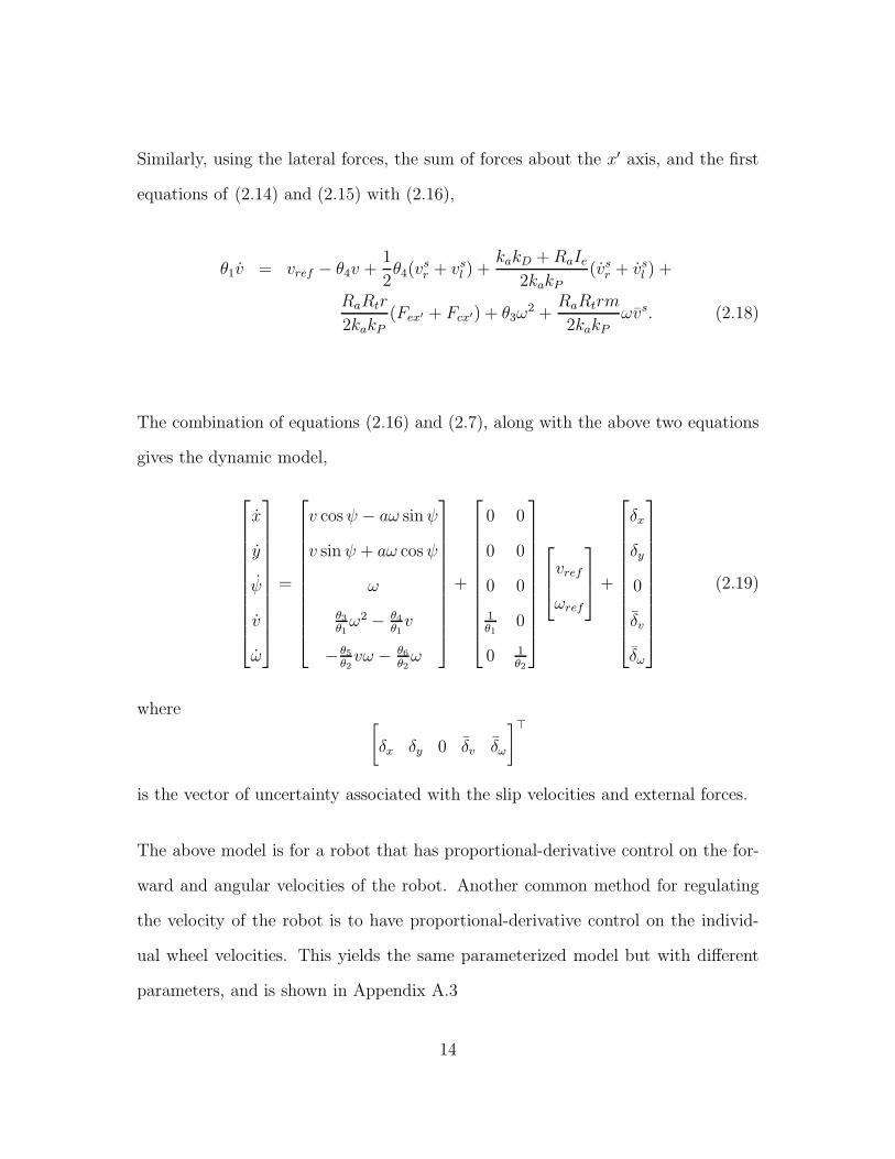
Page 22
Similarly, using the lateral forces, the sum of forces about the x′ axis, and the first
equations of (2.14) and (2.15) with (2.16),
θ1v = vref − θ4v +1
2θ4(v
sr + vsl ) +
kakD +RaIe2kakP
(vsr + vsl ) +
RaRtr
2kakP(Fex′ + Fcx′) + θ3ω
2 +RaRtrm
2kakPωvs. (2.18)
The combination of equations (2.16) and (2.7), along with the above two equations
gives the dynamic model,
x
y
ψ
v
ω
=
v cosψ − aω sinψ
v sinψ + aω cosψ
ω
θ3θ1ω2 − θ4
θ1v
−θ5θ2vω − θ6
θ2ω
+
0 0
0 0
0 0
1θ1
0
0 1θ2
vref
ωref
+
δx
δy
0
δv
δω
(2.19)
where[
δx δy 0 δv δω
]⊤
is the vector of uncertainty associated with the slip velocities and external forces.
The above model is for a robot that has proportional-derivative control on the for-
ward and angular velocities of the robot. Another common method for regulating
the velocity of the robot is to have proportional-derivative control on the individ-
ual wheel velocities. This yields the same parameterized model but with different
parameters, and is shown in Appendix A.3
14
Page 23
Chapter 3
Control Based on the Dynamic
Model
If it is desired to have the mobile robot track a trajectory, then a method for creating
inputs for the robot to achieve this is necessary. To do this, a control algorithm
is used. The control algorithm uses information about the robot’s position and
velocity and compares it to the desired position and velocity based on the defined
trajectory. Using this information, along with the dynamic model of the robot,
the algorithm creates inputs for the robot which should drive the robot to track
the desired trajectory. Since the position and velocity of the robot are needed as
feedback for the controller, odometry, which relates individual wheel rotation to
robot position and orientation is used.
This chapter first discusses localization using odometry in Section 3.1. Control
using inverse dynamics is discussed in Section 3.2. To improve the performance of
the controller, an adaptive controller is derived in Section 3.3.
15
Page 24
3.1 Odometry
To utilize a closed-loop controller for controlling the motion of the robot, the robot
must be made aware of its current position. In continuous time, the robot can be
localized with the forward and angular velocities as
x(t) =
∫ t
0
v(τ) cos (φ(τ)) dτ + x0 (3.1)
y(t) =
∫ t
0
v(τ) sin (φ(τ)) dτ + y0
φ(t) =
∫ t
0
ω(τ) dτ + φ0
where x0, y0, and φ0 represent the robot’s pose at time t = 0 [10].
Since physical robots are discrete time devices with incremental encoder data, the
current pose has to be estimated. Based on encoder data, the forward and angular
displacements (∆s and ∆φ) are
∆s =r(∆φr +∆φl)
2, ∆φ =
r(∆φr −∆φl)
d(3.2)
where ∆φr and ∆φl are the changes in angular position of the right and left wheels.
Using the incremental changes in forward and angular displacements, the new posi-
tion and orientation of the robot can be estimated as
ξk =
xk
yk
φk
=
xk−1
yk−1
φk−1
+
cos φk 0
sin φk 0
0 1
∆s
∆φ
, (3.3)
16
Page 25
where ξk is the new position estimate at time t, ξk−1 is the previous estimate at
t − kT (where T is the sampling period), and the angle is obtained by a second
order Runge-Kutta approximation as φk = φk−1 +∆φ/2 [11]
3.2 Inverse Dynamic Control
The dynamic model of the mobile robot can be split into 2 parts - the kinematics
and the dynamics [12]. If we look at the bottom half of the dynamic model and
neglect the disturbance terms,
v
ω
=
θ3θ1ω2 − θ4
θ1v
−θ5θ2vω − θ6
θ2ω
+
1θ1
1θ2
vref
ωref
. (3.4)
The above system relates the inputs of the robot (vref and ωref) to the outputs (v
and ω). Assuming all of the parameters of the dynamic model are known, the inputs
can be solved for in terms of the velocities and accelerations. This is known as an
Inverse Dynamic Controller, as the dynamics of the robot are used to solve for the
required input velocities to produce desired accelerations.
Solving for vref and ωref ,
vref
ωref
=
v 0 −ω2 v 0 0
0 ω 0 0 vω ω
×
θ1
θ2
θ3
θ4
θ5
θ6
(3.5)
17
Page 26
or
vref
ωref
=
θ1 0
0 θ2
v
ω
+
0 0 −ω2 v 0 0
0 0 0 0 uω ω
×
θ1
θ2
θ3
θ4
θ5
θ6
, (3.6)
which has the form
vref = Dv + η (3.7)
with
vref =
vref
ωref
, v =
v
ω
η =
0 0 −ω2 v 0 0
0 0 0 0 vω ω
×
θ1
θ2
θ3
θ4
θ5
θ6
, D =
θ1 0
0 θ2
If the parameters are perfectly known, equation (3.7) can be used to calculate the
required input vref to generate the desired output v. Since we would also like to
compensate for any positional errors in order to track a desired trajectory, we then
18
Page 27
consider a control law of the form [12]
vref
ωref
=
θ1 0
0 θ2
σ1
σ2
+
0 0 −ω2 v 0 0
0 0 0 0 vω ω
×
θ1
θ2
θ3
θ4
θ5
θ6
(3.8)
or
vref = Dσ + η, (3.9)
where
σ1 = vkref + kvv (3.10)
σ2 = ωkref + kωω (3.11)
with kv and kω positive constants, and v = vkref − v and ω = ωkref − ω, where vkref
and ωkref are the forward and angular velocities generated by a kinematic controller
which tracks the point h.
If we define G as
G =
σ1 0 −ω2 v 0 0
0 σ2 0 0 vω ω
, (3.12)
then equation (3.9) can be written as
vref = Gθ (3.13)
19
Page 28
This inverse dynamic controller assumes that the vector of parameters θ is perfectly
known, which is rarely the case. To remedy this situation, an adaptive controller
can be used. The adaptive controller is given an initial estimate of the parameters,
and then updates each parameter based on the error between what was produced
and what was expected.
20
Page 29
3.3 Adaptation of Dynamic Parameters
If the parameters are not perfectly known, then their estimates, represented by the
vector θ, should be used in place of θ. Then the proposed controller has the form
vref = Gθ
= Gθ +Gθ
= Dσ + η +Gθ (3.14)
where θ = θ − θ
If we set equation (3.7) equal to equation (3.14) then we have
Dv + η = Dσ + η +Gθ (3.15)
Cancelling the η term on both sides and rearranging,
D(σ − v) = −Gθ (3.16)
Since σ = vk
ref+Kv, then σ − v = ˙v +Kv with v = vk
ref− v and K =
kv 0
0 kω
,
then equation (3.16) becomes
D( ˙v +Kv) = −Gθ (3.17)
The error equation can now be written as ˙v,
˙v = −D−1Gθ −Kv (3.18)
21
Page 30
A Lyapunov function is then chosen as
V =1
2v⊤Dv +
1
2θ⊤
γ−1θ, (3.19)
where γ is a positive-definite 6 × 6 matrix, and D is positive definite due to the
physical properties of the robot. Differentiating V with respect to time, and noticing
that˙θ =
˙θ since θ is a constant,
V = −v⊤DKv − v⊤Gθ + θ⊤
γ−1 ˙θ. (3.20)
Thus, if the parameter-update law is chosen to be [12]
˙θ = γG⊤v, (3.21)
then
V = −v⊤DKv, (3.22)
and V ≤ 0, which means that v, θ ∈ L∞. Equation (3.22) can be integrated to
obtain
V (T ) +
∫ T
0
v⊤DKv dt ≤ V0, (3.23)
then
V (T ) + λmin(DK)
∫ T
0
v⊤v dt ≤ V0, (3.24)
which implies that v ∈ L2. Using the fact that θ, v ∈ L∞ we then have from
equation (3.18) that ˙v ∈ L∞. Since v ∈ L2 ∩ L∞ with ˙v ∈ L∞, then an application
of Barbalat’s Lemma gives v → 0 as t→ ∞.
22
Page 31
Chapter 4
Parameter Estimation
4.1 Proposed method
Although in simulation any initial parameter estimate is sufficient for convergence
to the true value, in practice, the initial estimate must be close to the true value.
Thus, before the adaptive controller can be implemented, an acceptable estimate
of the parameters must be produced. Of the methods that were developed, all are
effective in simulation, but only one is effective in practice. These methods are
outlined below.
Parameter projection
The parameter projection method utilizes prior knowledge of physical constants of
the robot in question to develop bounds on the parameter estimates. To create the
bounds, the terms that make up each parameter should be considered. For instance,
for θ5, if it is known that the mass m of the robot is somewhere between 8 and 9kg,
then this knowledge can be used to develop a range for θ5. However, all of the
terms that comprise each parameter must be estimated in order to create such a
23
Page 32
range. If a term is known with complete certainty (for example, we may know the
proportional and derivative gains of the low-level controller), then these values can
be treated as constants when creating the parameter ranges. Once the bounds are
acquired, the initial estimate can be obtained by taking the average of the upper
and lower bound. The values of the bounds are then used in the parameter update
law to restrict a parameter from leaving the bounds. For example, if it is known
that θ3 is negative, but the value of θ3 is zero and˙θ3 is positive (such that θ3 will
become positive), then the parameter update law for that term is disabled. In the
simulation environment, where the parameters of the dynamic model of the robot are
perfectly known, it is easy to produce these bounds. In practice, however, it is not so
straightforward. The designer of the controller may not have access to the knowledge
of some of the physical constants. For instance, the proportional-derivative gains of
the motor controllers may be something not published by the manufacturer. The
properties of the motors themselves, i.e. rotor inertia, the voltage constant, and the
torque constant may not be available from the motor manufacturer (or worse, the
motor manufacturer may be unknown). This is the main drawback of the parameter
projection method - we must have a reasonable estimate of all of the terms in each
parameter. If the initial estimate is not close to the true value, the estimate may
not converge. Alternatively, the bounds produced may not enclose the true value.
Linear regression
The main drawback of the parameter projection method is that we need to have
reasonable estimates for each term of each parameter. Ideally, we would like a
method for generating initial parameter estimates that requires no a priori knowledge
of the terms comprising the parameters. Such a method would be convenient in that
it would be easily transferable between robots of different dynamics, and relieves
24
Page 33
any concerns of finding estimates for each term of the parameters. If we consider
the parameterized dynamic equation of the robot,
vref
ωref
=
v 0 −ω2 v 0 0
0 ω 0 0 vω ω
×
θ1
θ2
θ3
θ4
θ5
θ6
, (4.1)
the parameters can be obtained using the knowledge of vref , ωref , and the regressor
matrix. In a noise-free situation, the parameters can be solved for exactly. In
reality, a linear regression can be used to produce the best estimate based on the
inputs provided and the outputs measured. On most commercially available robots,
the accelerations v and ω are not available for measurement, and therefore must
be estimated using the velocity data. Once the accelerations are estimated, the
regressor matrix can be constructed, and a linear regression can be applied. In both
simulation and experimental results, this has yielded acceptable values for the initial
parameter estimates. The proposed method is as follows;
1. Excite the robot’s vref and ωref inputs with sufficiently rich signals.
2. Record the robot’s v and ω outputs.
3. After all of the data is collected, filter the recorded velocities.
4. Differentiate the filtered velocities to produce estimates of v and ω.
5. Construct the regressor matrix from the filtered and estimated values.
6. Perform a linear regression to obtain the estimates of the parameters.
25
Page 34
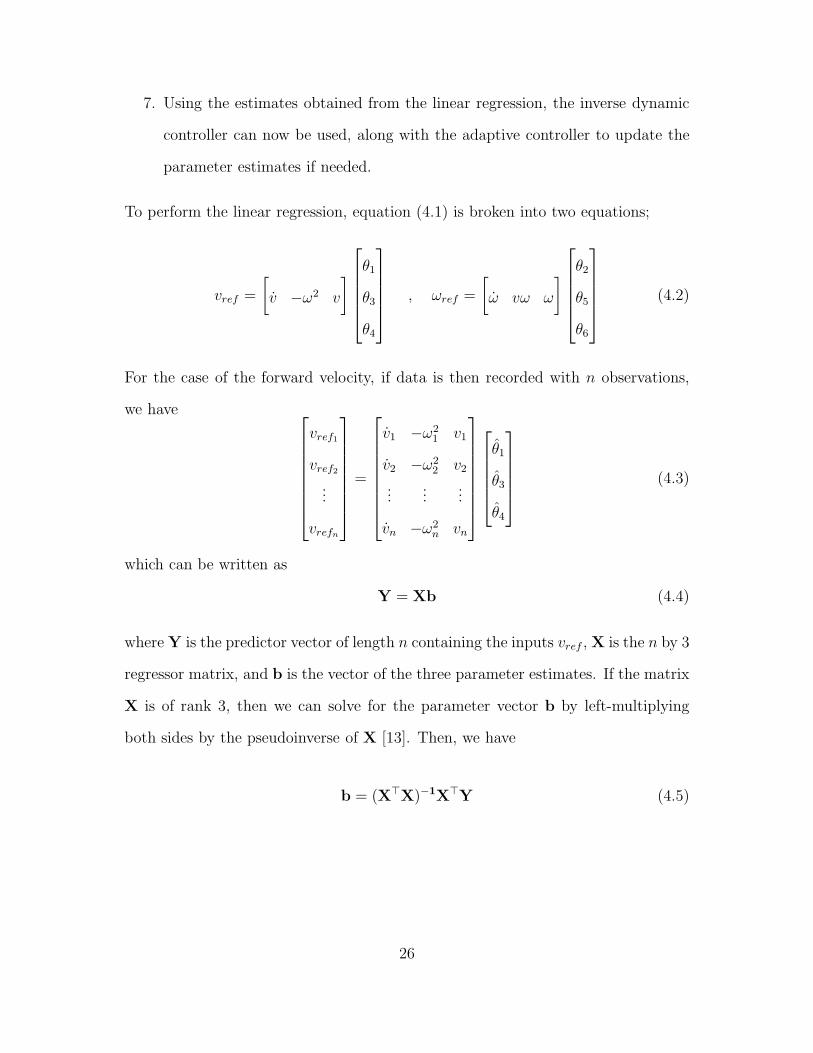
7. Using the estimates obtained from the linear regression, the inverse dynamic
controller can now be used, along with the adaptive controller to update the
parameter estimates if needed.
To perform the linear regression, equation (4.1) is broken into two equations;
vref =
[
v −ω2 v
]
θ1
θ3
θ4
, ωref =
[
ω vω ω
]
θ2
θ5
θ6
(4.2)
For the case of the forward velocity, if data is then recorded with n observations,
we have
vref1
vref2...
vrefn
=
v1 −ω21 v1
v2 −ω22 v2
......
...
vn −ω2n vn
θ1
θ3
θ4
(4.3)
which can be written as
Y = Xb (4.4)
whereY is the predictor vector of length n containing the inputs vref , X is the n by 3
regressor matrix, and b is the vector of the three parameter estimates. If the matrix
X is of rank 3, then we can solve for the parameter vector b by left-multiplying
both sides by the pseudoinverse of X [13]. Then, we have
b = (X⊤X)−1X⊤Y (4.5)
26
Page 35
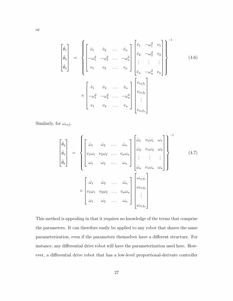
or
θ1
θ3
θ4
=
v1 v2 . . . vn
−ω21 −ω2
2 . . . −ω2n
v1 v2 . . . vn
v1 −ω21 v1
v2 −ω22 v2
......
...
vn −ω2n vn
−1
(4.6)
×
v1 v2 . . . vn
−ω21 −ω2
2 . . . −ω2n
v1 v2 . . . vn
vref1
vref2...
vrefn
Similarly, for ωref ,
θ2
θ5
θ6
=
ω1 ω2 . . . ωn
v1ω1 v2ω2 . . . vnωn
ω1 ω2 . . . ωn
ω1 v1ω1 ω1
ω2 v1ω2 ω2
......
...
ωn v1ωn ωn
−1
(4.7)
×
ω1 ω2 . . . ωn
v1ω1 v2ω2 . . . vnωn
ω1 ω2 . . . ωn
ωref1
ωref2
...
ωrefn
This method is appealing in that it requires no knowledge of the terms that comprise
the parameters. It can therefore easily be applied to any robot that shares the same
parameterization, even if the parameters themselves have a different structure. For
instance, any differential drive robot will have the parameterization used here. How-
ever, a differential drive robot that has a low-level proportional-derivate controller
27
Page 36
on forward and angular velocities will have parameters of a different form than one
that has proportional-derivate control on individual wheel velocities. Regardless of
this difference, since both robots share the same form of the parameterized model,
this method will work for both robots. This method can also be completely au-
tomated such that all the programmer needs to do is load the control algorithm
onto the robot. The robot can then perform the above steps on-board to obtain the
parameter estimates autonomously.
In a variation on the above approach, two of the parameters can first easily be ob-
tained. Observing equation (4.1), if the robot has only constant forward velocity
and a constant input vref , then we have a simple case where vref = θ4v. Similarly
for purely constant angular velocity, ωref = θ6ω. Intuitively, these values should be
close to unity, as we expect the robot’s low-level controller to achieve and maintain
the reference inputs. The robot can therefore be subjected to a constant forward
velocity, and after a steady-state velocity is reached, dividing vref by v will yield an
estimate for θ4. Doing the same for the angular velocity thereby produces two out
of the six unknown parameters.
28
Page 37
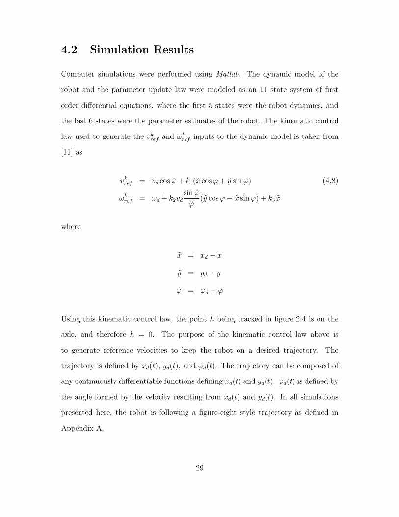
4.2 Simulation Results
Computer simulations were performed using Matlab. The dynamic model of the
robot and the parameter update law were modeled as an 11 state system of first
order differential equations, where the first 5 states were the robot dynamics, and
the last 6 states were the parameter estimates of the robot. The kinematic control
law used to generate the vkref and ωkref inputs to the dynamic model is taken from
[11] as
vkref = vd cos ϕ+ k1(x cosϕ+ y sinϕ) (4.8)
ωkref = ωd + k2vd
sin ϕ
ϕ(y cosϕ− x sinϕ) + k3ϕ
where
x = xd − x
y = yd − y
ϕ = ϕd − ϕ
Using this kinematic control law, the point h being tracked in figure 2.4 is on the
axle, and therefore h = 0. The purpose of the kinematic control law above is
to generate reference velocities to keep the robot on a desired trajectory. The
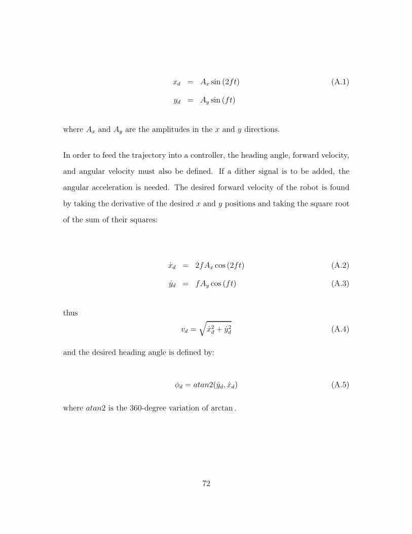
trajectory is defined by xd(t), yd(t), and ϕd(t). The trajectory can be composed of
any continuously differentiable functions defining xd(t) and yd(t). ϕd(t) is defined by
the angle formed by the velocity resulting from xd(t) and yd(t). In all simulations
presented here, the robot is following a figure-eight style trajectory as defined in
Appendix A.
29
Page 38
Simulations were performed to analyze the performance of the adaptive controller
in different scenarios. First, a simulation was run using perfect parameter estimates
and perfect initial conditions for position, but the robot having an initial velocity
of zero, which is not the initial desired velocity. Although the parameter estimates
begin at their true values, the values changed because of the error in initial velocity.
θ1, θ2, θ3, θ4, θ5, θ6
Figure 4.1: Legend for parameter evolution plots
distance error (θi = θ )
time [s]
error[m
]
0 1000 2000 3000 4000 5000 6000 70000
0.5
1
1.5
2
2.5
3×10⁻³
(a) Distance error
Evolution of adaptive terms ( θi = θi )
t [s]
θ
0 1000 2000 3000 4000 5000 6000 7000-0.2
0
0.2
0.4
0.6
0.8
1
1.2
(b) Parameter evolution
Figure 4.2: Perfect initial estimates
Figure 4.2(a) shows the error between the actual position and desired position along
the trajectory versus time for 50 iterations of the figure-eight trajectory. As time
increases the error decreases. In Figure 4.2(b), it can be observed that even though
the initial parameter estimates are perfect, they do not remain constant due to the
imperfect initial condition on velocity.
30
Page 39
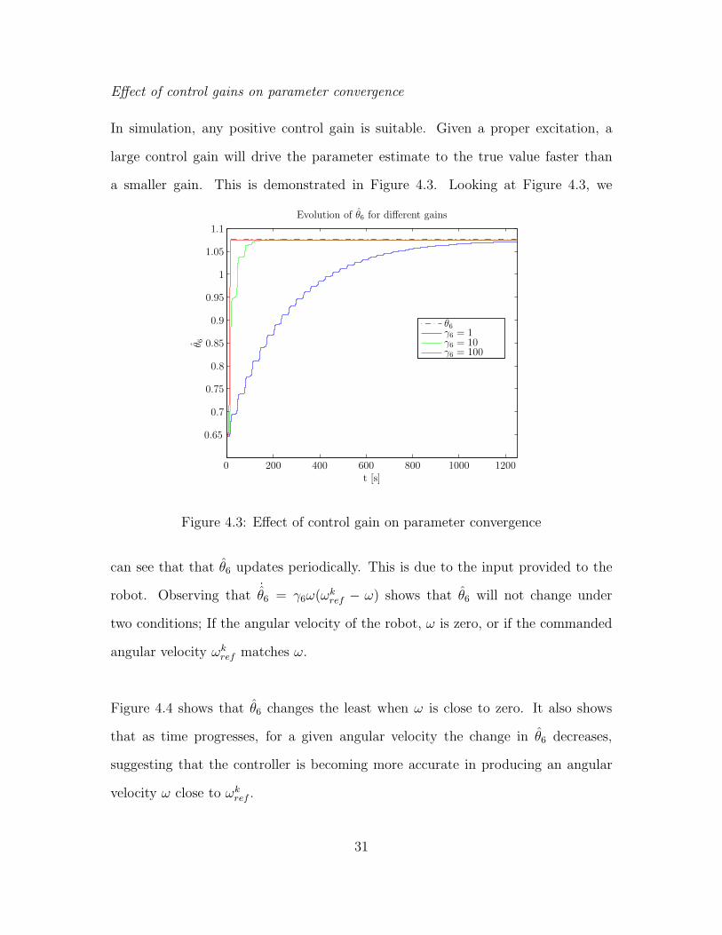
Effect of control gains on parameter convergence
In simulation, any positive control gain is suitable. Given a proper excitation, a
large control gain will drive the parameter estimate to the true value faster than
a smaller gain. This is demonstrated in Figure 4.3. Looking at Figure 4.3, we
Evolution of θ6 for different gains
t [s]
θ 6
θ6γ6 = 1γ6 = 10γ6 = 100
0 200 400 600 800 1000 1200
0.65
0.7
0.75
0.8
0.85
0.9
0.95
1
1.05
1.1
Figure 4.3: Effect of control gain on parameter convergence
can see that that θ6 updates periodically. This is due to the input provided to the
robot. Observing that˙θ6 = γ6ω(ω
kref − ω) shows that θ6 will not change under
two conditions; If the angular velocity of the robot, ω is zero, or if the commanded
angular velocity ωkref matches ω.
Figure 4.4 shows that θ6 changes the least when ω is close to zero. It also shows
that as time progresses, for a given angular velocity the change in θ6 decreases,
suggesting that the controller is becoming more accurate in producing an angular
velocity ω close to ωkref .
31
Page 40
ω and Evolution of θ6
t [s]
θ 6−
0.8,ω
ωθ6
0 200 400 600 800 1000 1200
-0.25
-0.2
-0.15
-0.1
-0.05
0
0.05
0.1
0.15
0.2
0.25
Figure 4.4: Angular velocity and θ6
Effect of input signal on parameter convergence
From the results in Figure 4.4, it is obvious that the input to the system has a
strong impact on the convergence of parameters. Here, the robot is again following
the figure-eight trajectory. For a given set of initial estimates, the parameters may
converge to different values in the case of different input signals. Below are examples
of two simulations with identical initial parameters and perfect initial conditions for
the position and velocity of the robot.
For the case of a simple figure-eight style trajectory, all terms except θ1 and θ5
approach their true values.
32
Page 41
Evolution of adaptive terms
t [s]
θ
0 200 400 600 800 1000 1200-0.2
0
0.2
0.4
0.6
0.8
1
1.2
Figure 4.5: Parameter evolution for figure-eight trajectory
θ initial final true1 0.4000 1.0291 0.26042 0.1000 0.3711 0.25093 0.7000 0.2847 -0.00044 0.3000 0.9539 0.99655 0.1000 0.1198 0.00266 0.6000 1.0779 1.0768
Table 4.1: Parameter final and initial values
33
Page 42
Evolution of adaptive terms
t [s]
θ
0 200 400 600 800 1000 1200-0.5
0
0.5
1
1.5
2
2.5
3
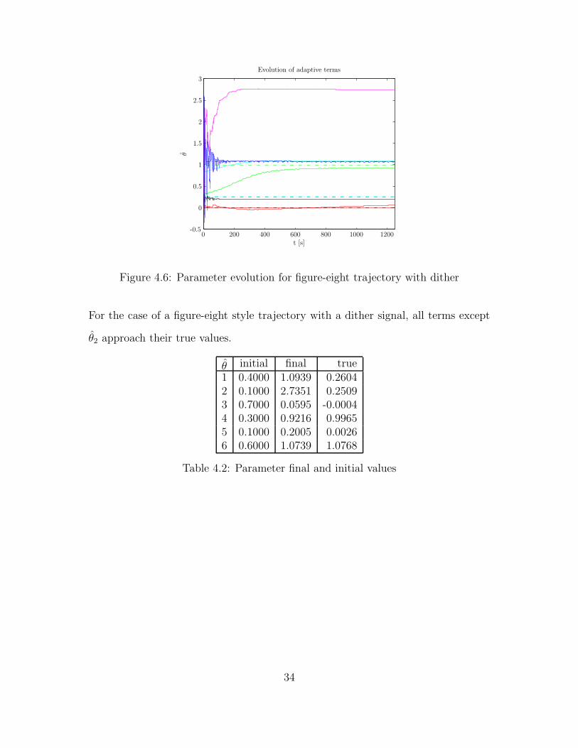
Figure 4.6: Parameter evolution for figure-eight trajectory with dither
For the case of a figure-eight style trajectory with a dither signal, all terms except
θ2 approach their true values.
θ initial final true1 0.4000 1.0939 0.26042 0.1000 2.7351 0.25093 0.7000 0.0595 -0.00044 0.3000 0.9216 0.99655 0.1000 0.2005 0.00266 0.6000 1.0739 1.0768
Table 4.2: Parameter final and initial values
34
Page 43
Effect of other parameters on parameter convergence
The convergence of a particular parameter can depend on the values of other pa-
rameters. This is demonstrated in the two simulations below.
Evolution of adaptive terms
t [s]
θ
0 200 400 600 800 1000 1200-0.2
0
0.2
0.4
0.6
0.8
1
1.2
Figure 4.7: Evolution of θ5
In Figure 4.7, all parameter estimates are perfect, except for θ5 (represented by the
solid black line). The only nonzero adaptive gain is γ5 = 10, such that only θ5 is
being updated. From the figure, we can see that θ5 is slowly approaching its true
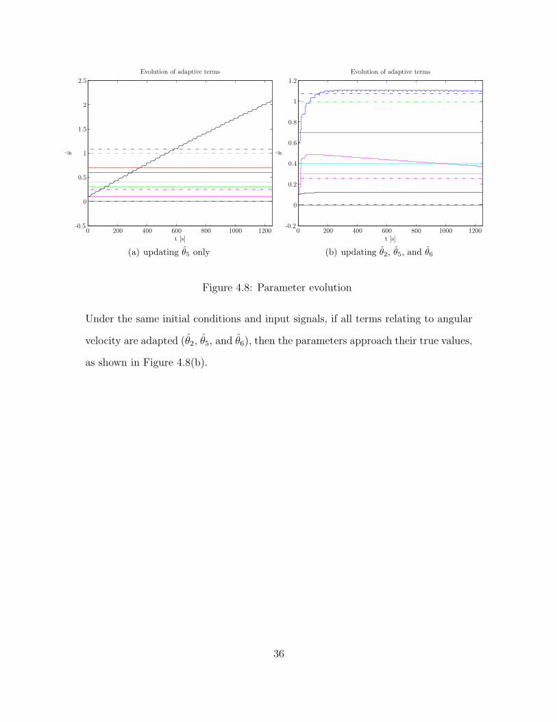
value. Figure 4.8(a) shows the evolution of θ5 for non-perfect parameter estimates,
with only θ5 being updated. In this case, θ5 moves away from its true value.
Considering that˙θ5 = γ5(ω
kref − ω), we know that
˙θ5 depends on ω. If we look at
the dynamic model of the robot, it can be seen that the angular velocity ω of the
robot contains the parameters θ2, θ5, and θ6. Thus if the estimates for θ2 and θ6
are inaccurate, and we try to adapt θ5, the value for θ5 may converge to some other
value to compensate for the error in angular velocity being produced due to the
inaccuracies in˙θ2 and
˙θ6
35
Page 44
Evolution of adaptive terms
t [s]
θ
0 200 400 600 800 1000 1200-0.5
0
0.5
1
1.5
2
2.5
(a) updating θ5 only
Evolution of adaptive terms
t [s]
θ
0 200 400 600 800 1000 1200-0.2
0
0.2
0.4
0.6
0.8
1
1.2
(b) updating θ2, θ5, and θ6
Figure 4.8: Parameter evolution
Under the same initial conditions and input signals, if all terms relating to angular
velocity are adapted (θ2, θ5, and θ6), then the parameters approach their true values,
as shown in Figure 4.8(b).
36
Page 45
Parameter projection
Since the parameters of the dynamic model represent combinations of physical con-
stants of the robot, most of which are known or can be estimated with some upper
and lower bound, bounds on the parameter estimates can be made. Using these
upper and lower bounds, the adaptive law can be modified to constrain each param-
eter estimate to remain within the predefined bounds [14].
If the following parameter update considered,
˙θi =
0 if θi ≥ θimaxand γig
⊤
iv > 0
γig⊤
iv if θimin
< θi < θimax
0 if θi ≤ θiminand γig
⊤
iv < 0
(4.9)
then the adaptive law is only active when each parameter is within its bounds.
Evolution of adaptive terms
t [s]
θ
0 20 40 60 80 100 120-0.5
0
0.5
1
1.5
2
2.5
3
(a) updating θ5 only
Evolution of adaptive terms
t [s]
θ
0 20 40 60 80 100 120-0.5
0
0.5
1
1.5
2
(b) updating θ2, θ5, and θ6
Figure 4.9: Parameter evolution
37
Page 46
The simulation results for the linear regression method proposed in section 4.1 are
shown in Figure 4.10. For the first case (Figures 4.10(a) and 4.10(b)), the system is
given an input signal of vref = 1 and ωref = 1. For the second case, the system was
given inputs of
vref = 0.2 sin (t) + 0.1 sin (1.5t) + 0.1 sin (3t) + 0.1 sin (0.1t) . . .
+ 0.08 sin (0.013t) + 0.1 sin (5t)
ωref = (5π/3) sin (2t) + 0.1 sin (0.1t) + 0.1 sin (0.09t)
38
Page 47
Linear regression
vω
v ref−θ 4v
-10
12
34
-2
0
2
4
-0.5
-0.5
0
0
0.5
0.5
1
(a) vref regression
vω
ωref−θ 6ω
-10
12
34
-2
0
2
4
-0.5
-0.5
0
0
0.5
0.5
1
(b) ωref regression
vω
v ref−θ 4v
-1-0.5
00.5
1
-10
-5
0
5
10-0.2
-0.1
0
0.1
0.2
0.3
(c) vref regression
vω
ωref−θ 6ω
-1-0.5
00.5
1
-10
-5
0
5
10
-4
-4
-2
-2
0
2
4
(d) ωref regression
Figure 4.10: Regression
39
Page 48
It was previously shown that the inputs provided to the dynamic model had a strong
impact on parameter convergence. In figure 4.10, this is shown for the case of linear
regression. It is clear that for the case where a more complex input signal is provided
(figures 4.10(c) and 4.10(d)), it is easier to define the surface that is created by the
datapoints. For this reason, when collecting data for a linear regression, a signal
that provides sufficient excitation should be chosen. In general, the signal should
contain at least half as many distinct frequencies as there are unknown parameters
[14].
40
Page 49
4.3 Experimental Setup
The proposed controller is tested on a Pioneer 3-DX and a Khepera III (figure 4.11).
The Pioneer 3-DX is a larger differential drive mobile robot, having a mass of 9 kilo-
grams. It has a maximum forward velocity of 1.4 meters per second, and a track
width of 34 centimeters. The Khepera III is a much smaller robot, with a mass of
742 grams. It has a maximum forward velocity of 500 millimeters per second, and a
track width of 89 millimeters. Because of the difference in size between these robots,
one can expect different dynamics between the two. Both robots take a forward and
angular reference velocity as inputs. It is worth noting that the Pioneer achieves the
reference velocities via proportional-derivative control on the forward and angular
velocities of the robot, whereas the Khepera III uses proportional-derivative control
on individual wheel velocities.
The Pioneer 3-DX has an onboard computer with a 1.8 GHz processor, 512 megabytes
of RAM and uses Debian Linux as an operating system. The Khepera III utilizes
a Gumstix Verdex computer-on-module operating at 600 MHz, with 128 megabytes
of RAM, and running OpenEmbedded Angstrom Linux as the operating system.
Since these two robots are made by different manufacturers, they do not use the
same libraries to interface the software with the hardware. For instance, the com-
mand to specify a forward velocity on the Pioneer 3-DX is not the same command
used on the Khepera III. A piece of software that addresses this issue is Player [15].
Player is a “cross-platform robot device interface” which provides a uniform inter-
face from robot to robot (provided that the robot is supported). Player is essentially
an additional layer of software on top of the basic libraries used to interface with
the robot. It is a very useful piece of software if the code being written is planned
to be used on multiple different platforms. Player also has the capability of being
41
Page 50
executed remotely. For instance, the program can be run on a base station, while
commanding motors and reading sensors by wireless internet. In the experiments
performed here, the program is run on the physical robot to eliminate any time de-
lays that may be associated with wireless communication. There is a disadvantage
of using player, namely the added computation time required. On the Pioneer 3-DX,
this is not much of an issue since it has a relatively fast processor. On the Khepera
III however, the sample time of the algorithm being implemented using Player is
about 0.8 second (compared to 0.3 second on the Pioneer 3-DX). For this reason,
using Player on the Khepera III is not a viable option. Instead, the Khepera III
toolbox is used. The Khepera III toolbox provides libraries, modules, and scripts for
interfacing with the Khepera III. Using the Khepera III toolbox decreased the sam-
ple time substantially to about 0.02 second. This does take away the convenience
of being able to run the same code on both robots, as was the case with Player.
Since the main advantage of using Player is now not applicable, there is no reason
to suffer the additional computational time in using it on the Pioneer. The pioneer
is therefore programmed in its native API, Aria. Information on programming in
Aria can be found in [16].
Figure 4.11: Khepera III and Pioneer 3-DX mobile robots
42
Page 51
In the experiments performed in the subsequent sections, all localization is based
off of each robot’s onboard odometry. During each iteration of the program, the
time elapsed from the start of the program is calculated. Based on the trajectory
programmed, the robot calculates a desired position, orientation, and velocity. This
data is recorded in a file desired. Each iteration, the robot also polls the encoders,
and calculates an estimate of its current position, which is stored in actual. From
the files desired and actual, plots of the desired and actual trajectories can be gen-
erated. Considering that the files store the x position in the first column, the y
position in the second column, and the orientation φ in the third column, a plot
of the trajectories can be generated in Matlab by executing the following commands;
load actual;
load desired;
plot(desired(:,1),desired(:,2),’-b’);
hold on
plot(actual(:,1),actual(:,2),’-r’);
The distance error is calculated by the following equation;
error =√
(xd − x)2 + (yd − y)2
The distance error is the main performance metric in the experiments performed,
and is what is trying to be minimized.
43
Page 52
4.4 Experimental Results
To demonstrate the necessity of generating reasonable initial parameter estimates
and the effectiveness of the proposed method for doing so, various experiments were
performed. The experiments were performed on two different robots, a Khepera III
and a Pioneer 3-DX. Both of these robots are similar in that they are differentially
driven, but differ in size. The difference in scale of the robots should add confidence
that the proposed method is effective regardless of the actual parameters being
estimated, and requires no modification to perform on different systems. To show
the effect of varying the dynamics of the robot, each robot is subject to a payload.
The adaptive control law will adjust the parameter estimates to compensate for the
change in dynamics introduced by the payload.
As discussed in Section 4.1, the values of θ4 and θ6 are expected to be close to 1. It
will be shown that both for the Khepera III and Pioneer 3-DX, the initial estimates
for these two parameters are indeed close to 1. If we observe the terms that comprise
each parameter (see Section 2.2), it should be noticed that the only parameters that
would be effected by an additional payload are θ1, θ2, θ3, and θ5, since these are the
only parameters that contain mass, inertia, and the location of the center of gravity.
Therefore, θ4 and θ6 can be held as constant during adaptation.
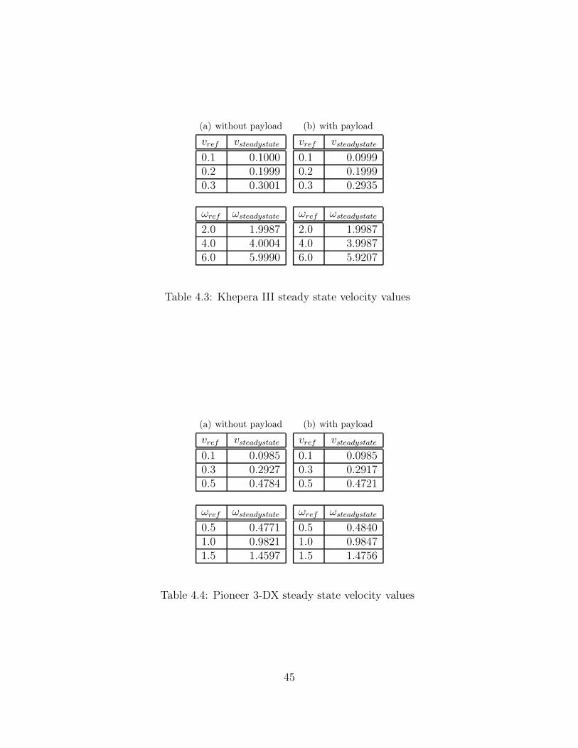
To further verify this assumption, each robot was subjected to various forward and
angular velocities, both with and without a payload. Comparing the steady-state
value with the reference value shows that the assumption is indeed valid.
44
Page 53
(a) without payload
vref vsteadystate
0.1 0.10000.2 0.19990.3 0.3001
ωref ωsteadystate
2.0 1.99874.0 4.00046.0 5.9990
(b) with payload
vref vsteadystate
0.1 0.09990.2 0.19990.3 0.2935
ωref ωsteadystate
2.0 1.99874.0 3.99876.0 5.9207
Table 4.3: Khepera III steady state velocity values
(a) without payload
vref vsteadystate
0.1 0.09850.3 0.29270.5 0.4784
ωref ωsteadystate
0.5 0.47711.0 0.98211.5 1.4597
(b) with payload
vref vsteadystate
0.1 0.09850.3 0.29170.5 0.4721
ωref ωsteadystate
0.5 0.48401.0 0.98471.5 1.4756
Table 4.4: Pioneer 3-DX steady state velocity values
45
Page 54
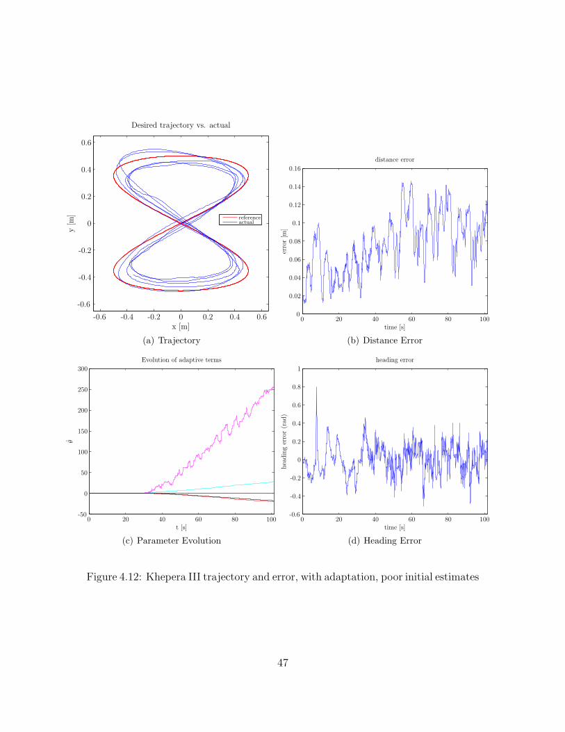
4.4.1 Khepera III
In simulation, it was shown that the initial parameter error does not need to be
small for the parameter estimates to converge. In reality, this is not the case. To
illustrate this, the adaptive controller was implemented on the Khepera III with all
initial parameter estimates chosen as 1. The robot is commanded to follow a figure-
eight style trajectory. At t = 30 seconds, the parameter adaptation begins. At this
time, it can be seen in figure 4.12(b) that the distance error begins to increase with
time, indicating a degradation in performance. Figure 4.12(c) shows the parameter
estimates. Although the true values are not known, it is clear that some of the
parameters are diverging quickly.
46
Page 55
Desired trajectory vs. actual
x [m]
y[m
]
referenceactual
-0.6 -0.4 -0.2 0 0.2 0.4 0.6
-0.6
-0.4
-0.2
0
0.2
0.4
0.6
(a) Trajectory
distance error
time [s]
error[m
]
0 20 40 60 80 1000
0.02
0.04
0.06
0.08
0.1
0.12
0.14
0.16
(b) Distance Error
Evolution of adaptive terms
t [s]
θ
0 20 40 60 80 100-50
0
50
100
150
200
250
300
(c) Parameter Evolution
heading error
time [s]
headingerror(rad
)
0 20 40 60 80 100-0.6
-0.4
-0.2
0
0.2
0.4
0.6
0.8
1
(d) Heading Error
Figure 4.12: Khepera III trajectory and error, with adaptation, poor initial estimates
47
Page 56
From the results shown in figure 4.12, it is obvious that a more intelligent estimate
of the initial parameters is needed. Using the method outlined in section 4.1, a more
reasonable initial estimate is generated.
First, the robot is given inputs of
vref = 0.1 + 0.05 sin (2t) + 0.05 sin (t) + 0.05 sin (t/3) + 0.05 sin (t/11)
ωref = 1.5 + 0.5 sin (3t/2) + 0.5 sin (t) + 0.25 sin (t/2) + 0.25 sin (t/5)
The forward and angular velocities were recorded by the robot as it moved. After 2
minutes, the robot was stopped and the data was collected. The velocity data was
filtered (figure 4.13)and differentiated to obtain the accelerations (figure 4.14).
t[s]
v
vv filtered
t[s]
ω
ωω filtered
0 20 40 60 80 100 120
0 20 40 60 80 100 120
-1
0
1
2
3
-0.1
0
0.1
0.2
0.3
Figure 4.13: Velocity data
48
Page 57
t[s]
vv from unfiltered datav from filtered data
t[s]
ω
ω from unfiltered dataω from filtered data
0 20 40 60 80 100 120
0 20 40 60 80 100 120
-10
-5
0
5
10
-0.5
0
0.5
Figure 4.14: Acceleration data
Although the velocity data of figure 4.13 doesn’t appear to be too noisy, it is obvious
that the acceleration data acquired by differentiating the noisy signal is useless.
Here, the data was filtered once forward, and again in reverse to eliminate any
added delay. The type of filter used was a Butterworth filter with a cutoff frequency
of 0.5 Hz. Using the filtered signals, a linear regression can be performed to obtain
estimates of the parameters.
49
Page 58
(a) vref regression (b) ωref regression
Figure 4.15: Plots of linear regression
Performing the linear regression as described in equations (4.6) and (4.7) on the
filtered signals, θ is found to be
θ1 = 0.0228
θ2 = 0.0568
θ3 = −0.0001
θ4 = 1.0030
θ5 = 0.0732
θ6 = 0.9981
As discussed in Section 4.1 (pg. 27), θ4 and θ6 were expected to be close to 1. Since
our values for these parameters obtained from the linear regression are close to 1,
this is a good indicator that the parameter estimates may be accurate.
50
Page 59
Desired trajectory vs. actual
x [m]
y[m
]
referenceactual
-0.6 -0.4 -0.2 0 0.2 0.4 0.6
-0.6
-0.4
-0.2
0
0.2
0.4
0.6
(a) Trajectory
distance error
time [s]
error[m
]
0 10 20 30 40 50 600
0.005
0.01
0.015
0.02
0.025
0.03
0.035
(b) Error
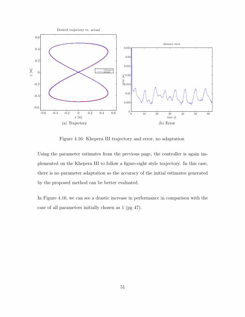
Figure 4.16: Khepera III trajectory and error, no adaptation
Using the parameter estimates from the previous page, the controller is again im-
plemented on the Khepera III to follow a figure-eight style trajectory. In this case,
there is no parameter adaptation so the accuracy of the initial estimates generated
by the proposed method can be better evaluated.
In Figure 4.16, we can see a drastic increase in performance in comparison with the
case of all parameters initially chosen as 1 (pg 47).
51
Page 60
Desired trajectory vs. actual
x [m]
y[m
]
referenceactual
-0.6 -0.4 -0.2 0 0.2 0.4 0.6
-0.6
-0.4
-0.2
0
0.2
0.4
0.6
(a) Trajectory
distance error
time [s]
error[m
]
0 50 100 1500
0.005
0.01
0.015
0.02
0.025
0.03
0.035
(b) Distance Error
Evolution of adaptive terms
t [s]
θ
0 50 100 150-0.2
0
0.2
0.4
0.6
0.8
1
1.2
(c) Parameter Evolution
heading error
time [s]
headingerror(rad
)
0 50 100 150-0.08
-0.06
-0.04
-0.02
0
0.02
0.04
0.06
0.08
(d) Heading Error
Figure 4.17: Khepera III trajectory and error, with adaptation
52
Page 61
Although in Figure 4.16, the performance of the controller is acceptable with using
the initial parameter estimates, and no parameter adaptation, there is still room for
improvement. Figure 4.17 shows the same scenario, but with adaptation beginning
at t = 3 seconds. A slight decrease in distance error can be noticed, along with
a small change in the parameter estimates. A comparison of the errors in the two
scenarios is shown in Figure 4.18.ts
distance error
time [s]
error[m
]
not adaptingadapting
0 10 20 30 40 50 600
0.005
0.01
0.015
0.02
0.025
0.03
0.035
(a) Distance Error
heading error
time [s]
headingerror(rad
)
not adaptingadapting
0 10 20 30 40 50 60-0.1
-0.08
-0.06
-0.04
-0.02
0
0.02
0.04
0.06
0.08
(b) Heading Error
Figure 4.18: Comparison of figures 4.16 and 4.17
53
Page 62
Desired trajectory vs. actual
x [m]
y[m
] referenceactual
-1 -0.8 -0.6 -0.4 -0.2 0 0.2 0.4 0.6 0.8
-0.6
-0.4
-0.2
0
0.2
0.4
0.6
0.8
(a) Trajectory
distance error
time [s]
error[m
]
0 5 10 15 20 25 300
0.1
0.2
0.3
0.4
0.5
0.6
0.7
0.8
0.9
1
(b) Error
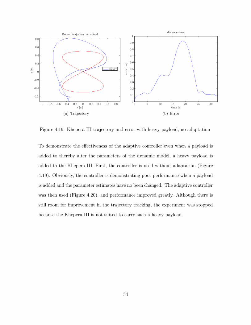
Figure 4.19: Khepera III trajectory and error with heavy payload, no adaptation
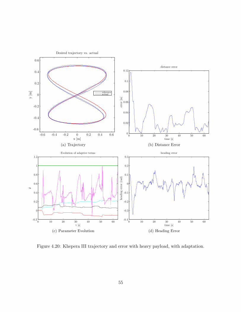
To demonstrate the effectiveness of the adaptive controller even when a payload is
added to thereby alter the parameters of the dynamic model, a heavy payload is
added to the Khepera III. First, the controller is used without adaptation (Figure
4.19). Obviously, the controller is demonstrating poor performance when a payload
is added and the parameter estimates have no been changed. The adaptive controller
was then used (Figure 4.20), and performance improved greatly. Although there is
still room for improvement in the trajectory tracking, the experiment was stopped
because the Khepera III is not suited to carry such a heavy payload.
54
Page 63
Desired trajectory vs. actual
x [m]
y[m
]
referenceactual
-0.6 -0.4 -0.2 0 0.2 0.4 0.6
-0.6
-0.4
-0.2
0
0.2
0.4
0.6
(a) Trajectory
distance error
time [s]
error[m
]
0 10 20 30 40 50 600
0.02
0.04
0.06
0.08
0.1
0.12
(b) Distance Error
Evolution of adaptive terms
t [s]
θ
0 10 20 30 40 50 60-0.2
0
0.2
0.4
0.6
0.8
1
1.2
(c) Parameter Evolution
heading error
time [s]
headingerror(rad
)
0 10 20 30 40 50 60-0.4
-0.3
-0.2
-0.1
0
0.1
0.2
0.3
(d) Heading Error
Figure 4.20: Khepera III trajectory and error with heavy payload, with adaptation.
55
Page 64
Desired trajectory vs. actual
x [m]
y[m
]
referenceactual
-0.6 -0.4 -0.2 0 0.2 0.4 0.6
-0.6
-0.4
-0.2
0
0.2
0.4
0.6
(a) Trajectory
distance error
time [s]
error[m
]
0 10 20 30 40 50 60 700
0.02
0.04
0.06
0.08
0.1
0.12
0.14
0.16
0.18
(b) Error
Figure 4.21: Khepera III trajectory and error with light payload, no adaptation.
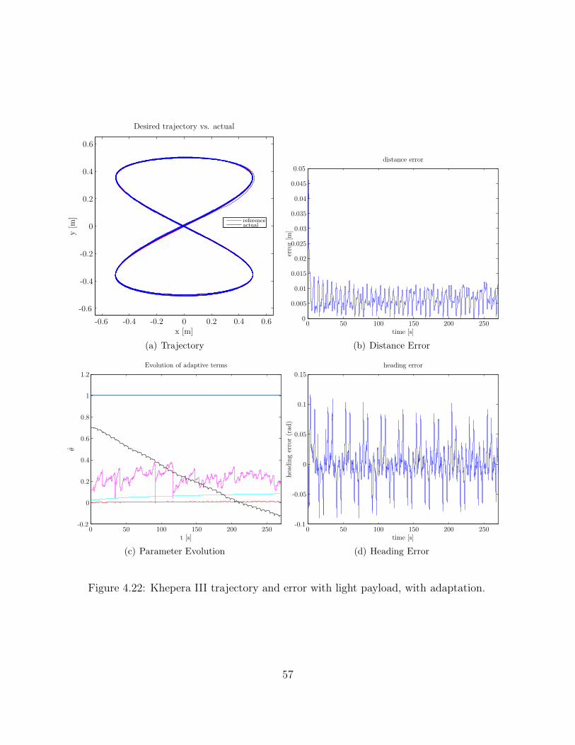
The Khepera III then had a lighter payload attached, and the initial parameter
estimates were again generated using the proposed method to demonstrate that it is
effective under different loading conditions using the same input signals and method
performed initially (page 48). First, the robot with the light payload was controlled
using the initial estimates without adaptation, as shown in Figure 4.21. Here, the
controller is performing well, again showing that the initial parameter estimate gen-
erated by the proposed method is accurate.
The experiment was then executed again using adaptation, and an increase in per-
formance is noticed (Figure 4.22).
56
Page 65
Desired trajectory vs. actual
x [m]
y[m
]
referenceactual
-0.6 -0.4 -0.2 0 0.2 0.4 0.6
-0.6
-0.4
-0.2
0
0.2
0.4
0.6
(a) Trajectory
distance error
time [s]
error[m
]
0 50 100 150 200 2500
0.005
0.01
0.015
0.02
0.025
0.03
0.035
0.04
0.045
0.05
(b) Distance Error
Evolution of adaptive terms
t [s]
θ
0 50 100 150 200 250-0.2
0
0.2
0.4
0.6
0.8
1
1.2
(c) Parameter Evolution
heading error
time [s]
headingerror(rad
)
0 50 100 150 200 250-0.1
-0.05
0
0.05
0.1
0.15
(d) Heading Error
Figure 4.22: Khepera III trajectory and error with light payload, with adaptation.
57
Page 66
distance error
time [s]
error[m
]
not adaptingadapting
0 10 20 30 40 50 60 700
0.02
0.04
0.06
0.08
0.1
0.12
0.14
0.16
0.18
(a) Trajectory
heading error
time [s]
headingerror(rad
)
not adaptingadapting
0 10 20 30 40 50 60 70-0.4
-0.3
-0.2
-0.1
0
0.1
0.2
0.3
(b) Distance Error
Figure 4.23: Comparison of Figures 4.21 and 4.22
58
Page 67
4.4.2 Pioneer 3-DX
As with the Khepera III, we first demonstrate the with poor initial estimates for
the parameters, the parameters may not converge. In Figure 4.24, all parameter
estimates are initially one. Again, this shows that a more intelligent initial estimate
is needed.
59
Page 68
Desired trajectory vs. actual
x [m]
y[m
]
referenceactual
-2 -1 0 1 2
-2
-1.5
-1
-0.5
0
0.5
1
1.5
2
(a) Trajectory
distance error
time [s]
error[m
]
0 20 40 60 80 100 120 140 1600
0.1
0.2
0.3
0.4
0.5
0.6
0.7
(b) Error
Evolution of adaptive terms
t [s]
θ
0 20 40 60 80 100 120 140 160-5
0
5
10
15
20
25
30
35
(c) Parameter Evolution
heading error
time [s]
headingerror(rad
)
0 20 40 60 80 100 120 140 160-0.2
-0.15
-0.1
-0.05
0
0.05
0.1
0.15
0.2
(d) Heading Error
Figure 4.24: Pioneer 3-DX trajectory and error, poor initial estimates, with adap-tation.
60
Page 69
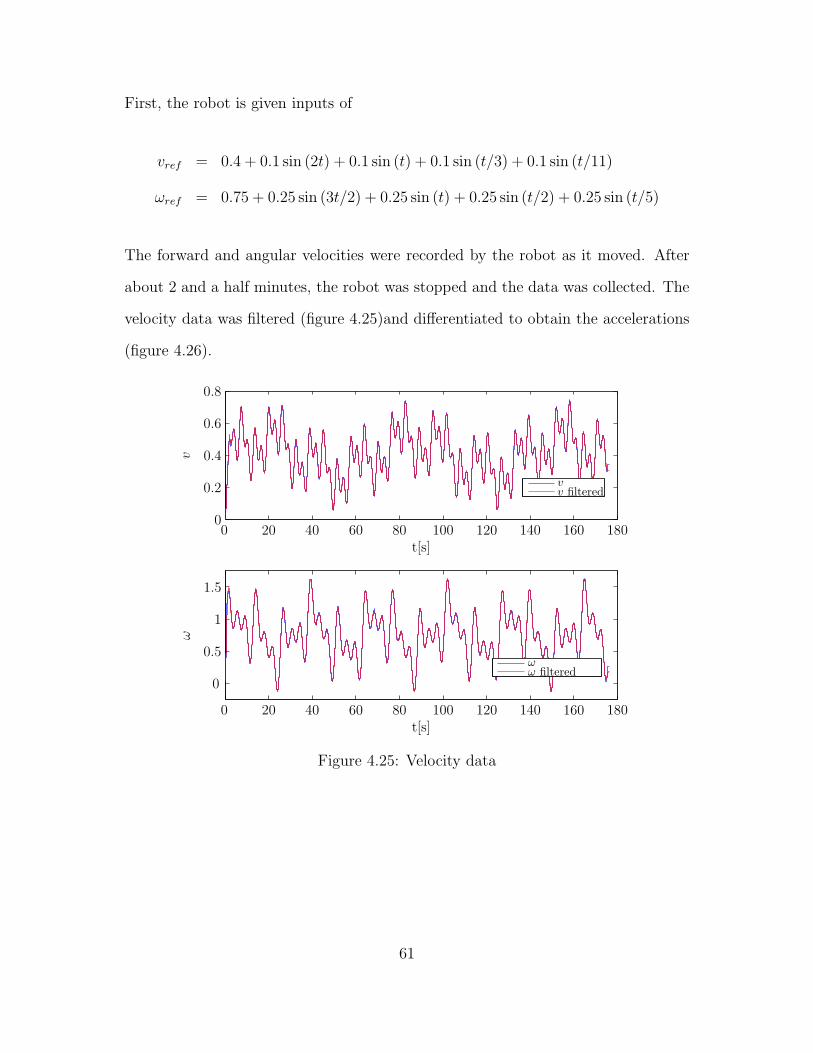
First, the robot is given inputs of
vref = 0.4 + 0.1 sin (2t) + 0.1 sin (t) + 0.1 sin (t/3) + 0.1 sin (t/11)
ωref = 0.75 + 0.25 sin (3t/2) + 0.25 sin (t) + 0.25 sin (t/2) + 0.25 sin (t/5)
The forward and angular velocities were recorded by the robot as it moved. After
about 2 and a half minutes, the robot was stopped and the data was collected. The
velocity data was filtered (figure 4.25)and differentiated to obtain the accelerations
(figure 4.26).
t[s]
v
vv filtered
t[s]
ω
ωω filtered
0 20 40 60 80 100 120 140 160 180
0 20 40 60 80 100 120 140 160 180
0
0.5
1
1.5
0
0.2
0.4
0.6
0.8
Figure 4.25: Velocity data
61
Page 70
t[s]
vv from unfiltered datav from filtered data
t[s]
ω
ω from unfiltered dataω from filtered data
0 20 40 60 80 100 120 140 160 180
0 20 40 60 80 100 120 140 160 180
-2
-1
0
1
2
-0.5
0
0.5
Figure 4.26: Acceleration data
Again, the velocity data of figure 4.25 doesn’t appear to be too noisy, but the
acceleration data derived from the raw velocities is not good. This demonstrates
the importance of filtering any signal before differentiating it. The data was filtered
the same way as the case for the Khepera, once forward, and again in reverse to
eliminate any added delay using a Butterworth filter with a cutoff frequency of
0.5 Hz. Using the filtered signals, a linear regression can be performed to obtain
estimates of the parameters.
62
Page 71
(a) vref regression (b) ωref regression
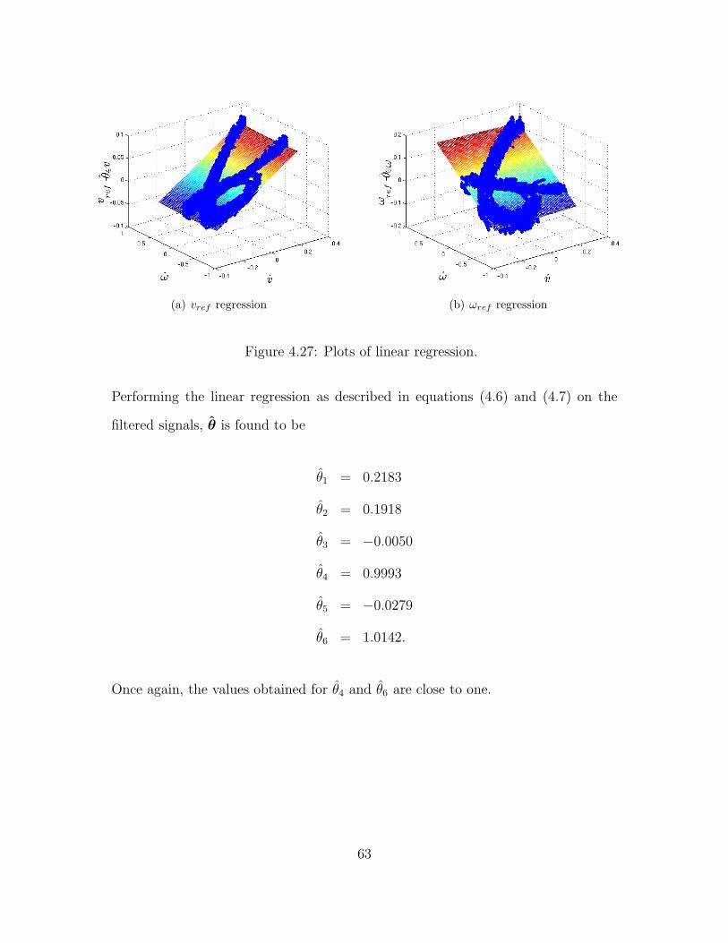
Figure 4.27: Plots of linear regression.
Performing the linear regression as described in equations (4.6) and (4.7) on the
filtered signals, θ is found to be
θ1 = 0.2183
θ2 = 0.1918
θ3 = −0.0050
θ4 = 0.9993
θ5 = −0.0279
θ6 = 1.0142.
Once again, the values obtained for θ4 and θ6 are close to one.
63
Page 72
In Figure 4.28, the Pioneer 3-DX is using the parameter estimates generated by the
proposed method, and at t = 30 seconds, adaptation begins. Only a small decrease
in the distance error can be noticed, suggesting that initial parameter estimates are
decent. Viewing Figure 4.28(c), the parameters quickly converge to new values not
far from the initial estimates.
64
Page 73
Desired trajectory vs. actual
x [m]
y[m
]
referenceactual
-2 -1 0 1 2
-2
-1.5
-1
-0.5
0
0.5
1
1.5
2
(a) Trajectory
distance error
time [s]
error[m
]
0 50 100 150 200 2500
0.1
0.2
0.3
0.4
0.5
0.6
0.7
(b) Error
Evolution of adaptive terms
t [s]
θ
0 50 100 150 200 250-0.2
0
0.2
0.4
0.6
0.8
1
1.2
(c) Parameter Evolution
heading error
time [s]
headingerror(rad
)
0 50 100 150 200 250-0.2
-0.15
-0.1
-0.05
0
0.05
0.1
0.15
(d) Heading Error
Figure 4.28: Pioneer 3-DX trajectory and error, adapting all parameters except θ4and θ6
65
Page 74
Desired trajectory vs. actual
x [m]
y[m
]
referenceactual
-2 -1 0 1 2
-2
-1.5
-1
-0.5
0
0.5
1
1.5
2
(a) Trajectory
distance error
time [s]
error[m
]
0 50 100 150 200 2500
0.1
0.2
0.3
0.4
0.5
0.6
0.7
(b) Error
heading error
time [s]
headingerror(rad
)
0 10 20 30 40 50 60-0.2
-0.15
-0.1
-0.05
0
0.05
0.1
0.15
(c) Heading Error
Figure 4.29: Pioneer 3-DX trajectory and error, heavy payload, no adaptation .
66
Page 75
The Pioneer 3-DX was then subjected to a heavy payload. The results of tracking
a figure-eight trajectory using the inverse dynamic controller with the estimates for
the robot with no payload without adaptation are shown in Figure 4.29.
The same scenario was performed again using adaptation, shown in Figure 4.30.
Again, there is a slight improvement in performance after updating is enabled at
t = 30 seconds, and the parameters quickly converge to new values. It should also
be noted that a payload has less of an effect on the larger robot than the smaller
one, where the Khepera III was not even able to track a trajectory when a large
payload was placed on it.
67
Page 76
Desired trajectory vs. actual
x [m]
y[m
]
referenceactual
-2 -1 0 1 2
-2
-1.5
-1
-0.5
0
0.5
1
1.5
2
(a) Trajectory
distance error
time [s]
error[m
]
0 50 100 1500
0.1
0.2
0.3
0.4
0.5
0.6
0.7
(b) Error
Evolution of adaptive terms
t [s]
θ
0 50 100 150-0.2
0
0.2
0.4
0.6
0.8
1
1.2
(c) Parameter Evolution
heading error
time [s]
headingerror(rad
)
0 50 100 150-0.2
-0.15
-0.1
-0.05
0
0.05
0.1
0.15
(d) Heading Error
Figure 4.30: Pioneer 3-DX trajectory and error, heavy payload, with adaptation .
68
Page 77
Chapter 5
Conclusions and Future Work
5.1 Conclusions
In this work, a review of the kinematics and dynamics of a differential drive wheeled
mobile robot was given. An adaptive controller for the parameters of the dynamic
model was also studied. In the physical implementation of the adaptive controller
based on the dynamic model, it was noticed that the accuracy of the initial estimate
of the parameters is important for the convergence of the parameter estimates, as
well as the performance of the inverse dynamic controller. A method for generating
an initial parameter estimate was proposed. The estimate was created by giving
the robot forward and angular reference velocities, collecting the actual velocities,
and performing a linear regression on the data. This method allowed for use on
different robotic platforms, and provided acceptable initial estimates. Experimen-
tal results, performed on two differentially-driven mobile robots, showed that the
proposed method is effective in generating initial estimates. The method proposed
here is attractive in that it requires absolutely no knowledge of what the parameters
might be, and can easily be implemented on platforms of whose parameters are very
69
Page 78
different, without any adjustment.
5.2 Future Work
In this work, a robot was given input signals, and data was collected. The initial
parameters were then generated on a separate computer. For future work, the ini-
tial parameter estimation should be completely autonomously by the robot. The
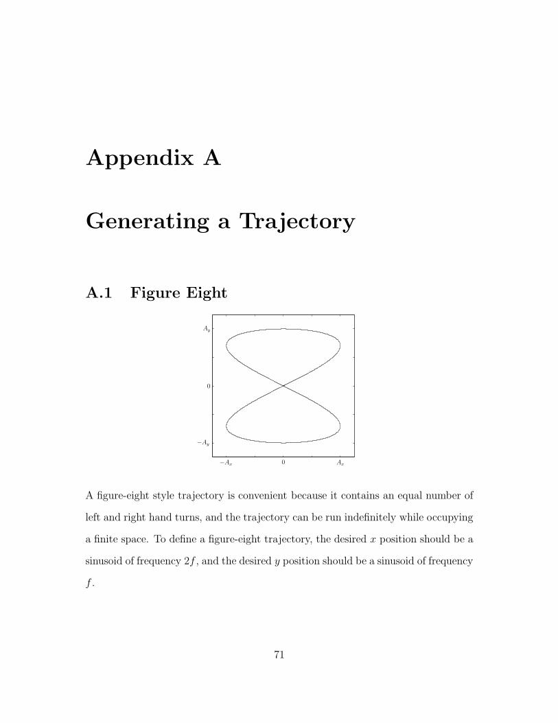
controller applied in the experimental results section did not use any form of satu-
ration control, so extra care was taken when generating trajectories so the robot’s
actuators would not saturate. An improvement to the current controller would be
to incorporate saturation control. The excitation signals used when collecting data
for the linear regression were chosen empirically, but it is suspected that there ex-
ist excitation signals that would allow for the identification of the parameters in a
minimum amount of time. Performing the linear regression with projection, using
information as to what the range of parameter estimates may be, could possibly
yield more accurate initial estimates.
70
Page 79
Appendix A
Generating a Trajectory
A.1 Figure Eight
−Ax 0 Ax
−Ay
0
Ay
A figure-eight style trajectory is convenient because it contains an equal number of
left and right hand turns, and the trajectory can be run indefinitely while occupying
a finite space. To define a figure-eight trajectory, the desired x position should be a
sinusoid of frequency 2f , and the desired y position should be a sinusoid of frequency
f .
71
Page 80
xd = Ax sin (2ft) (A.1)
yd = Ay sin (ft)
where Ax and Ay are the amplitudes in the x and y directions.
In order to feed the trajectory into a controller, the heading angle, forward velocity,
and angular velocity must also be defined. If a dither signal is to be added, the
angular acceleration is needed. The desired forward velocity of the robot is found
by taking the derivative of the desired x and y positions and taking the square root
of the sum of their squares:
xd = 2fAx cos (2ft) (A.2)
yd = fAy cos (ft) (A.3)
thus
vd =√
x2d + y2d (A.4)
and the desired heading angle is defined by:
φd = atan2(yd, xd) (A.5)
where atan2 is the 360-degree variation of arctan .
72
Page 81
Similarly, the desired accelerations and jerks are:
xd = −4f 2Ax sin (2ft) (A.6)
yd = −f 2Ay sin (ft) (A.7)
(A.8)
...x d = −8f 3Ax cos (2ft) (A.9)
...y d = −f 3Ay cos (ft) (A.10)
The desired angular velocity and acceleration are defined as follows:
ωd =ydxd − xdydx2d + y2d
(A.11)
αd =(...y dxd −
...x dyd)(x
2d + y2d)− (ydxd − xdyd)(2xdxd + 2ydyd)
(x2d + y2d)2
(A.12)
A.2 Figure Eight with Dither
The dither signal is added to the robot’s local x coordinate, and can be defined as:
d = g sin (ht) cos (kt)elt (A.13)
In order to add the dither signal to a trajectory, the first and second derivatives
73
Page 82
must be known, and are:
d = g[h cos (ht) cos (kt)− k sin (ht) sin (kt) + l sin (ht) cos (kt)]elt (A.14)
d = g[(l2 − h2 − k2) sin (ht) cos (kt)− 2hk cos (ht) sin (kt) + (A.15)
2hl cos (ht) cos (kt)− 2kl sin (ht) sin (kt)]elt (A.16)
The desired position with dither can then be defined as:
xddither = xd + d cos (π
2− φd) (A.17)
= xd + d sinφd (A.18)
(A.19)
yddither = yd + d sin (π
2− φd) (A.20)
= yd + d cosφd (A.21)
The remainder of the necessary parameters are found as they were previously:
xddither = xd + d sin φd + dωd cosφd (A.22)
yddither = yd + d cos φd − dωd sinφd (A.23)
vddither =√
x2ddither + y2ddither (A.24)
φddither = atan2(yddither , xddither) (A.25)
74
Page 83
xddither = xd + d sinφd + 2dωd cosφd − dω2d sin φd (A.26)
yddither = yd + d cosφd − 2dωd sinφd − dω2d cosφd (A.27)
ωddither =yddither xddither − xddither yddither
x2ddither + y2ddither(A.28)
−Ax 0 Ax
−Ay
0
Ay
75
Page 84
A.3 Alterative Parameterized Dynamic Model
Referring to pages 8 and 9 for the list of terms of the dynamic model, and the rest
of the derivation in section 2.2, the parameterized dynamic model for a differential
drive wheeled mobile robot with proportional-derivative gains on the forward and
angular velocties is obtained with some changes.
First, equation (2.11) is changed to
vv
vω
=
KPT (vref − vme)−KDT vme
KPR(ωref − ωme)−KDRωme
(A.29)
with
vme =1
2[r(ωr + ωl)] ωme =
1
d[r(ωr − ωl)] (A.30)
vv =vl + vr
2vω =
vr − vl2
(A.31)
where vme and ωme are the measured forward and angular velocities, and vref and
ωref are the commanded forward and angular velocities. The derivatives of the com-
manded velocities were neglected.
Now, the parameterized dynamic model is solved similar to section 2.2
From the second and third equations of (2.6) we can solve for the angular accelera-
tion,
ω =d
2Iz(Frrx′ − Frlx′) +
e
IzFey′ +
c
IzFcy′ +
1
Izτe −
mb
Iz( ˙v + vω) (A.32)
76
Page 85
Combining equations (2.9) and (2.10),
Frrx′ =ka
RaRt
(vr − kbωr)−IeRt
ωr −Be
Rt
ωr (A.33)
Frlx′ =ka
RaRt
(vl − kbωl)−IeRt
ωl −Be
Rt
ωl
And from equation (2.9),
ωr + ωl =2
rv −
1
r(vsr + vsl ) (A.34)
ωr − ωl =d
rω −
1
r(vsr − vsl )
The above equation along with (A.29) gives,
vr + vl = 2kPT
(
vref − v +1
2(vsr + vsl )
)
− 2kDT
(
v −1
2(vsr + vsl )
)
(A.35)
vr − vl = 2kPR
(
ωref − ω +1
d(vsr − vsl )
)
− 2kDR
(
ω −1
d(vsr − vsl )
)
The lateral velocity is found from the second and third equations of (2.8) as,
v = bω + vs (A.36)
Combining the lateral forces acting on each wheel (equation (2.13)) and the angular
acceleration (equation (A.32)), and using the second equations of (A.34) and (A.35)
77
Page 86
as well as the above equation for lateral velocity,
θ2ω = ωref − θ6ω +1
dθ6(v
sr − vsl ) +
(
kDR
dkPR
+RaIe
2kPRkar
)
(vsr − vsl ) +
RaRt
dkPRka(eFey′ + cFcy′ + τe)− θ5 ˙v
s − θ5vω (A.37)
Similarly, using the lateral forces, the sum of forces about the x′ axis, and the first
equations of (A.34) and (A.35) with (A.36),
θ1v = vref − θ4v +1
2θ4(v
sr + vsl ) +
(
kDT
2kPT
+RaIe
2kPTkar
)
(vsr + vsl ) +
RaRt
2kPTka(Fex′ + Fcx′) + θ3ω
2 +RaRtm
2kPTkaωvs (A.38)
The combination of equations (A.36) and (2.7), along with the above two equations
gives the dynamic model,
x
y
ψ
v
ω
=
v cosψ − aω sinψ
v sinψ + aω cosψ
ω
θ3θ1ω2 − θ4
θ1v
−θ5θ2vω − θ6
θ2ω
+
0 0
0 0
0 0
1θ1
0
0 1θ2
vref
ωref
+
δx
δy
0
δv
δω
(A.39)
78
Page 87
with
θ1 =
(
Ra
ka
)
/(2rkPT )
θ2 =
(
Ra
ka(Ied
2 + 2Rtr(Iz +mb2)) + 2rdkDR
)
/(2rdkPR)
θ3 =Ra
kambRt/(2kPT )
θ4 =Ra
ka
(
kakbRa
+Be
)
/(rkPT ) + 1
θ5 =Ra
kambRt/(dkPR)
θ6 =Ra
ka
(
kakbRa
+Be
)
d/(2rkPR) + 1
79
Page 88
Appendix B
Installing and Using the Khepera
III Toolbox
B.1 Installing the toolbox
The Khepera III toolbox requires nothing to be done onboard the Khepera.
First, download the latest revision of the toolbox;
svn checkout https://khepera3toolbox.svn.sourceforge.net/svnroot/khepera3toolbox
The Khepera III toolbox is now installed in the directory in which svn was run.
The following environment variables need to be added to ~/.bashrc.
First, type
vi ~/.bashrc
Then, at the bottom of the file, add
export K3 ROOT=/path/to/your/khepera3toolbox
80
Page 89
export PATH=$PATH:$K3 ROOT/Scripts
A new terminal window will need to be opened for bash to recognize the new environ-
ment variables (alternatively, the user can just type bash in the current terminal).
B.2 Writing a program
First, the cross-compiler for the ARM architecture must be installed. This is
availeble from K-team’s website by downloading the Korebot toolchain. Once
the toolchain is downloaded, the path to the ARM compiler must be added to
~/.bashrc. In ~/.bashrc, add
export PATH=$PATH:/path/to/your/arm/toolchain/bin
Now, to make a new program, in the Programs directory of the Khepera III toolbox,
type
k3-create-program program name
where program name is the name of the program you wish to create. Doing this cre-
ates a template file in C with all of the necessary header files, as well as a makefile
within a directory named after the program just created. Entering the directory of
the program and typing make builds the program.
The program can be placed on the Khepera by typing
k3put +ip address program name
Where ip address is the IP address of the Khepera III robot being used.
81
Page 90
Bibliography
[1] F. D. Boyden and S. A. Velinsky, “Dynamic modeling of wheeled mobile robotsfor high load applications,” in IEEE International conference on Robotics and
Automation, August 2002.
[2] T. Fukao, H. Nakagawa, and N. Adachi, “Adaptive tracking control of a non-holonomic mobile robot,” in IEEE Transactions on Robotics and Automation,October 2000.
[3] M. S. Kim, J. H. Shin, and J. J. Lee, “Design of a robust adaptive controller fora mobile robot,” in Internation Conference on Intelligent Robots and Systems,2000.
[4] R. Fierro and F. L. Lewis, “Control of a nonholonomic mobile robot: Backstep-ping kinematics into dynamics,” Journal of Robotic Systems, vol. 14, pp. 149–163, 1997.
[5] Y. Zhang, D. Hong, J. H. Chung, and S. Velinsky, “Dynamic model basedrobust tracking control of a differentially steered wheeled mobile robot,” inProceedings of the American Control Conference, June 1998.
[6] J. S. Choi and B. K. Kim, “Near minimum-time direct voltage control algo-rithms for wheeled mobile robots with current and voltage constraints,” inRobotica, 2001.
[7] R. Rajagopalan and N. Barakat, “Velocity control of wheeled mobile robotsusing computed torque control and its performance for a differentially drivenrobot,” Journal of Robotic Systems, vol. 14, pp. 325–340, 1997.
[8] C. D. L. Cruz and R. Carelli, “Dynamic model based formation control andobstacle avoidance of multi-robot systems,” Robotica, vol. 26, pp. 345–356,2008.
[9] B. Siciliano, L. Sciavicco, L. Villani, and G. Oriolo, Robotics; Modelling, Plan-
ning and Control. London, England: Springer-Verlag, 2009.
[10] G. Dudek and M. Jenkin, Handbook of Robotics, ch. 20, Inertial Sensors, GPS,and Odometry. Springer-Verlag, 2008.
82
Page 91
[11] G. Oriolo, A. D. Luca, and M. Vendittelli, “Wmr control via dynamic feedbacklinearization: design, implementation, and experimental validation,” in IEEE
Transactions on Control Systems Technology, November 2002.
[12] F. N. Martins, W. C. Celeste, and R. Carelli, “An adaptive dynamic controllerfor autonomous mobile robot trajectory tracking,” Control Engineering Prac-
tice, vol. 16, pp. 1354–1363, 2008.
[13] N. R. Draper and H. Smith, Applied regression analysis. New York, New York:John Wiley & Sons, 1998.
[14] P. Ioannou and J. Sun, Robust Adaptive Control. Prentice Hall, 1995.
[15] “Player/stage.” http://playerstage.sourceforge.net/, May 2011.
[16] A. Whitbrook, Programming mobile robots with Aria and Player. London,England: Springer-Verlag, 2010.
[17] F. Reyes and R. Kelly, “On parameter identification of robot manipulators,”in Proceedings of the 1997 IEEE international conference on robotics and au-
tomation, April 1997.
[18] G. Campion, G. Bastin, and B. D’andrea-Novel, “Structural properties andclassification of kinematic and dynamic models of wheeled mobile robots,” inIEEE Transactions on Robotics and Automation, February 1996.
[19] “Khepera iii toolbox.” http://en.wikibooks.org/wiki/Khepera_III_
Toolbox, May 2011.
[20] H. M. Deitel, How to Program C. Upper Saddle River, New Jersey: PrenticeHall, 2001.
[21] W. Khalil, Modeling, Identification, and Control of Robots. Butterworth-Heinemann, 2004.
83