78
A Fast Method for Solving the Helmholtz Equation Based on Wave Splitting JELENA POPOVIC Licenciate Thesis Stockholm, Sweden 2009
A Fast Method for Solving the Helmholtz Equation Basedon Wave Splitting
JELENA POPOVIC
Licenciate ThesisStockholm, Sweden 2009
TRITA-CSC-A 2009:11ISSN-1653-5723ISRN KTH/CSC/A- -09/11-SEISBN 978-91-7415-370-5
KTH School of Computer Science and CommunicationSE-100 44 Stockholm
SWEDEN
Akademisk avhandling som med tillstand av Kungl Tekniska hogskolan framlagges till of-fentlig granskning for avlaggande av teknologie licentiatexamen i numerisk analys mandagenden 12 juni 2009 klockan 13.15 i D41, Huvudbyggnaden, Lindstedsvagen 3, Kungl Tekniskahogskolan, Stockholm.
c© Jelena Popovic, 2009
Tryck: Universitetsservice US AB
iii
Abstract
In this thesis, we propose and analyze a fast method for computing the solution of the Helmholtzequation in a bounded domain with a variable wave speed function. The method is based on wavesplitting. The Helmholtz equation is first split into one–way wave equations which are then solvediteratively for a given tolerance. The source functions depend on the wave speed function andon the solutions of the one–way wave equations from the previous iteration. The solution of theHelmholtz equation is then approximated by the sum of the one–way solutions at every iteration.To improve the computational cost, the source functions are thresholded and in the domain wherethey are equal to zero, the one–way wave equations are solved with GO with a computationalcost independent of the frequency. Elsewhere, the equations are fully resolved with a Runge-Kuttamethod. We have been able to show rigorously in one dimension that the algorithm is convergentand that for fixed accuracy, the computational cost is just O(ω1/p) for a p-th order Runge-Kuttamethod. This has been confirmed by numerical experiments.


Preface
The author of this thesis contributed to the ideas presented, performed the numerical com-putations and wrote all parts of the manuscript, except the appendix that is written by Dr.Olof Runborg.
v

Acknowledgments
First of all I would like to thank my supervisor Olof Runborg for his patience and help.His ideas, encouragement and support helped me a lot to understand and solve manymathematical problems. I am very happy to have the opportunity to work with him.
I would also like to thank Jesper Oppelstrup for his comments and advices.A big thank you to all my colleagues at the department, especially to Sara, Mohammad,
Murtazo, Tomas, Hakon and Henrik. Having you not only as my colleagues but also as myfriends means a lot to me.
I wish to thank families Nikolic and Minic for their love, support and understanding.Special thanks to Vladimir for making me laugh even when I am not in the mood.
I am very grateful to my parents and my brother for everything they do for me. Thankyou for being always by my side and never letting me go down.
Finally, I would like to thank Miki for believing in me and encouraging me every time Iloose faith in myself.
vii

Contents
Preface v
Acknowledgments vii
Contents viii
1 Introduction 11.1 Wave Propagation Problems . . . . . . . . . . . . . . . . . . . . . . . . . . . 11.2 Geometrical Optics . . . . . . . . . . . . . . . . . . . . . . . . . . . . . . . . 41.3 Numerical Methods . . . . . . . . . . . . . . . . . . . . . . . . . . . . . . . . 6
2 A Fast Method for Helmholtz Equation 152.1 Derivation of the Method in One Dimension . . . . . . . . . . . . . . . . . . 152.2 Formulation in Two Dimensions . . . . . . . . . . . . . . . . . . . . . . . . . 19
3 Analysis 213.1 Utility Results . . . . . . . . . . . . . . . . . . . . . . . . . . . . . . . . . . 213.2 Estimates of One-Way Solutions . . . . . . . . . . . . . . . . . . . . . . . . 233.3 Convergence of the Algorithm . . . . . . . . . . . . . . . . . . . . . . . . . . 26
4 Error Analysis for Numerical Implementation 334.1 Numerical Implementation . . . . . . . . . . . . . . . . . . . . . . . . . . . . 334.2 Error Analysis . . . . . . . . . . . . . . . . . . . . . . . . . . . . . . . . . . 36
5 Numerical Experiments 43
Bibliography 61
A Runge–Kutta Schemes for Linear Scalar Problems 65
viii
Chapter 1
Introduction
Simulation of high frequency wave propagation is important in many engineering and scien-tific disciplines. Currently the interest is driven by new applications in wireless communi-cation (cell phones, bluetooth) and photonics (optical fibers, filters, switches). Simulationis also used in more classical applications. Some examples in electromagnetism are antennadesign and radar signature computation. In acoustics simulation is used for noise predic-tion, underwater communication and medical ultrasonography. One significant difficultywith numerical simulation of such problems is that the wavelength is very short comparedto the computational domain and thus many discretization points are needed to resolve thesolution. Consequently, the computational complexity of standard numerical methods growsalgebraically with the frequency. Therefore, development of effective numerical methods forhigh frequency wave propagation problems is important.
Recently, a new class of methods have been proposed which, in principal, can solvethe wave propagation problem at a cost almost independent of the frequency for a fixedaccuracy. The main interest of the new methods have been for scattering problems. Thesehave mostly been derived through heuristic arguments. Proving the low cost rigorously israther difficult although there are now a few precise proofs about computational cost andaccuracy in terms of the frequency. For problems set in a domain much less have beendone. The focus of this thesis is on such problems. We develop a fast method for solvingHelmholtz equation in a domain with varying wave speed. We show rigorously that in onedimension the asymptotic computational cost of the method only grows slowly with thefrequency, for fixed accuracy.
1.1 Wave Propagation Problems
The basic equation that describes wave propagation problems mathematically is the waveequation,
∆u(x, t)− 1(c(x))2
∂2
∂t2u(x, t) = 0, (x, t) ∈ Ω× R+, (1.1)
where c is the speed of propagation that can be variable and Ω ⊂ Rn is an open domain. Theequation is subjected to appropriate initial and boundary conditions. The initial conditionsare of the form
u(x, t) = f(x), ut(x, t) = g(x), (x, t) ∈ Ω× t = 0,
where f and g are given functions. Boundary conditions can be Dirichlet, i.e.,
u(x, t) = ϕ(t), (x, t) ∈ ∂Ω× R+,
1

2 CHAPTER 1. INTRODUCTION
or Neumann, i.e.,un(x, t) = ϕ(t), (x, t) ∈ ∂Ω× R+,
or Robin which is a linear combination of Neumann and Dirichlet boundary conditions.The wave equation is used in acoustics, elasticity and electromagnetism. In acoustics, theevolution of the pressure and particle velocity is modeled by this equation. Equations thatdescribe the motion in an elastic solid are equations for the pressure waves (P-waves) andthe shear waves (S-waves). In 1D problems the resulting equations can be decomposedinto independent sets of equations for P-waves and S-waves, but in higher dimensions it isnot the case. The unknowns are the velocity and shear strain or shear stress. Eliminatingone of the unknowns from the system, it can be shown that the other satisfies the waveequation. Equations that are used to model the problems in electromagnetics are theMaxwell’s equations,
∇×H = J +∂D∂t
∇×E = −∂B∂t
∇ ·D = ρ
∇ ·B = 0,
where H is the magnetic field, J is the current density, D is the electric displacement, E isthe electric field, B is the magnetic flux density and ρ is the electric charge density.
Assuming time-harmonic waves, i.e. waves of the form
u(x, t) = v(x)eiωt,
where ω is the frequency, the wave equation can be reduced to the Helmholtz equation,
∆v(x) +ω2
(c(x))2v(x) = 0, x ∈ Ω. (1.2)
The equation is augmented with boundary conditions, which can be Dirichlet, i.e.,
v(x) = g, x ∈ ∂Ω,
or Neumann, i.e.,vn(x) = g, x ∈ ∂Ω, (1.3)
or Robin boundary condition. Thus, the Helmholtz equation represents a time-harmonicform of the wave equation. Henceforth we refer to the problems of type (1.1) and (1.2) asdomain problems.
Another type of wave propagation problems is the scattering problem. Scattering prob-lems concern propagation of waves that collide with some object. More precisely, let Ω bean object, a scatterer, that is illuminated by an incident wave field uinc. Then, the wavefield that is generated when uinc collides with Ω is the scattered field us (see Figure 1.1).There are many examples of scattering problems. One of them in nature is for example arainbow that appears when the sunlight is scattered by rain drops. Another example is thescattering of light from the air which is the reason for the blue color of the sky. To describethe scattering problem mathematically, let us consider an impenetrable obstacle Ω in R3 andassume that the speed of propagation c(x) = 1 outside Ω. The obstacle is illuminated bysome known incident wave uinc(x, t) which solves the constant coefficient Helmholtz equa-tion pointwise, for example a plane wave eiωx. We also assume that utot = uinc + us = 0

1.1. WAVE PROPAGATION PROBLEMS 3
Figure 1.1: Scattering problem.
on the boundary of the obstacle ∂Ω. Then, the scattering problem is to find the scatteredfield us(x) such that it satisfies the Helmholtz equation
∆us(x) + ω2us(x) = 0, x ∈ R3 \ Ω (1.4)
with boundary conditionus(x) = −uinc(x), x ∈ ∂Ω, (1.5)
and the Sommerfeld radiation condition
limr→∞
r
(∂us
∂r− iωus
)= 0, (1.6)
where r = |x|, which guarantees that the scattered wave is outgoing. Instead of boundarycondition (1.5), some other boundary conditions can be used, as above in (1.3). Using theGreen’s representation formula, the scattering problem can be reformulated as a boundaryintegral equation which represents the integral form of the problem. One transformationthat is suitable for high-frequency problems [14] is
12∂u
∂n(x) +
∫∂Ω
(Φ(x, y)∂n(x)
− iηΦ(x, y))∂u
∂n(y)ds(y) = f(x), x ∈ ∂Ω, (1.7)
where
f(x) =∂uinc
∂n(x)− iηuinc(x),
4 CHAPTER 1. INTRODUCTION
η = η(ω) > 0 is a coupling parameter that ensures the well posedness of (1.7) and ∂u/∂nis to be determined. Here Φ(x, y, ω) denotes the standard fundamental solution of theHelmholtz equation in R3 which becomes increasingly oscillatory when ω →∞.
One important difference between scattering problems in homogeneous medium and thedomain problems is in the way the waves are scattered. In the domain problems the wavesare scattered whenever the wave speed changes, while in the scattering problems the wavesare scattered only from the surface of the scatterer.
1.2 Geometrical Optics
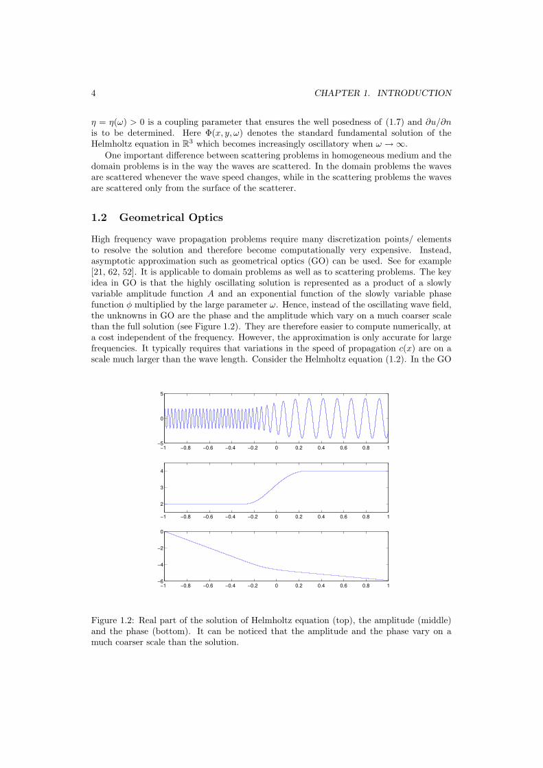
High frequency wave propagation problems require many discretization points/ elementsto resolve the solution and therefore become computationally very expensive. Instead,asymptotic approximation such as geometrical optics (GO) can be used. See for example[21, 62, 52]. It is applicable to domain problems as well as to scattering problems. The keyidea in GO is that the highly oscillating solution is represented as a product of a slowlyvariable amplitude function A and an exponential function of the slowly variable phasefunction φ multiplied by the large parameter ω. Hence, instead of the oscillating wave field,the unknowns in GO are the phase and the amplitude which vary on a much coarser scalethan the full solution (see Figure 1.2). They are therefore easier to compute numerically, ata cost independent of the frequency. However, the approximation is only accurate for largefrequencies. It typically requires that variations in the speed of propagation c(x) are on ascale much larger than the wave length. Consider the Helmholtz equation (1.2). In the GO
−1 −0.8 −0.6 −0.4 −0.2 0 0.2 0.4 0.6 0.8 1−6
−4
−2
0
−1 −0.8 −0.6 −0.4 −0.2 0 0.2 0.4 0.6 0.8 1
2
3
4
−1 −0.8 −0.6 −0.4 −0.2 0 0.2 0.4 0.6 0.8 1−5
0
5
Figure 1.2: Real part of the solution of Helmholtz equation (top), the amplitude (middle)and the phase (bottom). It can be noticed that the amplitude and the phase vary on amuch coarser scale than the solution.

1.2. GEOMETRICAL OPTICS 5
approximation its solution is sought in the form
u(x) = eiωφ(x)∞∑k=0
Ak(x)(iω)−k. (1.8)
Substituting (1.8) in (1.2) and equating to zero the coefficients of the powers of ω yieldsthe Hamilton-Jacobi type eikonal equation for the phase φ
|∇φ| = 1c, (1.9)
and a system of linear transport equations
2∇φ · ∇A0 + ∆φA0 = 0. . . (1.10)2∇φ · ∇An+1 + ∆φAn+1 = ∆An,
for the amplitudes Ak, k = 0, 1, . . . . For large frequencies, Ak, k > 0 in (1.8) can bediscarded, so only the transport equation for A0 remains to be solved in (1.10) and u(x) ≈A0(x)eiωφ(x).
If the eikonal equation (1.9) is solved through the method of characteristics GO can beformulated as a system of ordinary differential equations (ODEs). Let p = ∇φ and definea Hamiltonian
H(x,p) = c(x)|p|.Then, instead of (1.9), we are solving the following system of ODEs
dxdt
= ∇pH(x,p), (1.11)
dpdt
= −∇xH(x,p), (1.12)
where (p(t),x(t)) is a bicharacteristic related to the Hamiltonian H(x,p). The parametriza-tion t corresponds to the phase of the wave φ(x(t)) = φ(x0) + t. There is also a system ofODEs for the amplitude.
Finally, one can introduce a kinetic model of GO. It is based on the interpretation thatrays are trajectories of particles following Hamiltonian dynamics. Let p be the slownessvector defined above and introduce the phase space (t,x,p) such that the evolution ofparticles in this space is given by the system of equations (1.11)–(1.12). Letting f(t,x,p)be a particle density function, it will satisfy the Liouville equation [6, 20]
ft +∇pH · ∇xf −∇xH · ∇pf = 0, (1.13)
where ∇pH and ∇xH are given by (1.11)–(1.12).A disadvantage of asymptotic approximations such as GO is that it cannot capture
some typical wave properties such as diffraction. Diffracted waves are produced when theincident field hits edges, corners or vertexes of the obstacle or when the incident wave hitsthe tangent points of the smooth scatterer (creeping waves). To overcome the problemwith diffracted fields, an asymptotic expansion with correction terms has been proposedby Keller [35] in his geometrical theory of diffraction (GTD). GTD makes up for the GOsolution on the boundary of the scatterer where some terms of this solution vanish. Forexample, GTD expansion of the solution accounts for the phase and the amplitude of thediffracted waves. It does so by means of several laws of diffraction which allow to use thesame principles as in GO to assign a field to each diffracted ray.
Another disadvantage of GO is that it fails when the amplitude A0 is unbounded, atcaustics where waves focus. One way to remedy this is to use Gaussian beams [44, 49, 3].

6 CHAPTER 1. INTRODUCTION
1.3 Numerical Methods
In this section we describe different numerical methods that can be used for the numericalsolution of wave propagation problems. We first consider classical direct numerical methodsand GO based methods. We then discuss more recent developments: methods that have analmost frequency independent computational cost, and so-called time-upscaling methods.The method developed in this thesis is strongly related to these new types of methods.
Direct Numerical Methods
One way to solve partial differential equations numerically is to use finite difference methods,in which the derivatives are approximated by the differences of the neighboring points ona grid [29]. When a PDE is time dependent, one can discretize it first in space (semi-discretization) and then use some ODE solver to advance in time. Different choice ofODE schemes together with a space discretization of a certain order results in differentfinite difference methods. One example is the Crank-Nicolson method that is obtainedwhen the second order space discretization is combined with the trapezoidal rule. Forexplicit methods special attention should be paid to the stability issues, i.e. time step mustbe shorter then the space discretization step (CFL condition). The equation can also bediscretized on a staggered grid which is in some cases computationally advantageous. Onestandard staggered finite difference scheme for wave equations is the Yee scheme introducedby Kane S. Yee in 1966 [63] and further developed by Taflove in the 70s [55, 56].
Finite volume methods are direct methods that are based on the integral form of theequation instead on the differential equation itself [40]. Similarly to the finite differencemethods, the domain is first split into grid cells or finite volumes which do not necessarilyhave to be of the same size. The unknown is then the approximation of the average ofthe solution over each cell. In 1D intervals are used for finite volumes, in 2D one canuse quadrilaterals and approximate the line integrals by the average of the function valueson each side of the line, or triangles and approximate the line integrals along the sidesby the function values at neighboring triangles. In finite volume methods it is easy touse unstructured grids which makes those methods suitable for problems with complexgeometry. However, the extension of finite volume methods to higher order accuracy canbe very complicated.
Finite element methods are based on the variational formulation of the problem which isobtained when the equation is multiplied by test functions and integrated over the domainusing integration by parts [24, 7]. For discrete approximation of the problem, the functionspace S on which the variational formulation is defined is replaced by a finite dimensionalsubspace Sh. The approximation uh of the solution u is expressed as a linear combination ofthe finite number of basis functions φj(x) which are defined to be continuous and nonzeroonly on small subdomains. In that way, time independent problems are transformed intoa sparse system of equations and time dependent problems are transformed into an initialvalue problem for a system of ODEs with sparse matrices. The unknowns are the coefficientsin the linear combination of basis functions. In the time dependent case the vector holdingthe time derivative of the solution is multiplied by a matrix (the mass matrix). The methodtherefore becomes implicit and a system of algebraic equations has to be solved at everytime step which can be computationally costly. There are techniques to avoid this problemby for example approximating the mass matrix by a diagonal matrix (’mass lumping’). Agreat advantage of FEM is that it is mathematically well motivated with rigorous errorestimates. Furthermore, if there is an energy estimate of the original problem, the stabil-ity of the space approximation follows directly. As in finite volume methods unstructured

1.3. NUMERICAL METHODS 7
grids are easy to use and FEM is thus also very well suited for the problems with complexgeometries. It should be noted, however, that adaptivity which can be easily implementedin FEM, only play a limited role in wave propagation problems, since the same wavelengthhas to be resolved everywhere.
In discontinuous Galerkin methods [13], similarly as in FEM, the original problem istransformed into the weak formulation by multiplying the underlying equation by test func-tions and integrating by parts. The difference is that the integration is not done over thewhole domain but over the subintervals which are centered around discretization points sim-ilarly to finite volume methods. The requirement on the continuity of the basis functionsand thus of the solution is now relaxed allowing for discontinuities. The basis functionsare chosen to be nonzero only on one subinterval. Compared to FEM, in a time dependentcase, the problem is transformed into a system of ODEs which can be solved with a fastexplicit difference method, i.e. no algebraic system of equations has to be solved at everytime step. However, the stability of the solution does not follow automatically like in FEM.
In spectral methods [59, 29, 31], the solution is approximated as a linear combination ofsmooth basis functions like Chebyshev or Legendre polynomials or trigonometric functions.The difference from the finite element methods is that the basis functions here are usuallynonzero over the whole domain. Often, spectral methods involve the use of the Fouriertransform. The solution of the problem is first written as its Fourier transform and thensubstituted in the PDE. In that way, a system of ODEs is obtained which then can be solvedwith some ODE solver. Fourier expansion of the solution normally requires the problem tobe periodic. For nonperiodic problems other basis functions are recommended, for exampleChebyshev or Legendre polynomials. Spectral methods have high, exponential, order ofaccuracy, but can be difficult to use in complex geometries.
The direct methods described above can also be applied to the Helmholtz equation. Therelative advantages and disadvantages of the methods are the same in terms of handlingcomplex geometry and boundary conditions. Finite difference, finite element and finitevolume methods lead to sparse systems of equations with the number of unknowns N thatdepends on the frequency, N ∼ ω. For high frequencies, those systems are large anddirect methods like Gaussian elimination become computationally too expensive in higherdimensions. The alternative is to use iterative methods. However, there is a difficultyin this approach, as well. Since the system of equations is indefinite and ill-conditioned,iterative methods have slow convergence rate. The convergence rate can be improved bypreconditioning but finding a good preconditioner for Helmholtz equation is still a challenge[25]. The indefiniteness makes it difficult to use multigrid and the conjugate gradientmethod. Typically Krylov subspace methods, like GMRES or Bi-CGSTAB are used instead.Preconditioners can for instance be based on incomplete LU-factorization [43] or on fasttransform methods [47, 39, 27, 18]. More recently preconditioners based on a complexshifted Helmholtz operator has been introduced [26].
For scattering problems one needs to solve an integral equation of type (1.7), see forexample [14, 36]. Let us consider a simplified version of (1.7) in 1D∫ b
a
Φ(x, y, ω)u(y)ds(y) = f(x), x ∈ [a, b]. (1.14)
One way to solve (1.14) numerically is to use the collocation method. The idea in thismethod is to approximate u(x) by
u(x) =N∑j=1
cjϕj(x),
8 CHAPTER 1. INTRODUCTION
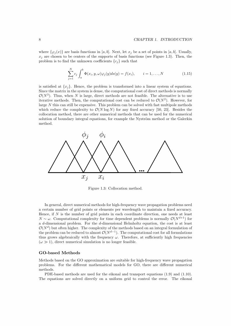
where ϕj(x) are basis functions in [a, b]. Next, let xj be a set of points in [a, b]. Usually,xj are chosen to be centers of the supports of basis functions (see Figure 1.3). Then, theproblem is to find the unknown coefficients cj such that
N∑j=1
cj
∫ b
a
Φ(xi, y, ω)ϕj(y)ds(y) = f(xi), i = 1, . . . , N (1.15)
is satisfied at xj. Hence, the problem is transformed into a linear system of equations.Since the matrix in the system is dense, the computational cost of direct methods is normallyO(N3). Thus, when N is large, direct methods are not feasible. The alternative is to useiterative methods. Then, the computational cost can be reduced to O(N2). However, forlarge N this can still be expensive. This problem can be solved with fast multipole methodswhich reduce the complexity to O(N logN) for any fixed accuracy [50, 23]. Besides thecollocation method, there are other numerical methods that can be used for the numericalsolution of boundary integral equations, for example the Nystrom method or the Galerkinmethod.
Figure 1.3: Collocation method.
In general, direct numerical methods for high-frequency wave propagation problems needa certain number of grid points or elements per wavelength to maintain a fixed accuracy.Hence, if N is the number of grid points in each coordinate direction, one needs at leastN ∼ ω. Computational complexity for time dependent problems is normally O(Nd+1) fora d-dimensional problem. For the d-dimensional Helmholtz equation, the cost is at leastO(Nd) but often higher. The complexity of the methods based on an integral formulation ofthe problem can be reduced to almostO(Nd−1). The computational cost for all formulationsthus grows algebraically with the frequency ω. Therefore, at sufficiently high frequencies(ω 1), direct numerical simulation is no longer feasible.
GO-based Methods
Methods based on the GO approximation are suitable for high-frequency wave propagationproblems. For the different mathematical models for GO, there are different numericalmethods.
PDE-based methods are used for the eikonal and transport equations (1.9) and (1.10).The equations are solved directly on a uniform grid to control the error. The eikonal
1.3. NUMERICAL METHODS 9
equation is a Hamilton-Jacobi type equation and it has a unique viscosity solution whichcan be computed numerically by finite difference methods for example. Some of them areupwind-based methods like the fast marching method [53, 61] and the fast sweeping method[60]. For time dependent eikonal equations one can use high-resolution methods of ENOand WENO type [46]. However, at points where the correct solution is multivalued theviscosity solution is not enough because the eikonal and the transport equations describeonly one unique wave at a time. Therefore, some other numerical techniques must be used.Some examples are the big ray tracing method, the slowness matching method and thedomain decomposition based on detecting kinks in the viscosity solution. In all methods,the solution is obtained by solving several eikonal equations.
Ray tracing methods [12, 33, 37, 57] are used to solve the ray equations (1.11)–(1.12).That system can be augmented with another system of ODEs for the amplitude. TheODEs are solved with standard numerical methods for example second or fourth orderRunge-Kutta methods. The phase and the amplitude are calculated along the rays andthe interpolation must be used to obtain the solution in points other than the grid points.However in regions with diverging or crossing rays this method is not efficient.
Methods based on the kinetic formulation of GO are phase space methods. The Liouvilleequation (1.13) has a large number of independent variables and therefore a lot of unknownshas to be used in the numerical methods which can be computationally ineffective. Toovercome this problem one can use wave-front methods and moment-based methods. Inwave-front methods a wave front is evolved following the kinetic formulation. Some ofthe wave front methods are the level set method [45] and the segment projection method[22, 58]. In moment-based methods a kinetic transport equation set in a high-dimensionalphase space (t,x,p) is approximated by a finite system of moment equations in the reducedspace (t,x). In that way, the number of unknowns is decreased. For more details, see [6, 51].
Methods with Weakly Frequency Dependent Cost
The situation described above can be summarized as follows: For direct methods the com-putational cost grows with frequency for fixed accuracy, while for GO methods the accuracygrows with frequency for fixed computational cost. Unfortunately, the frequency range andaccuracy requirement of many realistic problems often fall in between what is tractable witheither of these approaches.
Recently a new class of algorithms have been proposed that combine the cost advantageof GO methods with the accuracy advantage of direct methods. They are thus characterizedby a computational cost that grows slowly with the frequency, while at the same time beingaccurate also for moderately high frequencies. It should be noted that one needs at leastO(ω) points to resolve the solution. If that many points are used, then the computationalcost is, of course, at least O(ω). In these methods, however, one does not resolve thesolution, but computes instead GO like solutions. Therefore, one can only expect to get thefull solution in O(1) points.
The main interest of the new methods have been for scattering problems [8, 38, 16, 1, 32].Those methods are based on the integral formulation of the Helmholtz equation (1.7). Thekey step is to write the surface potentials as a slowly varying function multiplied by a fastphase variation. Instead of approximating the unknown function v := ∂u/∂n directly, thefollowing ansatz is used
v(x, ω) ≈ ωeiωφ(x)V (x), x ∈ ∂Ω. (1.16)
The basic idea is that, using asymptotic analysis, the phase function φ can be determined insuch a way that V (x) is much less oscillatory than the original unknown function v. More

10 CHAPTER 1. INTRODUCTION
precisely, φ(x) is taken as the phase of the geometrical optics approximation. For instance,when uinc is a plane wave in direction d, then φ = x · d. Hence, the ansatz becomes
v(x, ω) = ωeiωx·dV (x, ω), (1.17)
where V now varies slowly with ω. Each side of (1.7) is then multiplied by e−iωx·d to obtain
12V +DV − iηSV = i(ωd · n− η), (1.18)
where the operators S and D are defined as follows
SV (x) =∫∂Ω
Φ(x, y, ω)eiω(y−x)·dV (y)dy, (1.19)
DV (x) =∫∂Ω
∂Φ(x, y, ω)∂n(x)
eiω(y−x)·dV (y)dy. (1.20)
Thus, the problem becomes to find the amplitude V (x, ω) by solving the integral equation(1.18). The amplitude varies slowly away from the shadow boundaries and can be rep-resented by a fixed set of grid points, i.e. independently of the frequency. The integralequation can be solved for example with the collocation method. In this method one needsto compute integrals of the type given in (1.15). Although the amplitude is a slowly vary-ing function, the integrals cannot be computed independently of the frequency by directnumerical methods since their kernels are oscillatory (c.f. (1.19)–(1.20)). To overcome thisproblem an extension of the method of stationary phase has been suggested [8]. Since thevalues of the integrands and their derivatives in critical points make the only significantcontributions to the oscillating integrals, an integration procedure based on localizationaround those points was introduced. Since the amplitude near shadow boundaries is vary-ing rapidly, those regions are treated with special consideration. However the method worksmainly for problems with convex scatterers. For more information about these methods see[11]. The extension of the method to non-convex scatterers is proposed in [9, 17].
Rigorous proofs of the low cost of these methods is difficult and requires detailed resultson the asymptotic behaviour of the exact solution near shadow boundaries. An example of aresult, due to Dominguez, Graham and Smyshlyaev [16], concerns convex smooth scatterersin 2D. They show that for a Galerkin discretization with N unknowns where the integralscorresponding to (1.19), (1.20) are computed exactly, the relative error in V (y) can beestimated as
rel. err ∼ kα((
k1/9
N
)6
+ e−Ck1/3
),
where α is a small exponent less than one. Hence, if N is slightly larger than k1/9 the erroris controlled.
For full domain problems much less has been done. In some sense this is more difficultthan the scattering problem in a homogeneous medium because the waves are reflectedat all points where the wave speed changes, not only at the surface of a scatterer. Oneattempt at lowering the computational cost along the lines above has been to use ”planewave basis functions” in finite element methods [48, 28, 10]. The method can be seen asa Discontinuous Galerkin method with a particular choice of basis functions. However,except in simple cases these methods do not reduce the complexity more than by a constantfactor. The method proposed by Giladi and Keller [28] is a hybrid numerical method forthe Helmholtz equation in which the finite element method is combined with GO. The idea
1.3. NUMERICAL METHODS 11
is to determine the phase factor which corresponds to the plane wave direction a prioriby solving the eikonal equation for the phase using ray tracing and then to determine theamplitude by a finite element method choosing asymptotically derived basis functions whichincorporate the phase factor.
A tailored finite-point method for the numerical simulation of the Helmholtz equationwith high frequency in heterogeneous medium has been recently proposed by Han andHuang in [30]. They suggest to approximate the wave speed function c(x) by a piecewiseconstant function and then solve the equation on every subdomain exactly. The speedfunction is assumed to be smooth and monotone in each interval.
Time Upscaling Methods
Time upscaling methods have been proposed to overcome the problem with computationalcomplexity of direct simulation of time dependent wave propagation. The aim is to reducethe extra cost incurred by the time–stepping. There is an interesting connection betweenthese methods and methods with frequency independent cost, which will be described atthe end of this section.
Let us now consider a d–dimensional problem and suppose N discretization points inevery space direction and M discretization points in time. For explicit methods, due to thestability (CFL) and accuracy requirements it is necessary to have M ∼ Nr where r = 1 forhyperbolic problems and r = 2 for parabolic problems. Then, the computational cost fora time interval of O(1) is O(Nd+r). With time upscaling the computational cost can bereduced to O(Nd logN) or even to O(Nd) while maintaining the same accuracy.
For the advection and parabolic equations with spatially varying coefficients, time up-scaling methods are proposed in [19]. The authors suggest to use the fast transform wavelettogether with truncation. Consider the following evolution equation
∂tu+ L(x, ∂x)u = 0, x ∈ Ω ⊂ Rd, t > 0,u(x, 0) = u0(x),
where L is a differential operator. After discretization, collecting the unknowns in a vectoru ∈ RNd
, the equation becomes
un+1 = Aun, (1.21)
u0 = u0,
where A is a Nd × Nd matrix approximating the operator ∂t + L. The computationalcomplexity is of order O(Nd+r). Clearly, (1.21) is equivalent to
un = Anu0. (1.22)
Then, repeated squaring of A can be used to compute the solution of (1.22) in log2M stepsfor M = 2m, where m is an integer, i.e. one can compute A,A2, A4, . . . , A2m
in m = log2Msteps. Since the matrix A is sparse, the cost of squaring is O(Nd). However, the latersquarings involve almost dense matrices and the computational cost is then O(N3d). Thetotal cost becomes O(N3d logM) which is more expensive than to solve (1.21) directly.Instead, Engquist, Osher and Zhong in [19] suggest a wavelet representation of A which candecrease the computational complexity of the repeated squaring algorithm. More precisely,

12 CHAPTER 1. INTRODUCTION
the solution of (1.22) can be computed in m = log2M steps in the following way
B := SAS−1,
B := TRUNC(B2, ε) (iteratem steps) (1.23)
un := S−1BSu0.
The matrix S corresponds to a fast wavelet transform and the truncation operator TRUNCsets all elements of A that are less than ε to 0. It is obvious that the algorithm (1.23) isequivalent to (1.22) for ε = 0 and it was shown in [19] that there exist a small enough ε suchthat the result of the algorithm (1.23) is close to (1.22). Through truncation the algebraicproblem with dense matrices is transformed to a problem with sparse matrices. The authorsalso showed that the cost to compute the 1D hyperbolic equation can be reduced fromO(N2)to O(N log3N) for a fixed accuracy. Furthermore, for d–dimensional parabolic problemsthe computational complexity can be reduced from O(Nd+2) to O(Nd(logN)3).
A similar technique is proposed in [15] by Demanet and Ying. They consider the 2Dwave equation
utt − c2(x)∆u = 0, x ∈ [0, 1]2
u(x, 0) = u0, ut(x, 0) = u1,
with periodic boundary conditions. They assume c(x) ∈ C∞ to be positive and boundedaway from zero and propose to transform the wave equation into a first order system ofequations,
vt = Av, v(t = 0) = v0,
where v = (ut, ux) and A is a 2-by-2 matrix of operators. The system is then solved up totime t = T using wave atoms, which provide a sparse representation of the matrix, combinedwith repeated squaring and truncation as above. On a N by N grid the computational costis reduced from O(N3 logN) of pseudo-spectral methods to O(N2+δ) for arbitrarily smallδ of naive version of the wave atom method. For the final algorithm they proved rigorouslythat the computational cost is between O(N2.25) and O(N3) depending on the initial dataand the structure of c(x). The key of the proof is to show that the solution operator eAt
remains almost sparse for all t in the wave atom basis.Another fast time upscaling method for the one-dimensional wave equation is proposed
by Stolk [54]. The idea here is first to rewrite the wave equation as a system of one–waywave equations, then transform them into wavelet bases and solve using multiscale steppingwhich means that the fine spatial scales are solved with longer time steps and the coarsespatial scales are solved with the shorter time steps. The computational cost is only O(N)for fixed accuracy.
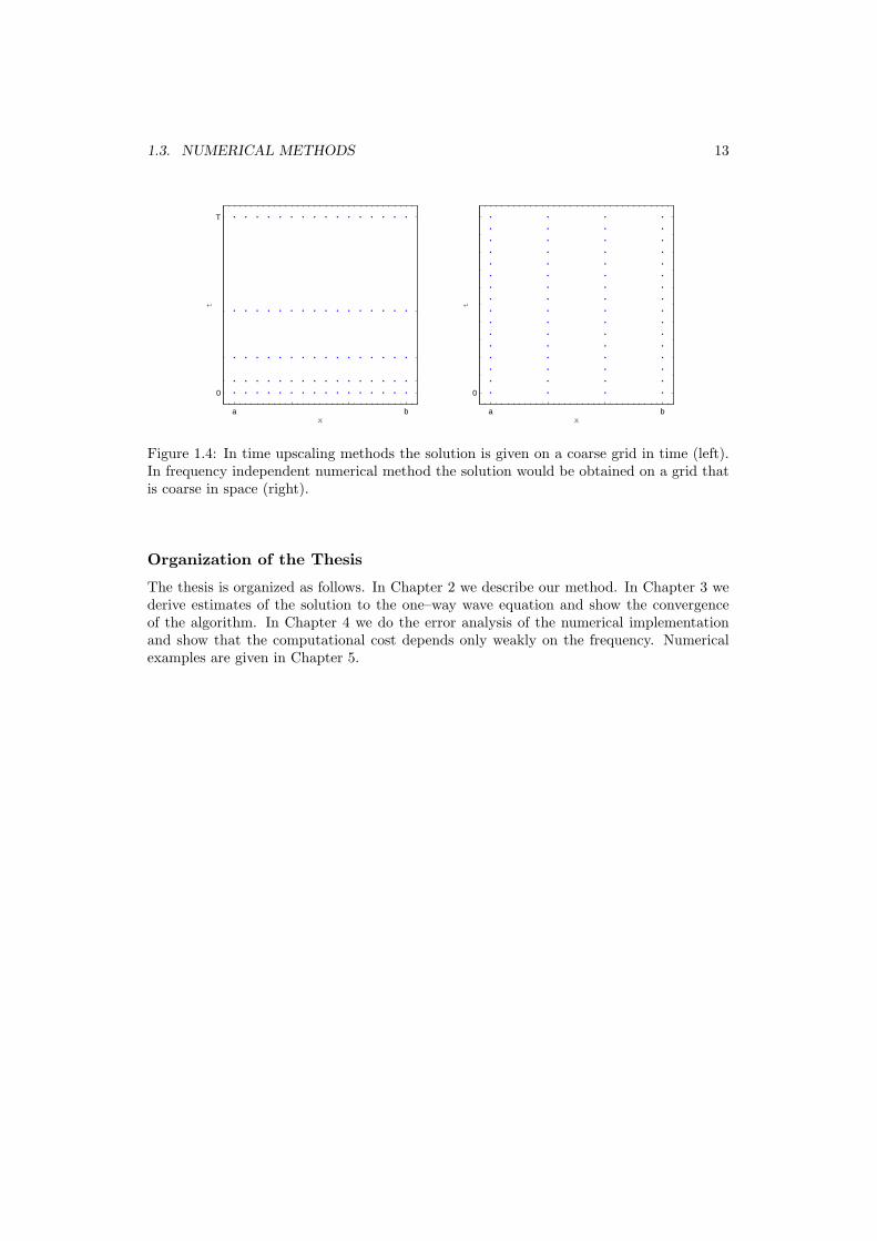
Hence, it can be noted that when the wave equation is solved with the time upscalingmethods with repeated squaring, the solution is given on a grid that is coarse in timeand dense in space direction. One can also solve the wave equation by solving Helmholtzequations for each frequency component. This is like taking a Fourier/Laplace transform intime. A space discretization with N points then corresponds to N Helmholtz equations forN frequency components. If the Helmholtz equation is solved with a frequency independentmethod, then the total cost is O(N), but the solution is obtained only in O(1) points. Afteran inverse FFT for each point at a cost of O(N logN) the solution of the wave equation isobtained on a dense grid in time but coarse in space at a total cost O(N logN), i.e. thesame as in time upscaling, see Figure 1.4.
1.3. NUMERICAL METHODS 13
a b
0
T
x
t
a b
0
x
tFigure 1.4: In time upscaling methods the solution is given on a coarse grid in time (left).In frequency independent numerical method the solution would be obtained on a grid thatis coarse in space (right).
Organization of the Thesis
The thesis is organized as follows. In Chapter 2 we describe our method. In Chapter 3 wederive estimates of the solution to the one–way wave equation and show the convergenceof the algorithm. In Chapter 4 we do the error analysis of the numerical implementationand show that the computational cost depends only weakly on the frequency. Numericalexamples are given in Chapter 5.


Chapter 2
A Fast Method for HelmholtzEquation
We focus on the high frequency wave propagation problem in a bounded domain with avarying wave–speed function. The problem is described by the Helmholtz equation aug-mented with non-reflecting boundary conditions that also incorporate an incoming wave.The computational complexity of direct numerical methods applied to this problem growsalgebraically with the frequency ω. The computational cost is at least O(ωd) for a d-dimensional problem. Therefore, direct numerical simulations become inapplicable for suf-ficiently high frequencies and some other methods have to be used. We propose a fastmethod for solving the Helmholtz equation based on wave–splitting. The Helmholtz equa-tion is split into one–way wave equations (backward and forward), which are then solvedwith appropriate boundary conditions and approximate forcing functions. In a domainwhere the forcing function is equal to zero GO is used and some standard p-th order nu-merical method otherwise. The result is an approximation of a type of Bremmer series [5].In this chapter we present the model and describe our method. In later chapters we willshow that the algorithm is convergent and that for fixed accuracy, the computational costis O(ω1/p) for a p-th order numerical method.
We consider mainly a model problem in one dimension, but we will also describe howthe algorithm can be extended to higher dimensions. Although there are already someinteresting applications in one dimension, e.g. inverse problems for transmission lines [41],most practical problems are of course in higher dimensions. Our focus in this thesis ison the analysis of the method and to show rigorous error and cost estimates. For higherdimensions, however, this is a much harder problem and we will restrict the analysis to theone-dimensional case.
2.1 Derivation of the Method in One Dimension
Consider the 1D Helmholtz equation
uxx +ω2
c(x)2u = ωf, x ∈ [−L,L], (2.1)
15

16 CHAPTER 2. A FAST METHOD FOR HELMHOLTZ EQUATION
where ω is the frequency and c(x) is the wave–speed function such that supp(cx) ⊂ (−L,L).We augment the equation (2.1) with the following boundary conditions
ux(−L)− iωu(−L) = −2iωA, (2.2)ux(L) + iωu(L) = 0, (2.3)
where A is the amplitude of the incoming wave. At high frequencies GO is a good approx-imation of the solution. We want to find a way to correct for the errors it makes at lowerfrequencies. A natural idea would be to use the system of WKB equations (1.10). However(1.8) does not converge, even in simple settings. It is only an asymptotic series. Moreprecisely, a problem with (1.10) is that it only describes waves traveling in one direction. Inreality, waves are reflected whenever cx 6= 0. Hence, to incorporate two directions we makethe ansatz
iωv + c(x)vx −12cx(x)v = F, (2.4)
iωw − c(x)wx +12cx(x)w = F. (2.5)
This describes wave propagation in the right-going (v) and left-going (w) direction. More-over, if z = v + w, then it satisfies the following equation (see Lemma 1)
c2zxx + ω2z = −2iωF + α(x)z,
whereα(x) =
12ccxx −
14c2x. (2.6)
Thus, if F = α(x)z/2iω, then z is the solution of the Helmholtz equation (2.1) with f = 0.We now make an expansion of v and w in powers of ω,
v =∑n
rnω−n, w =
∑n
snω−n. (2.7)
Then, (2.4) and (2.5) become∑n
(iωrn + c(x)∂xrn −
12cx(x)rn −
α(x)2i
(rn−1 + sn−1))ω−n = 0,
∑n
(iωrn − c(x)∂xsn +
12cx(x)sn −
α(x)2i
(rn−1 + sn−1))ω−n = 0.
Defining vn = rnω−n and wn = snω
−n and equating terms with the same powers in ω tozero, we obtain the methods below. In contrast to (1.8) the series (2.7) converge quicklyfor large ω.
Method 1
Let
iωvn + c(x)∂xvn −12cx(x)vn = − 1
2iωfn(x) (2.8)
iωwn − c(x)∂xwn +12cx(x)wn = − 1
2iωfn(x) (2.9)

2.1. DERIVATION OF THE METHOD IN ONE DIMENSION 17
for x ∈ [−L,L] and n ≥ 0, with the initial conditions:
vn(−L) =A, n = 00, n > 0 (2.10)
andwn(L) = 0, ∀n. (2.11)
The right hand side in (2.8) and (2.9) is defined by the following expression
f0(x) = ωf(x), (2.12)fn+1(x) = −α(x)(vn(x) + wn(x)). (2.13)
Assume we are solving equations (2.8) and (2.9) for n = 0, 1, 2, . . . ,m with the given initialconditions (2.10) and (2.11) and the source function fn that is defined by (2.12)–(2.13).Then, it can be shown that the solution u(x) of the Helmholtz equation (2.1) can be ap-proximated by the following sum
u(x) ≈ zm =m∑k=0
(vk(x) + wk(x)). (2.14)
Remark 1. This is similar to Bremmer series [5], where
iωvn(x) + c(x)∂xvn(x)− cx(x)2
vn(x) = −cx2wn−1(x),
iωwn(x)− c(x)∂xwn(x) +cx(x)
2wn(x) =
cx2vn−1(x),
with no ω−1 in the right hand side. The convergence is more subtle but has been shown in[2, 34, 4, 42]. We prefer (2.8)–(2.9) as it clearly separates waves of different size in termsof ω−1, which leads to a simpler analysis.
Thus, we can solve equations (2.8) and (2.9) with some p-th order ODE numerical methodm ≥ 0 times and approximate the solution of (2.1) by (2.14). However, the computationalcomplexity still grows algebraically with the frequency ω.
Method 2
Now, note that (2.8) and (2.9) can be simplified when fn = 0. Then, using the ansatz
vn = Aeiωφ
in (2.8) we obtain equations for A and φ,
∂xφ =1c(x)
, ∂xA =cx(x)2c(x)
A(x). (2.15)
This is in fact GO and can be solved independently of the frequency. Similar equations canbe obtained when the ansatz is used in (2.9). Thus, the computational cost estimate canbe improved by approximating the forcing functions. We can do the following:
Replace fn by fn with
fn(x) =
0, |fn(x)| < Tolnfn(x), otherwise
(2.16)

18 CHAPTER 2. A FAST METHOD FOR HELMHOLTZ EQUATION
where
Toln =ωTol
2n+1L(2.17)
for some tolerance Tol. More precisely, let f0 = ωf and define
iωvn + c(x)∂xvn −12cx(x)vn = − 1
2iωfn(x) (2.18)
iωwn − c(x)∂xwn +12cx(x)wn = − 1
2iωfn(x) (2.19)
with initial data
vn(−L) =A, n = 00, n > 0 (2.20)
and
wn(L) = 0, ∀n. (2.21)
Moreover,
fn+1(x) = −α(x)(vn(x) + wn(x)). (2.22)
Again it can be shown that the solution u(x) of the Helmholtz equation (2.1) can be ap-proximated by
u(x) ≈ zm =m∑k=0
(vk(x) + wk(x)). (2.23)
Thus, equations (2.18)–(2.19) can be solved independently of the frequency in a domainwhere fn = 0. In a domain where fn 6= 0 a direct ODE numerical method can be used.The solution of (2.1) is then approximated by (2.23).
Hence, the algorithm for computing the solution of (2.1)–(2.3) is as follows: Choosesome tolerance Tol and, for n = 0, 1, 2, . . . , do the following
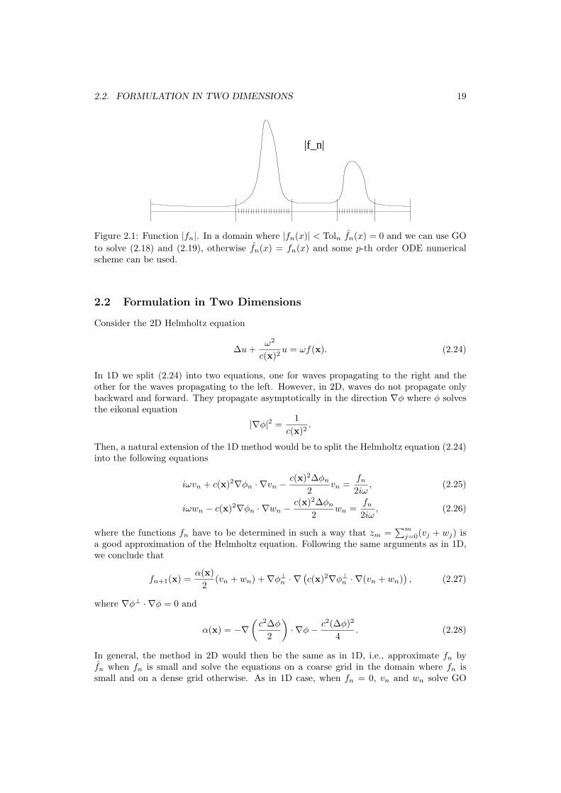
1. Replace the function fn by fn defined by (2.16). If fn ≡ 0 stop, else
2. Compute vn and wn from (2.18) and (2.19). In a domain where fn 6= 0 use a di-rect p-th order numerical method with stepsize ∆xf = Tol1/p/ω1+1/p, otherwise usegeometrical optics with stepsize ∆xc = ω∆xf , Figure 2.1,
3. Compute un = vn + wn and add un to un−1. Note that in a Runge-Kutta scheme thefunction fn may need to be evaluated in between the grid points. To obtain thosevalues of fn, we use p-th order interpolation.
4. Compute fn+1 from vn and wn, go to 1.
The solution of (2.1)–(2.3) is approximated by∑k uk.
These methods converge rapidly for large ω as we prove in the following chapters. Wewill also show that the computational cost is proportional to ω1/p for a fixed tolerance,where p is the order of the numerical scheme.
2.2. FORMULATION IN TWO DIMENSIONS 19
|f_n|
Figure 2.1: Function |fn|. In a domain where |fn(x)| < Toln fn(x) = 0 and we can use GOto solve (2.18) and (2.19), otherwise fn(x) = fn(x) and some p-th order ODE numericalscheme can be used.
2.2 Formulation in Two Dimensions
Consider the 2D Helmholtz equation
∆u+ω2
c(x)2u = ωf(x). (2.24)
In 1D we split (2.24) into two equations, one for waves propagating to the right and theother for the waves propagating to the left. However, in 2D, waves do not propagate onlybackward and forward. They propagate asymptotically in the direction ∇φ where φ solvesthe eikonal equation
|∇φ|2 =1
c(x)2.
Then, a natural extension of the 1D method would be to split the Helmholtz equation (2.24)into the following equations
iωvn + c(x)2∇φn · ∇vn −c(x)2∆φn
2vn =
fn2iω
, (2.25)
iωwn − c(x)2∇φn · ∇wn −c(x)2∆φn
2wn =
fn2iω
, (2.26)
where the functions fn have to be determined in such a way that zm =∑mj=0(vj + wj) is
a good approximation of the Helmholtz equation. Following the same arguments as in 1D,we conclude that
fn+1(x) =α(x)
2(vn + wn) +∇φ⊥n · ∇
(c(x)2∇φ⊥n · ∇(vn + wn)
), (2.27)
where ∇φ⊥ · ∇φ = 0 and
α(x) = −∇(c2∆φ
2
)· ∇φ− c2(∆φ)2
4. (2.28)
In general, the method in 2D would then be the same as in 1D, i.e., approximate fn byfn when fn is small and solve the equations on a coarse grid in the domain where fn issmall and on a dense grid otherwise. As in 1D case, when fn = 0, vn and wn solve GO

20 CHAPTER 2. A FAST METHOD FOR HELMHOLTZ EQUATION
equations. Note that C = constant does not imply that α = 0 as in one dimension. Hence,GO is not exact when a wave front is curved. Moreover, the ∇(vn + wn) term in (2.27)may now possibly be large. However, when vn is a wave of the form vn = Aeiωφn , then∇φ⊥n · ∇vn = ∇φ⊥n · ∇Aeiωφn = O(1). There is a number of additional difficulties:
• Caustics appear. This implies that ∇φ may not exist everywhere. That means thatone has to resolve everything also in an area around caustics. (The size of this is stillsmall though.)
• Multiple crossing waves. One will need a formula for computing φn+1 from vn, wnand φn.
• Analysis is much harder. There are no L∞ estimates with ω-independent constantsavailable.
Chapter 3
Analysis
In this chapter we analyze the method when (2.18) and (2.19) are solved exactly. We willfirst derive estimates of the solution of the equations (2.8) and (2.9) and its derivatives. Wethen show that zm in (2.23) converges to the solution of (2.1)–(2.3). Next, we give an errorestimate in terms of n and Tol. As a side effect we obtain a L∞ estimate of the solutionof the Helmholtz equation in 1D. We also show that the size of the domain where a directmethod, which resolves the wavelength, is used is proportional to O(ω1/p). Hence, we provethe following
Theorem 1. Assume ω > 1, c(x) ∈ C2[−L,L], and
2β|α|L1
ω≤ δ0 < 1, β =
12
√cmaxc3min
. (3.1)
If u is the solution of (2.1)–(2.3), then
|u− zm|∞ ≤ C((|A|+ |f |L1)δm+1
0 + Tol). (3.2)
Moreover,
measfn 6= 0 = meas|fn| ≥ Toln ≤C
ω, (3.3)
and|u|∞ ≤ C(|A|+ |f |L1). (3.4)
The constants in (3.2)–(3.4) do not depend on ω.
Remark 2. If Tol = 0, (3.2) shows the convergence of method 1. From (3.3) it follows thatthe computational cost of our method will not grow fast with ω. More precisely,
cost ∼ 1∆xc
+measfn 6= 0
∆xf= O(ω1/p).
3.1 Utility Results
In order to prove Theorem 1, we begin by deriving some useful utility results. Consider thefollowing initial value problem
d
dxy = iωa(x, ω)y + b(x, ω), x0 ≤ x ≤ x1 (3.5)
y(x0) = y0. (3.6)
21
22 CHAPTER 3. ANALYSIS
where a(x, ω) and b(x, ω) are given functions that depend on the frequency ω. Before wecontinue, note that equations (2.8) and (2.9) can be rewritten in the form of (3.5). If wedefine
a(x, ω) = − 1c(x)
− i cx(x)2c(x)ω
(3.7)
b(x, ω) = − 12iωc(x)
fn(x), (3.8)
(2.8) and (2.9) become
dvndx
= iωa(x, ω)vn + b(x, ω) (3.9)
dwndx
= iωa(x, ω)wn − b(x, ω). (3.10)
Theorem 2. Consider (3.5)–(3.6). Suppose
• ω > 1,
• a(x, ω), b(x, ω) ∈ Ck−1([x0, x1]), for each ω > 1
• supx0≤x≤x1|∂pxa(x, ω)| < Cp, ∀ω, 0 ≤ p ≤ k − 1, where Cp is some constant indepen-
dent of ω,
• −ω · Im(a(x, ω)) ≤ a0 for some constant a0 independent of ω.
LetC0 = sup
x0≤t,x≤x1
∣∣∣e−ω R xtIm(a(s,ω))ds
∣∣∣ . (3.11)
If y(x) is a solution of (3.5)–(3.6), then
|y|∞ ≤ C0 (|y0|+ |b|L1) , (3.12)
∣∣∂kxy∣∣∞ ≤ Ck(ωk|y0|+
k∑i=1
ωi−1|∂k−ix b(x, ω)|∞ + ωk|b|L1
), k ≥ 1, (3.13)
where Ck, k ≥ 0, are some constants that do not depend on ω or b(x, ω).
Proof. Let us first prove (3.12). The exact solution of (3.5)–(3.6) is given by
y(x) = y0eiωR x
x0a(s,ω)ds +
∫ x
x0
b(t, ω)eiωR x
ta(s,ω)dsdt. (3.14)
Then
|y|∞ ≤ supx0≤x≤x1
∣∣∣eiω R xx0a(s,ω)ds
∣∣∣ |y0|+ supx0≤x≤x1
∣∣∣∣∫ x
x0
b(t, ω)eiωR x
ta(s,ω)dsdt
∣∣∣∣≤ supx0≤x≤x1
∣∣∣eiω R xx0a(s,ω)ds
∣∣∣ |y0|+ supx0≤t,x≤x1
∣∣∣eiω R xta(s,ω)ds
∣∣∣ |b|L1
≤ supx0≤x≤x1
∣∣∣e−ω R xx0Im(a(s,ω))ds
∣∣∣ |y0|+ supx0≤t,x≤x1
∣∣∣e−ω R xtIm(a(s,ω))ds
∣∣∣ |b|L1
≤ C0 (|y0|+ |b|L1) ,
3.2. ESTIMATES OF ONE-WAY SOLUTIONS 23
where C0 is defined by (3.11). Thus, (3.12) is proved.To prove (3.13) we use mathematical induction. From (3.5), it follows
|∂xy|∞ ≤ ω|a|∞|y|∞ + |b|∞≤ C (ω|y|∞ + |b|∞)≤ C1 (ω|y0|+ |b|∞ + ω|b|L1) . (3.15)
Hence, (3.13) is true for k = 1. Next, assume that (3.13) is true for k ≤ n for some n ≥ 1and show that it is true for k = n + 1. Since (n + 1)st derivative of y(x) is given by thefollowing formula
∂n+1x y = iω
n∑j=0
Cjn∂n−jx a · ∂jxy + ∂nx b, Cjn =
n(n− 1)...(n− k + 1)k!
,
and (3.13) is true for k ≤ n, then
∣∣∂n+1x y
∣∣∞ ≤ ω
n∑j=0
Cjn∣∣∂n−jx a
∣∣∞
∣∣∂jxy∣∣∞ + |∂nx b|∞
≤ Cωn∑j=1
Cjn∣∣∂n−jx a
∣∣∞
(ωj |y0|+
j∑i=1
ωi−1|∂j−ix b|∞ + ωj |b|L1
)+ |∂nx b|∞
≤ Cω
n∑j=1
ωj |y0|+n∑j=1
j∑i=1
ωi−1|∂j−ix b|∞ +n∑j=1
ωj |b|L1
+ |∂nx b|∞ . (3.16)
Before we continue, let us estimate
n∑j=1
j∑i=1
ωi−1|∂j−ix b|∞ =n∑i=1
|∂n−ix b|∞i−1∑j=0
ωj
≤ Cn∑i=1
ωi−1|∂n−ix b|∞.
Hence, (3.16) becomes
∣∣∂n+1x y
∣∣∞ ≤ Cn+1
(ωn+1|y0|+
n∑i=1
ωi|∂n−ix b|∞ + ωn+1|b|L1 + |∂nx b|∞
)
= Cn+1
(ωn+1|y0|+
n+1∑i=1
ωi−1|∂n+1−ix b|∞ + ωn+1|b|L1
).
This proves the theorem.
3.2 Estimates of One-Way Solutions
Here we derive the bounds on the solution and its derivatives of the equations (2.8) and(2.9). We also show that |vn|∞ → 0 (|wn|∞ → 0), |∂pxvn|∞ → 0 (|∂pxwn|∞ → 0) and|fn|∞ → 0 under some assumption. Let us prove the following
24 CHAPTER 3. ANALYSIS
Theorem 3. Let vn(x) be a solution of (2.8) and let p ≥ 0. Assume c(x) ∈ Cp[−L,L] andω > 1. Then
|∂pxvn|∞ ≤ Cωp(|A|+ |f |L1)(β
ω|α|L1
)n, n ≥ 0. (3.17)
and
|fn|L1 ≤ C|α|L1(|A|+ |f |L1)(β
ω|α|L1
)n−1
, n ≥ 1. (3.18)
Estimate (3.17) is valid for |wn|∞ and |∂pxw|∞.
Proof. Since the solution of (2.8) is given by (3.14), where a(x, ω) and b(x, ω) are definedby (4.1) and (4.2), we can use Theorem 2. Let us first verify that a(x, ω) and b(x, ω) satisfythe assumptions. The assumptions 1, 2 and 3 from Theorem 2 follow directly from theassumptions in this theorem. Let us check the assumption 4. Since
−ω · Im(a(x, ω)) =cx(x)2c(x)
and c(x) ∈ Cp[−L,L], then there exist some constant a0 such that the assumption 4 issatisfied. Now, we can prove Theorem 3. We begin with the estimate (3.17) for p = 0. Letus first calculate C0 and |b|L1 .
C0 = supx0≤t,x≤x1
∣∣∣e−ω R xtIm(a(s,ω))ds
∣∣∣= supx0≤t,x≤x1
∣∣∣eω R xt
cs2c(s)ω
ds∣∣∣
= supx0≤t,x≤x1
∣∣∣∣eR xtd“
ln(√c(s))
”ds
∣∣∣∣= supx0≤t,x≤x1
√c(x)√c(t)
≤ 2βcmin,
where β is the constant defined by (3.1). For |b|L1 , we can estimate
|b|L1 =∣∣∣∣− 1
2iωc(x)fn(x)
∣∣∣∣L1
≤ 12ωcmin
|fn|L1 .
Hence,
|vn|∞ ≤ 2βcmin
(|vn(x0)|+ 1
2ωcmin|fn|L1
)≤ |vn(x0)|C +
β
ω|fn|L1 .
When n = 0, v0(x0) = A and f0(x) = ωf(x). Hence,
|v0|∞ ≤ C|A|+ β|f |L1 ≤ C(|A|+ |f |L1). (3.19)
For n ≥ 1, vn(x0) = 0, so
|vn|∞ ≤β
ω|fn|L1 . (3.20)

3.2. ESTIMATES OF ONE-WAY SOLUTIONS 25
Using (2.13), we can estimate |fn|L1 , i.e., for n = 1
|f1|L1 ≤∫
R|α(x)| |v0(x) + w0(x)| dx
(3.19)
≤ C (|A|+ |f |L1)∫
R|α(x)|dx
≤ |α|L1C (|A|+ |f |L1)
and we use mathematical induction to prove that (3.18) is also valid for n ≥ 2. So, assumethat (3.18) is true for n = k and show that it is true for n = k + 1,
|fk+1|L1 ≤∫
R
|α(x)| |vk(x) + wk(x)| dx
(3.20)
≤ β
ω|fk|L1 |α|L1
(3.18),n=k
≤ Cβ
ω|α|L1(|A|+ |f |L1)|α|L1
(β
ω|α|L1
)k−1
= C|α|L1(|A|+ |f |L1)(β
ω|α|L1
)k.
Hence, (3.18) is proved and from (3.20) and (3.18) it follows that
|vn|∞ ≤ C (|A|+ |f |L1)(β
ω|α|L1
)n, ∀n.
To prove (3.17) for p ≥ 1, we again use mathematical induction and Theorem 2. Thus,since we have already proved (3.17) for p = 0, we assume that (3.17) is true for derivativesup to the order p and show that it is also true for the derivative of order p+ 1, i.e we wantto estimate |∂p+1
x vn|∞. From Theorem 2, it follows
|∂p+1x vn|∞ ≤ Cp+1
(ωp+1|vn(x0)|+
p+1∑k=1
ωk−1
∣∣∣∣∂p+1−kx
(1
2iωc(x)fn
)∣∣∣∣∞
+ ωp+1
∣∣∣∣ 12iωc
fn
∣∣∣∣L1
)(3.21)
Before we continue, let us estimate
p+1∑k=1
ωk−1
∣∣∣∣∂p+1−kx
(1
2iωc(x)fn
)∣∣∣∣∞
=p∑k=0
ωk∣∣∣∣∂p−kx
(α
2iωc(x)(vn−1 + wn−1)
)∣∣∣∣∞
=p∑k=0
ωk
∣∣∣∣∣p−k∑m=0
Cmp−k∂mx (vn−1 + wn−1)∂p−k−mx
( α
2iωc
)∣∣∣∣∣∞
≤ C
ω(|A|+ |f |L1)
(β
ω|α|L1
)n−1 p∑k=0
ωkp−k∑m=0
ωm
≤ C(|A|+ |f |L1)(β
ω|α|L1
)nωp
26 CHAPTER 3. ANALYSIS
and ∣∣∣∣ 12iωc
fn
∣∣∣∣L1
≤ C
ω|α|L1(|A|+ |f |L1)
(β
ω|α|L1
)n−1
≤ C(|A|+ |f |L1)(β
ω|α|L1
)n.
Thus, (3.21) becomes
|∂p+1x vn|∞ ≤ Cp+1
(ωp+1|A|+ ωp+1(|A|+ |f |L1)
(β
ω|α|L1
)n)≤ Cωp+1(|A|+ |f |L1)
(β
ω|α|L1
)nwhich is what we wanted to show.
Then, we have the following
Corollary 1. Assumeβ|α|L1
ω< δ < 1.
Then |fn|L1 → 0 if n→∞. Moreover, |vn|∞ → 0, |∂pxvn|∞ → 0, |fn|∞ → 0 and
|fn|∞ ≤ C|α|∞(|A|+ |f |L1)(β
ω|α|L1
)n−1
. (3.22)
Proof. The limits for |fn|L1 , |vn|∞ and |∂pxvn|∞ follow directly from Theorem 3. Let usprove now that |fn|∞ → 0 if |fn|L1 → 0, n→∞:
|fn|∞ ≤ |α|∞ (|vn−1|∞ + |wn−1|∞) ≤ β|α|∞ω|fn−1|L1 → 0.
The estimate (3.22) follows from the previous expression and Theorem 3.
3.3 Convergence of the Algorithm
In this section we first derive lemmas that are needed for the proof of Theorem 1 and thenwe show the proof.
Lemma 1. Let f(x) ∈ C1[−L,L] and c(x) ∈ C2[−L,L]. If v(x) and w(x) satisfy theequations
iωv(x) + c(x)∂xv(x)− 12cx(x)v(x) = − 1
2iωf(x), v(−L) = A, (3.23)
andiωw(x)− c(x)∂xw(x) +
12cx(x)w(x) = − 1
2iωf(x), w(L) = 0, (3.24)
then u(x) = v(x) + w(x) satisfies the following equation:
c2(x)uxx(x) + ω2u(x) = f(x) + (12c(x)cxx(x)− 1
4c2x(x))(v(x) + w(x)) (3.25)
with boundary conditions:
c(−L)ux(−L)− iωu(−L) = −2iωA, (3.26)c(L)ux(L) + iωu(L) = 0. (3.27)

3.3. CONVERGENCE OF THE ALGORITHM 27
Proof. Let us begin with
c2∂xxv = c(c∂xv)x − ccx∂xv = c∂x(−iωv +12cxv −
12iω
f)− ccx∂xv
= −iωc∂xv +12ccxxv +
12ccx∂xv −
c
2iω∂xf − ccx∂xv
= −iω(−iωv +12cxv −
12iω
f)− 12ccx∂xv +
12ccxxv −
c
2iω∂xf
= (−iω − 12cx)(−iωv +
12cxv −
12iω
f) +12ccxxv −
c
2iω∂xf
= −ω2v − 14c2xv +
12iω
(iω +12cx)f +
12ccxxv −
c
2iω∂xf.
Hence,
c2∂xxv + ω2v = (−14c2x +
12ccxx)v +
f
2+
12iω
(12cxf − c∂xf). (3.28)
In the same way, after switching c → −c, we obtain
c2∂xxw + ω2w = (−14c2x +
12ccxx)w +
f
2− 1
2iω(12cxf − c∂xf). (3.29)
Thus,
c2(v + w)xx + ω2(v + w) = f + (12ccxx −
14c2x)(v + w), (3.30)
which is exactly the equation (3.25).To check the left boundary condition, we subtract the equation (3.24) from the equation(3.23) to obtain
iω(v − w) + c(x)(v + w)x =12cx(x)(v + w). (3.31)
Since supp(cx) ⊂ (−L,L) and v(−L) = A by assumption, after simple mathematical oper-ations, we obtain at x = −L
c(−L)(v(−L) + w(−L))x − iω(v(−L) + w(−L)) = −2iωv(−L) = −2iωA. (3.32)
Thusc(−L)ux(−L)− iωu(−L) = −2iωA. (3.33)
In a similar way, using w(L) = 0, we get the right boundary condition
c(L)ux(L) + iωu(L) = 0. (3.34)
This proves the lemma.
Lemma 2. If β|α|L1ω ≤ δ0 < 1, the sequence zm∞m=1 defined by (2.14) converges in
C2[−L,L] when m→∞ and its limit z satisfies the Helmholtz equation (2.1) with boundaryconditions (2.2) – (2.3). Moreover,
|z|∞ ≤ C(|A|+ |f |L1), (3.35)
where C is a constant that depends on δ0 and c(x) but not on ω.
28 CHAPTER 3. ANALYSIS
Proof. From Lemma 1 it follows that vj(x) + wj(x) satisfy the following equation
c2(vj + wj)xx + ω2(vj + wj) = fj − fj+1, j = 0,m (3.36)
where fj is defined by (2.13), with boundary conditions
c(−L)(vj(−L) + wj(−L))x − iω(vj(−L) + wj(−L)) = −2iωvj(−L), (3.37)c(L)(vj(L) + wj(L))x + iω(vj(L) + wj(L)) = 0. (3.38)
where vj and wj satisfy the initial conditions (2.10) and (2.11).Summing the equations (3.36) for j = 0, . . . ,m, we get that zm satisfies the followingequation:
c2∂xxzm + ω2zm = f0 − fm+1. (3.39)
Moreover, summing the equations (3.37) and (3.38), we get that zm satisfies the followingboundary conditions:
c(−L)∂xzm(−L)− iωzm(−L) = −2iωA, (3.40)c(L)∂xzm(L) + iωzm(L) = 0. (3.41)
Using the Theorem 3, we can show the following:
|zm − zn|∞ → 0, m, n→∞|∂xzm − ∂xzn|∞ → 0, m, n→∞|∂xxzm − ∂xxzn|∞ → 0, m, n→∞
Indeed,
|zm − zn|∞ ≤max(n,m)∑j=min(n,m)
|vj + wj |∞
≤max(n,m)∑j=min(n,m)
C(|A|+ |f |L1)(β
ω|α|L1
)j
≤ C(β
ω|α|L1
)min(n,m)
→ 0, m, n→∞
The other two limits are obtained in a similar way.This means that zm∞m=0 is a Cauchy sequence in C2[−L,L]. Hence it converges, i.e.
∃z ∈ C2[−L,L], zm → z, m→∞.
By taking limm→∞ of the equation (3.39), from Corollary 1 it follows that z satisfies theHelmholtz equation (2.1), i.e.:
c2zxx + ω2z = ωf, (3.42)
and by taking limm→∞ of the equations (3.40) and (3.41), it follows that z satisfies thefollowing boundary conditions:
c(−L)zx(−L)− iωz(−L) = −2iωA,c(L)zx(L) + iωz(L) = 0.
3.3. CONVERGENCE OF THE ALGORITHM 29
Let us now prove the inequality (3.35). If zm is given by the expression (2.14), then usingTheorem 3
|zm|∞ ≤m∑j=0
(|vj |∞ + |wj |∞)
≤ C(|A|+ |f |L1)m∑j=0
(β
ω|α|L1
)j
≤ C (|A|+ |f |L1)m∑j=0
(δ0)j
Taking limm→∞ of the previous inequality, we obtain
|z|∞ ≤ C (|A|+ |f |L1)∞∑j=0
(δ0)j
≤ C (|A|+ |f |L1)1
1− δ0≤ C ′ (|A|+ |f |L1) ,
where C ′ is some constant that does not depend on ω. Hence, we have proved the lemma.
Proof of Theorem 1
We can now prove Theorem 1. Let u be the solution of the equation (2.1). If vm and wmare solutions of (2.18) and (2.19) then from Lemma 1 it follows that vm(x)+ wm(x) satisfiesthe following equation:
c2(vm + wm)xx + ω2(vm + wm) = fm − fm+1, (3.43)
with boundary conditions
c(−L)(vm(−L) + wm(−L))x − iω(vm(−L) + wm(−L)) = −2iωv0(−L),c(L)(vm(L) + wm(L))x + iω(vm(L) + wm(L)) = 0.
Let em solvec2∂xxem + ω2em = fm, (3.44)
with boundary conditions (2.2) and (2.3) and em solve
c2∂xxem + ω2em = fm − fm (3.45)
with the same boundary conditions. By the uniqueness of the solution of the Helmholtzequation with boundary conditions (2.2)–(2.3), it follows that
em = vm + wm + em+1 + em+1.
Hence, by induction,
u = e0 = v0 + w0 + ...+ vm + wm + em+1 +m+1∑j=1
ej . (3.46)

30 CHAPTER 3. ANALYSIS
Thus, if zm is given by (2.23),
|u− zm|∞ < |em+1|∞ +m+1∑j=1
|ej |∞. (3.47)
Let us estimate |em|∞. Since em satisfies the Helmholtz equation, from Lemma 2 andTheorem 3 it follows
|em|∞ ≤ C(|A|+ 1
ω|fm|L1
)A=0,m≥1
≤ C
ω|fm|L1 ≤
C
ω|fm|L1
≤ C
ω|α|L1 (|A|+ |f |L1)
(β
ω|α|L1
)m−1
≤ C (|A|+ |f |L1)(β
ω|α|L1
)m. (3.48)
Let us now estimate |em|∞. Again, using Lemma 2, we conclude
|em|∞ ≤ C(|A|+ 1
ω|fm − fm|L1
)A=0,m≥1
=C
ω|fm − fm|L1
≤ C
ωTolm (3.49)
Now, using (3.48), (3.49) and (2.17), (3.47) becomes
|u− zm|∞ ≤ C (|A|+ |f |L1)(β
ω|α|L1
)m+1
+ C
m+1∑j=1
Tol2j+1
≤ C((|A|+ |f |L1)δm+10 + Tol) (3.50)
which we wanted to show.Let us now show (3.3). Define,
g(y) = measx ∈ [−L,L] : |fn(x)| ≥ y.
Then, we have to prove
g(Toln) ≤ C
ω.
Clearly,g(Toln) ≤ 2L.
Note also that
g(0) = 2L, g(y) = 0, y ≥ |fn|∞,
and for 0 < y < |fn|∞ it is a decreasing function. Then,
yg(y) ≤ 2L|fn|∞
3.3. CONVERGENCE OF THE ALGORITHM 31
and, thus
Tolng(Toln) ≤ 2L|fn|∞ ≤ 2LC|α|∞(|A|+ |f |L1)(β
ω|α|L1
)n−1
.
SinceToln =
ωTol2n+1L
,
we obtain
g(Toln) ≤ 2LC|α|∞(|A|+ |f |L1)(β
ω|α|L1
)n−1 2n+1L
ωTol
≤ C
ω
(2βω|α|L1
)n−1
≤ C
ωδn−10 ≤ C
ω,
which proves (3.3).The estimate (3.4) follows directly from Lemma 2. Thus, Theorem 1 is proved.


Chapter 4
Error Analysis for NumericalImplementation
In this chapter we derive the error of the method when (2.18)–(2.19) are solved with a p-thorder Runge-Kutta scheme. We show that the error depends only weakly on the frequency.
Consider the Helmholtz equation (2.1) with boundary conditions (2.2)–(2.3) and f = 0.We showed that the solution of (2.1)–(2.3) can be approximated by the sum zm defined by(2.14). Now, we want to solve for zm(x) numerically. That means that we have to solveequations (2.8)–(2.9). The equations are of the form (3.5) with a(x, ω) and b(x, ω) definedby
a(x, ω) = − 1c(x)
− i cx(x)2c(x)ω
(4.1)
bn(x, ω) = − 12iωc(x)
fn(x). (4.2)
Remark 3. Note that here we use bn(x, ω) and not b(x, ω) because the function dependson fn(x) which is changed for every n (at every iteration).
4.1 Numerical Implementation
Let us first explain the numerical implementation for (2.8). With a(x, ω) and bn(x, ω)defined above, (2.8) becomes
∂xvn(x) = iωa(x, ω)vn(x) + bn(x, ω). (4.3)
Discretize (4.3) with J = 2L/∆x grid points, where ∆x is the stepsize and let vnj and wnj beapproximations of vn(xj) and wn(xj). Assume that (4.3) is solved with a one step method,
vnj+1 = vnj + ∆xQ(xj , vnj ,∆x). (4.4)
We consider p-th order explicit s-stage Runge–Kutta schemes, where 0 ≤ p ≤ s, describedin the appendix. Applied to (4.3), it reads
ξ1 = iωa(xj , ω)vn(xj) + bn(xj , ω),
and for k = 2, . . . , s,
ξk = iωa(xj + γk∆x, ω)
(vn(xj) + ∆x
k−1∑`=1
αk,`ξ`
)+ bn(xj + γk∆x, ω).
33
34 CHAPTER 4. ERROR ANALYSIS FOR NUMERICAL IMPLEMENTATION
Finally,
vnj+1 = vn(xj) + ∆xs∑
k=1
βkξk.
For all these Runge-Kutta schemes it can be shown that (Lemma 9) Q(xj , vnj ,∆x) is of theform,
Q(xj , vnj ,∆x) = iωa(xj ,∆x, ω)vnj + bn(xj ,∆x, ω)
where a(x,∆x, ω) and b(x,∆x, ω) are some functions that depend on the R-K method used.For example,
a(xj ,∆x, ω) = a(xj , ω),
bn(xj ,∆x, ω) = bn(xj , ω),
when the equation (4.3) is solved with the forward Euler method, and
a(xj ,∆x, ω) =12
(a(xj , ω) + a(xj + ∆x, ω) + iωa(xj , ω)a(xj + ∆x, ω)) ,
bn(xj ,∆x, ω) =12
((1 + iωa(xj + ∆x, ω))bn(xj , ω) + bn(xj + ∆x, ω)) ,
when the equation (4.3) is solved with the second order Runge-Kutta method. Since forn ≥ 1 we only know bn(xj , ω) on grid points, we need to replace it by bnj . To compute bnjwe do the following:
- Compute fnj = α(xj)(vn−1j + wn−1
j ),
- Cut off fnj , i.e., compute fnj by
fnj =fnj , |fnj | > Toln0, otherwise,
- Compute bnj by
bnj = − 12iωc(xj)
fnj .
Similarly, we replace bn(xj ,∆x, ω) by bnj which we have computed from bnj in the same wayas bn(xj ,∆x, ω) is computed from bn(xj , ω). For example,
bnj =12((1 + iωa(xj + ∆x, ω))bnj + bnj+1
)in the case of the second order Runge-Kutta method. Thus, the solution of (2.8) can becomputed numerically by
vnj+1 = (1 + i∆xωa(xj ,∆x, ω))vnj + ∆xbnj , j = 1, . . . , J. (4.5)
The solution of (2.9) can be computed in a similar way and we finally get
zmj =m∑k=0
(vkj + wkj ), j = 1, . . . , J, (4.6)

4.1. NUMERICAL IMPLEMENTATION 35
Before we start a derivation of the numerical error for a p-th order Runge-Kutta method,we want to point out the following: When a p-th order Runge-Kutta method with s stagesis used for the numerical solutions of (2.8) and (2.9), functions bnj have to be evaluated inbetween grid points. To obtain those values we use a p-th order interpolation in order notto decrease the order of accuracy. Therefore, we define a set of indexes
I = 1, 2, . . . , s, (4.7)
such that I = In ∪ Ii whereIn = k ∈ I : γk ∈ N, (4.8)
andIi = k ∈ I : γk 6∈ N. (4.9)
This means that we divide the set of indexes I into two sets, a set of indexes that correspondto the grid points and a set of indexes that correspond to the interpolated points, i.e. thepoints in between grid points in which the functions has to be evaluated. Hence, fromnow on, by bnj+γk
for k ∈ In we mean: values of bn calculated in grid points and by bnj+γk
for k ∈ Ii we mean values of bn in between grid points that are used in the Runge-Kuttamethod. We can then prove:
Theorem 4. Assume2β|α|L1
ω≤ δ < 1 (4.10)
and
max
(Cbβ
ω,Cτω,Cbω
)< 1, (4.11)
where β is defined in Lemma 5, Cτ in Lemma 8 and Cb in Lemma 4 (see below). Let u bethe solution of equation (2.1). Then
|u(xj)− zmj |∞ ≤ C((|A|+ |f |L1)δm+1 + ∆xpωp+1 + Tol
). (4.12)
Remark 4. If we take
∆x = ∆xf =Tol1/p
ω1+1/p,
we get from (4.12)|u− zmj |∞ ≤ (|A|δm+1 + Tol) (4.13)
and we need a fixed ω-independent number of iterations m to reduce the first term to be lessthan Tol.
Remark 5. In the proof, we only consider the error when the equations are resolved ev-erywhere, while in the method, we solve GO equations whenever fn = 0. However a stablep-th order method applied to (2.15) gives a ω-independent global error in A and φ of size∆xp. The difference between the exact solution vn and the corresponding GO-based solutionis then
|vn(xj)− vn(GO),j | =∣∣∣A(xj)eiωφ(xj) −Ajeiωφj
∣∣∣=∣∣∣(A(xj)−Aj)eiωφ(xj) +Aje
iωφ(xj)(1− eiω(φj−φ(xj)))∣∣∣
≤ C∆xp + |Aj |∣∣eCω∆x − 1
∣∣= O(ω∆xp).
36 CHAPTER 4. ERROR ANALYSIS FOR NUMERICAL IMPLEMENTATION
It is fairly easy to see that this error will add to the global error εnv in Theorem 5 and thento the error in Theorem 4. Hence, if ∆x = ∆xc, then ω∆xp = ω(ω∆xf )pTol and (4.13)still holds.
4.2 Error Analysis
In this section, we first show some results that are needed for the proof of Theorem 4 andderive the error estimate for one way wave equations. Then, we give a proof of Theorem 4.Throughout this section, we assume
∆x <1
ω1+1/p(i.e. ∆xpωp+1 < 1) (4.14)
and c(x) ∈ Cp[−L,L] and ω > 1. In particular, this means that ∆xω < 1.
Utility Results
Before we prove Theorem 4, we show some useful utility results. Consider the linear scalarordinary differential equation
y′ = iωa(x, ω)y + b(x, ω), y(0) = y0. (4.15)
Suppose we solve this with a p-th order Runge-Kutta method, and define the local truncationerror as
τn := y(xn + ∆x)− yn+1.
Then, we have the following lemma:
Lemma 3. If |∂pxy| ≤ B(ω)ωp. Then
|τn| ≤ CB(ω)(∆xω)p+1.
Proof. From Theorem 6, it follows that
|τn| ≤ C∆xp+1
p+1∑l=0
∣∣∣y(p+1−l)∣∣∣∞ωl. (4.16)
Let us estimate firstp+1∑l=0
∣∣∣y(p+1−l)∣∣∣∞ωl ≤ B(ω)
p+1∑l=0
ωp+1−l
≤ CB(ω)ωp+1.
Hence, (4.16) becomes|τn| ≤ CB(ω)(∆xω)p+1,
which we wanted to prove.
Lemma 4. If a p-th order interpolation is used, then∣∣∣bn(xj ,∆x, ω)− bnj∣∣∣ ≤ Cb
ω εn−1 + ∆xpωp
(Cb
ω
)n+ Cb
ω Toln, n ≥ 10, n = 0
where C is some constant that does not depend on ω.
4.2. ERROR ANALYSIS 37
Proof. From Lemma 9 it follows that
bn(xj , ω,∆x) =s∑
k=1
rk(iω∆x, xj ,∆x)bn(xj + γk∆x),
where bn(x,∆x, ω) is defined by (4.2). Let I, In and Ii be defined by (4.7)–(4.9). Hence,∣∣∣bn(xj ,∆x, ω)− bnj∣∣∣ ≤∑
k∈I
rk(iω∆x, xj ,∆x)∣∣bn(xj + γk∆x)− bnj+γk
∣∣≤ C
ω
∑k∈I
rk(iω∆x, xj ,∆x)∣∣∣fn(xj + γk∆x)− fnj+γk
∣∣∣≤ C
ω
∑k∈I
rk(iω∆x, xj ,∆x)∣∣fn(xj + γk∆x)− fnj+γk
∣∣+C
ω
∑k∈I
rk(iω∆x, xj ,∆x)Toln
=: S1 + S2.
We will first consider S2. From (4.14) it follows that ∆xω < 1 and, since rk ∈ Ps−k, thereexists a constant C such that ∑
k∈I
rk(iω∆x, xj ,∆x) ≤ C.
ThusS2 ≤
C
ωToln.
For S1 we can estimate
S1 ≤C|α|ω
∑k∈I
rk(iω∆x, xj ,∆x)∣∣vn−1(xj + γk∆x)− vn−1
j+γk
∣∣+C|α|ω
∑k∈I
rk(iω∆x, xj ,∆x)∣∣wn−1(xj + γk∆x)− wn−1
j+γk
∣∣ .Since I = In ∪ Ii and In ∩ Ii = ∅, then
S1 ≤C
ω
∑k∈In
rk(iω∆x, xj ,∆x)j+1∑l=j
(∣∣vn−1(xl)− vn−1l
∣∣+∣∣wn−1(xl)− wn−1
l
∣∣)+C
ω
∑k∈Ii
rk(iω∆x, xj ,∆x)(∣∣vn−1(xj + γk∆x)− vn−1
j+γk
∣∣+∣∣wn−1(xj + γk∆x)− wn−1
j+γk
∣∣)≤ C
ωεn−1
+C
ω
∑k∈Ii
rk(iω∆x, xj ,∆x)(∣∣vn−1(xj + γk∆x)− vn−1
j+γk
∣∣+∣∣wn−1(xj + γk∆x)− wn−1
j+γk
∣∣) .For k ∈ Ii using p-th order interpolation and Theorem 3 we can estimate
∣∣vn−1(xj + γk∆x)− vn−1j+γk
∣∣ ≤ C ∣∣∣∣∂pxvn−1(ξ)p!
∣∣∣∣∆xp ≤ C(|A|+ |f |L1)(β
ω|α|L1
)n−1
ωp∆xp.

38 CHAPTER 4. ERROR ANALYSIS FOR NUMERICAL IMPLEMENTATION
Thus,
S1 ≤C
ωεn−1 +
C
ωωp∆xp(|A|+ |f |L1)
(β
ω|α|L1
)n−1
≤ C
ωεn−1 + Cωp∆xp(|A|+ |f |L1)
(β
ω|α|L1
)n.
Finally,∣∣∣bn(xj ,∆x, ω)− bnj (∆x, ω)∣∣∣ ≤ Cb
ωεn−1 + ∆xpωp
(Cbω
)n+Cbω
Toln, n ≥ 1.
When n = 0, it is obvious that the bound is 0. Hence, the theorem is proved.
Lemma 5. Assume (4.14) and ω > 1. Then
J∑k=0
(|1 + i∆xωa(x,∆x, ω)|∞)k ≤ β
∆x, β =
eCL − 1C
. (4.17)
Proof. Let us first show
|1 + iω∆xa(iω∆x, xj ,∆x)|∞ ≤ 1 + C∆x+ C(∆xω)p+1, (4.18)
where a(iω∆x, xj ,∆x) is defined in Lemma 9. Apply Runge-Kutta scheme to the equation
y′(x) = iωa(xj + x, ω)y(x), y(0) = 1, (4.19)
where a(x, ω) is defined by (4.1). Then
y1 = 1 + iω∆xa(iω∆x, xj ,∆x)
and the exact solution is
y(1) = eiωR xj+1
xja(s,ω)ds = y1 + τ0.
Hence,
|1 + iω∆xa(iω∆x, xj ,∆x)|∞ ≤∣∣∣eiω R xj+1
xja(s,ω)ds
∣∣∣∞
+ |τ0|∞
≤∣∣∣eR xj+1
xjcx(s)2c(s)
∣∣∣∞
+ |τ0|∞
=∣∣∣∣eR xj+1
xjd“
ln“√
c(s)””ds
∣∣∣∣∞
+ |τ0|∞
≤
√c(xj+1)c(xj)
+ |τ0|∞
≤ 1 + C∆x+ |τ0|∞. (4.20)
Since we assumed ω > 1 and (4.14) and from Theorem 2 it follows that
|∂pxy|∞ ≤ Cpωp,

4.2. ERROR ANALYSIS 39
we can apply Lemma 3 in (4.20) to obtain that (4.18) is true. To prove (4.17), we calculate
J∑k=0
(|1 + i∆xωa(x,∆x, ω)|∞)k(4.18)
≤J∑k=0
(1 + C∆x+ C(∆xω)p+1
)k(4.14)
≤J∑k=0
(1 + C∆x)k =(1 + C∆x)J+1 − 1
C∆x
≤ eCJ∆x − 1C∆x
=eCL − 1C∆x
≤ β
∆x.
Thus, the lemma is proved.
Lemma 6. Ifyj+1 ≤ ayj + bj+1
for some constant a and j ≥ 0, then
yj ≤ ajy0 +j∑
k=1
aj−kbk. (4.21)
Proof. We use mathematical induction to prove (4.21). It is obvious that (4.21) is true forj = 1. Next, assume that it is true for j = i and show that it is true for j = i+ 1,
yi+1 ≤ ayi + bi+1
≤ a
(aiy0 +
i∑k=1
ai−kbk
)+ bi+1
≤ ai+1y0 +i+1∑k=1
ai+1−kbk.
Thus, the lemma is proved.
Lemma 7. Let α, β > 0. Then for any ε > 0
n−1∑k=0
αkβn−k ≤ C(ε) (max(α, β) + ε)n .
Proof. Let α, β > 0, α 6= β. Then,
n−1∑k=0
αkβn−k ≤n−1∑k=0
max(α, β)n
≤ nmax(α, β)n
≤ C(ε)(max(α, β) + ε)n,
for some ε > 0. Hence, the lemma is proved.

40 CHAPTER 4. ERROR ANALYSIS FOR NUMERICAL IMPLEMENTATION
Error Estimate for One-Way Equations
Now we derive the error estimate for one-way equations. Let us first introduce some nota-tion. We set
α = maxj|α(xj)|, (4.22)
where α(x) is defined by (2.6). Let τkj be the local truncation error, i.e.,
τkj = vk(xj + ∆x)− vkj+1, (4.23)
and εnv(j) be the numerical error of vn(x), i.e.
εnv(j) = |vn(xj)− vnj |∞ j = 1, ..., J (4.24)
where J = 2L/∆x. Also, letεnv = max
jεnv(j). (4.25)
In the same way we define εnw(j) and εnw. Finally, let
εn = εnv + εnw. (4.26)
Lemma 8. Let τn = maxj τnj . Then
|τn| ≤ C (∆xω)p+1
(Cτω
)n(4.27)
where C and Cτ are some constants that do not depend on ω.
Proof. The result follows directly from Theorem 3 and Lemma 3.
Next, we prove the following
Theorem 5. Let εnv be defined by (4.25). Suppose
max
(Cbβ
ω,Cτω,Cbω,
12
)< 1, (4.28)
where Cτ is defined in Lemma 8 and Cb is defined in Lemma 4. Then there exist δ < 1such that
εnv ≤ Cδn(∆xpωp+1 + Tol
). (4.29)
Proof. Using Lemma 6 and Lemma 4, we obtain
εnv(j+1) ≤∣∣vn(xj) + ∆xQ(xj , vn(xj),∆x)− vnj −∆xQ(xj , vnj ,∆x)
∣∣+ τnj
≤ |1 + i∆xωa(xj ,∆x, ω)|∞εnv(j) + ∆x|bn(xj)− bnj |+ τnj
≤ |1 + i∆xωa(xj ,∆x, ω)|∞εnv(j) + ∆x(Cbε
n−1v
ω+ ∆xpωp
(Cbω
)n+Cbω
Toln
)+ τnj
≤ (|1 + i∆xωa(xj ,∆x, ω)|∞)j+1εnv(0)
+j∑
k=0
(|1 + i∆xωa(xj ,∆x, ω)|∞)k(
∆xCbε
n−1v
ω+ ∆xp+1ωp
(Cbω
)n+ ∆x
Cbω
Toln + τnj
)
≤(
∆xCbε
n−1v
ω+ ∆xp+1ωp
(Cbω
)n+ ∆x
Cbω
Toln + τnj
) j∑k=0
(|1 + i∆xωa(xj ,∆x, ω)|∞)k .

4.2. ERROR ANALYSIS 41
Taking maxj in the previous inequality and using Lemma 5 and Lemma 6, we obtain forn > 0
εnv ≤β
∆x
(Cb∆xω
εn−1v + ∆xp+1ωp
(Cbω
)n+ ∆x
Cbω
Toln + τn)
= β
(Cbωεn−1v + ∆xpωp
(Cbω
)n+Cbω
Toln +1
∆xτn)
≤
(Cbβ
ω
)nε0v + β∆xpωp
n∑k=1
(Cbβ
ω
)n−k (Cbω
)k+
n∑k=1
(Cbβ
ω
)n+1−k
Tolk
+β
∆x
n∑k=1
(Cbβ
ω
)n−kτk
Since b0(xj) = b0j = 0, we can estimate ε0v on the similar way, i.e.
ε0v ≤ τ0
J∑k=0
(|1 + i∆xωa(xj ,∆x, ω)|∞)k ≤ τ0 β
∆x, (4.30)
and the previous expression becomes
εnv ≤ β∆xpωpn∑k=1
(Cbβ
ω
)n−k (Cbω
)k+
n∑k=1
(Cbβ
ω
)n+1−k
Tolk +β
∆x
n∑k=0
(Cbβ
ω
)n−kτk
:= S1 + S2 + S3.
From (4.28) it follows that there exist ε > 0 such that
max
(Cbβ
ω,Cτω,Cbω,
12
)+ ε =: δ < 1. (4.31)
From (4.31) and Lemma 7 it follows that
S1 ≤ Cβ∆xpωpδn
and
S2 ≤ CToln∑k=1
(Cbβ
ω
)n−k12k
≤ CδnTol.
Finally, using also Lemma 8,
S3 ≤ Cβ∆xpωp+1n∑k=0
(Cbβ
ω
)n−k (Cτω
)k≤ C∆xpωp+1δn.
Hence,
εnv ≤ Cδn(∆xpωp+1 + Tol
),
which we wanted to prove.

42 CHAPTER 4. ERROR ANALYSIS FOR NUMERICAL IMPLEMENTATION
Proof of Theorem 4
Now, we can finally prove Theorem 4. By Theorem 5 and Theorem 1, there exists a δ < 1such that
|u(xj)− znj |∞ ≤ |u(xj)− zmj |∞ + |zm(xj)− zmj |∞
≤ C(|A|+ |f |L1)δn+1 + Tol +n∑k=0
|εk|∞
≤ C(|A|+ |f |L1)δn+1 + Tol + C(∆xpωp+1 + Tol
) n∑k=0
δk
≤ C((|A|+ |f |L1)δn+1 + ∆xpωp+1 + Tol
),
which we wanted to prove.

Chapter 5
Numerical Experiments
In this section we apply our method to compute the solution of the Helmholtz equation in[−1, 1] with different functions c(x). We compare the L2 error of our method against theL2 error of a direct finite difference method. We use the finite difference solution with 100points per wavelength as the exact solution. We also compare the computational cost ofthe two methods. Since our code is not optimized and Matlab’s operator backslash is, wecompare the total number of grid points in which the solution is computed in the methodsand not the direct execution time. In both methods, the cost is directly proportional to thisnumber. In our method, we solve the equations with a 4th order Runge-Kutta method andfor the finite difference solution we use the 4th order finite difference scheme. Note that thesolution in our method is a sum of the solutions from every iteration and the solutions fromthe iterations have to be given on the same grid. Normally they are not computed at thesame grid points because the intervals in which the source function is cut off change at everyiteration. To be able to compare our solution with the full exact solution, we interpolateour solution using cubic interpolation after every iteration. In every experiment, we use
∆xf =minx c(x)ω1+1/4
, ∆xc =ω
C∆x∆xf ,
where the constant C∆x varies for different functions c(x). The same ∆xf is used in thefinite difference method.
Example 1
First, we consider the function c(x) given in Figure 5.1. The absolute value of the solutionfor ω = 10 is shown in Figure 5.2. Small oscillations can be noticed on the left part ofthe domain. It is because the solution is reflected. The error, computational cost and thenumber of iterations needed to compute the solution in our method for Tol = 0.1 are givenin Figure 5.3 and for Tol = 0.01 in Figure 5.4. Here, C∆x = 1. It can be noticed thatfor Tol = 0.1 only 1 iteration is needed to achieve the desired accuracy for all frequenciesapproximately larger than 650. This means that only the GO solution is computed forthose problems. For Tol = 0.01 two iterations are needed for all tested frequencies and thecomputational cost of our method is larger than in the previous example, but still muchsmaller than for the finite difference method.
43

44 CHAPTER 5. NUMERICAL EXPERIMENTS
−1 −0.8 −0.6 −0.4 −0.2 0 0.2 0.4 0.6 0.8 10.1
0.2
0.3
0.4
0.5
0.6
0.7
0.8
0.9c(x)
x
c(x)
Figure 5.1: Function c(x).
−1 −0.8 −0.6 −0.4 −0.2 0 0.2 0.4 0.6 0.8 1
2
2.5
3
3.5
4
x
|u(x
)|
Absolute value of the solution for ω = 10
Figure 5.2: Absolute value of the solution for ω = 10.

45
0 500 1000 1500 2000 2500 3000 3500 4000 450010−4
10−3
10−2
10−1Error
ω
log(
erro
r)
our methodfinite difference
0 500 1000 1500 2000 2500 3000 3500 4000 45000
1
2
3
4x 10⁵ Number of points
ω
num
ber o
f poi
nts
our methodfinite difference
0 500 1000 1500 2000 2500 3000 3500 4000 45001
1.5
2
2.5
3
3.5
4Number of iterations
ω
num
ber o
f ite
ratio
ns
Figure 5.3: Comparison between the finite difference method and our method with toleranceTol = 0.1, for 256 ≤ ω ≤ 4096. The error (top), the computational cost(middle) and thenumber of iterations needed to compute the solution with our method (bottom).
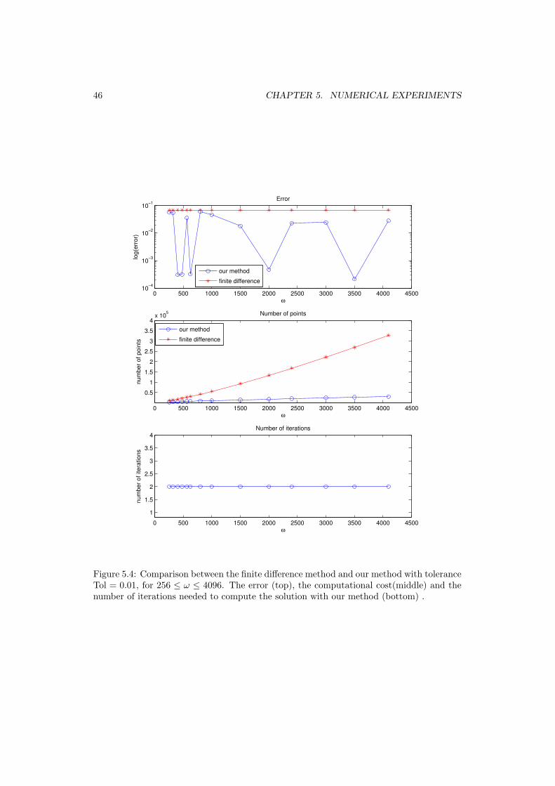
46 CHAPTER 5. NUMERICAL EXPERIMENTS
0 500 1000 1500 2000 2500 3000 3500 4000 450010−4
10−3
10−2
10−1Error
ω
log(
erro
r)
our methodfinite difference
0 500 1000 1500 2000 2500 3000 3500 4000 4500
0.51
1.52
2.53
3.54
x 105 Number of points
ω
num
ber o
f poi
nts
our methodfinite difference
0 500 1000 1500 2000 2500 3000 3500 4000 45001
1.5
2
2.5
3
3.5
4Number of iterations
ω
num
ber o
f ite
ratio
ns
Figure 5.4: Comparison between the finite difference method and our method with toleranceTol = 0.01, for 256 ≤ ω ≤ 4096. The error (top), the computational cost(middle) and thenumber of iterations needed to compute the solution with our method (bottom) .
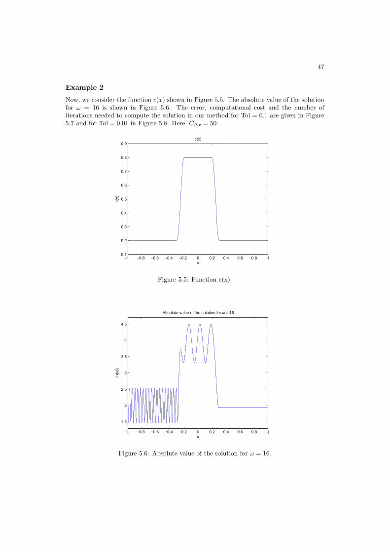
47
Example 2
Now, we consider the function c(x) shown in Figure 5.5. The absolute value of the solutionfor ω = 16 is shown in Figure 5.6. The error, computational cost and the number ofiterations needed to compute the solution in our method for Tol = 0.1 are given in Figure5.7 and for Tol = 0.01 in Figure 5.8. Here, C∆x = 50.
−1 −0.8 −0.6 −0.4 −0.2 0 0.2 0.4 0.6 0.8 10.1
0.2
0.3
0.4
0.5
0.6
0.7
0.8
0.9c(x)
x
c(x)
Figure 5.5: Function c(x).
−1 −0.8 −0.6 −0.4 −0.2 0 0.2 0.4 0.6 0.8 1
1.5
2
2.5
3
3.5
4
4.5
Absolute value of the solution for ω = 16
x
|u(x
)|
Figure 5.6: Absolute value of the solution for ω = 16.
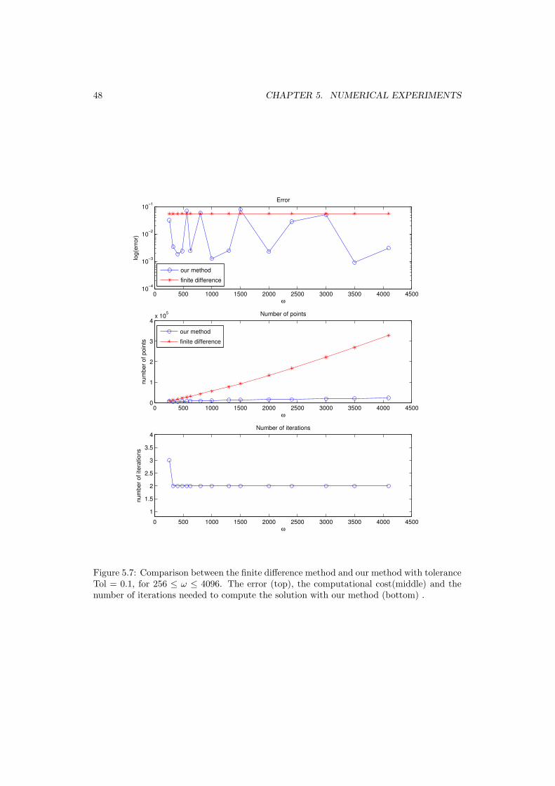
48 CHAPTER 5. NUMERICAL EXPERIMENTS
0 500 1000 1500 2000 2500 3000 3500 4000 450010−4
10−3
10−2
10−1Error
ω
log(
erro
r)
0 500 1000 1500 2000 2500 3000 3500 4000 45000
1
2
3
4x 10⁵ Number of points
ω
num
ber o
f poi
nts
0 500 1000 1500 2000 2500 3000 3500 4000 45001
1.5
2
2.5
3
3.5
4Number of iterations
ω
num
ber o
f ite
ratio
ns
our methodfinite difference
our methodfinite difference
Figure 5.7: Comparison between the finite difference method and our method with toleranceTol = 0.1, for 256 ≤ ω ≤ 4096. The error (top), the computational cost(middle) and thenumber of iterations needed to compute the solution with our method (bottom) .
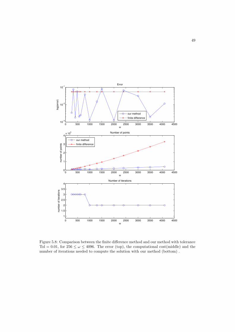
49
0 500 1000 1500 2000 2500 3000 3500 4000 450010−3
10−2
10−1Error
ω
log(
erro
r)
0 500 1000 1500 2000 2500 3000 3500 4000 45000
1
2
3
4x 10⁵ Number of points
ω
num
ber o
f poi
nts
0 500 1000 1500 2000 2500 3000 3500 4000 45001
1.5
2
2.5
3
3.5
4Number of iterations
ω
num
ber o
f ite
ratio
ns
our methodfinite difference
our methodfinite difference
Figure 5.8: Comparison between the finite difference method and our method with toleranceTol = 0.01, for 256 ≤ ω ≤ 4096. The error (top), the computational cost(middle) and thenumber of iterations needed to compute the solution with our method (bottom) .
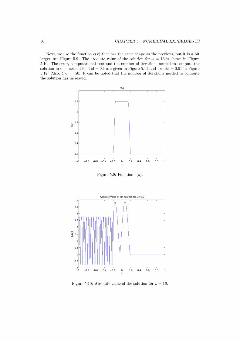
50 CHAPTER 5. NUMERICAL EXPERIMENTS
Next, we use the function c(x) that has the same shape as the previous, but it is a bitlarger, see Figure 5.9. The absolute value of the solution for ω = 16 is shown in Figure5.10. The error, computational cost and the number of iterations needed to compute thesolution in our method for Tol = 0.1 are given in Figure 5.11 and for Tol = 0.01 in Figure5.12. Also, C∆x = 50. It can be noted that the number of iterations needed to computethe solution has increased.
−1 −0.8 −0.6 −0.4 −0.2 0 0.2 0.4 0.6 0.8 1
0.2
0.4
0.6
0.8
1
1.2
c(x)
x
c(x)
Figure 5.9: Function c(x).
−1 −0.8 −0.6 −0.4 −0.2 0 0.2 0.4 0.6 0.8 10
0.5
1
1.5
2
2.5
3
3.5
4
4.5
5
x
|u(x
)|
Absolute value of the solution for ω = 16
Figure 5.10: Absolute value of the solution for ω = 16.

51
0 500 1000 1500 2000 2500 3000 3500 4000 450010−2
10−1
100Error
ω
log(
erro
r)
0 500 1000 1500 2000 2500 3000 3500 4000 45000
1
2
3
4x 10⁵ Number of points
ω
num
ber o
f poi
nts
0 500 1000 1500 2000 2500 3000 3500 4000 45001
2
3
4
5Number of iterations
ω
num
ber o
f ite
ratio
ns
our methodfinite difference
our methodfinite difference
Figure 5.11: Comparison between the finite difference method and our method with toler-ance Tol = 0.1, for 256 ≤ ω ≤ 4096. The error (top), the computational cost(middle) andthe number of iterations needed to compute the solution with our method (bottom) .
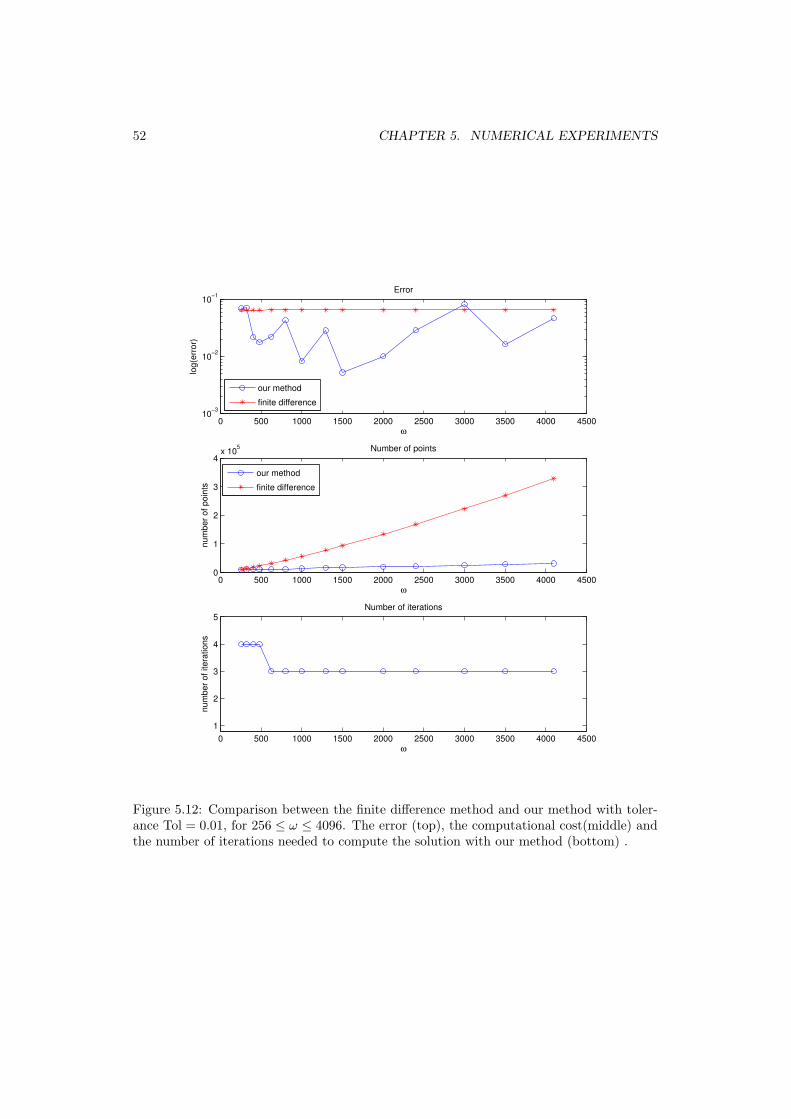
52 CHAPTER 5. NUMERICAL EXPERIMENTS
0 500 1000 1500 2000 2500 3000 3500 4000 450010−3
10−2
10−1Error
ω
log(
erro
r)
0 500 1000 1500 2000 2500 3000 3500 4000 45000
1
2
3
4x 10⁵ Number of points
ω
num
ber o
f poi
nts
0 500 1000 1500 2000 2500 3000 3500 4000 45001
2
3
4
5Number of iterations
ω
num
ber o
f ite
ratio
ns
our methodfinite difference
our methodfinite difference
Figure 5.12: Comparison between the finite difference method and our method with toler-ance Tol = 0.01, for 256 ≤ ω ≤ 4096. The error (top), the computational cost(middle) andthe number of iterations needed to compute the solution with our method (bottom) .
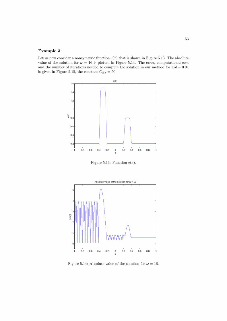
53
Example 3
Let us now consider a nonsymetric function c(x) that is shown in Figure 5.13. The absolutevalue of the solution for ω = 16 is plotted in Figure 5.14. The error, computational costand the number of iterations needed to compute the solution in our method for Tol = 0.01is given in Figure 5.15, the constant C∆x = 50.
−1 −0.8 −0.6 −0.4 −0.2 0 0.2 0.4 0.6 0.8 1
0.2
0.4
0.6
0.8
1
1.2
1.4
1.6c(x)
x
c(x)
Figure 5.13: Function c(x).
−1 −0.8 −0.6 −0.4 −0.2 0 0.2 0.4 0.6 0.8 1
0
1
2
3
4
5
x
|u(x
)|
Absolute value of the solution for ω = 16
Figure 5.14: Absolute value of the solution for ω = 16.

54 CHAPTER 5. NUMERICAL EXPERIMENTS
0 500 1000 1500 2000 2500 3000 3500 4000 450010−2
10−1
100Error
ω
log(
erro
r)
our methodfinite difference
0 500 1000 1500 2000 2500 3000 3500 4000 45000
1
2
3
4x 10⁵ Number of points
ω
num
ber o
f poi
nts
our methodfinite difference
0 500 1000 1500 2000 2500 3000 3500 4000 45002
3
4
5
6Number of iterations
ω
num
ber o
f ite
ratio
ns
Figure 5.15: Comparison between the finite difference method and our method with toler-ance Tol = 0.1, for 256 ≤ ω ≤ 4096. The error (top), the computational cost(middle) andthe number of iterations needed to compute the solution with our method (bottom) .
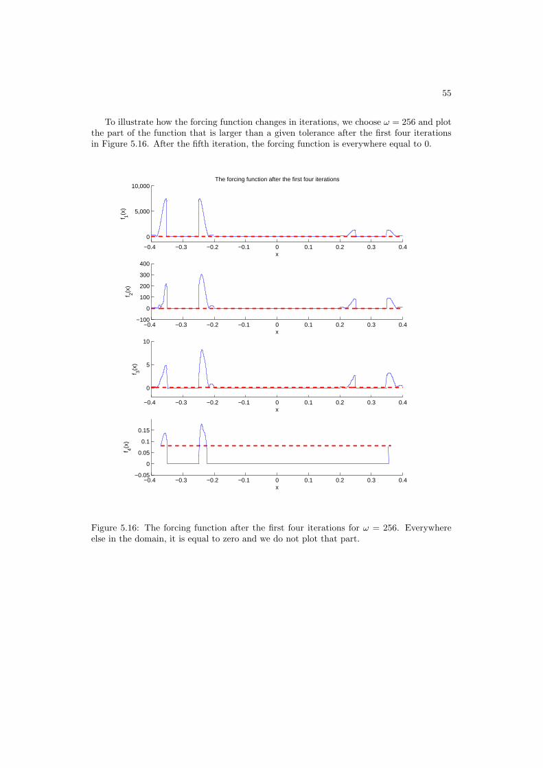
55
To illustrate how the forcing function changes in iterations, we choose ω = 256 and plotthe part of the function that is larger than a given tolerance after the first four iterationsin Figure 5.16. After the fifth iteration, the forcing function is everywhere equal to 0.
−0.4 −0.3 −0.2 −0.1 0 0.1 0.2 0.3 0.4
0
5,000
10,000
x
f 1(x)
The forcing function after the first four iterations
−0.4 −0.3 −0.2 −0.1 0 0.1 0.2 0.3 0.4−100
0
100
200
300
400
x
f 2(x)
−0.4 −0.3 −0.2 −0.1 0 0.1 0.2 0.3 0.4
0
5
10
x
f 3(x)
−0.4 −0.3 −0.2 −0.1 0 0.1 0.2 0.3 0.4−0.05
0
0.05
0.1
0.15
x
f 4(x)
Figure 5.16: The forcing function after the first four iterations for ω = 256. Everywhereelse in the domain, it is equal to zero and we do not plot that part.
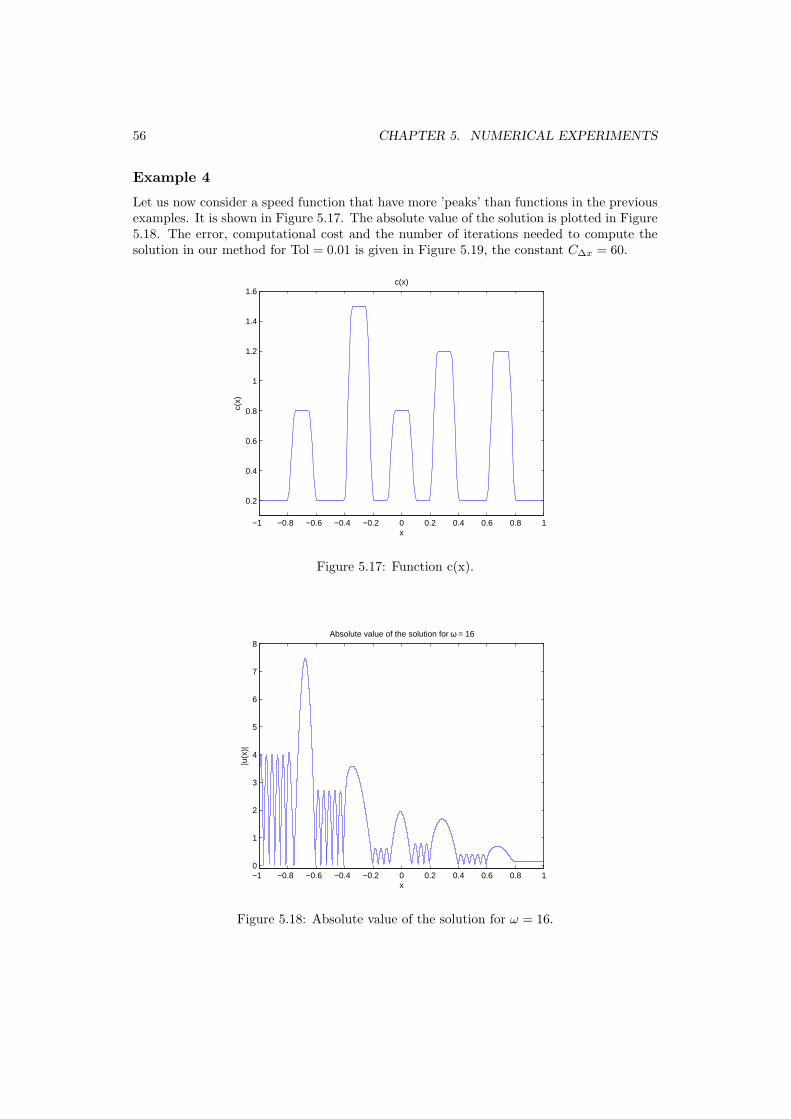
56 CHAPTER 5. NUMERICAL EXPERIMENTS
Example 4
Let us now consider a speed function that have more ’peaks’ than functions in the previousexamples. It is shown in Figure 5.17. The absolute value of the solution is plotted in Figure5.18. The error, computational cost and the number of iterations needed to compute thesolution in our method for Tol = 0.01 is given in Figure 5.19, the constant C∆x = 60.
−1 −0.8 −0.6 −0.4 −0.2 0 0.2 0.4 0.6 0.8 1
0.2
0.4
0.6
0.8
1
1.2
1.4
1.6c(x)
x
c(x)
Figure 5.17: Function c(x).
−1 −0.8 −0.6 −0.4 −0.2 0 0.2 0.4 0.6 0.8 10
1
2
3
4
5
6
7
8
x
|u(x
)|
Absolute value of the solution for ω = 16
Figure 5.18: Absolute value of the solution for ω = 16.

57
0 500 1000 1500 2000 2500 3000 3500 4000 450010
−2
10−1
100
Error
ω
log(
erro
r)
our methodfinite difference
0 500 1000 1500 2000 2500 3000 3500 4000 45000
1
2
3
4x 10
5 Number of points
ω
num
ber
of p
oint
s
our method
finite difference
0 500 1000 1500 2000 2500 3000 3500 4000 45001
2
3
4
5
6Number of iterations
ω
num
ber
of it
erat
ions
Figure 5.19: Comparison between the finite difference method and our method with toler-ance Tol = 0.01, for 256 ≤ ω ≤ 4096. The error (top), the computational cost(middle) andthe number of iterations needed to compute the solution with our method (bottom) .
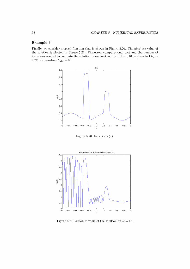
58 CHAPTER 5. NUMERICAL EXPERIMENTS
Example 5
Finally, we consider a speed function that is shown in Figure 5.20. The absolute value ofthe solution is plotted in Figure 5.21. The error, computational cost and the number ofiterations needed to compute the solution in our method for Tol = 0.01 is given in Figure5.22, the constant C∆x = 80.
−1 −0.8 −0.6 −0.4 −0.2 0 0.2 0.4 0.6 0.8 1
0.2
0.4
0.6
0.8
1
1.2
1.4
1.6c(x)
x
c(x)
Figure 5.20: Function c(x).
−1 −0.8 −0.6 −0.4 −0.2 0 0.2 0.4 0.6 0.8 10
0.5
1
1.5
2
2.5
3
3.5
4
4.5Absolute value of the solution for ω = 16
x
|u(x
)|
Figure 5.21: Absolute value of the solution for ω = 16.
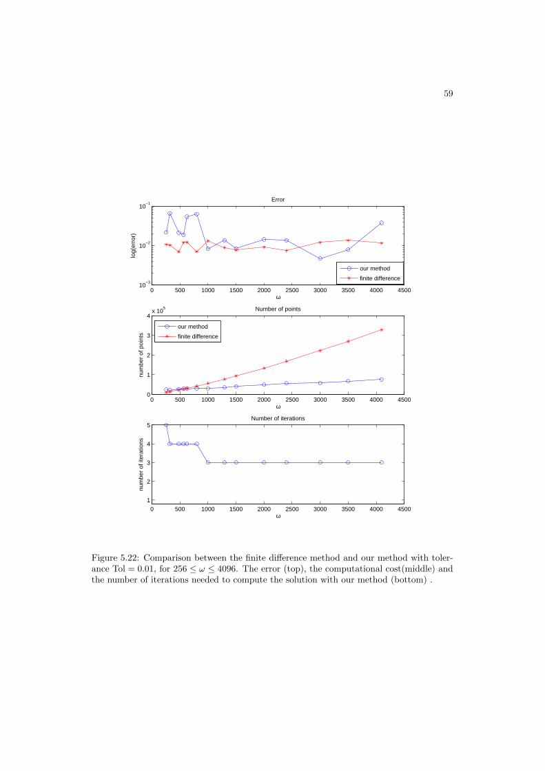
59
0 500 1000 1500 2000 2500 3000 3500 4000 450010
−3
10−2
10−1
Error
ω
log(
erro
r)
our method
finite difference
0 500 1000 1500 2000 2500 3000 3500 4000 45000
1
2
3
4x 10
5 Number of points
ω
num
ber
of p
oint
s
our method
finite difference
0 500 1000 1500 2000 2500 3000 3500 4000 4500
1
2
3
4
5Number of iterations
ω
num
ber
of it
erat
ions
Figure 5.22: Comparison between the finite difference method and our method with toler-ance Tol = 0.01, for 256 ≤ ω ≤ 4096. The error (top), the computational cost(middle) andthe number of iterations needed to compute the solution with our method (bottom) .

Bibliography
[1] T. Abboud, J.-C. Nedelec, and B. Zhou. Methode des ecuations integrales pour leshautes frequencies. C.R. Acad. Sci. Paris., 318:165–170, 1994.
[2] F. V. Atkinson. Wave propagation and the Bremmer series. J. Math. Anal. Appl., 1:225–276, 1960.
[3] V. M. Babic and T. F. Pankratova. On discontinuities of Green’s function of the waveequation with variable coefficient. Problemy Matem. Fiziki., Leningrad University,Saint-Petersburg, 6, 1973.
[4] R. Bellman and R. Kalaba. Functional equations, wave propagation and invariantimbedding. J. Math Mech., 8:683–704, 1959.
[5] H. Bremmer. The W.K.B. approximation as the first term of a geometric-optical series.Commun. Pure Appl. Math., 4:105–115, 1951.
[6] Y. Brenier and L. Corrias. A kinetic formulation for multibranch entropy solutions ofscalar conservations laws. Ann. Inst. Henri Poincare, 15(2):169–190, 1998.
[7] S. C. Brenner and L. R. Scott. The Mathematical Theory of Finite Element Methods.Springer, 2008.
[8] O. P. Bruno, C. A. Geuzaine, J. A. Monro Jr, and F. Reitich. Prescribed error toleranceswithin fixed computational times for scattering problems of arbitrarily high frequency:the convex case. Philos. Transact. A. Math. Phys. Eng. Sci., 362(1816):629–645, 2004.
[9] O. P. Bruno, C. A. Geuzaine, and F. Reitich. On the O(1) solution of multiple-scattering problems. IEEE Trans. Magn., 41:1488–1491, 2005.
[10] O. Cessenat and B. Despres. Application of an ultra weak variational formulation ofelliptic PDEs to the two-dimensional Helmholtz problem. SIAM J. Numer. Anal., 35(1):255–299, 1998.
[11] S. N. Chandler-Wilde and I. G. Graham. Boundary integral methods in high frequencyscattering. In B. Engquist, T. Fokas, E. Hairer, and A. Iserles, editors, Highly Oscil-latory Problems: Theory, Computation and Applications. Cambridge University Press,2008.
[12] V. Cerveny, I. A. Molotkov, and I. Psencik. Ray methods in seismology. Univ. KarlovaPress, 1977.
[13] B. Cockburn, G. Karniadakis, and C.-W. Shu. Discontinuous Galerkin Methods: the-ory, computations and applications, volume 11 of Lecture Notes in Computational Sci-ence and engineering. Springer, 2000.
61
62 BIBLIOGRAPHY
[14] D. Colton and R. Kress. Inverse Acoustic and Electromagnetic Scattering Theory,volume 93. Applied Mathematical Sciences, Springer-Verlag, Berlin, 1998.
[15] L Demanet and L. Ying. Wave atoms and time upscaling of wave equations. To appearin Numer.Math., 2007.
[16] V. Dominguez, I. G. Graham, and V. P. Smyshlyaev. A hybrid numerical-asymptoticboundary integral method for high-frequency acoustic scattering. Numer. Math., 106:471–510, 2007.
[17] F. Ecevit and F. Reitich. Analysis of multiple scattering iterations for high-frequencyscattering problems. Technical report, Max-Planck-Institut fur Mathematik in denNaturwissendchaften, Leipzig, 2006.
[18] H. C. Elman and D. P. O’Leary. Efficient iterative solution of the three-dimensionalHelmholtz equation. J. Comput. Phys., 142(1):163–181, 1998.
[19] B. Engquist, S. Osher, and S. Zhong. Fast wavelet based algorithms for linear evolutionequations. SIAM J. Sci. Comp., 15(4):755–775, 1994.
[20] B. Engquist and O. Runborg. Multiphase computations in geometrical optics. J.Comput. Appl. Math., 74:175–192, 1996.
[21] B. Engquist and O. Runborg. Computational high frequency wave propagation. ActaNumerica, 12:181–266, 2003.
[22] B. Engquist, O. Runborg, and A.-K. Tornberg. High-frequency wave propagation bythe segment projection method. J. Comput. Phys., 178:373–390, 2002.
[23] B. Engquist and L. Ying. Fast directional multilevel algorithms for oscillatory kernels.SIAM Journal on Scientific Computing, 29(4):1710–1737, 2007.
[24] K. Eriksson, D. Estep, P. Hansbo, and C. Johnson. Computational Differential Equa-tions. Studnetlitteratur, Lund, 1996.
[25] Y. A. Erlagga. Advances in iterative methods and preconditioners for the Helmholtzequation. Arch. Comput. Methods Eng., 15:37–66, 2008.
[26] Y. A. Erlagga, C. Oosterlee, and C. Vuik. A novel multigrid based preconditioner forheterogeneous Helmholtz problem. SIAM J. Sci. Comput., 27:1471–1492, 2006.
[27] O. Ernst and G. H. Golub. A domain decomposition approach to solving the Helmholtzequation with a radiating boundary condition. American Mathematical Society, Prov-idence, 15:177–192, 1994.
[28] E. Giladi and J. B. Keller. A hybrid numerical asymptotic method for scatteringproblems. Comput. Phys., 174:226–247, 2001.
[29] B. Gustafsson. High Order Difference Methods for Time Dependent PDE. Springer-Verlag Berlin Heidelberg, 2008.
[30] H. Han and Z. Huang. A tailored finite point method for the Helmholtz equation withhigh wave numbers in heterogeneous medium. J. Comp. Math., 26:728–739, 2008.
63
[31] J. Hesthaven, D. Gottlieb, and S. Gottlieb. Spectra Methods for Time-dependent Prob-lems, volume 21 of Cambridge Monographs on Applied and Computational Mathemat-ics. Cambridge University Press, 2007.
[32] D. Huybrechts and S. Vandewalle. A sparse discretisation for integral equation for-mulations of high-frequency scattering problems. Comm. SIAM J. Sci. Comput., 29:2305–2328, 2007.
[33] B. R. Julian and D. Gubbins. Three-dimensional seismic ray tracing. J. Geophys. Res.,43:95–114, 1977.
[34] H. B. Keller and J. B. Keller. Exponential-like solutions of systems of linear ordinarydifferential equations. J. SIAM, 10:246–259, 1962.
[35] J. Keller. Geometrical theory of diffraction. J. Opt. Soc. Amer, 52, 1962.
[36] R. Kress. Linear Integral Equations, volume 82 of Applied Mathematical Sciences.Springer-Verlag, second edition, 1999.
[37] R. T. Langan, I. Lerche, and R. T. Cutler. Tracing of rays through heterogeneousmedia: An accurate and efficient procedure. Geophysics, 50:1456–1465, 1985.
[38] S. Langdon and S. N. Chandler-Wilde. A wave number independent boundary elementmethod for an acoustic scattering problem. SIAM J. Num. Anal., 43:2450–2477, 2006.
[39] E. Larsson. A domain decomposition method for the Helmholtz equation in a multilayerdomain. SIAM J. Sci. Comput., 20(5):1713–1731, 1999.
[40] Randall. J. LeVeque. Finite Volume Methods for Hyperbolic Problems. CambridgeUniversity Press, 2006.
[41] J. Lundstedt and S. He. Time domain direct and inverse problems for a nonuniformLCRG line with internal sources. IEEE Transactions on Electromagnetic Compatibility,39(2):79–88, 1997.
[42] H. McMaken. On the convergence of the Bremmer series for the Helmholtz equationin 2-D. Wave Motion, 8:277–283, 1986.
[43] Made MMM. Incomplete factorization-based preconditionings for solving theHelmholtz equation. Int. J. Numer. Methods Eng., 50:1077–1101, 2001.
[44] M. Motamed and O. Runborg. Taylor expansion errors in gaussian beam summation.Preprint, KTH, 2008.
[45] S. J. Osher and J. A. Sethian. Fronts propagating with curvature-dependent speed:Algorithms based on Hamilton-Jacobi formulations. J. Comput. Phys., 79(1):12–49,1988.
[46] S. J. Osher and C.-W. Shu. High–order essentially nonoscillatory schemes for Hamilton-Jacobi equations. SIAM J. Numer. Anal., 28(4):907–977, 1991.
[47] K. Otto and E. Larsson. Iterative solution of the Helmholtz equation by a second–ordermethod. SIAM J. Matrix Anal. Appl., 21(1):209–229, 1999.
64 BIBLIOGRAPHY
[48] E. Perrey-Debain, O. Laghrouche, P. Bettess, and J. Trevelyan. Plane-wave basis finiteelements and boundary elements for three-dimensional wave scattering. Philos. Trans.R. Soc. Lond. Ser. A Math. Phys. Eng. Sci., 362(1816):561–577, 2004.
[49] M. M. Popov. A new method of computation of wave fields using gaussian beams.Wave Motion, 4:85–97, 1982.
[50] V. Rokhlin. Sparse diagonal forms for translation operators for the Helmholtz equationin two dimensions. Appl. Comput. Harmon. Anal., 5(1):36–67, 1998.
[51] O. Runborg. Some new results in multiphase geometrical optics. M2AN Math. Model.Numer. Anal., 34:1203–1231, 2000.
[52] O. Runborg. Mathematical models and numerical methods for high frequency waves.Communications in Computational Physics, 2(5):827–880, 2007.
[53] J. A. Sethian. A fast marching level set method for monotonically advancing fronts.Proc. Nat. Acad. Sci. U.S.A., 93(4), 1966.
[54] Christiaan C. Stolk. A fast method for linear waves based on geometrical optics. SIAMJ. Numer. Anal., 47:1168–1194, 2009.
[55] A. Taflove. Computational Electrodynamics: The Finite-Difference Time-DomainMethod. Norwood, MA: Artech House, 1995.
[56] A. Taflove and S. C. Hagness. Computational Electrodynamics: The Finite-DifferenceTime-Domain Method. Norwood, MA: Artech House, second edition, 2000.
[57] C. H. Thurber and W. L. Ellsworth. Rapid solution of ray tracing problems in hetero-geneous media. Bull. Seism. Soc. Amer., 70:1147–1148, 1980.
[58] A.-K. Tornberg and B. Engquist. The segment projection method for interface tracking.Comm. Pure Appl. Math., 56(1):47–79, 2003.
[59] L. N. Trefethen. Spectral Methods in MATLAB. SIAM, 2000.
[60] Y. R. Tsai, L. T. Cheng, S. Osher, and H. K. Zhao. Fast sweeping algorithms for a classof Hamilton-Jacobi equations. SIAM Journal on Numerical Analysis, 41(2):673–694,2003.
[61] J. N. Tsitsiklis. Efficient algorithms for globally optimal trajectories. IEEE Trans.Automat. Control, 40(9):1528–1538, 1995.
[62] G. B. Whitham. Linear and nonlinear waves. John Wiley & Sons, Inc., 1974.
[63] Kane S. Yee. Numerical solution of initial boundary value problems involving Maxwell’sequations in isotropic media. IEEE Trans. Antennas Propagat., AP-14(3):302–307,1966.
Appendix A
Runge–Kutta Schemes for LinearScalar Problems
We consider the linear scalar ordinary differential equation
y′ = iωa(x, ω)y + b(x, ω), y(0) = y0. (A.1)
We solve it with a p-th order explicit s-stage Runge–Kutta scheme, where 0 ≤ p ≤ s,described by
ξ1 = iωa(xn, ω)y(xn) + b(xn, ω),
and for j = 2, . . . , s,
ξj = iωa(xn + γj∆x, ω)
(y(xn) + ∆x
j−1∑`=1
αj,`ξ`
)+ b(xn + γj∆x, ω).
Finally,
yn+1 = y(xn) + ∆xs∑j=1
βjξj .
We are interested in characterizing the error in one step, the local truncation error:
τn := y(xn + ∆x)− yn+1.
Since the method is of p-th order, the first p terms in the Taylor expansion of τn around∆x = 0 are zero. Throughout this section we will assume that b(·, ω) ∈ Cp+1(R) for all ωand a(·, ω) ∈ Cp+1(R) uniformly in ω, i.e. that
supx,ω∈R
|∂kxa(x, ω)| ≤ C, k = 0, . . . , p+ 1.
This means in particular that the solution y(x) ∈ Cp+2. We can then prove the following
Theorem 6. Suppose ∆xω ≤ 1 and ω ≥ 1. Then the local truncation error can be estimatedas
|τn| ≤ C ∆xp+1
p+1∑`=0
|y(p+1−`)|∞ω`,
where the constant is independent of x, ω, y(x) and b(x, ω).
65
66 APPENDIX A. RUNGE–KUTTA SCHEMES FOR LINEAR SCALAR PROBLEMS
To prove this theorem we introduce a space Cpb to denote functions of the form c(x, ω,∆x)which are p times continuously differentiable in ∆x with uniform bounds on the derivativesin x and ω,
supx,ω∈R
|∂k∆xc(x, ω,∆x)| ≤ C, k = 0, . . . , p.
In particular a(x + α∆x, ω) ∈ Cp+1b for all α. We then let Pd be functions f(z, x, ω,∆x)
which are polynomials of degree d in z,
f(z, x, ω,∆x) = c0(x, ω,∆x) + zc1(x, ω,∆x) + · · ·+ zdcd(x, ω,∆x),
and where the coefficients cj ∈ Cp+1b . We then have the following lemma characterizing the
form of the Runge–Kutta scheme.
Lemma 9. The Runge–Kutta scheme can be written in the following form
yn+1 = yn + ∆x
iωa(iω∆x, xn, ω,∆x)yn +s∑j=1
rj(iω∆x, xn, ω,∆x)b(xn + γj∆x, ω)
,where a ∈ Ps−1 and rj ∈ Ps−j do not depend on ω, yn or b(x, ω).
Proof. Let
aj(x, ω,∆x) = a(x+ γj∆x, ω), bj(x, ω,∆x) = b(x+ γj∆x, ω),
so that a(x) = a1(x, ω,∆x), b(x) = b1(x, ω,∆x). We note that aj ∈ Cp+1b by our assump-
tions. We haveξ1 = iωa1yn + b1,
and for j = 2, . . . , s,
ξj = iωaj
(yn + ∆x
j−1∑`=1
αj,`ξ`
)+ bj .
We claim that there are qj ∈ Pj−1 and rj,k ∈ Pj−k such that
ξj = iωqj(iω∆x, xn, ω,∆x)yn +j∑
k=1
rj,k(iω∆x, xn, ω,∆x)bk.
This is true for j = 1 since we can take q1 = a1 and r1,1 = 1. For j > 1,
ξj = iωaj
(yn + ∆x
j−1∑`=1
αj,`
[iωq`yn +
∑k=1
r`,kbk
])+ bj
= iωaj
(1 + iω∆x
j−1∑`=1
αj,`q`
)yn + iω∆xaj
j−1∑`=1
∑k=1
αj,`r`,kbk + bj
= iωaj
(1 + iω∆x
j−1∑`=1
αj,`q`
)yn + iω∆xaj
j−1∑k=1
bk
j−1∑`=k
αj,`r`,k + bj .
67
Thus, rj,j = 1 and
qj(z, x, ω,∆x) = aj(x, ω,∆x)
(1 + z
j−1∑`=1
αj,`q`(z, x, ω,∆x)
),
rj,k(z, x, ω,∆x) = zaj(x, ω,∆x)j−1∑`=k
αj,`r`,k(y, x, ω,∆x).
Clearly, if q` ∈ P`−1 and r`,k ∈ P`−k for 1 ≤ k ≤ ` < j, then the same holds also for1 ≤ k ≤ ` = j, showing the claim by induction. Finally,
yn+1 = yn + ∆xs∑j=1
βjξj = yn + ∆xs∑j=1
βj
[iωqjyn +
j∑k=1
rj,kbk
].
Hence,
a =s∑j=1
βjqj , rk =s∑j=k
βjrj,k. (A.2)
Since qj ∈ Pj−1 and rj,k ∈ Pj−k this proves the lemma.
Before continuing, we introduce the Taylor expansion polynomial for c(∆x) ∈ Cp+1(R).More precisely, we let Tkc be the Taylor polynomial of degree k ≤ p around ∆x = 0, definedas
(Tkc)(z) :=k∑`=0
z`∂
(`)∆xc(0)`!
,
so that
|c(∆x)− (Tkc)(∆x)| ≤ ∆xk+1
`!sup
0≤ξ≤∆x
∣∣∣∂(k+1)∆x c(ξ)
∣∣∣ .We note that in particular if we apply Tk to a function c(x, ω,∆x) ∈ Cp+1
b then
|c(x, ω,∆x)− (Tkc)(x, ω,∆x)| ≤ sup0≤ξ≤∆x
∣∣∣∂(k+1)∆x c(x, ω, ξ)
∣∣∣ ≤ C ∆xk+1,
where the constant C is independent of x and ω.We will also let Qd be another polynomial space similar to Pd but where the functions
are of the form
f(x, ω,∆x) = c0(x, ω) + c1(x, ω)∆x+ · · ·+ cd(x, ω)∆xd,
and the coefficients cj ∈ Cp+1 for each ω, but not necessarily bounded uniformly in ω.
Lemma 10. For each f ∈ Pd, y ∈ Cp+1(R) and integer p ≥ 0 there exists f ∈ Qp such that∣∣f(iω∆x, x, ω,∆x)y(x+ α∆x)− f(x, ω,∆x)∣∣
≤ C
(∆xp+1
p+1∑`=0
∑k=0
|y(`−k)|∞ωk + (∆xω)max(d,p+1)|y|∞
), (A.3)
where C is independent of x, ω, ∆x and y(x).

68 APPENDIX A. RUNGE–KUTTA SCHEMES FOR LINEAR SCALAR PROBLEMS
Proof. Since f ∈ Pd we can write the function as
f(z, x, ω,∆x)y(x+ α∆x) =d∑k=0
ck(x, ω,∆x)y(x+ α∆x)zk.
where ck ∈ Cp+1b . With q = min(d, p) we divide the sum into three parts
f(iω∆x, x, ω,∆x)y(x+ α∆x) =q∑
k=0
ck(x, ω,∆x)(Tp−ky)(x,∆x)(iω∆x)k
+q∑
k=0
ck(x, ω,∆x)[(Tp−ky)(x,∆x)− y(x+ α∆x)](iω∆x)k
+d∑
k=q+1
ck(x, ω,∆x)y(x+ α∆x)(iω∆x)k
=: E1 + E2 + E3,
where E3 = 0 if p ≥ d. We start by considering E1. Let f` ∈ Qp−` be defined as
f`(x, ω,∆x) =min(q,`)∑k=0
p−∑r=0
∆xr∂
(r)∆xck(x, ω, 0)
r!Y`−k(x)(iω)k =
min(q,`)∑k=0
(Tp−`ck)(x, ω,∆x)Y`−k(x)(iω)k,
where Y`(x) := α`y(`)(x)/`!. Then,
E1 =q∑
k=0
p−k∑`=0
ck(x, ω,∆x)∆x`Y`(x)(iω∆x)k =p∑`=0
∆x`min(q,`)∑k=0
ck(x, ω,∆x)Y`−k(x)(iω)k
=p∑`=0
∆x`f`(x, ω,∆x) +p∑`=0
∆x`min(q,`)∑k=0
[ck(x, ω,∆x)− (Tp−`ck)(x, ω,∆x)]Y`−k(x)(iω)k.
We have furthermore
min(q,`)∑k=0
[ck(x, ω,∆x)− (Tp−`ck)(x, ω,∆x)]Y`−k(x)(iω)k ≤ C∆xp−`+1
min(q,`)∑k=0
|y(`−k)|∞ωk,
where C is independent of y(x). Thus, defining
f(x, ω,∆x) :=p∑`=0
f`(x, ω,∆x)∆x` ∈ Qp,
we get
|f(iω∆x, x, ω,∆x)y(x+α∆x)−f(x, ω,∆x)| ≤ C∆xp+1
p∑`=0
min(q,`)∑k=0
|y(`−k)|∞ωk+|E2|+|E3|.
For E2 we can estimate |Tp−ky − y| ≤ Ck|y(p−k+1)|∞∆xp−k+1 to get,
|E2| ≤ C∆xp+1
q∑k=0
|y(p−k+1)|∞ωk,
69
and for E3 we trivially have
|E3| ≤ C|y|∞d∑
k=p+1
(ω∆x)k ≤ C|y|∞[(ω∆x)p+1 + (ω∆x)d
],
when p < d. The result follows from these estimates.
Corollary 2. Suppose ∆xω ≤ 1 and ω ≥ 1. Then, for each f ∈ Pd, y ∈ Cp+1(R) andinteger p ≥ 0 there exists f ∈ Qp such that
∣∣f(iω∆x, x, ω,∆x)y(x+ α∆x)− f(x, ω,∆x)∣∣ ≤ C ∆xp+1
p+1∑`=0
|y(p+1−`)|∞ω`,
where C is independent of x, ω, ∆x and y(x).
Proof. When ω ≥ 1,
p+1∑`=0
∑k=0
|y(`−k)|∞ωk =p+1∑`=0
∑k=0
|y(p+1−`)|∞ωk ≤ (p+ 1)p+1∑`=0
|y(p+1−`)|∞ω`. (A.4)
Moreover, when ∆xω ≤ 1, clearly (∆xω)max(d,p+1)|y|∞ ≤ (∆xω)p+1|y|∞, which is alreadyincluded in the first error term of (A.3).
Proof of Theorem 6
From Lemma 9 and the equation (A.1) we have that
yn+1 =yn + ∆x
iωa(iω∆x, xn, ω,∆x)yn +s∑j=1
rj(iω∆x, xn, ω,∆x)b(xn + γj∆x, ω)
=[1 + iω∆xa(iω∆x, xn, ω,∆x)]yn + ∆x
s∑j=1
rj(iω∆x, xn, ω,∆x)y′(xn + γj∆x)
+s∑j=1
sj(iω∆x, xn, ω,∆x)y(xn + γj∆x),
where
sj(z, xn, ω,∆x) = −zrj(z, xn, ω,∆x)a(xn + γj∆x, ω) ∈ Ps+1−j .
We also note that [1+za(z, x, ω,∆x)] ∈ Ps and rj ∈ Ps−j . Since also y ∈ Cp+2 the result inCorollary 2 shows that we can approximate [1+iω∆xa(iω∆x, xn,∆x)]yn, rj(iω∆x, xn,∆x)y′(xn+γj∆x), and sj(iω∆x, xn,∆x)y(xn + γj∆x) in the sense of (A.4) by some functions a ∈ Qp,

70 APPENDIX A. RUNGE–KUTTA SCHEMES FOR LINEAR SCALAR PROBLEMS
rj ∈ Qp−1 and sj ∈ Qp respectively. Then
τn+1 = y(xn+1)− yn+1 = (Tpy)(xn, ω,∆x)− a(xn, ω,∆x)−∆xs∑j=1
rj(xn, ω,∆x)
+ y(xn+1)− (Tpy)(xn,∆x)+ a(xn, ω,∆x)− [1 + iω∆xa(iω∆x, xn, ω,∆x)]yn
+ ∆xs∑j=1
[rj(xn, ω,∆x)− rj(iω∆x, xn, ω,∆x)y′(xn + γj∆x)]
+s∑j=1
[sj(xn, ω,∆x)− sj(iω∆x, xn, ω,∆x)y(xn + γj∆x)]
=: E1 + E2 + E3 + E4 + E5.
For E2,|E2| ≤ C∆xp+1|y(p+1)|∞.
We can now use (A.4) in Corollary 2 to bound the therms E3, E4 and E5. In E3 the functiony is constant so,
|E3| ≤ C ∆xp+1ωp+1|y|∞.
For E4 we apply it to the derivative of y(x),
|E4| ≤ C ∆xp+1
p∑`=0
y(p+1−`)|∞ω`,
and finally,
|E5| ≤ C ∆xp+1
p+1∑`=0
|y(p+1−`)|∞ω`.
Thus,5∑j=2
Ej ≤ C ∆xp+1
p+1∑`=0
|y(p+1−`)|∞ω`.
Since E1 is a polynomial in ∆x of order p and the method is of order p the term E1 mustvanish. This concludes the proof.


![Unique continuation for the Helmholtz equation using a ... · Unique continuation for the Helmholtz equation using ... I Laplace equation [Burman’14] ... Unique continuation for](https://static.documents.pub/doc/80x56/5ae0fc9a7f8b9a595d8b4a83/unique-continuation-for-the-helmholtz-equation-using-a-continuation-for-the.jpg)


![Green’s Functionof3-D Helmholtz Equation for … · arXiv:math/0408186v1 [math.AP] 13 Aug 2004 Green’s Functionof3-D Helmholtz Equation for Turbulent Medium: Application toOptics](https://static.documents.pub/doc/80x56/5b85b6787f8b9af12d8b5a65/greens-functionof3-d-helmholtz-equation-for-arxivmath0408186v1-mathap.jpg)

