A fast finite difference method for biharmonic equations on

irregular domains

Guo Chen ∗ Zhilin Li † Ping Lin ‡

Abstract

Biharmonic equations have many applications, especially in fluid and solid mechanics,but difficult to solve due to the fourth order derivatives in the differential equation. In thispaper a fast second order accurate algorithm based on a finite difference discretizationand a Cartesian grid is developed for two dimensional biharmonic equations on irregulardomains with essential boundary conditions. The irregular domain is embedded into arectangular region and the biharmonic equation is decoupled to two Poisson equations.An auxiliary unknown quantity ∆u along the boundary is introduced so that fast Poissonsolvers on irregular domains can be used. Non-trivial numerical example show the effi-ciency of the proposed method. The number of iterations of the method is independent ofthe mesh size. Another key to the method is a new interpolation scheme to evaluate theresidual of the Schur complement system. The new biharmonic solver has been appliedto solve the incompressible Stokes flow on an irregular domain.

1 Introduction

In this paper, we consider a biharmonic equation defined on an irregular domain Ω

∆2u(x, y) = f(x, y), (x, y) ∈ Ω,

u(x, y) = g1(x, y), (x, y) ∈ ∂Ω, (1.1)

un(x, y) = g2(x, y), (x, y) ∈ ∂Ω,

where

∆2 ≡ ∇4 =∂4

∂x4+ 2

∂4

∂x2∂y2+

∂4

∂y4, (1.2)

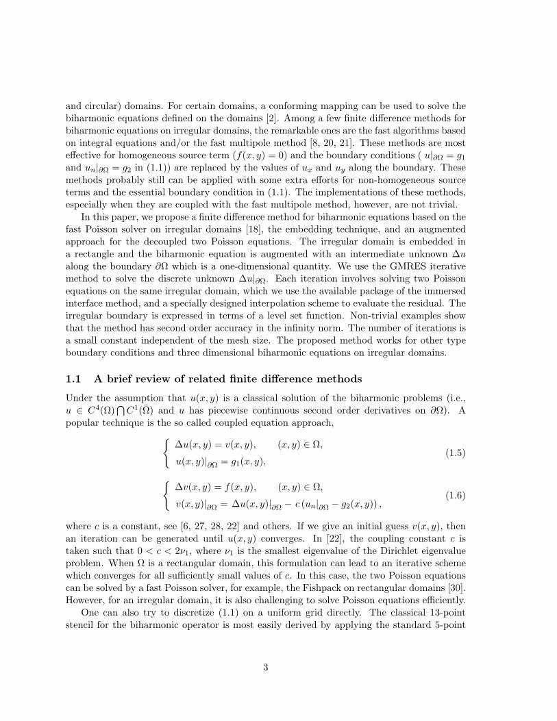
Ω is a bounded open set in R2 with a smooth boundary ∂Ω, un = ∂u∂n is the normal derivative

of u on ∂Ω, and n is the unit normal derivative pointing outward, see Fig. 1 for an illustration.∗Department of Mathematics, North Carolina State University, Raleigh, NC 27695, e-mail:

gchen@unity.ncsu.edu.†Center for Research in Scientific Computation & Department of Mathematics, North Carolina State

University, Raleigh, NC 27695, e-mail: zhilin@math.ncsu.edu.‡Department of Mathematics, National University of Singapore, 2 Science Drive 2, Singapore 117543,

e-mail: matlinp@nus.edu.sg.

1

Ω

u(x,y) = f(x,y)2

u = g (x,y)1

u = g (x,y)n 2

∆

Figure 1: A diagram of the problem: a biharmonic equation on an irregular domain.

Biharmonic equations arise in many applications. Classical examples can be found inelasticity, fluid mechanics, and many other areas. In fluid mechanics, the solution u(x, y)of equation (1.1) can be used to describe the stream-function of an incompressible two-dimensional creeping flow (zero Reynolds number), see Section 5 and [5, 15] for example. Inlinear elasticity, u(x, y) can be used to represent the airy stress function, see [32]. In thetheory of thin plates, equation (1.1) can be used to represent a “clamped plate” where f isthe external load, and the solution u(x, y) is the vertical displacement.

If the second boundary condition in (1.1) is replaced by ∆u|∂Ω = g2(x, y), then thebiharmonic equation can be decoupled as two Poisson equations with a Dirichlet boundarycondition on the same irregular domain

∆v(x, y) = f(x, y), (x, y) ∈ Ω,

v(x, y)|∂Ω = g2(x, y),(1.3)

∆u(x, y) = v(x, y), (x, y) ∈ Ω,

u(x, y)|∂Ω = g1(x, y).(1.4)

This observation is one of basis of our numerical method in which we set ∆u|∂Ω as anintermediate variable. It is much more difficult to solve the problem when un is prescribedalong ∂Ω.

Various numerical methods have been developed for biharmonic equations in the literaturewhen u and un are prescribed along ∂Ω. One approach is to use a body fitted mesh witha finite element discretization. The discrete system then can be solved using a multigridmethod, see [1, 4, 11, 31] for example. There is not much difference between regular orirregular domains in finite element methods except for the cost in the mesh generation andthe condition number of the discrete system of equations.

There are limited publications on finite difference methods for biharmonic equations onirregular domains, even fewer with convincing numerical examples. Most of the finite differ-ence methods appeared in the literature are for biharmonic equations on regular (rectangular

2

and circular) domains. For certain domains, a conforming mapping can be used to solve thebiharmonic equations defined on the domains [2]. Among a few finite difference methods forbiharmonic equations on irregular domains, the remarkable ones are the fast algorithms basedon integral equations and/or the fast multipole method [8, 20, 21]. These methods are mosteffective for homogeneous source term (f(x, y) = 0) and the boundary conditions ( u|∂Ω = g1

and un|∂Ω = g2 in (1.1)) are replaced by the values of ux and uy along the boundary. Thesemethods probably still can be applied with some extra efforts for non-homogeneous sourceterms and the essential boundary condition in (1.1). The implementations of these methods,especially when they are coupled with the fast multipole method, however, are not trivial.

In this paper, we propose a finite difference method for biharmonic equations based on thefast Poisson solver on irregular domains [18], the embedding technique, and an augmentedapproach for the decoupled two Poisson equations. The irregular domain is embedded ina rectangle and the biharmonic equation is augmented with an intermediate unknown ∆ualong the boundary ∂Ω which is a one-dimensional quantity. We use the GMRES iterativemethod to solve the discrete unknown ∆u|∂Ω. Each iteration involves solving two Poissonequations on the same irregular domain, which we use the available package of the immersedinterface method, and a specially designed interpolation scheme to evaluate the residual. Theirregular boundary is expressed in terms of a level set function. Non-trivial examples showthat the method has second order accuracy in the infinity norm. The number of iterations isa small constant independent of the mesh size. The proposed method works for other typeboundary conditions and three dimensional biharmonic equations on irregular domains.

1.1 A brief review of related finite difference methods

Under the assumption that u(x, y) is a classical solution of the biharmonic problems (i.e.,u ∈ C4(Ω)

⋂C1(Ω) and u has piecewise continuous second order derivatives on ∂Ω). A

popular technique is the so called coupled equation approach,∆u(x, y) = v(x, y), (x, y) ∈ Ω,

u(x, y)|∂Ω = g1(x, y),(1.5)

∆v(x, y) = f(x, y), (x, y) ∈ Ω,

v(x, y)|∂Ω = ∆u(x, y)|∂Ω − c (un|∂Ω − g2(x, y)) ,(1.6)

where c is a constant, see [6, 27, 28, 22] and others. If we give an initial guess v(x, y), thenan iteration can be generated until u(x, y) converges. In [22], the coupling constant c istaken such that 0 < c < 2ν1, where ν1 is the smallest eigenvalue of the Dirichlet eigenvalueproblem. When Ω is a rectangular domain, this formulation can lead to an iterative schemewhich converges for all sufficiently small values of c. In this case, the two Poisson equationscan be solved by a fast Poisson solver, for example, the Fishpack on rectangular domains [30].However, for an irregular domain, it is also challenging to solve Poisson equations efficiently.

One can also try to discretize (1.1) on a uniform grid directly. The classical 13-pointstencil for the biharmonic operator is most easily derived by applying the standard 5-point

3

Laplace’s operator twice

∆213ui,j =L5(L5ui,j) =

2h4

(20ui,j − 8(ui+1,j + ui−1,j + ui,j+1

+ ui,j−1) + 2(ui+1,j+1 + ui−1,j+1 + ui−1,j−1 + ui+1,j−1)+ (ui+2,j + ui−2,j + ui,j+2 + ui,j−2)).

(1.7)

The local truncation error is order of h2. The finite difference approximation above needsto be modified at grid points near the boundary. One popular choices is the quadraticextrapolation where the normal derivative boundary condition at the grid points near theboundary are used to extrapolated the ‘missing’ (exterior) point in the 13 point stencil. Thisresults in a stencil of the form:

∆2ui,j =2h4

(21ui,j − 8(ui+1,j + ui−1,j + ui,j+1

+ ui,j−1) + 2(ui+1,j+1 + ui−1,j+1 + ui−1,j−1 + ui+1,j−1)+ (ui+2,j + ui,j+2 + ui,j−2)) + 2hun(xi−1, yj),

(1.8)

when the irregular point uij is adjacent to the left boundary.Glowinski and Pironneau [7] made the observation that the 13-point finite difference

scheme combined with a quadratic extrapolation formula near the boundary is equivalent tosolving the biharmonic equation using a mixed finite element method with piecewise linearelements.

Many similar modifications are discussed in [10]. Proper treatment of the points nearthe boundary remains a challenging problem with these schemes since inaccurate boundaryapproximations may affect the accuracy, but too complicated boundary approximations maydestroy the matrix structure.

There are other alternative finite difference approximations for the biharmonic operator.Certain second and fourth-order finite difference approximations for the biharmonic equation(1.1) on a 9-point compact stencil are given in [29]. The approach there involves discretizingthe biharmonic equation (1.1) using not only the grid values of the unknown solution u(x, y)but also the values of the gradients ux(x, y) and uy(x, y) at selected grid points.

The standard iterative methods suffer from slow convergence when used to solve thesystem of finite difference equations for biharmonic equations, see for example, [9]. Directsolvers can only be used for relatively coarse grids. Bjørstad [24] had introduced a newiterative method that requires only O(N2) arithmetic operations on a rectangular domain,where N is the number of grid lines in one coordinate direction.

Due to the difficulties in handling the finite difference approximation close to a curvedboundary, all the finite difference methods discussed above are restricted to rectangular do-mains. It is the purpose of this paper to provide an efficient finite difference method forbiharmonic equations on irregular domains. An advantage using a Cartesian grid instead ofa body fitted grid is that there is almost no cost in the grid generation which is significant forfree boundary and moving interface problems that involving solving a biharmonic equation.

The paper is organized as follows. In Section 2, we introduce the main algorithm andthe fast Poisson solver for irregular domains. The interpolation scheme to evaluate the

4

residual of the Schur complement system is explained in Section 3. Numerical examples withgrid refinement and efficiency analysis are presented in Section 4. The application to theincompressible Stokes flow is presented in Section 5.

2 The numerical method based on an augmented approach

Consider the solution of the following problem∆v(x, y) = f(x, y), (x, y) ∈ Ω

v(x, y)|∂Ω = g(x, y),∆u(x, y) = v(x, y), (x, y) ∈ Ω

u(x, y)|∂Ω = g1(x, y).

(2.9)

The solution apparently is a functional of g(x, y) which is defined only along the boundary∂Ω. We denote the solution as ug(x, y) to express the dependency of the solution on g(x, y).

Let the solution of the original problem (1.1) be u∗(x, y), and define

g∗(x, y) = ∆u∗(x, y), (x, y) ∈ ∂Ω. (2.10)

Then u∗(x, y) satisfies the second Poisson equation in (1.1) with g(x, y) ≡ g∗(x, y). In otherwords, ug∗(x, y) ≡ u∗(x, y) and

∂u∗(x, y)∂n

∣∣∣∣∂Ω

= g2(x, y) (2.11)

is satisfied. Therefore, solving the original problem (1.1) is equivalent to finding the corre-sponding g∗(x, y) and then ug∗(x, y) in (2.9). Notice that g∗(x, y) is only defined along theboundary, so it is one dimensional lower than the solution u(x, y).

We call g(x, y) an augmented (intermediate) variable along the boundary. The auxiliaryequation then is

∂ug(x, y)∂n

∣∣∣∣∂Ω

= g2(x, y). (2.12)

Therefore the system is still closed since we have one more variable and one more equation.The idea is to start with a guess g(k)(x, y) as an approximation to g∗(x, y). Once we know

g(k)(x, y), we can solve the two Poisson equations in (2.9) to get the solution u(k)g (x, y). From

the residual equation (2.12), we hope to get a better approximation g(k+1)(x, y). The processwill become clearer after we discretize the system (2.9) and (2.12) in this section.

2.1 The computational frame

We embed the irregular domain into a rectangular domain R : [a, b]× [c, d] ⊃ Ω. The originalboundary ∂Ω then becomes an interface within R. We solve the two Poisson equations in

5

(2.9) on a uniform Cartesian grid

xi = a + ih, 0 ≤ i ≤ m,

yj = c + jh, 0 ≤ j ≤ n,(2.13)

where, for simplicity, we assume that h = (b − a)/m = (d − c)/n. The boundary ∂Ω isexpressed as the zero level set of a two dimensional function ϕ(x, y) defined on the entirerectangular region

ϕ(x, y)

> 0, if (x, y) ∈ R− Ω,

= 0, if (x, y) ∈ ∂Ω,

< 0, if (x, y) ∈ Ω.

(2.14)

There are a number of advantages using the level set method especially for complicatedgeometries and high dimensions. We refer the readers to [23, 26] for more information on thelevel set method.

The level set function is defined at all grid points by ϕij = ϕ(xi, yj). It is important thatϕ(x, y) be a good approximation to the signed distance function at least in the neighborhoodof the boundary ∂Ω. If the level set function is not a good approximation to the signeddistance function, then a re-initialization is needed to make it a good approximation to thesigned distance function, see [12, 13, 14] for the re-initialization process.

Using the grid function ϕij , all the grid points can be classified as regular (away from theboundary ∂Ω) or irregular (close to or on the boundary ∂Ω) grid points. Given a grid point(xi, yj), define

ϕmaxij = maxϕi−1,j , ϕi+1,j , ϕi,j−1, ϕi,j+1, ϕi,j,

ϕminij = minϕi−1,j , ϕi+1,j , ϕi,j−1, ϕi,j+1, ϕi,j.

(2.15)

A grid point (xi, yj) is irregular for our problem if

ϕmaxij ϕmin

ij ≤ 0 (2.16)

is true. Otherwise the grid point is regular.

2.2 The orthogonal projections of irregular grid points on the boundary

The augmented variable g(x, y) and the augmented equation (2.12) are only defined alongthe boundary ∂Ω. We need to discretize the augmented variable and the equation at certainpoints along the boundary. Those points are chosen as the orthogonal projection of theinterior irregular grid points on the boundary, see Fig. 2 for an illustration.

Let xij = (xi, yj) be an interior irregular grid point which means ϕij ≤ 0, and ϕmaxij ϕmin

ij ≤0. The orthogonal projection of xij is approximated by the solution of the following quadraticequation:

X∗ = x + αp, p =∇ϕ

|∇ϕ| , (2.17)

6

where α is determined from the quadratic equation below:

ϕ(x) + |∇ϕ|α +12

(pT He(ϕ)p)α2 = 0, (2.18)

where He(ϕ) is the Hessian matrix of the level set function ϕ(x, y). All the quantities aredefined at the interior grid point xij = (xi, yj) (ϕij ≤ 0) and are evaluated using the sec-ond order central finite difference scheme. The orthogonal projection computed using thisprocedure has third order accuracy.

We will denote these orthogonal projections of the interior irregular grid points by Xk =(x∗, y∗), k = 1, 2, · · · , Nb, and will omit the dependency on the grid points for simplicity ofthe notation. These orthogonal projections are not ordered and there is no need to do so.The auxiliary variable g(x, y) is discretely defined at Xk. The augmented equation (2.12) isgoing to be discretized at Xk as well. We use the upper case letters such as Uij , Vij , Gk,for the discrete approximations at grid points and at those orthogonal projections on theboundary respectively.

2.3 The fast Poisson solver on irregular domains

The fast Poisson solver for irregular domains used to solve the two Poisson equations in(2.9) is based on the the fast immersed interface method (IIM) developed in [17] and amodified version developed in [19, 12, 13]. The modification is needed because the originalIIM in [16, 17] is designed for interface problems that are defined in the entire domain withdiscontinuities occur at the interface. The main idea of the fast Poisson solver on an irregulardomain is to extend the Poisson equation to a rectangular domain R ⊃ Ω. This procedureallows us to use fast Poisson solvers on a fixed Cartesian grid on the rectangular domain, forexample, the Fishpack [30].

The fast Poisson/Helmholtz solvers for interior/exterior problems with the boundary rep-resented by the zero level set of a two dimensional function are available to the public [18].We use the one designed for interior Helmholtz equations. The package also provides theorthogonal projections Xk of the interior irregular grid points, as well as the tangential andnormal directions of the boundary ∂Ω at those projections.

2.4 The discrete system of equations in matrix vector form

Given a discrete approximation of g(x, y) to the Laplacian ∆u|∂Ω along the boundary at thoseorthogonal projections Xk, we can use the fast Poisson solver mentioned above to solve thetwo Poisson equations in (2.9) to get ug(x, y). We denote the vector of the discretized valuesof Uij (from the interior grid points) by U; and the vector of the discretized values of g(x, y)at the orthogonal projections of the interior irregular grid points by G. The discrete from(2.9) can be written as

AU + BG = F1 (2.19)

7

for some vector F1 and matrices A and B1. It requires solving two Poisson equations on thesame irregular domain Ω with different Dirichlet boundary conditions to get the solution U.

Once we know the solution U of the augmented system (2.9) given G, we can interpolateUij linearly to get ∂u

∂n at those projections Xk, 1 ≤ k ≤ Nb. The interpolation scheme iscrucial to the success of our algorithm and will be explained in detail in the next section.Therefore we can write

∂U∂n

∣∣∣∣∂Ω

= CU = CA−1 (F1 −BG)

= CA−1F1 − CA−1BG,

(2.20)

where C is a sparse matrix determined by the interpolation scheme. The matrices and vectorsare only used for theoretical purposes but not actually constructed in our algorithm. We needto choose such a vector G that the second boundary condition ∂u

∂n |∂Ω = g2(x, y) is satisfiedalong the boundary ∂Ω. Therefore we have the second matrix vector equation

∂U∂n

∣∣∣∣∂Ω

= CA−1F1 − CA−1BG = G2, (2.21)

where G2 is the vector formed from the boundary condition ∂u∂n |∂Ω = g2(x, y) at Xk, 1 ≤ k ≤

Nb. Rewrite the equation above as

EG = G2 − CA−1F1 = F2, (2.22)

where E = −CA−1B and F2 = G2 − CA−1F1. If we put the two matrix-vector equations(2.19) and (2.22) together we get[

A B0 E

] [UG

]=

[F1

F2

]. (2.23)

Note that G is defined only on a set of points Xk while U is defined at all interior grid points.Let Nin be the total number of the grid points in the interior or on its boundary ∂Ω, thenwe should have O(N2

b ) ∼ O(Nin). The Schur complement for G is

EG = F2. (2.24)

If we can solve for the system above to get G, then we can get U easily. Because thedimension of G is much smaller than U, we expect to get a reasonably fast algorithm for thebiharmonic equation on irregular domains if we can solve (2.24) efficiently.

In implementation, we use the GMRES [25] to solve (2.24). The GMRES method onlyrequires the matrix vector multiplication. We explain below why we do not need to form thematrix E explicitly.

1Actually, the discrete form of the first equation in (2.9) can be written as A1V = F + E1G for somematrices A1 and E1; and the second equation can be written as A1U = V + E1G1. Therefore we haveA2

1U = F + E1G + A1E1G1. However, the matrices A1, E1, A, and B are used only for theoretical purposesand never formed explicitly. It would take more time and storage to compute these matrices than to solve thetwo Poisson equations on irregular domain directly.

8

First we set G = 0 and solve the two Poisson equations in (2.9), or (2.19) in the discreteform, to get U(0) which is A−1F1 from (2.19). Note that the residual of the Schur complementfor G = 0 is

R(0) = E 0− F2 = −G2 + CA−1F1

= −G2 + CU(0) = −G2 +∂U(0)

∂n

∣∣∣∣∂Ω

(2.25)

which gives the right hand side of the Schur complement system with an opposite sign. Thematrix-vector multiplication of the Schur complement system given G is obtained from thefollowing two steps:

Step 1: Solve the two Poisson equations in (2.9), or (2.19) in the discrete form, to get U(G).

Step 2: Interpolate U(G) to get ∂U(G)∂n |∂Ω. Then the matrix vector multiplication is

EG =∂U(G)

∂n

∣∣∣∣∂Ω

− ∂U(0)∂n

∣∣∣∣∂Ω

. (2.26)

This is because

EG = −CA−1BG = −C(A−1F1 −U

)= −CU(0) + CU(G) =

∂U(G)∂n

∣∣∣∣∂Ω

− ∂U(0)∂n

∣∣∣∣∂Ω

from the equalities E = −CA−1B, AU + BG = F1, and U(0) = A−1F1.

Now we can see that a matrix vector multiplication is equivalent to solving the two Poissonequations in (2.9), or (2.19) in the discrete form, to get U, and using an interpolation schemeto get ∂U

∂n |∂Ω at the orthogonal projections of the interior irregular grid points.While our approach has some similarities with an integral equation approach to find a

source strength, the method described here have a few special features: (1) no Green functionis needed and the discussion can carry over to three dimensional problems directly; (2) noneed to set up the system of linear equations for the Schur complement; (3) the processitself does not depend on the boundary condition and the source term. The efficiency of thealgorithm depends on the number of iterations of the GMRES method.

3 The weighted least squares interpolation scheme

The interpolation scheme (2.20) is crucial to the efficiency (accuracy and the number ofiterations of the GMRES) of the method. Since only the information inside the domain Ω isuseful, the interpolation scheme at a point X on the boundary can be written as

∂U(X)∂n

=∑

i,j,ϕ(i,j)≤0

γij Uij dα(|X− xij |), (3.27)

9

where dα(r) is a weighted distance function,

dα(r) = αδα/2(r) =

12(1 + cos(πr/α)) if |r| < α

0 if |r| ≥ α.(3.28)

Note that ∂U(X)∂n is one of components needed in the matrix vector multiplication EG. We

need to determine the parameter α and the interpolation coefficients γij . Below we discusshow to determine the coefficients γij . Actually, these coefficients are different from pointto point on the boundary. So they should really be labeled as γij,X. But for simplicity ofnotation, we will concentrate on a single point X = (X, Y ) and drop out the subscript X.

Since it is the normal derivative that we are trying to interpolate, we use the local coor-dinates at the boundary point (X, Y ),

ξ = (x−X) cos θ + (y − Y ) sin θ,

η = −(x−X) sin θ + (y − Y ) cos θ,(3.29)

where θ is the angle between the x-axis and the normal direction at the point (X, Y ). Undersuch new coordinates, the interface can be parameterized by ξ = χ(η), η = η. Note thatχ(0) = 0, and, χ′(0) = 0 as well, assuming that the boundary is smooth enough at (X, Y ).

We use an un-determined coefficients method to determine the coefficients γij . Let (ξi, ηj)be the ξ-η coordinates of (xi, yj), we have the following from the Taylor expansion:

u(xi, yj) = u(ξi, ηj) = u + uξξi + uηηj +12uξξξ

2i +

12uηηη

2j + uξηξiηj + O(h3), (3.30)

where for simplicity, we use the same notation for u and its derivatives in the original and thelocal coordinates, u, uξ, · · · , uξη are defined at (X, Y ) in the original coordinates, or (0, 0) inthe local coordinates. Plugging in (3.30) into (3.27) and collecting terms, we have

∂U(X)∂n

≈∑

i,j,ϕij≤0

γij u(xi, yj) dα(| ~X − ~xij |)

= a1u + a2uξ + a3uη + a4uξξ + a5uηη + a6uξη + O(h3 max |γij |)(3.31)

where the ai’s are given by

a1 =∑i,j

γijdα(|X− xij|)

a2 =∑i,j

ξkγijdα(|X− xij|)

a3 =∑i,j

ηkγijdα(|X− xij|)

a4 =∑i,j

12ξ2kγijdα(|X− xij|)

a5 =∑i,j

12η2

kγijdα(|X− xij|)

a6 =∑i,j

ξkηkγijdα(|X− xij|).

(3.32)

From the local coordinate transformation, we have un = uξ, hence we can set up the linearsystem of equations for the coefficients γij as

a1 = 0, a2 = 1, a3 = 0,

a4 = 0, a5 = 0, a6 = 0.(3.33)

10

If more than six different interior grid points are involved, then there is at least one solution.Usually we choose an neighborhood of X that contains more than six different interior gridpoints so that we have an under-determined system. We use the singular value decomposition(SVD) to find the least squares solution with the least l-2 norm. In this way, the coefficientsγij have roughly the same magnitude O(1/h), and γ∗ijdα(|X − xij|) is roughly a decreasingfunction of the distance measured from X. The least squares interpolation plays an importantrole in the stability of the algorithm. In practice, only a hand full of grid points, controlled bythe parameter α and the normal direction at the boundary point (X, Y ), are involved. Thosegrid points which are closer to (X, Y ) have more influence than those which are further away.

The only trade-off of our weighted least square interpolation is that we have to solve anextra under-determined system of linear equations. The larger α is, the more computationalcost in solving (3.33). However, the size of the linear system is small and the coefficients canbe pre-determined before the GMRES iteration. We will see that the extra cost in dealingwith the boundary is only a fraction of the total CPU time compared to the Poisson solvers.We also tried the third order interpolation scheme (10 equations) and the numerical resultsare similar.

3.1 Selecting grid points for the interpolation scheme

If the interpolation points are chosen radially from the center of the interpolation pointX until enough interior grid points (6 ∼ 9 for second order schemes, 10 ∼ 15 for thirdorder scheme) are included, the method works fine if the curvature at X is not too large.However, if the curvature is large and there are fewer grid points in a thin tube of the normaldirection compared with that of the tangential direction, then we may either need a largecircle to include more interior points in the tube, or we may not have a good accuracy forthe interpolated normal derivative. Either case will affect the efficiency of the numericalalgorithm.

Our new interpolation scheme is to select the grid points in a thin cone. The vortexof cone is the interpolation point X and the axis is the normal line passing though X, seeFig. 2 for an illustration, and see [3] for more details. This approach works better becausewe need the directional derivative of u along the normal direction. The angle of the cone isa parameter such that tanψ is between [1/10, 1/2] in our choice.

4 Numerical examples

We have done a number of numerical experiments which confirm the expected order of accu-racy. All the computations are done using Sun Ultra 10 workstations. The fast Poisson solveron irregular domain used is from the IIM-pack [18], and the tolerance for the convergence is10−6 for the 2-norm of the residual vector.

Example 4.1 In this example we consider a biharmonic equation defined on a circle x2+y2 =1/4 with the constructed exact solution

u(x, y) = x2 + y2 + ex, (x, y) ∈ Ω. (4.34)

11

(a)

j

j+1

j−4

j−3

j−2

j−1

i+2i+1ii−1i−2

n

(x*, y*)

(b)

j

j+1

j−4

j−3

j−2

j−1

i+2i+1ii−1i−2

n

(x*, y*)

Figure 2: Two illustrative examples of the orthogonal projection (x∗, y∗) of irregular gridpoints on the boundary, and the selected grid points for interpolation scheme at the projectionto get ∂u(X∗)

∂n .

The forcing term f(x, y) is obtained by applying the biharmonic operator to the exact solutionu(x, y)

f(x, y) = ex. (4.35)

The normal derivative of the solution on the boundary is

un(x, y) = 8x2 + 4xex + 8y2, (x, y) ∈ ∂Ω, (4.36)

where ∂Ω is the boundary of the circle. The computation domain is chosen as the square[−1, 1]× [−1, 1].

Table 1 shows the results of a grid refinement study, where the first column is the numberof uniform grid points in the x and y directions. The maximum error is defined over all theinterior grid points,

‖En‖∞ = maxi,j,ϕ(i,j)≤0

|u(xi, yj)− Uij |, (4.37)

where Uij is the computed approximation at the interior grid points (xi, yj). The thirdcolumn is the ratio of two consecutive errors defined as

r1 =‖En‖∞‖E2n‖∞ . (4.38)

For a second order accurate method, the ratio should approach number four while the ratioshould approach number two for a first order method. We can see clearly second orderaccuracy of our method. The fourth column is the number of iterations. We see that only afew iterations are needed and the number is independent of the mesh size. The fifth columnis the CPU time which show the method is very fast considering the very large conditionnumber of the system of equations from a direct discretization even for a regular domainsuch as rectangles. We will use the same notations for the rest of examples in this section.

12

mesh size ‖En‖∞ r1 No. CPU(s)64× 64 3.0003×10−4 4 0.25

128× 128 8.0076×10−5 3.74678 5 0.7709256× 256 1.9710×10−5 4.06270 5 2.3530512× 512 4.7654×10−6 4.13604 4 10.375

Table 1: A grid refinement analysis for example (4.1).

Example 4.2 In this example, the boundary is a skinny ellipse x2

0.52 + y2

0.152 = 1. The differ-ential equation is:

∆2u =24y

(1 + x)5− 12x

(1 + y)2− 6x3

(1 + y)4. (4.39)

We use the Dirichlet boundary condition which is determined from the exact solution

u(x, y) = x3 ln(1 + y) +y

1 + x, (x, y) ∈ Ω, (4.40)

and the normal derivative of un(x, y) is also computed from the exact solution. Note thatthe level set function is used to find the normal and tangential directions. The computationdomain is chosen as [−0.6, 0.6] × [−0.3, 0.3]. In other words, we can use a rectangle that isjust large enough to close the irregular domain.

Table 2 shows the results of a grid refinement study. We can see that the method stillhas average second order accuracy, requires only a few iterations, and it is very fast interms of the CPU time. For this example, the curvature is quite large at two ends of themajor axes of the ellipse. The new interpolation scheme is crucial to the algorithm. For

mesh size ‖En‖∞ r1 No. CPU(s)64× 32 3.6576×10−4 8 0.7310128× 64 9.5430×10−5 3.8327 4 1.0810256× 128 2.0889×10−5 4.5684 5 4.3360512× 256 4.9899×10−6 4.1862 6 21.000

Table 2: A grid refinement analysis for example (4.2).

the biharmonic equations, the accuracy of solution depends on the relative position of theirregular boundary and the underlying Cartesian grid, see [17]. It is more reasonable to dothe linear regression analysis to find the convergence order which is shown in Fig. 3. Theaverage order of convergence is 2.0240.

Example 4.3 In this example we consider a biharmonic equation defined on a non-convex,non-concave region defined by

x = (0.6 + 0.25 sin(5θ)) cos(θ),

y = (0.6 + 0.25 sin(5θ)) sin(θ),θ ∈ [0, 2π). (4.41)

13

−8 −7 −6 −5 −4 −3 −2

−12

−11

−10

−9

−8

−7

log10(h)

log1

0(E

)

slope= 2.0240

Figure 3: The linear regression analysis on the errors for example (4.2).

mesh size ‖En‖∞ r1 No. CPU(s)64× 64 8.14721×10−4 9 2.2130

128× 128 2.08149×10−4 3.91412 7 3.7360256× 256 8.06897×10−5 2.57962 9 13.520512× 512 1.83151×10−5 4.40563 9 52.034

Table 3: A grid refinement analysis for example (4.3).

The differential equation is:∆2u = 0. (4.42)

The essential boundary condition u|∂Ω and un|∂Ω are determined from the constructed exactsolution

u(x, y) = x2 + y2 + ex cos(y), (4.43)

in connection with the level set function.

Table 3 shows the results of a grid refinement study. Fig. 4 shows the mesh plot of theexact solution. Fig. 5 shows the linear regression analysis. The average convergence order is1.9300.

4.1 Algorithm efficiency analysis

We have seen from previous examples that the number of iterations are fairly small. Formost of the examples, it is between 4 ∼ 10. Another concern about the algorithm is howmuch overhead cost is needed for dealing with the interior irregular points. The cost includesindexing the irregular grid points, finding the projections, and solving a linear system ofequations to find the coefficients of the interpolation scheme at each orthogonal projection

14

−1

−0.5

0

0.5

1

−1

−0.5

0

0.5

10

0.5

1

1.5

2

2.5

3

Figure 4: The computed solution for example (4.3). The difference between the exact andcomputed solutions is hardly visible.

−8 −7 −6 −5 −4 −3 −2−12

−11

−10

−9

−8

−7

−6

log10(h)

log1

0(E

)

slope= 1.9300

Figure 5: The linear regression analysis on the errors for example (4.3).

15

on the boundary of the interior irregular points. Certainly the CPU time depends on thegeometry. In Table 4, we show the CPU time spent in dealing with the boundary and thatin solving the entire problem. We can see that the overhead time is only a fraction of thetotal CPU time especially as the mesh gets finer.

Example (4.1) Example (4.3)mesh size tov tsolve tov tsolve

64× 64 0.0499 0.2510 0.0699 2.2130128× 128 0.1100 0.7749 0.2710 3.7360256× 256 0.1210 2.3530 0.5410 13.520512× 512 0.3999 10.3750 0.6610 52.035

Table 4: The CPU time in dealing with interior irregular grid points (tov) and the CPU timefor the linear solver (tsolve) for Example (4.1) and (4.3).

5 An applications of the biharmonic solver to the incompress-ible Stokes flow on an irregular domain

Consider the incompressible Stokes flow in two dimensional spaces

µ∆u = px − F1, x ∈ Ω,

µ∆v = py − F2, x ∈ Ω,

∇ · u = 0,

(5.44)

where µ is the fluid viscosity, p is the pressure, u = (u, v) is the velocity, and F = (F1, F2) isa forcing term. Equations (5.44) are supplemented by the “no-slip” boundary condition

u(x)|∂Ω = 0. (5.45)

The vorticity function, which is a scalar in two-dimensional case, is defined by

ω(x) = (∇× u) · k = −uy + vx, x ∈ Ω, (5.46)

where k is the unit vector in the z-direction. The first two equation of (5.47) can be writtenin vector form

µ∆u = ∇p− F, x ∈ Ω. (5.47)

Taking curl of the above equation we get

−µ∆ω = (∇× F) · k, x ∈ Ω. (5.48)

The velocity field u is obtained by using (5.46) in conjunction with (5.45). This can be donevia the stream-function formulation as follows. Due to ∇ · u = 0, there is a scalar functionψ(x) such that

u(x) = ∇⊥ψ = (−∂ψ

∂y,∂ψ

∂x), x ∈ Ω. (5.49)

16

Therefore from (5.46), we get∆ψ = ω. (5.50)

Thus, equations (5.48) and (5.50), along with the relation (5.49), serve as the vorticity stream-function formulation of the problem.

We note that the “no-slip” condition (5.45) and the relation (5.49) implies

ψ(x)|∂Ω =∂

∂nψ(x)

∣∣∣∣∂Ω

= 0, (5.51)

where n is the unit normal vector of the boundary ∂Ω pointing outward. Note that (5.51)follows since ψ is a constant along the boundary and is only determined up to an additiveconstant.

Plugging in (5.50) into (5.48), and using the relation (5.51), we get

−µ∆2ψ = (∇× F) · k, x ∈ Ω,

ψ(x)|∂Ω = 0,

ψn(x)|∂Ω = 0.

(5.52)

This is a well defined biharmonic equation with essential boundary condition. The advantageof using the formulation to solve for the velocity field u is that it eliminates the difficulty ofdealing with the improper partition of boundary conditions of the vorticity-stream functionformulation. As we stated earlier, we assume that the boundary of the domain ∂Ω is piecewisesmooth.

We use the algorithm developed in previous sections to solve (5.52) numerically. Once ψis obtained, the standard central difference formula can be used to interpolate (5.49) to get uand v at regular grid points. For irregular interior grid points, we use a similar least squaresinterpolation technique developed in Section 3 to recover u and v.

We have tested our algorithm for the Stokes flow with Reynolds number being 400. Thestream function is

ψ(x, y) =1π

sin2(x2 + y2

4π)− 1

π. (5.53)

The fluid is confined in a circular region

Ω = (x, y)| x2 + y2 = 2 (5.54)

and the computation region is chosen to be [−1.6, 1.6] × [−1.6, 1.6]. The no-slip boundarycondition

ψ(x, y) = 0, (x, y) ∈ ∂Ω,

ψn(x, y) = 0, (x, y) ∈ ∂Ω.(5.55)

are satisfied.In Table 5, we show the results of a grid refinement study for the velocity field u and v.

We can see clearly second order accuracy for the solution (u, v) in the infinity norm. We alsotested other examples and got similar results.

17

mesh size ‖E(u)n‖∞ r ‖E(v)n‖∞ r

64× 64 1.07739×10−2 1.08006× 10−2

128× 128 2.54015×10−3 4.2415 2.56114× 10−3 4.2171256× 256 4.49293×10−4 5.6570 4.49161× 10−4 5.7037512× 512 1.09871×10−4 4.0892 1.09842× 10−4 4.0907

Table 5: A grid refinement analysis of u = (u, v) for example (5.53)-(5.55).

6 Summary and acknowledgment

In this paper, a fast iterative method has been developed for biharmonic equations defined onirregular domains with essential boundary conditions. The method takes advantage of the fastPoisson solver on irregular domains available to the public and uses an augmented approach sothat the biharmonic equation is decomposed to two Poisson equations. The GMRES methodis used to solve the augmented variable which is the Laplacian of the solution along theboundary. An interpolation scheme for approximating the normal derivative of the solutionis crucial to the success of the algorithm. Numerical examples show the efficiency of the secondorder accurate method. Only a few iterations are needed to solve the augmented variableand the entire problem. An application of the fast biharmonic solver to the incompressibleStokes flow is also presented.

Guo Chen and Zhilin Li are supported in part by an ARO grant 43751-MA, and NSFgrants DMS-00-73403 and DMS-02-01094. Ping Lin is supported in part by Singapore ARFgrant R-146-000-033-112.

References

[1] S. C. Brenner. An optimal-order nonconforming multigrid method for the biharmonicequation. SIAM J. Num. Anal., 26:1124–1138, 1989.

[2] Raymond H. Chan, Thomas K. DeLillo, and Mark A. Horn. The numerical solution ofthe biharmonic equation by conformal mapping. SIAM Journal on Scientific Computing,18(6):1571–1582, 1997.

[3] G. Chen. Immersed interface method for biharmonic equations on irregular domain andits applications, Ph.D thesis. North Carolina State University, 2003.

[4] C. Davini and I. Pitacco. An unconstrained mixed method for the biharmonic problem.SIAM J. Num. Anal., 38:820–836, 2000.

[5] W. E. and J. Liu. Vorticity boundary condition and related issues for finite differenceschemes. J. Comput. Phys., 124:368–382, 1996.

[6] L. W. Ehrlich. Solving the biharmonic equation as coupled finite difference equations.SIAM J. Num. Anal., 8, 1971.

18

[7] R. Glowinski and O. Pironneau. Numerical methods for the first biharmonic equationand for the two-dimensional stokes problem. SIAM Review, 21:167–212, 1979.

[8] A. Greenbaum, L. Greengard, and Anita Mayo. On the numerical-solution of the bihar-monic equation in the plane. PHYSICA D, 60:216–225, 1992.

[9] M. M. Gupta. Spectrum transformation methods for divergent iteration. NASA TechinalMemorandum, 103745 (ICOMP-91-02), 1991.

[10] M. M. Gupta and R. Manohar. Direct solution of biharmonic equation using noncoupledapproach. J. Comput. Phys., 33:236–248, 1979.

[11] M. R. Hanisch. Multigrid preconditioning for the biharmonic Dirichlet problem. SIAMJournal on Numerical Analysis, 30(1):184–214, 1993.

[12] T. Hou, Z. Li, S. Osher, and H. Zhao. A hybrid method for moving interface problemswith application to the Hele-Shaw flow. J. Comput. Phys., 134:236–252, 1997.

[13] J. Hunter, Z. Li, and H. Zhao. Autophobic spreading of drops,. J. Comput. Phys.,183:335–366, 2002.

[14] G. Jiang and D. Peng. Weighted ENO schemes for hamilton–jacobi equations. SIAM J.Sci. Comput., 21:2126–2143, 2000.

[15] R. Kupferman. A central-difference scheme for a pure stream function formulation ofincompressible viscous flow. SIAM J. Sci. Stat. Comput., 23, 2001.

[16] R. J. LeVeque and Z. Li. The immersed interface method for elliptic equations withdiscontinuous coefficients and singular sources. SIAM J. Numer. Anal., 31:1019–1044,1994.

[17] Z. Li. A fast iterative algorithm for elliptic interface problems. SIAM J. Numer. Anal.,35:230–254, 1998.

[18] Z. Li. IIMPACK, a collection of fortran codes for interface problems. Anonymous ftp atftp.ncsu.edu under the directory: /pub/math/zhilin/Package, last updated: 2001.

[19] Z. Li, H. Zhao, and H. Gao. A numerical study of electro-migration voiding by evolvinglevel set functions on a fixed cartesian grid. J. Comput. Phys., 152:281–304, 1999.

[20] A. Mayo. The fast solution of Poisson’s and the biharmonic equations on irregularregions. SIAM J. Numer. Anal., 21:285–299, 1984.

[21] A. Mayo and A. Greenbaum. Fast parallel iterative solution of Poisson’s and the bihar-monic equations on irregular regions. SIAM J. Sci. Stat. Comput., 13:101–118, 1992.

[22] J. W. McLaurin. A general coupled equation approach for solving the biharmonic bound-ary value problem. SIAM J. Num. Anal., 11:14–33, 1974.

19

[23] S. Osher and R. Fedkiw. Level Set Methods and Dynamic Implicit Surfaces. Springer,New York, 2002.

[24] P. Bjørstad. Fast numerical solution of the biharmonic dirichlet problem on rectangles.SIAM J. Num. Anal., 20, 1983.

[25] Y. Saad. GMRES: A generalized minimal residual algorithm for solving nonsymmetriclinear systems. SIAM J. Sci. Stat. Comput., 7:856–869, 1986.

[26] J. A. Sethian. Level Set Methods and Fast Marching methods. Cambridge UniversityPress, 2nd edition,1999.

[27] J. Smith. The coupled equation approach to the numerical solution of the biharmonicequation by finite differences, I. SIAM J. Num. Anal., 5:323–339, 1968.

[28] J. Smith. The coupled equation approach to the numerical solution of the biharmonicequation by finite differences, II. SIAM J. Num. Anal., 7:104–112, 1970.

[29] J. W. Stephenson. Single cell discretizations of order two and four for biharmonic prob-lems. J. Comput. Phys., 55:65–80, 1984.

[30] Paul N. Swarztrauber. Fast Poisson solver. In Studies in Numerical Analysis, G. H.Golub, editor, volume 24, pages 319–370. MAA, 1984.

[31] R. W. Thatcher. A least squares method for solving biharmonic problems. SIAM J.Num. Anal., 38:1523–1539, 2000.

[32] S. Timoshenko and J. Goodier. Theory of Elasticity. McGraw-Hill Co., NY, 1970.

20