Faculty of Electrical Engineering, Mathematics & Computer Science A Fault Injection Framework for Reliability Evaluation of Networks on Chip Designed for Space Applications CONFIDENTIAL Anindya Pakhira M.Sc. Thesis June 2016 Supervisors: Gerard Rauwerda Recore Systems, Enschede, NL Andr´ e Kokkeler, Bert Molenkamp Computer Architecture for Embedded Systems, Faculty of Electrical Engineering, Mathematics and Computer Science, University of Twente, Enschede, NL
Transcript
Faculty of Electrical Engineering,
Mathematics & Computer Science
A Fault Injection Framework for
Reliability Evaluation of
Networks on Chip Designed for
Space Applications
CONFIDENTIAL
Anindya PakhiraM.Sc. Thesis
June 2016
Supervisors:Gerard Rauwerda
Recore Systems, Enschede, NL
Andre Kokkeler, Bert MolenkampComputer Architecture for Embedded Systems,
Faculty of Electrical Engineering, Mathematics and Computer Science,University of Twente, Enschede, NL
1
Abstract
With the increasing complexity of circuits and decreasing feature sizes, it is becomingextremely difficult to manufacture fault-free circuits. Also, with the decreasing featuresize comes a higher susceptibility to environmental factors like radiation. These fac-tors get compounded in a space context, where circuits are expected to have longerlifetimes and also be resistant to higher concentration of radiation from the free space.As a result, a lot of research has been conducted towards increasing the reliability andfault-tolerance of chips, in order to increase their lifetimes and resilience against errors.Processing requirements in space are also increasing, and many core processing is beingintroduced for space applications to address this trend. The huge amount of inter-corecommunication in these many core architectures necessitates networks-on-chip as theinterconnect of choice. Network-on-Chips (NoCs) due to their complex nature are moresusceptible to faults and failures. These two aspects necessitate the need for thoroughinvestigation of the effects of faults in a space NoC context, in order to develop methodsfor detection and mitigation of the faults in the space environment .
In this context, a simulator for injecting different kinds of faults in a NoC has beendeveloped. A SystemC based cycle-accurate simulator for NoCs called the NoC Exploreris already developed at Recore Systems. It has been extended with a fault injectionframework that can inject transient as well as permanent faults at different locations ofthe NoC. A fault can be injected into six different components in or around each routerof the NoC. The faults injected can be transient or permanent, the probability of whichcan be individually set by the user. The flits affected by the faults can be analyzed withthe output files generated by the framework, which gives a great insight on how differentfaults can directly or indirectly affect the operation of a NoC in different conditions.In addition to this, Python scripts have also been developed, for generation of differentstatistics for the end user.
The fault injection framework has been subjected to detailed tests which show howdifferent faults can affect the performance and reliability of the NoC. It has also beencompared with two scientific papers in order to ascertain its validity against establishedframeworks. It shows similar results as the papers being compared to, with differencescaused due to different architecture of the NoC. The performance of the framework hasbeen profiled and compared with the original NoC Explorer in order to determine theoverhead.
CONFIDENTIAL
Acknowledgments
The decision to pursue my master’s education in a foreign country, leaving my job inIndia, was a big one on my part. However, in retrospect, it was the right decision whichhelped me pursue my dreams, and I have to thank my family and close friends backhome for their support.
The research presented in this thesis has been done at Recore Systems, Enschede. Ireally want to thank Gerard, my supervisor at the company, for giving me the opportu-nity to pursue this topic in the company, and for his immense support and guidance. Hehas helped me along the whole way and has guided me when I have been stuck at prob-lems. I also want to thank Kim and all the others in the company who have providedme insight in different matters.
I would like to thank Andre and Bert, my supervisors from the Computer Architecturefor Embedded Systems group in the University of Twente, for helping me regularly andguiding me towards the successful completion of my thesis. They have kept track ofmy progress and have helped me shape my thesis, giving me valuable and constructivefeedback at every step of the way.
Finally, I wish to thank all my friends and loved ones here in the Netherlands as wellas in India, for their support in the difficult times and the fun in the good times.
ITRS International Technology Roadmap for Semiconductors.
NBTI Negative Bias Temperature Instability.
NI Network Interface.
NoC Network-on-Chip.
OSI Open Systems Interconnect.
QoS Quality of Service.
RCU Routing Computation Unit.
SA Switch Allocation.
SDF Synchronous Data Flow.
SER Soft Error Rate.
SET Single Event Transient.
SEU Single Event Upset.
SoC System-on-a-Chip.
VA VC Allocation.
VC Virtual Channel.
VHDL Very High Speed Integrated Circuit Hardware Description Language.
CONFIDENTIAL
Chapter 1.
Introduction
Reliability is a significant issue with all electronics systems, susceptible to aging andother transient effects [2]. With the advent of the nanoscale era, manufacturing reliable,completely fault-free, chips is becoming increasingly difficult and costly. As the technol-ogy scales, process variability leads to variability in transistor performance, making themgradually less reliable [3]. Rising complexity of circuits compounds the matter. Thisissue in reliability is not only restricted to manufacturing-time failures but also includesrun-time soft errors and errors due to aging, the possibility of which also increases withtechnology scaling. The International Technology Roadmap for Semiconductors (ITRS)[4] identifies a long-term requirement for system-level reliability techniques for unreliabledevices. All of these have led to significant research on designing fault-tolerant circuitswith different methodologies.
The reliability problem is exacerbated in the space context[1] where both the agingand transient effects are more important. On the one hand circuits deployed in spaceneed to be reliably functional for long periods of time in unmanned space locations,and on the other hand radiation effects from various phenomena like solar flares, cosmicrays, van Allen belts, etc. increase in space due to the absence of atmospheric protection.Hence there is a huge requirement for building reliable circuits for space. Traditionallyreliability in space applications has been achieved by either of two methods. One issimply by using an older technology which is more resistant to radiation and aging.The other is by manufacturing circuits using radiation hardening processes, where themanufacturing process is modified in order to reduce the consequences of radiation.However the first method leads to more area and power requirements, and the secondmethod is significantly cost intensive. Hence there is an interest in using software anddigital logic solutions in current technology to enable reliable space applications.
1.1. Motivation
Space applications in the current era require huge processing power. Hence there is amove towards systems with more cores for processing, the so-called many-core Systems-on-a-Chip. In these systems there are lots of processing elements which communicatebetween each other. For the communication between these elements, various interconnectarchitectures like simple bus, hierarchical bus, ring based bus, etc. have been in use [5].However as the number of cores increases, traditional bus based architectures face lots ofproblems like bus contention, increasing arbitration complexity and delay, higher powerusage [6, 7] which can be overcome with a NoC solution. Due to its flexible, computer
CONFIDENTIAL
network like architecture, a NoC can support concurrent communication between pairsof nodes in the network and adapt to changing data transmission requirements. HenceSoCs for space are moving towards NoC interconnects.
A NoC constitutes the most area-intensive and complex subsystem in a many corearchitecture [8], and considering the high data throughput over long, high-capacity wires,it will lead to large heat dissipation. This accelerates the aging process of the circuit.This coupled with higher susceptibility to radiation and crosstalk effects imply a higherneed for fault tolerant methods for NoCs. In order to effectively develop and evaluatemethods for fault detection and mitigation in NoCs, as a first step, the effects of faultsin the physical world on the functioning of a NoC need to be simulated and studiedthoroughly. This can be done by developing a framework for fault simulation in a NoC,which can then be used to study the effects of faults in the NoC for different NoCapplication traffic and fault conditions. This can provide an understanding of whichcomponents of a NoC are more susceptible to errors due to faults, and thus are to befocused on more in regards to fault mitigation strategies. The simulation frameworkcan later be used to test and evaluate the effectiveness of various fault detection andmitigation techniques.
1.2. Contribution
A SystemC based cycle-accurate simulator for NoCs has been developed at Recore Sys-tem, called the NoC Explorer [9]. In this thesis, an extension for the NoC Explorer isproposed which adds fault injection capabilities. A flexible fault injection frameworkis proposed, with user-definable parameters, for the insertion of faults into the NoC.Also written in SystemC and integrated into the NoC Explorer framework with suit-able modifications, it supports fault insertion into various components of the NoC andgenerates information about faults generated and NoC traffic affected by faults. UsingPython scripts, this information is aggregated and converted into useful statistics andinformation for the end user.
A thorough analysis of the fault injection framework in action has been presented,with explanations of how a fault affects the NoC traffic directly as well as indirectly. Acomparison of the fault injection framework with other methods used in the scientificcommunity has been done, in order to compare and validate the functioning of theframework. Finally, the code has been profiled in terms of performance and comparedwith the performance profile of the original NoC Explorer, in order to quantify theperformance overhead of adding the fault injection framework.
1.3. Outline
Chapter 2 gives an overview of the function and architecture of NoCs. Chapter 3 servesas an introduction to modeling and injection of faults in digital systems and discusses thereasons for the methods chosen for the present research. Then we move on to simulationof NoCs in general, and the specific details of the NoC Explorer, in Chapter 4.
2 CONFIDENTIAL
Chapter 5 discusses how faults can be injected inside a NoC and gives specific details ofthe fault injection framework developed for the NoC Explorer. The next chapter focuseson simulation results for the fault injection framework and involves detailed testing offault effects, comparison with scientific literature and performance profiling. Finally thelast chapter concludes the thesis and discusses possible work for the future.
CONFIDENTIAL 3
Chapter 2.
Networks on Chip: An Overview
In this chapter a general overview of NoCs is presented. First the need for NoCs in amodern many core architecture context is discussed and then the architecture of a genericNoC is touched upon. Next, the motivation for abstracting the NoC in terms of theOpen Systems Interconnect (OSI) reference layers is explained. Finally NoC topologies,routing algorithms and flow control are discussed, ending with an explanation of thearchitecture of a router and network interface.
2.1. Bus Architectures and the Need for NoC
Inside a chip, the processing elements need to communicate with each other for comple-tion of the tasks as dictated by the application. As more and more processing elementsare packed into a chip, there is a greater need for efficient on-chip communication.
Traditionally on-chip communication in SoCs was based on point-to-point links andvarious interconnect architectures like simple bus, ring based bus, etc. [5]. As the numberof cores and processing elements grew, problems started coming up with these intercon-nect architectures. With a high node count, point-to-point architectures, in which everynode needs to be individually connected to the required nodes, become exceedingly com-plex and consume lots of power. In case of buses, the complexity is less of an issue, butthe higher communication bandwidth requirement by multiple elements leads to buscontention, communication bottlenecks, arbitration issues and higher power usage [6, 7].Hence bus architectures are not scalable for large, many-core systems.
Even though there is a large communication requirement between nodes in a many-core architecture, not all nodes need to be connected to every other node at any singlepoint in time. Communication needs between nodes change throughout the applicationlifetime and at each point a node needs to be connected to a few nodes. There is thus aneed for a “shared, segmented global communication structure [6]”, where each node canbe connected to any node at will. This matches well with a data-networking architec-ture where individual data packets are routed between nodes as per the communicationrequirement. This idea has given rise to the notion of NoCs for many-core systems.
2.2. Introduction to NoCs
A NoC is an on-chip network based interconnect for multi- and many-core SoCs. It can becircuit-switched or packet-switched. In most cases however, it is packet-switched, wheredata is routed from source to destination in divisions of packets, and this is what will be
CONFIDENTIAL
considered in the present work. The conversion of raw data from the processing nodesto packetized data is also handled by the NoC, making the communication transparentto the processing nodes. The main components of a NoC fabric are links, routers andnetwork interfaces.
Links They are the physical connection between routers, connected according to aspecific topology. They also connect the routers to the network interfaces. They canconsist of one or more virtual or physical channels [6].
Routers They are responsible for routing the data from source to destination nodesaccording to the specific routing protocol.
Network Interface (NI) It is the interface through which the processing core connectsto the router. It handles conversion of data from the core into packets and vice versa,essentially making communication transparent to the processing core.
The architecture of a router and an NI depends on some design criteria selected fora specific NoC, the concepts of which will be discussed in the following sections. Afterthat, the architecture of the router and NI for our case will be discussed.
2.3. The OSI Model for NoC
Due to its architectural similarity with a computer data network, it has been consideredthat a NoC can be abstracted in terms of the Open Systems Interconnect (OSI) referencemodel [6]. For our purposes of the NoC the most pertinent layers are data link layer,network layer and transport layer. The layer below the data link layer, the physicallayer is dependent on physical design of the circuit and is not concerned with the digitaldesign of the NoC. The higher layers are related to the software and middleware andhence not concerned with the NoC, with the assumption that the transport layer willprovide reliable communication to the higher layers [8].
Data link layer is responsible for the reliable transmission and flow control of datapackets/flits through links [8]. In other words, it is responsible for the communicationbetween pairs of routers, through the links. It consists of links, buffers and associatedcontrol signals and logic. The data link layer protocols work to improve reliability of thelink, considering the physical layer to be not sufficiently reliable [10].
Network layer is responsible for the switching and routing of packets from the sourceto destination. The router at each node of the NoC is responsible for forwarding thepackets to the next correct router.
6 CONFIDENTIAL
Transport layer is responsible for the end-to-end transmission of packets from sourceto destination nodes. This includes the whole path from a source network interface,through the different links in the path, to the destination network interface.
2.4. Topologies
The NoC topology decides how the different nodes are physically connected to eachother. It provides multiple paths for the movement of packets from source to destina-tion, in order to make the traffic uniform across the NoC. How the routing of packetstakes place (i.e. the routing algorithm) is dependent on the topology selected. Differenttopologies exist suitable for different applications, like mesh, spidergon, ring, butterflyetc. They affect the network latency, throughput and power consumption. Hence asuitable topology must be carefully selected for the required application.
An informative way of expressing regular networking topologies is the k-ary n-cube,n being the number of dimensions and k being the number of nodes in each of thesedimensions [11, 12]. The number of nodes in a k-ary n-cube is given by [12]:
N = kn
In this present work we focus solely on two dimensional (2D) network topologies. Someof them are discussed below.
2D Mesh This is a k-ary 2-cube network, with bidirectional links, and is the topologyof choice for many NoCs. The nodes are arranged in a linear, equispaced array of twodimensions. Each node is connected to its 4 immediate neighbors except the edge nodes,which are disconnected in one or two directions.
Torus This is also a k-ary 2-cube network, with unidirectional links. They are arrangedsimilar to a mesh, except that the each edge node is connected to the opposite edge node,making the topology edge-symmetric. This property helps in balancing traffic load acrossthe network and reduces the maximum number of hops by half, compared to mesh [9].However due to the edge links, there are longer and more irregular delays in the network[6].
Folded Torus This is similar to the torus topology, except that a folding of the nodesis employed to make the delays shorter and more uniform. Still, torus has longer delaysthan Mesh and hence is not preferred [6].
Ring A ring is like a torus, with k-ary 1-cubes. This is a simple topology in terms ofrouting. However it is not scalable since delays increase with increase of nodes.
Spidergon This has an even number of nodes, connected to neighbors, and also pairsof nodes are connected in cross connection. A Spidergon topology performs better thana Mesh under certain conditions [9].
CONFIDENTIAL 7
Fat tree It is a k-ary n-tree topology. It provides performance scalability (> 64 cores)at the cost of higher power and area overheads [9].
(a) 2D Mesh (b) Torus (c) Folded Torus
(d) Ring (e) Spidergon (f) Fat tree
Figure 2.1.: Network on Chip Topologies
The aforementioned topologies have been shown in Figure 2.1. For the purpose ofthe present research, the topology chosen should be simple and efficient, for a moderatenumber of cores. Fat tree, with its high power and area costs, is not feasible for themoderate number of cores in the system. Spidergon has better performance than Meshin some cases, but has more complexity and unequal lines. This makes routing algorithmsmore complicated and the latencies less predictable. This is not favorable for the designof fault tolerant algorithms. Mesh, in contrast, is simpler, with uniform latencies. Hencewe would concentrate on Mesh topology for our research.
2.5. Routing
This section concerns with the path along which a packet is transferred from source todestination nodes across the network. Hence it works on the network layer. A routingalgorithm is designed considering lowest latency and highest throughput for the systemand application at hand [9].
2.5.1. Issues with Routing
Before a discussion on the various aspects and algorithms connected to routing in NoCsit is beneficial to state the problems that can occur specifically due to the routing phasefrom source to destination nodes:
8 CONFIDENTIAL
Deadlock Deadlock refers to a cyclic dependency among nodes requiring access tocommon resources, due to which the packets in different nodes cannot make progress[13]. While certain routing algorithms are immune to deadlocks, they can be preventedby the use of virtual channels, among other techniques.
Livelock In this case packets travel around the network without ever reaching theintended destination node [13].
Starvation Starvation refers to the phenomenon when a packet in a Virtual Channel(VC) buffer cannot get access to an output channel in the network, or when a packetis not allowed to be injected into the network from an input buffer in a network inter-face. This happens when the output/input channel is always blocked by higher prioritypackets.
2.5.2. Routing Mode
This refers to the way packets are passed from one router to another inside the NoC.Alternatively called packet forwarding strategy, this is usually not dependent on the typeof routing algorithm. The different routing modes are presented below:
Store-and-Forward Routing In this case each packet moves as a whole from one routerto the other. The entire packet is stored in the router memory before it is forwardedaccording to information contained in its header. Hence each buffer memory locationmust be as big as the largest possible packet according to the system design.
Wormhole Routing In this type of routing packets are divided into smaller units calledflits (flow control units) which then “worm” through the network. The first flit, calledthe header flit contains the address information, and on the basis of this informationits next hop is determined and is immediately forwarded. The rest of the flits calledpayload flits and tail flit follow the same path. Thus in a way this type of routing is acombination of packet switching with the data streaming quality of circuit switching [6].This leads to less latencies. However a stalled packet can cause all the links in the pathto be occupied, which leads to more deadlocks. The main advantages are lower buffermemory requirement and lower latencies.
Virtual Cut Through Routing This has elements from both store-and-forward andwormhole routing. Like wormhole routing the router starts forwarding the packet tothe next router even before the whole packet has been received by it. However it onlydoes so if the next router has enough buffer space to receive the whole packet. Thus itprevents node unavailability due to packet stalling like in case of wormhole but also haslower latencies than store-and-forward routing.
CONFIDENTIAL 9
2.5.3. Routing Algorithms
Routing algorithms can broadly be divided in one way into deterministic, oblivious,stochastic and adaptive [14]. This section concentrates on routing algorithms which areeither valid for all topologies or relevant to the mesh topology.
Deterministic They have specific, pre-determined paths for each source-destinationnode pairs. They don’t change unless the network topology is changed. In congestionfree networks they have low latency.
Oblivious These algorithms do not take into account network conditions like trafficpatterns, congestion, etc. They base their routing decisions on the basis of some fixedlogic.
Stochastic As the name suggests, these algorithms make use of stochastic processesto send packets. Multiple packets are sent out with random trajectories under theassumption that at least one will reach the intended destination. They are simple andinherently fault tolerant. However they lead to high network bandwidth usage.
Adaptive Adaptive routing algorithms intelligently adapt the routing paths to accountfor changing network traffic conditions. However they are complex and take more re-sources to implement.
The different algorithms are summarized in a Tables 2.1 and 2.2, including informationfrom [14]. Keeping in view the requirement for a logically simple routing algorithm, weare using XY Routing for our present work, which is explained below.
2.5.3.1. XY Routing
XY routing is a dimension-ordered, deterministic routing algorithm, which means thatit routes at one direction at a time. Specifically, in XY routing, the packet is routed firstthrough the X direction, and then through the Y direction, to reach its destination.
(a) All Turns (b) XY Turns
Figure 2.2.: Turns in a Mesh or Torus
The XY is a simple routing algorithm which is also deadlock free. This can be ex-plained by the turns model. When all turns are enabled, then packets are allowed to
10 CONFIDENTIAL
move in any direction, as shown in Figure 2.2a. A deadlock occurs if a packet movesin a cyclic manner [15]. In XY routing this is preventing by forbidding two of the fourturns, as shown in Figure 2.2b.
Table 2.1.: Oblivious, Deterministic and Stochastic Routing Algorithms
Algorithm Type OutlineAvoidsDeadlock
AvoidsLivelock
Dimension order Deterministic,oblivious
Routing in one dimen-sion at a time
3 3
XY Routing first in X, thenY dimension
3 3
Across first/last Route across the linkfirst/last
7 3
Turn model Few turns forbidden Depends 3
Source Deterministic Complete route is deter-mined by sender
Probabilistic flood Flooding neighboringnodes with probability
7 7
Random walk Multiple random paths 7 7
2.6. Flow Control
Flow control concerns with how data flow is controlled from one router to another.Specifically, flow control determines how network resources like buffers are allocated tothe different flits/packets and how competition of packets/flits for the same resources isresolved [16]. This is needed since the sending router (also known as upstream router)should only send the data when the receiving router (also known as downstream router)is capable of receiving it. Flow control operates at the data link layer.
Some of the common flow control mechanisms are:
Credit based flow control In this method, an upstream router keeps track of availablebuffer slots for packets/flits in the form of a counter. As packets/flits are sent, thecounter is decreased. It increases when the downstream router signals that the data hasbeen forwarded.
CONFIDENTIAL 11
Table 2.2.: Adaptive Algorithms
Algorithm OutlineAvoidsDeadlock
AvoidsLivelock
Minimal adaptive Shortest path routing 3 3
Fully adaptive Congestion avoidance 3 3
Congestion lookahead Congestion avoidance 3 3
Pseudo adaptive XY Partly adaptive XY 3 3
Surrounding XY Partly adaptive XY 3 3
Turnaround or Turnback Routing in butterfly and treenetworks
3 3
Turn back when possible Routing in tree networks 3 3
IVAL Improved turnaround routing 3 3
2TURN Slightly deterministic 3 3
Q Statistics based routing 7 7
Odd even Turn model 3 7
Hot potato Routing without buffers 7 7
Handshake This is a simple mechanism where upstream router first asserts a VALIDsignal after putting up valid data. The downstream router signals when it has receivedthe correct data by asserting another VALID signal.
ACK/NACK This is similar to Handshake based flow control. However a copy of datais kept in the sending router buffer until it receives the ACK signal from the receivingrouter. If the receivers detects the data to be incorrect or there is a timeout, it sends aNACK. If NACK is received the data is re-transmitted.
Besides this another concept that needs to be considered is virtual channel.
2.6.1. Virtual Channels
A VC is a logically separate channel by which a single physical channel can be shared bymultiple flits/packets. This is specifically designed for wormhole type of routing and wasfirst proposed by Dally [16]. Generally 2 to 16 VCs per physical channel are consideredfor NoCs [6].
At the heart of the VC concept are separate buffers for a single physical channel,corresponding to the separate VCs, along with the associated routing logic. Effectively,VCs allow a single physical link to be multiplexed, so that multiple packets can betransmitted during the same time frame, in a time-shared manner.
As a packet passes through a router, the VC used by all its flits must be fixed for thecurrent router. When the packet passes to the next router in its path, the VC used byits flits could be different from the one used in the previous router, or the same. This isdecided by the VC Selection Policy of the NoC, which could be either of the following:
12 CONFIDENTIAL
Network Interface The VC to be used is fixed at the source by the Master NI.
Dynamic The VC to be used is selected dynamically for each router, usually using around robin or priority based selection policy.
The main advantages of Virtual Channel based flow control are:
Deadlock avoidance Mutual independence from one VC to another means that multi-ple packets can be in the process of transmission in the same physical channel, avoidingdeadlock cases.
Performance improvement With multiple VCs, network performance is improved inhigh load scenarios by preventing stalls.
Support for differentiated services VCs can be used to provide support for differentQuality of Service (QoS) for different channels. So data from higher priority VCs canovertake the data from lower priority ones.
The disadvantages of VCs are a higher power and area overhead due to control logicand duplication of buffers for each VC, and also latency overhead.
2.7. The Recore NoC
Recore has a packet-based NoC already developed for its multi core processing frame-work, which is planned to be extended with fault tolerance capabilities. Hence thepresent research will focus on simulating fault injection on a similar NoC. The mainspecifications of the Recore NoC pertaining to the present discussion are presented be-low:
• Packet based
• Wormhole based XY routing
• 4 service levels
• Credit based flow control
The service levels referred above are QoS levels, with level 0 being the highest priorityand lowest latency, and vice versa for level 3. Hence, a packet with an assigned QoSlevel of 0 will be sent first through a link if it has a resource conflict with a packet witha lower priority level.
The service levels are implemented in the NoC as VCs with the VC being used by apacket fixed at the source NI.
CONFIDENTIAL 13
2.8. Representative NoC Architecture
In this section, the architecture of a router and the network interface, two of the primarycomponents of a NoC, is explained. The architecture of routers could vary, dependingon the required routing algorithm, flow control, etc. Hence a generic router which closelyresembles the Recore NoC is detailed here.
2.8.1. Router
The routers are the main components in a NoC which are responsible for sending thepackets along the correct links in order to reach the destination. The schematic of ageneric router with credit based VC flow control is shown in Figure 2.3. The majorcomponents of the router are the VC buffers, Routing Computation Unit (RCU) , VCallocator, switch allocator and the crossbar. A thing to be noted is that although thisrouter has been shown to have VC buffers only at the input side, some router designshave output VC buffers too, after the crossbar stage.
The routing steps undertaken by a generic router are as follows:
Routing Computation (RC) Based on the header flit information and the routing logicselected, the RCU finds the output port to send the flits of the packet to.
VC Allocation (VA) The VC allocator checks the credits of the input VCs of the nexttarget router and, based on availability, assigns a VC to the current packet.
Switch Allocation (SA) The switch allocator selects which input port of the routershould be connected to which output port via the crossbar
Crossbar The crossbar then writes the flit to the correct output port.
These routing steps are usually pipelined, with each routing step corresponding to apipeline stage. More efficient router designs sometimes combine one or more routingsteps into a single pipeline stage, in order to reduce routing latency.
2.8.2. Network Interface
The Network Interface (NI) is the component which is responsible for communicationbetween the processing core and the router in the NoC. It makes the communicationbetween the two transparent. In other words the NI decouples the processing core fromthe NoC, facilitating the independent design of the two. The NI thus works at theNetwork Layer.
In terms of function, it can be divided into two components, as shown in Figure 2.4.
14 CONFIDENTIAL
Figure 2.3.: Schematic of a router with n I/O ports and k input VCs
Master NI Master NI is the entity that initiates data transfer operations on the NoC.It receives raw data from the processing core, packetizes it and sends it into the NoC.It is responsible for taking data and the address from the core, dividing it into suitablepackets and flits, according to the network protocol, and sending it into the router.
Slave NI It receives flits from the network, correctly assembles them into packets,depacketizes them into raw data. and then sends the raw data into the core.
To the router, the network interface is like any other router on a link. Hence on theNoC side it handles flow control and also simulates buffering and VCs.
CONFIDENTIAL 15
Figure 2.4.: Network Interface
16 CONFIDENTIAL
Chapter 3.
Faults in Digital Systems
Before delving into how faults are modeled and simulated in the context of a NoC adiscussion on the types of faults and how faults occur in nature should be looked into.Faults in digital systems can either be physical/hardware faults or faults in the software[17]. The present work focuses on the reliability evaluation techniques for a NoC andso the treatment is restricted to hardware faults. This chapter first discusses the broadclasses of faults that can occur in a digital circuit and how they are actually manifestedphysically. Then the modeling of faults is discussed, and the concept of hierarchical faultmodeling is introduced, which is of importance in developing fault injection methods forNoCs. Finally, different ways in which faults can be artificially injected into a system,in order to study their behavior, are discussed.
3.1. Fault Classes
Among the different ways to classify hardware faults in a digital system, a prevalent wayis to classify them based on frequency of occurrence, into transient, intermittent andpermanent faults [18].
Transient Faults These faults happen randomly, usually in response to phenomena likeexternal radiation, crosstalk between wires, etc. The rate of occurrence of these faultsremains constant on average during the lifetime of a chip. The errors that result fromtransient faults are known as transient errors, or alternatively, soft errors.
Intermittent Faults They are very similar to transient faults when a single fault oc-currence is viewed separately. However, according to [18] the distinguishing criteria arerepetitive occurrence in a single location, a tendency to occur in bursts and the problembeing solved when the “offending circuit” is replaced.
Permanent Faults These faults, when they manifest, remain for the rest of the lifetimeof the system. They can be logic faults, where a certain signal is permanently stuck at ahigh or low value, or delay faults, where there is a delay problem (setup/hold violations)which causes incorrect behavior. It should be noted that in some cases errors mightoccur only for certain data patterns. In these cases, the fault is still considered as apermanent fault, which is masked in certain cases. For example, if a signal is stuck-at-0and the intended signal value is also 0, then the fault is masked and would be manifestedonly when intended signal value is 1.
CONFIDENTIAL
3.2. Fault Generation Mechanisms
MOSFET-based circuits, which are the most prevalent type of circuits currently in pro-duction, can face erroneous behavior due to device physics and materials, mainly fromradiation, electromagnetic interference, electrostatic discharge and aging [8]. They causeone or more of the classes of faults discussed in the previous section.
3.2.1. Radiation
System failure due to radiation is one of the biggest issues for electronics systems both forspace and ground applications [1]. The effect of radiation is greater in the space contextbecause of the lack of atmospheric protection. The sources of these are mainly radiationfrom space as well as alpha particles that are generated from radioactive impurities insidethe devices and their packaging [8]. Atmospheric radiation sources could be from thesun or from outside the solar system [19], which could be caused by solar flares [Figure3.1], Coronal Mass Ejections (CMEs) [Figure 3.2], solar winds or galactic cosmic rays.
In terms of their effect on electronic circuits, these radiations cause one or more logicvalues to invert in the circuit. When the bit flip occurs in a memory cell, it is called aSingle Event Upset (SEU), and when it causes an inversion of voltage levels in a wire orlogic gate, it is known as Single Event Transient (SET) [8]. These are both examples oftransient faults.
The probability of an SEU occurring depends on the critical charge needed for a bitflip [8]. This required critical charge decreases with technology scaling, and hence SEUprobability increases with newer technology. In fact the Soft Error Rate (SER) due toradiation increases by 8% per memory cell with every technology generation [20]. This,coupled with the fact that more bits/memory cells are incorporated into a chip withnewer technology, means that the effect of radiation increases significantly with eachtechnology generation. The error rates in case of SET in wires and combinational logicalso grows at a similar rate [21, 22] but are masked since they only manifest when theyget latched at clock edges, resulting in lower effective error frequency.
Prolonged exposure to radiation over a course of years can also lead to permanentfaults in the circuits. The methods for handling these faults are different from those fortransient faults.
Figure 3.1.: Solar Flare [1] Figure 3.2.: Coronal Mass Ejection [1]
18 CONFIDENTIAL
3.2.2. Electromagnetic Interference
Electromagnetic interference is primarily caused due to crosstalk between long wires[8]. As technology scales, wires become thinner and hence resistance becomes higher.To counteract this, wires are made taller, resulting in higher coupling capacitance andinductance between parallel wires. This leads to delays, glitches and damped voltagevariations [23]. Another problem is the Skin Effect [24] with wires carrying high fre-quency signals which causes wire resistance to be frequency-dependent. This leads tosignal delays in turn being dependent on frequency [25].
3.2.3. Electrostatic Discharge
A sudden discharge of electricity through an electronic device can cause its breakdown [8].This current can be flowing in through an input pin or be induced from external fields.However in modern ICs protection from electrostatic discharge is usually incorporatedin the I/O pins and circuit.
3.2.4. Aging
Aging is one of the major causes of errors in electronic circuits which finally leads topermanent faults. There are various aging-related effects which cause degradation of thecircuit over time:
Electromigration is the transport of metal atoms in wires induced by high currentdensity. It thus thins out the wear, causing even higher current density and henceaggravating the process. Initially it causes increasing delay and eventually an opencircuit between previously connected wires or short between previously open wires [18].
Negative Bias Temperature Instability (NBTI) is the gradual increase of thresholdvoltage of a MOSFET and the consequent decrease in drain current, due to the migrationof charge into the gate oxide. It is very sensitive to temperature increase but the effectslows down with higher signal frequency [26].
Hot Carrier Injection has an effect similar to NBTI. In this phenomenon fast carri-ers (electrons/holes) are injected from the conducting channel into the insulating gatedielectric, made of Silicon Dioxide (SiO2). The threshold voltage increases and hencedegrades speed of operation [27].
3.3. Fault Modeling
For faults to be handled and corrected, they need to be modeled first. The set of allmodeled faults is known as the fault model, which models the effect (i.e. the errorgenerated), location, duration and other parameters of a fault occurrence. Dependingon the component of the digital system, faults are modeled in different ways and with
CONFIDENTIAL 19
different parameters, to closely model real world fault conditions. However, transientand permanent faults are in general modeled with some basic characteristics which areexplained below:
3.3.1. Transient Fault Modeling
The basic units with which transient faults can be modeled are SETs and SEUs.
As discussed previously. an SET occurs when an energy pulse is issued from theionization of a component in an electronic circuit by radiation, leading to an invertedlogic transient [1]. An SEU occurs when radiation similarly affects a storage elementlike a flip-flop, latch, SRAM cell, etc., leading to the error being present till a new valueis written into the storage element. An SEU can also occur by an SET being latched ona clock edge into a storage element.
An SET can be modeled as a bit flip in a signal, and SEU as a bit flip in a registeror memory cell [28]. In the case of an SET being latched into a storage element, theeffects can be modeled by directly considering it as an SEU in most cases, since thesewould be synchronous circuit elements. The parameters concerned with a transient faultoccurring in a particular component are the transient fault error rate or transient faultprobability, as well as the duration.
3.3.2. Permanent Fault Modeling
Permanent faults can occur in the form of logic faults and delay faults. How they aremodeled also depends on the component that is being modeled. Logic faults in memorydevices can be stuck-at faults, where certain bits in a memory cell are stuck at a highor low value, respectively called a stuck-at-1 or stuck-at-0 fault. Faults in wires can bebroken wires, which can be modeled as stuck-at-0 faults at the inputs to components.Wires can also be short-circuited to another wire, which is known as a bridging fault.This is modeled by mirroring the signal in the faulty wire with that of another wire.A special case of this is when the wire gets shorted to a power supply rail or a groundplane, which can be modeled as stuck-at-1 and stuck-at-0 respectively.
Since permanent faults occur with lower probability than transient faults [29], a sep-arate permanent fault probability value is usually used to model the frequency of occur-rence of such faults.
3.3.3. Hierarchical Fault Modeling
Faults can be represented in layers, forming a multi-layer cause-effect relationship [8]. Atthe lowest layer the faults of the physical devices like transistors or wires are modeled.Higher layers successively model gates, modules, etc. At successively higher layers, lowerlayer modules are represented as components. The higher layers make the fault modelmore abstract and remote from the original physical fault causes. However this is helpfulfor research purposes since working with the lower level physical fault models requireshigher time, complexity and computation cost.
20 CONFIDENTIAL
In later chapters where fault modeling of a NoC is considered, it will be seen that theNoC faults can best be hierarchically modeled following the OSI layer model.
3.4. Fault Injection
Fault injection is the artificial insertion of faults into a system, in order to observe theresulting behavior [17]. The effects of faults on system performance can be analyzed,which is then used to evaluate a system’s resilience to faults and also to validate faultdetection and mitigation mechanisms.
Fault injection systems can be designed for both electronic hardware and softwaresystems to evaluate their respective fault resilience. There are various ways by whichfaults can be injected, depending on the requirements. A classification of the broadtypes have been given in Figure 3.3.
3.4.1. Hardware-based Fault Injection
Hardware-based fault injection involves directly exercising the system under considera-tion with faults injected with the help of special test hardware [17]. Usually the faultsin this case are injected at the Integrated Circuit (IC) pin level, but some designs existwhere the faults are injected internally into the chip.
Advantages of this method are higher fault location coverage in some cases, real-timeand high resolution fault injection, leading to fast and accurate experiments. Finally,the fault injection is done on real hardware and software and hence takes into accountthe most realistic possible depiction of the system, without requiring any modeling orvalidation.
However this method has its disadvantages. Externally forcing faults can cause damageto the circuit. Location and types of faults that can be injected are limited, along withlow observability of the fault effects, due to the access to the system through externalpins only. Also, hardware-based injection requires specific hardware for each system tobe injected with faults, leading to low portability and high initial setup time and cost.
In the present work, we need high observability and control over fault injection, sothat effects of faults on individual flits/packets can be observed. Also, the objective is
Figure 3.3.: Fault Injection Techniques
CONFIDENTIAL 21
more of a design space exploration instead of benchmarking a fully developed systemagainst faults. Hence this method is not suitable for our case.
3.4.2. Software-based Fault Injection
This is a software-driven way of injecting faults into a complete hardware/software sys-tem. The faults are injected to simulate faults occurring in the system and it can be usedto inject various kinds of faults, from memory faults to network errors and erroneousprogram flags [17].
Advantages are the ability to inspect faults in software which is not possible in hard-ware based fault injection, and running the injection on real hardware, requiring nomodel development. At the same time, it does not require extra hardware, so set upcost is low.
Disadvantages are that injection location and timings are less flexible, and certainhardware faults cannot be simulated and/or observed from the software level. Also, itrequires modification of the original software, which might lead to performance changesand also affect scheduling in time-critical applications.
In our present work, the NoC is a fully hardware centric system and hence softwarebased simulation methods are not applicable. On higher layers of abstraction, whenthe NoC is used in practice with the Recore multi-core framework, software based faultinjection method may be used to access and evaluate certain areas of the system.
3.4.3. Simulation-based Fault Injection
This involves the creation of a model of the entire system under consideration andadding fault injection into the model. The simulation models were traditionally specifiedusing a hardware description language like Very High Speed Integrated Circuit HardwareDescription Language (VHDL) or Verilog, like the MEFISTO [30] tool. However recentlythe same concepts have been translated into SystemC models [31]. SystemC, being ableto simulate more complex systems faster and at higher abstraction levels, is consideredto be useful in fault injection of large complex systems. In case of simulation basedfault injection methods an important consideration is the accuracy of the model anddetermining what level of accuracy is actually needed for the application at hand.
Advantages are huge flexibility, in terms of fault models and injection, and supportfor any level of abstraction, depending on the model. It affords maximum controllabilityand observability, at the same time needing no extra hardware [17].
The disadvantages are all related to modeling, which requires lots of developmentefforts. Also, the accuracy of the model directly relates to how accurate the fault injectionsystem would be.
Since we are targeting a fault injection tool which will help in evaluation of faulttolerance techniques in a high abstraction level, simulation-based fault injection suitsour purposes well.
Simulation-based fault injection is usually achieved by modifying the hardware descrip-tion code. It is done by inserting an additional component into the hardware description,
22 CONFIDENTIAL
(a) Serial Simple(b) Serial Complex
(c) Parallel
Figure 3.4.: Types of Saboteurs
either a saboteur or mutant, which pertain to structural or behavioral features of themodel, respectively [17]. Another method, using simulator commands, does not requirethe modification of the hardware description.
3.4.3.1. Saboteurs
A saboteur is a special component added to the original model in between a signal tomodify its data or timing characteristics [17]. It is activated when an external controlsignal is asserted, otherwise it passes on the data unmodified.
Saboteurs can be of three main types [17]:
Serial Simple Saboteur It intercepts a signal from a source to a destination port andmodifies it.
Serial Complex Saboteur It intercepts the signals between two or more sources anddestinations and modifies their signals according to some complex fault model. Itcan be used to model crosstalk [32] or bridging faults between signals for example.
Parallel Saboteur In this case no signal path is broken. It is added as an additionaldriver for a resolved signal [30]. It is useful for simulating disturbances on buses[32].
Saboteurs are relatively easier to implement but are limited to only modeling faults insignals. Hence they are used in simple cases. The different types of saboteurs are shownin Figure 3.4.
3.4.3.2. Mutants
A mutant is a modified description of a component in the original design. When inactive,it behaves exactly like the original component. When activated, it behaves like a faultycomponent. It is generated by modifying the code of the original component and addingcode for fault injection capabilities. This method is extremely customizable and suitablefor injecting various kinds of faults, both in signals and variables inside components [32].
CONFIDENTIAL 23
3.4.3.3. Simulator Commands
This technique involves using the commands of the simulator to inject faults at simulationtime [17]. Since the built in commands of the simulator are used, there is no requirementfor modifying the original model in any way, making this a very non-intrusive faultinjection method.
Using this technique involves either modification of signal values or variable values ofthe model under simulation. However, unlike in case of VHDL where existing simulatorshave the capability for signal and variable value modification, there is no such supportin a standard SystemC environment [32]. For the SystemC case, some extensions areneeded, like fault injection enabler data types [33]. Hence modification of the code isneeded, but not in terms of the logical or behavioral description.
24 CONFIDENTIAL
Chapter 4.
NoC Simulation Tools
For quick benchmarking and evaluation of a system, developing a simulation platformwhich emulates the behavior of the original system is beneficial. This chapter discussessome openly available simulation tools for NoCs and then pertinent details of the NoCExplorer that has been developed in-house at Recore Systems.
4.1. NoC Simulation Tools
There have already been some simulation tools developed for NoC both in academiaand industry. They support different subsets of features, and have been written usingdifferent languages. A brief overview of some of the common and popular tools is givenbelow.
4.1.1. BookSim
BookSim [34, 35], a product of Stanford University, is one of the most widely usedNoC simulators currently available. It is a highly detailed, modular, cycle accuratesimulator written in C++ and can also be used for simulating other kinds of networksbesides NoCs. Due to its flexible and modular nature, it can be modified in diverse waysto emulate many network configurations. In terms of configuration, the current version(BookSim 2) supports 8 standard topologies along with user-specified topology, standardand custom routing functions, and virtual channels with customizable buffer size. Manyother functions and components are customizable like the switch allocator, VC allocator,etc. It supports both open-loop and closed-loop synthetic traffic generation and can beinterfaced with a full-system simulator to use its traffic. It does not support power-areaanalysis and mixed language simulation.
4.1.2. NoCsim
NoCsim [36, 37] is a SystemC based event-driven NoC simulator. It supports 5 net-work topologies, various routing functions for each topology, different types of switchingmechanisms and multiple VCs. It supports synthetic traffic patterns as well as traffictraces input from a file. Simulation results include the standard latency and throughputanalyses as well as energy consumption and various comparisons with network load.
CONFIDENTIAL
4.1.3. Noxim
Noxim [38] is another SystemC based NoC simulator developed at University of Catania,Italy. It only supports 2D mesh topology with wormhole routing. Network size, buffersize, packet size, routing algorithm, traffic pattern etc. can be configured. There is nosupport for custom traffic. Results are in terms of throughput, average and maximumlatency, received packets and flits, total energy consumption. In addition, the work doneby each system element and detailed activity of flits can be seen. Area-power analysis andmixed language simulation is not supported. Recently Noxim has been extended [39] tosupport simulation of Wireless NoC (WiNoC) architectures in addition to conventionalwired NoCs.
4.1.4. NoCTweak
NoCTweak [40, 41] is also another SystemC based NoC simulator developed at UCDavis. The currently available version supports 2D mesh topology, with customizableparameters like routing algorithm, virtual channels, buffer depth, switch arbitration, etc.Traffic can be synthetic or real embedded application traces input from files. It also haspower and area models from commercial processes. Results generated are parameterslike throughput, latency, power and energy consumption.
Although each one of these simulators have their own strengths, most of them are notsuited for simulation of faults in the NoC. Booksim, being a highly modular simulator,can be extended to support fault injection, as done in [42] for example. However, itdoes not support mixed-language simulation, which helps in simulating NoC hardwaremore realistically. Noxim has also been used for fault injection, for example in [43],but also cannot support mixed-language simulation. In addition, it only supports themesh topology and has no support for custom traffic scenarios. Thus there is a needfor a NoC simulator with fault injection which has support for multiple topologies andalgorithms, and mixed-language simulation. The NoC Explorer has all of these features,and in addition, it has now been extended to show detailed activity of flits and packets(explained in Section 5.2.1.6) like Noxim. Hence it is deemed to be a suitable candidatefor a fault injection framework.
In this context it should be noted that though the simulation and testing in Chapter6 is focused on NoC with a 2D mesh based topology and wormhole based XY routing,as explained in Section 2.4, the fault injection framework designed in this present workis compatible with other NoC topologies and schemes as well.
4.2. NoC Explorer Features
The NoC Explorer [9] has been developed at Recore Systems as a tool for design spaceexploration for Networks on Chip for SoC. It can be used to characterize the perfor-mance of a NoC architecture for a specific application to find out its suitability. Theproposed extension of the NoC Explorer, to be discussed in the next chapter, is to add
26 CONFIDENTIAL
support for fault injection capabilities in the design space exploration. The extendedNoC Explorer could possibly be used to find out the effectiveness of various techniquesfor fault tolerance at different components of the NoC, which would facilitate the designof a final fault tolerance NoC product in the future. A brief idea about some of theaspects of the NoC Explorer, which relate to the fault injection system, are discussednext.
4.2.1. Configuration and Simulation
• Topology: Support for mesh, torus, folded torus and spidergon topologies. Moretopologies can be supported if designers add more custom modules.
• Routing Algorithm: XY routing for mesh topology, Torus XY for torus topology,routing across first or last for spidergon topology.
• Network Size: Number of routers for X, Y direction in case of mesh basedtopologies, and number of nodes for spidergon topology.
• Virtual Channels: VCs can be configured on the basis of number of VCs, bufferdepth and VC allocator and arbiter policies.
• Clock: Supports different clock frequencies for NoC.
• Mixed Language Simulation: Modules within the NoC simulator can be re-placed with VHDL modules, supported by simulators like Questasim, which wouldprovide more accurate RTL level simulation instead of Transaction Level fromSystemC.
4.2.2. Traffic Generator
The traffic generator of NoC Explorer supports:
• Synthetic and Custom Traffic
• Flit Interval Selection
• Simulation time parameters
4.2.3. Results
NoC Explorer generates CSV data about flits. This is aggregated by the Python scriptsto generate useful data.
4.3. NoC Explorer Framework
The NoC Explorer is divided into distinct modules, written either in SystemC or Python.The SystemC modules are associated with the actual NoC emulation along with trafficgeneration and monitoring, while the Python scripts are used for further analysis ofdata.
CONFIDENTIAL 27
4.3.1. SystemC Modules
The hierarchy of the SystemC modules in the NoCExplorer is shown in Figure 4.1, takenfrom [9]. It has three main components: the NoC library, the traffic generator and thetraffic manager. These are discussed, followed by an overview of the packet and flitformat that has been used.
Figure 4.1.: NoC Explorer: Framework
4.3.1.1. NoC Library
This consists of SystemC descriptions of routers, network interfaces, packet and flitmodeling and the network topology containing all of these components. The NoC libraryis described in hierarchical SystemC modules, the description of which follows:
Topology This decides the topology in which the whole NoC will be laid out, as spec-ified by the user. Depending on user input, it instantiates a number of routers andcorresponding network interfaces, and connects the data and control signals accordingto the specified topology.
Router This is a hierarchical implementation of the router component. It is divided intoseparate SystemC modules, comprising of RCUs, VCs, physical link and VC allocatorand crossbar. The RCU and the VCs are instantiated as many times as there areinput ports in the router. The crossbar and the physical link and VC allocator are eachinstantiated once. The data and control paths of the router for one input port are shownin Figure 4.2.
The RCU is the first component in the datapath. It reads in the flit from the inputport, and if it is a Head flit, it computes the direction the flits of the packet are to be
28 CONFIDENTIAL
Figure 4.2.: NoC Explorer: Router
sent to, using the routing algorithm specified by the user. It then writes this outputport direction information into all the flits in the flit packet and writes them into thecorrect VC as specified in the VC field of the flits.
The VC component implements a set of FIFO buffers for VCs, and also containslogic for flow control. There is one input port and multiple outputs corresponding tothe physical outputs of the VCs to the next stage. It reads in the flit sent by theRCU, and based on the VC write select signal, writes it into the correct FIFO buffer.In accordance with the wormhole routing protocol, it sends an acknowledgment signal(ACK) after the Tail flit is written, signaling the end of reception of the packet to theupstream router/NI. The VC component also maintains the flow control credit countersand sends the available credit information about every VC to the upstream router/NI.
The Physical Link and VC Allocator corresponds to the VA and SA stages of therouter. It performs the following steps:
1. Read the flits from the VCs of all the output ports, in the priority decided by thephysical input port arbiter and the VC arbiter (can be round robin or prioritybased, as selected by the user).
2. If it is a Head flit:
a) From the output direction calculated by RCU, find the output port (physicallink to be used).
b) Select a VC which is free on the next stage router according to user-specifiedVC selection policy (could be dynamically chosen or could be the VC chosenby the network interface). Wait if VC is not free.
c) Enable the appropriate signal in the crossbar so that the input port to outputport connection is enabled.
3. Check for free credits and keep on sending flits from the input port to the outputport.
4. If it is a Tail flit, write the flit to the output port and close the connection.
The crossbar is like a matrix which connects a specific input stage to an output port.Each input port has a Select signal which connects the input to a specific output port.These select signals are controlled by the physical link and VC allocator. It is to benoted that the crossbar in the NoC Explorer is of a fully connected design, which means
CONFIDENTIAL 29
that each input port can be connected to all the output ports, including the output portassociated with its own direction. This means a flit can enter a router and be returnedback to the upstream router.
Network Interface The NI serves as a bridge between a node and a router, and isrequired to support bidirectional communication, i.e. transmission and reception ofpackets. Hence it can be divided into two main components, viz. the Master NI and theSlave NI, which have been defined separately in the NoC Explorer. In essence the NI isto be designed in such a way that to the router it looks like another generic router, andto the node it looks like a generic memory location.
A schematic of the Master NI is shown in Figure 4.3. In the Master NI there are twoarbiters for VCs, one for input and the other for output. The VC output arbiter monitorsthe credits available in the VCs of the router and sends flits to the router accordingly.The VC input arbiter determines which VC the incoming data from the node is to bestored.
Since the node is oblivious to credit availability, the VC input arbiter just sends asignal which informs the node if there is any free VCs available. When a free VC isavailable, the node sends the packet request, which is then converted into packets andflits by the packet and flit assembler. The VC input arbiter then stores it into a VCbased on the VC allocation scheme set by the user. Based on the credit availability inthe connected router and the VC arbitration scheme, the VC output arbiter transmitsthe flits to the router. The rate at which a flit is written into the VC can be set by theflit interval selection mode.
The Slave NI functions in a similar way. It receives flits from the associated router,following flow control and VC arbitration policies, and assembles them into packets.Since this is a simulator, the disassembly of packets into raw data has been omittedsince the node does not use received data in any way.
4.3.1.2. Traffic Generator
This is responsible for generating the traffic for the NoC Explorer. It generates dataand sends it into the network from different nodes through the Network Interfaces. It
30 CONFIDENTIAL
has support for both synthetic traffic as well as custom traffic specified by SynchronousData Flow (SDF) graphs.
The main functional component of the traffic generator is the traffic node. The NoCExplorer can be used to model nodes, one of which can be connected to a single NI. Tospecify the characteristics of each node, the following parameters can be set by the user:
Destination Node Selection The destination node can be randomized for synthetic traf-fic or be fixed for user defined custom traffic. The possible options are random,fixed, neighboring, transpose and round robin neighbor destination node.
Data Size This, in conjunction with the data width of each flit, determines the packetsize, or the number of flits in a packet.
Operational Limits A node can be started and/or stopped based on certain parameters.A start time can be set. The node can also be stopped based on end time, a datalimit, or after sending a specific number of packets into the network.
Bandwidth The bandwidth parameter is used to determine the flit injection rate, whichis the rate at which new flits are injected from the node into the network.
Internal Memory Internal buffer memory can be specified to model specific applicationscenarios.
The node is implemented using two primary threads, a send thread and a receive thread.Based on the node modeling parameters, the send thread requests a data transfer to theMaster NI and sends the data, which is then packetized and sent into the network bythe Master NI. The receive thread coordinates the reception of data from the Slave NI.A flow chart of how the node is modeled using the two threads is shown in Figure 4.4,taken from [9].
4.3.1.3. Traffic Manager
The traffic manager receives incoming packets (to the destination node) from the NoCthrough the Slave Network Interface and monitors the data. It is a single componentwhich is connected to the output of every slave NIs in the network. It is responsible fortime-stamping each flit as it leaves the network, and also to check out of order arrival offlits.
In addition, it writes a set of output files regarding the traffic and the NoC resources:
trafficPattern.csv This contains information about the packets that are accepted intothe NoC.
outputFlit.csv This file stores information about the flits which leave the NoC afterreaching the respective destination routers. Information like in and out time, hopcount, etc. are available which are later used by the Python scripts. This file isalso used in conjunction with the trafficPattern.csv file to extract missing packetinformation.
noConfig.csv This stores the configuration of the NoC in the current simulation run.
routerCongestion.csv The router performance and any bottlenecks can be determinedfrom this file, which stores the average number of flits per cycle that each routerhas processed.
linkUtilization.csv This file stores information about link bottlenecks and performance.
4.3.1.4. Packet and Flit Format
Since the Noc Explorer uses wormhole type of routing, the packets are divided intoseparate flits, which are re-assembled at the destination. In the NoC Explorer, a flitis transmitted in the form of a System C data structure containing the following datafields:
Flit type Head, Body or Tail type of flit.
Flit sequence number This is the order in which the flits of a packet are sent, so thatthey might be re-assembled in the correct order at the destination.
Flit data The data to be sent in each flit.
32 CONFIDENTIAL
VC Number The VC to be used by all the flits of the packet while traversing a specificrouter.
Output port direction This is updated by the RCU of each router, which is then usedby the physical link and VC allocator to send the correct signal to the crossbar.
Source and Destination nodes The information is used by the routing logic only in thecase of the Head flits, since the simulator uses wormhole routing. In case of otherflit types, this is only for post-simulation analysis.
Packet ID Each packet is given a unique ID for diagnostic and analysis purposes.
Hop count Used for performance evaluation of routing algorithms for a specific appli-cation scenario.
Timestamps Entry and exit timestamps are recorded for performance and latency mea-surement.
4.3.2. Python Scripts
NoC Explorer provides with multiple Python scripts for post-simulation analysis of theNoC performance. A description of the different python scripts in NoC Explorer alongwith their usage is given in Appendix B.
Missing Flits Using the traffic pattern and the output flit information, the flits thatare missing can be found out. That could be because of deadlock, insufficientsimulation time or other faults generated in the NoC by the fault injector.
Latency and Throughput Analysis Various statistics about the NoC traffic like acceptedand ejected loads/cycle, VC utilization, packet and flit latency is provided.
Heat Map This provides a map of router and link utilization in the selected topology.
4.4. Data Flow
It is helpful to understand the data flow as a flit starts from its source and reaches itsdestination, in order to to better understand where and how faults can be injected. Abroad overview of how a flit moves from source to destination is presented below, whichis also represented in Figure 4.5, taken from [9].
1. Traffic node generates data and sends it to the Master NI
2. The Master NI divides this data into packets and flits, determines a VC to be usedand stores the flits into the VC.
3. Master NI sends the flits sequentially into router when the input port is free toreceive flits.
CONFIDENTIAL 33
Synthetic traffic
Custom / SDFbased traffic
Node
Packet andflit assembly
Master networkinterface
Virtualchannel
Flow control
Slave networkinterface
Virtualchannel
Flow control
RouterFlow control
Flow control
Route compute
Virtualchannel
Physical linkand virtual
channelallocation
Crossbar
Traffic manager
Output analysisfiles
Traffic generatorand manager
Network Interface Router
Index
Data flow
Control signal flow
Buffers
Figure 4.5.: Data Flow for a Flit
4. The RCU determines the output port to send the flits to, according to the routingalgorithm, and writes that information into the flit. It then writes the flits intothe correct VC.
5. The physical link and VC allocator eventually reads the flits and determines theVC to be used for the next router. It writes this information into the flit andsignals the crossbar to send the flit to the specific output port.
6. The crossbar writes the flit to the correct output port.
7. On reaching the destination router, the flit is sent to the Slave NI
8. The Slave NI reassembles the flits into packets in the correct order.
9. The output flit is then sent to the Traffic Manager for analysis.
34 CONFIDENTIAL
Chapter 5.
Fault Injection in the NoC Explorer
This chapter concerns with the design and implementation of the fault injection frame-work for the NoC Explorer. Before delving into the specific design aspects, it is beneficialto discuss the faults that need to be simulated in terms of function and location, in or-der to model them correctly. Hence the first part of the chapter puts forward the waysthat faults can be classified and modeled, and discusses the best way to work withwhen it comes to building a fault injection framework. The second part then explainsthe specifics of the fault injection framework that has been implemented for the NoCExplorer.
5.1. Modeling and Classification of Faults
The faults in different components of a NoC can be looked at from two different per-spectives: a physical location perspective, or from a functional perspective in terms ofOSI layers. Radetzki et al. [8] and Wuderlich et al. [44] give a detailed account of faultclassification and modeling in terms of OSI layers. The OSI layer model helps in un-derstanding how faults affect the system and give an idea of what broad ways to tacklethe problem. However, faults can also be distinguished in physical location terms, intofaults in the control logic and datapath [45].
At the end of the day, when fault injection capabilities need to be implemented inthe simulator, they would be implemented at specific locations of the NoC for differentfault effects, and hence a physical location perspective is helpful. However, a functionalperspective is helpful in examining how the effect of a fault can translate into higherlayers, and thus distinguishing the actual source of a fault which could come from ahigher or a lower layer. In fact these two perspectives are not orthogonal, and can bemapped onto each other in such a way that we can design fault injection functionallyfor the different layers and then map them into physical locations. Something similar isalso seen in [46] where faults are injected on different physical locations and their effectsare seen to affect the system in different ways, which can be segregated into faultshappening at different OSI layers. Hence we divide the fault injection framework designinto different OSI layers and discuss the physical perspective of the implementation ineach layer.
CONFIDENTIAL
5.1.1. Data Link Layer
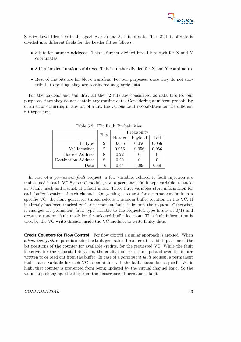
This concerns with the flow of data through links between routers and also through therouter. In this case, the datapath components are the links, VC buffers and path throughthe different components of the router. Transient errors can be SEUs and SETs. SETscan be latched and manifest as SEUs in the buffers. SEUs can also happen directly atthe buffers. Permanent faults can be stuck-at faults in case of buffers, and broken wires,shorted wires or wires that are stuck to a voltage level. So it is convenient to think offault injection of datapath components in this layer in terms of two different types oflocations: wires and buffers. Each wire should have a saboteur type of fault injectorwhich modifies the signal going to the destination. One saboteur component per linkshould be able to simulate faults in the wire between the output port to the input port.In the present case, the saboteur component has been associated with the input side,i.e. the input ports of each router. In the case of the VC buffers, each VC (multiple VCsassociated with each wire) can have some mutant logic in the code which would modifythe current contents of its own buffer.
Depending on which bit position the fault occurs in the VC buffer or link, and alsothe type of flit, it can have different effects. It could change the flit payload (i.e. thedata contained in the flit), the destination address or even modify the type of flit it hasbeen designated as. This also depends on the type of the original flit, since different flittypes will have different flit formats. For example, a Body flit will not have destinationaddress information.
The control logic components in this layer are the flow control logic. Although anSEU is a transient fault, in this case it can affect router operation permanently. Thisis because when a transient fault changes the credit counter, this value is used for allfuture router operations till the router or NoC is reset, making the fault effect essentiallypermanent. It can lead to less flits being sent than capacity, or router stalls. Permanentfaults can manifest themselves as stuck-at faults in the credit counter, or a credit counterwhich fails to update. In this fault injection framework, permanent faults have beenimplemented as a counter which stops updating.
5.1.2. Network Layer
This is concerned with the correct routing of flits along the path from source to des-tination. Concerned physical locations, which are solely control logic components, arethe RCUs, crossbar and VC allocation unit. The way faults in these components affectthe packet transmission differs, and is also different in transient or permanent faults.Since all the faults occur in the control logic inside functional components, they are bestsimulated using mutants.
RCU In case of the RCU, when a transient fault occurs, it will direct the whole packetto a wrong output, since only the head flit is involved in routing computation. Restof the flits will follow the same direction. In case of permanent faults, the situation issimilar; only all the packets will be sent to a single output port. It is important to note
36 CONFIDENTIAL
that since the RCU is before the VA, the flits will all be routed through correct VCs andhence there won’t be any overlap of flits from different packets.
Crossbar Unlike the RCU, the crossbar works on the flit level. It sends each flit to anoutput port based on the port select signal it has received. Hence in case of the crossbar,when a transient fault occurs, a single flit from an input port may be redirected to awrong output port. Since this is at flit level, some flits of a packet maybe sent elsewherethan the rest, leading to flit loss and loss of packet integrity, which is harder to recoverfrom. In case of permanent faults, this problem is not apparent since all flits are directedto the same port. However, since the crossbar is after the VA, on occurrence of faults,flits from different VCs can overlap and be ejected out of order from the output port(s).
VC Allocator Faults can occur in two different ways in the VC Allocator. The VCallocator may allocate random VCs to a flit in temporary fault mode, or send all flitsin the same VC, or lose all flits, in permanent fault mode. Also,the priority orderingof packets might be disrupted due to a fault. So, a packet which was supposed to besent first might be kept waiting for other packets till the fault condition is resolved, intemporary fault mode, or permanently kept waiting in permanent fault mode.
Faults in the network layer can also be due to unresolved errors from the data linklayers like address modification, or type of flit modification.The data link layer errorsdon’t seem to be solvable by this layer and would be propagated to the transport layer,with the exception of stochastic methods (flooding, random walk) [47] where the correctinformation is available in a redundant packet.
5.1.3. Transport Layer
This is concerned with end to end transmission of packets (collection of flits) from sourcenode to destination node. In this case it covers the packet entering the network interfacefrom the source node, traveling through routers to the destination router and exitingthrough the network interface into the destination node.
Faults can happen due to unresolved errors from the lower layers, i.e. package corrup-tion (from Data Link Layer) or package loss (from Network layer). Besides this, faultscan occur directly at the transport layer in terms of data corruption and package loss atthe network interfaces at the source and/or destination nodes. Flits might be lost, thewhole package might be lost, data or address might be corrupted at one of the networkinterfaces. Like all other cases, this can be temporary or permanent. In summary, theerrors of the transport layer can be emulated in similar way to the faults in the buffersof the data link layer.
A summary of how faults in the different physical locations in a router affect the NoCin the different OSI layers is given in Table 5.1.
CONFIDENTIAL 37
Table 5.1.: Effect of faulty components on OSI layers
Component Data Link Layer Network Layer Transport Layer
Link 3 3 3
VC Buffer 3 3 3
Credit Counter 3 3 3
RCU 7 3 3
Crossbar 7 3 3
VC Allocator 7 3 3
5.2. Fault Injection & Diagnostics in the NoC Explorer
As discussed previously, the optimum way of injecting faults in a network on chip is todivide the injection into specific physical locations, while keeping in view the OSI layersassociated with each. The NoC Explorer has thus been extended with fault injectioncapabilities using the same idea. The following sections first describe the frameworkand fault injection concepts in general and then go on to describe the fault generationmechanisms in the different layers.
5.2.1. Framework
In brief, a fault injection manager has been designed which is responsible for generatingrandom faults at different locations of the NoC. The data regarding the faults to begenerated is sent to each router in the NoC through signals from the manager. Therouter components then appropriately generate the requested faults. A record of faultrequests are kept by the fault injection manager in a separate CSV file, viz. faultReq.csv.An important observation is that all fault requests may not manifest as a fault in theflit/packet delivery. Hence a separate record of the fault generation requests is beneficial.I addition, the record of the packet and flit path throughout the whole simulation timewindow is stored for the analysis of effects of individual faults.
5.2.1.1. Fault Injection Manager
The fault injection manager is the central entity that is responsible for fault injection,as well as keeping record of the fault injection requests. It generates a list of faultsto be injected in every node at each clock cycle, according to a given fault probabilitydistribution. It communicates the fault generation requirement to each router through asignal to each one of them, after which the appropriate component in the router generatesa fault. The information available in the fault signal from the fault injection manager ispresented below:
Flag Indicates whether a fault needs to be generated
Component Specifies at which component in or around the router the fault would belocated. Possible locations are link, VC buffer, flow control credit counter, routing
38 CONFIDENTIAL
computation unit, crossbar, and physical link & VC allocator.
Port Specifies which port the component is associated with. This does not apply to thecrossbar since there is only one crossbar present in a router.
Channel In applicable cases, specifies which virtual channel is to be affected. This doesnot apply to links, routing computation units or the crossbar.
Duration Specifies if the fault is permanent or transient, and if temporary, the durationof the fault. A value of 0 indicates a permanent fault, while any other non-zerovalue represents the duration of the temporary fault, in nanoseconds (ns).
In terms of implementation, this information is in the form of a C++ structure, whichis passed as a SystemC signal input to the routers. To make the structure SystemC-compatible, overloaded output stream, equality and copy operators were defined. Alsofor SystemC trace generation, a friend function sc trace() was defined.
The probability with which faults are generated is a two-level process. On the firstlevel, the routers that will be affected by a fault is selected with a probability valueset by the user, using a uniform distribution. Then, for each router that is affected,the specific component that is affected is decided with equal probability from a uniformdistribution.
It should be noted that in real world scenarios, this probability distribution is nottotally realistic. Any component of the NoC can be affected, and the probability of thishappening depends on component area, complexity of the component, the technology ofsilicon used and environmental factors. This would require a more detailed level of mod-eling the circuits, fault mechanisms and the environment, and has not been attemptedin the present work. The framework could be extended in the future to support such arealistic modeling paradigm.
5.2.1.2. Routers
Fault information signals from the fault injection manager connect to the routers. Allthe applicable components in and around the router where faults may be possible receivea copy of the fault signal, which is used by them to generate appropriate faults whenrequired. However, except the crossbar and the physical link & VC allocator, all theother components have multiple instances in the router, one each for each associatedinput port. The different instances of the same component have no information regardingwhich ports they are associated with, making it impossible to generate the fault in thecorrect component.
To solve the aforementioned issue, in each router there is a fault handler component.The components with multiple instances also have a separate fault enable signal input.The fault handler basically takes in the information from the fault signal and asserts thefault enable input of the component where the fault is to be generated. On receiving afault enable signal, the respective component generates a fault based on the informationin the fault signal. The signals inside the a router, for a single input port, is shown inFigure 5.1.
CONFIDENTIAL 39
Figure 5.1.: Router with Fault Injection Components
5.2.1.3. Flit Format & Flit Update
In addition to the data already present in the NoC Explorer flit data structure, eachflit is appended with additional information about the fault, for debug and verificationpurposes. These additions are listed below:
Fault flag Indicates whether the flit had encountered a fault
Timestamp Specifies when during the simulation time it had encountered the fault
Fault location Indicates which node the flit had encountered the fault at.
Fault type Indicates whether the fault results in a data error, a routing error or any othercontrol logic error. This depends on the component where the fault is generated.
Redundant data All the flit data that can possibly be modified by a fault are replicatedas “original” data fields. These are untouched by the fault injection mechanismand can later be used to ascertain whether a fault is present, by comparing withthe current data fields.
Except for the redundant information fields, all of the aforementioned fields are up-dated when the flit encounters the effects of a fault. The redundant fields are writtenat the time of the flit creation, by the traffic generator nodes. It should be assertedthat this information is only used for verification purposes and should not used by faultdetection and mitigation techniques of the fault tolerant NoC.
5.2.1.4. Faulty Flit Data
A method of monitoring the fault status of flits as they leave the NoC is required, inorder to verify whether faults are being injected properly, and also to verify that thefaults are being detected and mitigated by the reliability measures designed into theNoC later on.
40 CONFIDENTIAL
In the NoC Explorer, the Traffic Manager is the main entity responsible for monitor-ing of the flits leaving the NoC. Hence, it has been extended to support the function.Whenever a flit arrives at the Traffic Manager, it checks its fault flag. If enabled, itwrites down all the fault-related information to a CSV file, viz. faultyFlit.csv.
Also there might be cases where a faulty flit is dropped when it arrives out of order,without an associated Header flit, and hence never reaches a network interface. TheTraffic Manager thus never encounters them. Flits are usually dropped in at the RCU.To handle these cases, the RCU has also been modified so that when it drops a flit, it alsowrites the fault-related information into the same CSV file if the fault flag is enabled.
The information from the flit that is written into the CSV file is:
• Fault type
• Fault location
• Original and current packet IDs
• Original and current Source nodes
• Original and current Destination nodes
• Exit node
5.2.1.5. Router Stalls
Faults may cause certain components of a router to fail, causing a stall due to whichpackets cannot move through the router. This can also indirectly affect traffic around therouter, stalling other routers in the process. The list of stalled routers is also recordedafter a simulation run, and stored in the routerStall.csv file.
When a router stalls, one or more flits get stuck in the router buffers. This facthas been used to find the stalled routers. The state of all VC buffers in each router ismonitored. At the end of the simulation run, if any buffer of a router is non-empty, it isconsidered to be stalled and is recorded into the CSV file.
5.2.1.6. Packet & Flit Path
A fault occurring at a specific location can trigger direct effects on flits passing throughthe concerned router as well as indirect effects on flits in nearby routers. In order toproperly study and analyze this behavior, the path taken by each flit for the wholesimulation run is stored in a file (flitPath.csv). This has been achieved by recording thedetails of every flit that enters the RCU of a router.
The information for each flit available in the file is:
• Original Packet ID
• Current Packet ID
• Current router/node
CONFIDENTIAL 41
• Current VC
• Time stamp
However, due to the huge amount of data generated because of this, an option hasbeen implemented to only record incoming head flits. This effectively makes it a packetpath recorder, and has been kept as the default option. In case a finer granularity oftraffic information is needed, for example to check whether body or tail flits are routeddifferently than head flits in case of a fault, the flit path option can be enabled from theconstants.h header file.
5.2.1.7. Faulty Packet Statistics using Python Script
A Python script called faultStats.py has been developed which aggregates all the faultyflit data and outputs the number of packets with different kinds of faults, i.e. number ofpackets with data faults, routing faults due to data errors, routing faults due to othercauses, packets with fault flag enabled but no visible effects, and missing packets. Apacket with one or more flits which are faulty is considered a faulty packet. If there aremultiple faulty flits in a single packet, the type of fault recorded is the one with the firstfaulty flit in the packet sequence.
Details of the script can be found in Appendix B.2.1. There are other Python scriptswhich have been developed for specific test scenarios, which have been discussed later inChapter 6.
5.2.2. Mechanisms
5.2.2.1. Data Link Layer
Fault injection in the data link layer is the most involved since it is closest to thecomponent level. The various components pertaining to the data link layer are thephysical links, virtual channel buffers, ACK signals, and credit counters for flow control.Fault injection for transient and permanent faults for these components are implementeddifferently, as explained below.
Virtual Channel Buffers A fault generator thread has been implemented inside thevirtual channel SystemC module, which acts as a mutant for the virtual channel buffers.It is triggered by positive edges of the fault enable signal, which is driven by the faulthandler component. When a transient fault request is received, it selects a random bufferlocation in the requested VC buffer, using a uniform distribution, and creates a bit flipat a random bit position of one of the fields of the flit, also using a uniform distribution.This happens for all flits that may pass into that buffer location while the fault is activefor the requested duration. How a field is chosen depends on the flit format for the NoCbeing considered.
For the NoC of Recore Systems, a flit is 36 bits long. Each flit, of any type, has 2 bitsfor flit type (Empty/Idle, Header, Payload, Tail), 2 bits for VC identifier (also called
42 CONFIDENTIAL
Service Level Identifier in the specific case) and 32 bits of data. This 32 bits of data isdivided into different fields for the header flit as follows:
• 8 bits for source address. This is further divided into 4 bits each for X and Ycoordinates.
• 8 bits for destination address. This is further divided for X and Y coordinates.
• Rest of the bits are for block transfers. For our purposes, since they do not con-tribute to routing, they are considered as generic data.
For the payload and tail flits, all the 32 bits are considered as data bits for ourpurposes, since they do not contain any routing data. Considering a uniform probabilityof an error occurring in any bit of a flit, the various fault probabilities for the differentflit types are:
In case of a permanent fault request, a few variables related to fault injection aremaintained in each VC SystemC module, viz. a permanent fault type variable, a stuck-at-0 fault mask and a stuck-at-1 fault mask. These three variables store information foreach buffer location of each channel. On getting a request for a permanent fault in aspecific VC, the fault generator thread selects a random buffer location in the VC. Ifit already has been marked with a permanent fault, it ignores the request. Otherwise,it changes the permanent fault type variable to the requested type (stuck at 0/1) andcreates a random fault mask for the selected buffer location. This fault information isused by the VC write thread, inside the VC module, to write faulty data.
Credit Counters for Flow Control For flow control a similar approach is applied. Whena transient fault request is made, the fault generator thread creates a bit flip at one of thebit positions of the counter for available credits, for the requested VC. While the faultis active, for the requested duration, the credit counter is not updated even if flits arewritten to or read out from the buffer. In case of a permanent fault request, a permanentfault status variable for each VC is maintained. If the fault status for a specific VC ishigh, that counter is prevented from being updated by the virtual channel logic. So thevalue stop changing, starting from the occurrence of permanent fault.
CONFIDENTIAL 43
Physical Links Faults in the physical links are implemented using a saboteur compo-nent, between each input port and RCU. A thread monitors the fault data and faultenable signals and maintains a fault mask and a fault state variable. In case of perma-nent faults, it generates a random mask and asserts the fault state variable true, if thefault state variable was not already true. In case of transient faults, if the fault statevariable is not already true, it changes the fault mask and asserts the fault state variableto be true for the duration requested.
Figure 5.2.: Fault generation in physical links
The saboteur component monitors the fault state variable. It directly passes on thedata from input to output when the fault state variable is false. When it is true, thecomponent modifies the data and outputs it to the RCU. The data is modified with thesame probabilities as discussed in the case of VC buffers. This concept has been shownin Figure 5.2.
5.2.2.2. Network Layer
The components relating to the Network Layer are the RCU, crossbar and the physicallink & VC allocator. In the present work, fault injection has been added to all thesethree components. The implementation follows a similar pattern as in the previouscases. A separate thread (fault thread()) keeps track of the fault signal, and maintainsa fault state variable which is monitored by other functions in the component in orderto generate the fault.
RCU Since there are as many RCUs as there are router ports, the fault enable signal issent to the correct RCU by the fault handler, which is monitored by the fault thread().If the fault state variable is not already true, in case of a permanent fault a randomfaulty output direction is assigned and the fault state variable is made permanentlytrue. Hence any packet that passes through is given the same output direction. In caseof transient faults the same is done only for the duration specified, after which the faultstate variable is returned to false. Next time, if a transient fault occurs in the sameRCU, the faulty output direction might be different from the previous fault case.
44 CONFIDENTIAL
Crossbar Since there is a single crossbar in a router, there is no need for the faulthandler. The fault signal from the fault injection manager is directly monitored by thefault thread() inside the crossbar module. If the fault state variable is not already true,in case of a permanent fault a random faulty output port is assigned and the fault statevariable is made permanently true. Hence all flits which pass are sent into the sameoutput port.In case of transient faults the same is done only for the duration specified,after which the fault state variable is returned to false. Next time, if a transient faultoccurs in the same RCU, the faulty output port might be different from the previousfault case.
It must be asserted that even though the mechanisms are similar in the crossbar andRCU, they work in different levels of granularity. The RCU fixes a direction for thewhole packet, when the head flit arrives, and so the whole of the faulty packet is sentto the wrong direction. However, the crossbar works on a flit-to-flit basis. Hence a fewflits of the packet can sent to the wrong output port while the rest goes to the correctoutput port, depending on when the fault was injected. It can therefore also lead topacket integrity errors.
Physical Link & VC Allocator Since there is a single physical link & VC allocator ineach router, the fault signal from the fault injection manager is directly monitored by thefault thread() inside the module. Out of the two fault possibilities mentioned in Section5.1.2, fault injection in the input port ordering has been implemented. The PhysicalLink & VC Allocator scans the input ports in priority order (port 0 to port N) or inround robin order, and sends the packets to the destined output ports. If the fault statevariable is not already true, in case of a permanent fault a random input port is assignedand the fault state variable is made permanently true. Hence only packets from thatinput port would be sent to output ports, rest would be kept in waiting permanently.In case of transient faults the same is done only for the duration specified, after whichthe fault state variable is returned to false. Next time, if a transient fault occurs in thesame RCU, the input port chosen might be different from the previous fault case.
5.2.2.3. Transport Layer
In the case of Transport Layer, no separate fault injection methods have been imple-mented. Unresolved errors in the lower layers which can trigger transport layer errorslike packet loss, out of order arrival can be studied, for the purposes of detection andmitigation techniques.
CONFIDENTIAL 45
Chapter 6.
Simulation Results
In this chapter the fault injection framework is tested by simulating various NoC, trafficand fault conditions. At first, the effect of a single fault in the NoC is evaluated andanalyzed. This helps us to look at direct as well as indirect effects that a fault can causeto the NoC. Then the framework is compared to literature under different conditions, toascertain whether the effects of faults follow the same trend, as a means to qualitativelyvalidate the fault injection functionality. Finally a performance profiling of the NoCExplorer with fault injection enabled is done, and compared with the framework disabled,in order to realize the overhead caused due to the fault injection framework.
6.1. Single Fault Tests
This section serves to provide an idea of how a single fault at a component can affect theoperation of the NoC. All the six components where fault injection is possible, i.e. theVC buffers, links, flow control, RCU, crossbar and the physical link and VC allocator,have been tested separately.
In each simulation run, a single component of one random router in the NoC hasbeen injected with a fault. 30 such simulation runs have been done for a single type ofcomponent. This has been repeated for all six components. So, in total, 30 * 6 = 180simulation runs have been performed.
The parameters that have been used in these simulations are:
Without any fault occurring, at the set traffic and simulation conditions, 31250 pack-ets are transmitted through the NoC. This number can be less in cases in which one
CONFIDENTIAL
or a number of routers are stalled due to faults, leading to their inability to acceptpacket requests from the traffic generator nodes. In the single fault testing, a system-atic approach has been followed. For each component type, the data regarding thesingle fault generated in the NoC and the details of the number of packets affected bythe fault in different ways, for all 30 simulation runs, are aggregated into a single file.Moreover, for the cases where there are faulty packets and/or missing packets, the filesrelated to the original intended NoC traffic pattern (trafficPattern.csv), missing packets(checkPacket.report), the faulty flit faultyFlit.csv) and the path taken by the packets(flitPath.csv) are recorded. From these files, the faulty and missing flits are found outand, by looking at the path taken and other details (explained later), the effect of thesefaults in the NoC can be deduced.
In order to understand the node positions and the paths taken by the packets, a layoutof the 5x5 NoC with node numbers is provided in Figure 6.1.
0 1 2 3 4
5 6 7 8 9
10 11 12 13 14
15 16 17 18 19
20 21 22 23 24
Figure 6.1.: NoC Layout for Single Fault Testing
In each of the single fault test discussions, the results of the 30 injections are given inthe form of a table. Each table contains some or all of the following information:
• Time stamp of fault occurrence (in ns)
• Faulty Router
• Component of the router where fault has occurred
• Port which the component is associated to (not applicable for the crossbar or thephysical link & VC allocator)
• VC (only applicable for the case of faults in VCs)
• Total detected faulty packets (i.e. packets received with one of the flits having afault flag enabled)
• Number of these faulty packets which have data faults
• Number of packets which have routing faults due to data errors
• Number of packets which have routing faults due to other causes
48 CONFIDENTIAL
• Number of packets which do not show any effect of a fault, even though they haveflit(s) fault flags enabled.
• Missing packets: these may or may not have faulty packets, but are definitelymissing
6.1.1. Faults in Links
Table 6.1.: Link Fault Statistics
No. TimeStamp(ns)
FaultyRouter
Comp-onent
Port Duration(ns)
TotalFaultyPackets
DataFaults
RoutingFaultsdue toData
OtherRout-ingFaults
NoMani-festedFaults
MissingPackets
1 9 10 Link NI 2 0 0 0 0 0 0
2 303 6 Link Port 2 14 0 0 0 0 0 0
3 203 19 Link NI 20 0 0 0 0 0 0
4 21 13 Link Port 2 11 0 0 0 0 0 0
5 169 18 Link Port 2 10 0 0 0 0 0 0
6 787 6 Link Port 3 16 0 0 0 0 0 0
7 647 6 Link NI 17 0 0 0 0 0 0
8 21 22 Link Port 3 5 0 0 0 0 0 0
9 125 20 Link Port 2 12 0 0 0 0 0 0
10 157 20 Link Port 3 5 0 0 0 0 0 0
11 1165 2 Link Port 1 15 0 0 0 0 0 0
12 5 17 Link Port 2 17 1 1 0 0 0 0
13 801 11 Link Port 1 18 1 1 0 0 0 0
14 11 13 Link Port 1 7 1 1 0 0 0 0
15 299 17 Link Port 2 9 0 0 0 0 0 0
16 331 18 Link Port 1 10 0 0 0 0 0 0
17 39 9 Link Port 2 14 0 0 0 0 0 0
18 275 1 Link Port 2 18 0 0 0 0 0 0
19 115 24 Link NI 1 0 0 0 0 0 0
20 281 8 Link Port 1 10 1 1 0 0 0 0
21 91 1 Link Port 2 5 1 1 0 0 0 0
22 1011 3 Link Port 2 2 0 0 0 0 0 0
23 717 23 Link Port 3 15 1 1 1 0 0 0
24 213 12 Link Port 3 11 0 0 0 0 0 0
25 287 23 Link Port 1 1 0 0 0 0 0 0
26 77 19 Link Port 1 11 1 1 0 0 0 0
27 283 7 Link Port 2 2 0 0 0 0 0 0
28 507 21 Link Port 3 9 0 0 0 0 0 0
29 149 22 Link Port 1 14 1 1 1 0 0 0
30 453 11 Link Port 3 16 0 0 0 0 0 0
The results of single fault injections into the NoC links is shown in Table 6.1. Out of 30injections, only 8 packets have been affected by the faults. This shows that most faultsdo not actually affect proper NoC operation. This is because, in order for a fault to
CONFIDENTIAL 49
affect a flit, there needs to be an active operation with a flit happening in the specificcomponent of the router, when the fault occurs. Also out of these 8 faults, all of themhave predictably created data faults, out of which only 2 data faults have resulted inrouting faults. This is because there is more probability of a bit flip occurring in thepayload area of a flit, and also because address errors can only happen in the case ofheader flits.
6.1.2. Faults in VC Buffers
Table 6.2.: VC Fault StatisticsNo. Time
Stamp(ns)
FaultyRouter
Comp-onent
Port VC Duration(ns)
TotalFaultyPackets
DataFaults
RoutingFaultsdue toData
OtherRout-ingFaults
NoMani-festedFaults
MissingPackets
1 113 7 Buffer Port 1 2 15 0 0 0 0 0 0
2 323 5 Buffer NI 0 4 0 0 0 0 0 0
3 79 12 Buffer Port 2 3 10 0 0 0 0 0 0
4 93 21 Buffer NI 0 7 0 0 0 0 0 1
5 621 17 Buffer Port 3 0 14 0 0 0 0 0 0
6 413 4 Buffer Port 3 0 11 0 0 0 0 0 0
7 465 1 Buffer Port 2 0 3 0 0 0 0 0 0
8 289 21 Buffer Port 1 2 8 0 0 0 0 0 0
9 277 24 Buffer Port 3 3 1 0 0 0 0 0 0
10 65 14 Buffer NI 1 20 0 0 0 0 0 0
11 625 22 Buffer NI 2 13 0 0 0 0 0 0
12 195 18 Buffer Port 1 0 16 0 0 0 0 0 0
13 217 23 Buffer Port 2 3 10 0 0 0 0 0 0
14 865 22 Buffer NI 2 6 0 0 0 0 0 0
15 23 24 Buffer NI 3 11 0 0 0 0 0 0
16 633 4 Buffer NI 0 11 0 0 0 0 0 0
17 215 9 Buffer Port 3 3 10 0 0 0 0 0 0
18 111 22 Buffer Port 2 2 17 0 0 0 0 0 0
19 817 12 Buffer Port 1 1 5 0 0 0 0 0 0
20 1179 19 Buffer Port 2 3 19 0 0 0 0 0 0
21 411 13 Buffer Port 2 0 18 1 1 0 0 0 0
22 51 8 Buffer Port 1 2 1 0 0 0 0 0 0
23 1607 18 Buffer Port 1 3 4 0 0 0 0 0 0
24 1613 21 Buffer Port 2 2 3 0 0 0 0 0 0
25 1061 7 Buffer Port 1 2 4 0 0 0 0 0 0
26 203 17 Buffer Port 3 3 6 0 0 0 0 0 0
27 709 13 Buffer Port 1 1 8 0 0 0 0 0 0
28 417 9 Buffer Port 3 3 12 0 0 0 0 0 0
29 41 17 Buffer Port 1 1 19 0 0 0 0 0 0
30 1317 12 Buffer Port 3 2 7 0 0 0 0 0 0
The results of the single fault injections into VC buffers is shown in Table 6.2. Out of the30 simulation runs, one has a case of a data corruption, and one has a missing packet.
The packet with data corruption is in simulation run no. 21, with a packet ID of2100006. It has a payload error, and so no routing errors have occurred. The missing
50 CONFIDENTIAL
packet is in simulation run no. 4, with a packetID of 2001250. Its source and destinationnodes are 20 and 8, respectively. Looking at the path followed by the packet (usingflitPath.csv data): 20→ 21→ 22→ 23→ 18→ 13 (Figure 6.2), shows that the packethas followed the correct path according to XY routing. However the head flit has reachednode 13 at 99997 ns. Since the simulation time window is 100000 ns, it did not havetime to reach the final destination node. This is just due to simulation time chosen andother random traffic factors and not related to faults.
2001250
0 1 2 3 4
5 6 7 8 9
10 11 12 13 14
15 16 17 18 19
20 21 22 23 24
Figure 6.2.: Packet path for VC buffer test
6.1.3. Faults in Flow Control
The results of the single fault injection in the flow control credit counters of the routersis given in Table 6.3. There are a number of missing packets in almost all the 30 cases,amounting to a total of 478 missing packets. However, there are no detected faulty flitsin any of the cases. This is due to a discrepancy between the counter value and theactual number of free buffer slots in the buffer, which is maintained separately by thebuffer read and write logic. This can be explained as follows: the VC buffers in this casehave a depth of four flits, which is equal to one packet. Since the maximum value of thecredit counter would be equal to the buffer depth of 4 (2 bits), any fault can only causethe counter to be of some value from 0 to 4. Two cases can occur:
• If the fault changes the credit counter to a value which is less than the originalvalue (i.e. there are more slots empty than shown by the counter), then no flitscan get stored in the buffer after a point, even if it is not full. The next packetcoming in will thus be partially stored, stalling the associated routers.
• If the fault changes the credit counter to a value which is more than the originalvalue (i.e. there are less slots empty than shown by the counter), even though theupstream router tries to transmit the packet, the FIFO buffer logic inside the VCwill prevent anything from being written after it is full. The packet will be thuspartially transmitted, stalling the associated routers.
CONFIDENTIAL 51
It is to be noted that this situation is aggravated since the buffer depth is equal to thepacket size, due to which any kind of fault completely prevents the transmission of thepacket. If the buffer depth were greater than the packet size, there would be a possibilityof packet transmission even in the presence of a fault, albeit at a lower effective (usable)buffer size.
Table 6.3.: Flow Control Fault StatisticsNo. Time
Stamp(ns)
FaultyRouter
Comp-onent
Port VC Duration(ns)
TotalFaultyPackets
DataFaults
RoutingFaultsdue toData
OtherRout-ingFaults
NoMani-festedFaults
MissingPack-ets
1 119 2 Flow Ctrl. Port 3 2 15 0 0 0 0 0 5
2 137 9 Flow Ctrl. Port 3 0 3 0 0 0 0 0 0
3 631 13 Flow Ctrl. NI 2 14 0 0 0 0 0 29
4 123 0 Flow Ctrl. Port 2 0 3 0 0 0 0 0 59
5 569 15 Flow Ctrl. Port 2 2 11 0 0 0 0 0 14
6 469 9 Flow Ctrl. Port 3 1 16 0 0 0 0 0 0
7 25 11 Flow Ctrl. NI 1 16 0 0 0 0 0 29
8 321 3 Flow Ctrl. Port 2 1 1 0 0 0 0 0 59
9 999 15 Flow Ctrl. Port 2 0 5 0 0 0 0 0 14
10 41 12 Flow Ctrl. NI 1 12 0 0 0 0 0 29
11 15 24 Flow Ctrl. NI 1 6 0 0 0 0 0 0
12 223 12 Flow Ctrl. Port 2 3 1 0 0 0 0 0 29
13 453 6 Flow Ctrl. Port 3 1 3 0 0 0 0 0 8
14 639 15 Flow Ctrl. Port 3 0 3 0 0 0 0 0 11
15 311 21 Flow Ctrl. Port 1 1 11 0 0 0 0 0 2
16 175 2 Flow Ctrl. Port 3 3 10 0 0 0 0 0 5
17 281 24 Flow Ctrl. NI 1 3 0 0 0 0 0 0
18 53 2 Flow Ctrl. NI 1 16 0 0 0 0 0 0
19 25 11 Flow Ctrl. Port 3 0 13 0 0 0 0 0 8
20 125 2 Flow Ctrl. NI 0 4 0 0 0 0 0 0
21 1523 7 Flow Ctrl. Port 2 2 13 0 0 0 0 0 44
22 269 14 Flow Ctrl. Port 2 1 11 0 0 0 0 0 29
23 51 22 Flow Ctrl. Port 3 0 5 0 0 0 0 0 5
24 117 4 Flow Ctrl. NI 2 17 0 0 0 0 0 0
25 199 5 Flow Ctrl. Port 3 1 17 0 0 0 0 0 11
26 173 19 Flow Ctrl. NI 1 17 0 0 0 0 0 44
27 385 9 Flow Ctrl. NI 0 6 0 0 0 0 0 14
28 105 14 Flow Ctrl. Port 1 0 16 0 0 0 0 0 11
29 293 12 Flow Ctrl. Port 3 3 17 0 0 0 0 0 5
30 113 5 Flow Ctrl. NI 0 2 0 0 0 0 0 14
In order to better understand how the packets go missing, the case of simulation runnumber 1, with 5 missing packets, has been considered. The fault has occurred in port 3of router 2, inside VC 2. The fault timestamp is 119 ns. Going in the order of injectiontime, the missing packet has with ID 400003, has source and destination nodes 4 and 17,respectively. Looking at the path taken by the packet: 4→ 3 along VC 2, it can be seenthat the packet stalls at 3. Since the credit counter of VC 2 in router 2 has a fault atthe input port from 4→ 3 (port 3), the packet cannot reach router 2 and is stalled. It isstored in VC 2 of router 3 and hence has blocked VC 2 of the 4→ 3 input port of router
52 CONFIDENTIAL
3. The next packet, with ID 400007, with source and destination nodes 4 and 16, triesto move into router 3 through VC 2, and gets stalled in router 4 because of the blockedVC in router 3. The packet is now stored in the input port of the router connectedto the Master NI, blocking VC 2 of that input port. The packet with ID 300011, hassource and destination nodes 3 and 7, respectively. Also following VC 2, it gets stalledat router 3 because of the faulty credit counter of router 2. It then blocks VC 2 of theinput port connected to the Master NI. The packet with ID 400011 cannot even enterrouter 4 because of the blocked VC 2 of input port from the Master NI, being blockedby packet 400007. The packet with ID 300015, with source and destination nodes 3 and2, shares a similar fate, being blocked due to packet 300011. This has been shown inFigure 6.3.
Figure 6.3.: Packet path for flow control test
6.1.4. Faults in RCUs
The results of the RCU single fault injection is given in Table 6.4. There are 3 packetsthat have been affected by faults, all of which seem to have had no manifested effect.This means that these packets have reached their correct destination in spite of thefaults. There are also two cases of missing packets.
The packet with packetID 1100004 in simulation run no. 12 has the source at node11 and destination at node 7. The fault location is also node 7. From the path followedby the packet: 11 → 12 → 7 → 6 → 7 (see Figure 6.4), it can be seen that the packetreaches the faulty destination node, is sent back to node 6. It is then sent by node 6back to its intended destination following the XY routing protocol.
The packet with packetID 8 in simulation run no. 23 has the source at node 0 anddestination at node 11. The fault location is node 6. From the path followed by thepacket: 0→ 1→ 6→ 7→ 6→ 11 (Figure 6.4), it can be seen that at node 6, the packetis incorrectly sent to node 7 due to the fault. However, following XY routing protocol,node 7 sends it back to node 6, which is then sent correctly to node 11 since node 6RCU is not faulty anymore.
CONFIDENTIAL 53
Table 6.4.: RCU Fault Statistics
No. TimeStamp(ns)
FaultyRouter
Comp-onent
Port Duration(ns)
TotalFaultyPackets
DataFaults
RoutingFaultsdue toData
OtherRout-ingFaults
NoMani-festedFaults
MissingPackets
1 75 21 RCU NI 4 0 0 0 0 0 0
2 181 9 RCU Port 3 8 0 0 0 0 0 0
3 9 2 RCU NI 10 0 0 0 0 0 0
4 47 14 RCU Port 3 6 0 0 0 0 0 0
5 583 15 RCU Port 3 9 0 0 0 0 0 0
6 597 3 RCU Port 1 19 0 0 0 0 0 2
7 729 3 RCU Port 1 5 0 0 0 0 0 0
8 249 13 RCU Port 3 20 0 0 0 0 0 0
9 331 19 RCU NI 6 0 0 0 0 0 0
10 195 22 RCU Port 1 13 0 0 0 0 0 0
11 229 5 RCU Port 3 4 0 0 0 0 0 0
12 235 7 RCU Port 2 16 1 0 0 0 1 0
13 345 9 RCU NI 17 0 0 0 0 0 0
14 271 3 RCU NI 19 0 0 0 0 0 0
15 629 1 RCU Port 1 7 0 0 0 0 0 0
16 651 0 RCU Port 2 15 0 0 0 0 0 0
17 89 14 RCU NI 8 0 0 0 0 0 1
18 211 9 RCU Port 2 20 0 0 0 0 0 0
19 111 6 RCU NI 16 0 0 0 0 0 0
20 289 5 RCU Port 1 10 0 0 0 0 0 0
21 9 8 RCU Port 2 5 0 0 0 0 0 0
22 227 6 RCU Port 2 5 0 0 0 0 0 0
23 563 6 RCU NI 12 1 0 0 0 1 0
24 987 0 RCU Port 1 3 0 0 0 0 0 0
25 663 19 RCU NI 8 0 0 0 0 0 0
26 61 3 RCU Port 2 12 0 0 0 0 0 0
27 201 2 RCU Port 3 15 0 0 0 0 0 0
28 93 13 RCU NI 20 1 0 0 0 1 0
29 519 21 RCU Port 1 9 0 0 0 0 0 0
30 275 8 RCU Port 3 2 0 0 0 0 0 0
The packet with packetID 2 in simulation run no. 28 has its source at node 0 anddestination at node 18. The fault has occurred in node 13. Looking at the path followedby the packet: 0→ 1→ 2→ 3→ 8→ 13→ 8→ 13→ 18 (Figure 6.4), we see that thefault has pushed the packet back to the previous node, and hence following XY routingalgorithm, it has moved again to node 13 and completed its intended path to reach node18.
Hence, in general, a fault in the RCU has a less detrimental effect on the routing, sincethe XY routing protocol takes care of small changes in the path caused by the faultyRCU. The only effect it has in this case is an increase in latency. However, one case hasnot been seen in the 30 iterations: the fault in the RCU can make the output port to bethe slave NI instead of any of the other router directions. In that case the packet will
54 CONFIDENTIAL
leave the NoC from the faulty node and hence not reach its intended destination.
Besides these, there also are cases of missing packets. Considering the first case,of simulation no. 6, we see that the missing packets have packet IDs of 1601250 and1501250. Packet 1501250 has source and destination nodes to be 15 and 14, respectively.Packet 1601250 has source node and destination node to be 16 and 8, respectively. Fromthe flit path data, we see that in both cases the head flit reaches the intended destinationat 99997 ns. Hence this just means that all the flits of the packet were unable to exit theNoC within the simulation time window. The case for simulation run no. 17 is similar.
1100004 (Simulation 12) 8 (Simulation 23)
2 (Simulation 28)
0 1 2 3 4
5 6 7 8 9
10 11 12 13 14
15 16 17 18 19
20 21 22 23 24
Figure 6.4.: Packet paths for RCU test
6.1.5. Faults in Crossbars
The results of single fault injections in crossbars is given in Table 6.5. Out of the 30runs, 10 have faulty packets, out of which 4 have been affected by routing faults, whilethe other 6 have no manifested faults. However in each of these cases, and also incases where there are no faulty packets observed, there are numerous missing packets,amounting to 2842. Since it is too cumbersome to cover all the cases separately, a fewrepresentative cases will be considered: no faulty packets but missing packets present,faulty packets with routing errors along with missing packets, faulty packets with nomanifested faults but with missing packets, and faulty flits with no manifested faultsand no missing packets.
6.1.5.1. No faulty packets, Missing packets
Considering the case of simulation run no. 6, with 313 missing flits, the fault locationis router 0. Looking at the missing packets in increasing order of starting time, the firstflit has a packetID of 700011 with source and destination nodes 7 and 0 respectively.According to the flit path, the head flit goes through: 7 → 6 → 5 → 0 (Figure 6.5a),and is stored in VC 2 at router 0. Hence the head flit has reached the destination, at813 ns. The fault occurs at 815 ns, for 8 ns. Hence, the head flit has been sent to arandom incorrect port. Since the flit path ends at router 0, it can be inferred that the
CONFIDENTIAL 55
Table 6.5.: Crossbar Fault Statistics
No. TimeStamp(ns)
FaultyRouter
Component Duration(ns)
TotalFaultyPackets
DataFaults
RoutingFaultsdue toData
OtherRout-ingFaults
NoMani-festedFaults
MissingPackets
1 1251 10 Crossbar 18 0 0 0 0 0 0
2 373 7 Crossbar 19 0 0 0 0 0 0
3 787 20 Crossbar 5 0 0 0 0 0 0
4 443 14 Crossbar 18 0 0 0 0 0 0
5 607 4 Crossbar 2 0 0 0 0 0 0
6 815 0 Crossbar 8 0 0 0 0 0 313
7 833 8 Crossbar 10 1 0 0 1 0 321
8 869 12 Crossbar 16 1 0 0 0 1 0
9 719 10 Crossbar 14 1 0 0 0 1 349
10 1175 7 Crossbar 14 0 0 0 0 0 0
11 135 1 Crossbar 20 0 0 0 0 0 0
12 61 10 Crossbar 20 0 0 0 0 0 0
13 253 7 Crossbar 16 1 0 0 1 0 349
14 125 20 Crossbar 20 0 0 0 0 0 312
15 535 3 Crossbar 17 0 0 0 0 0 0
16 285 17 Crossbar 6 0 0 0 0 0 0
17 1923 9 Crossbar 1 1 0 0 0 1 316
18 1145 13 Crossbar 11 0 0 0 0 0 192
19 131 3 Crossbar 6 0 0 0 0 0 0
20 1233 2 Crossbar 12 1 0 0 0 1 320
21 405 6 Crossbar 17 2 0 0 1 1 48
22 57 19 Crossbar 9 0 0 0 0 0 0
23 703 10 Crossbar 6 0 0 0 0 0 0
24 297 22 Crossbar 3 0 0 0 0 0 0
25 183 7 Crossbar 15 0 0 0 0 0 0
26 139 11 Crossbar 5 0 0 0 0 0 0
27 583 3 Crossbar 15 1 0 0 0 1 322
28 339 14 Crossbar 2 1 0 0 1 0 0
29 231 9 Crossbar 3 0 0 0 0 0 0
30 137 18 Crossbar 12 0 0 0 0 0 0
56 CONFIDENTIAL
head flit was not sent to any of the neighboring routers, but attempted to be sent tothe unconnected port of router 0 which is an edge router. Due to the absence of controlsignals from the unconnected port, the Physical Layer and VC Allocator is kept busywaiting, effectively stalling the router for the specific input port (5→ 0). Also, since thepacket size is 4 flits, the rest of the 3 flits are still stored in VC 2.
Now considering packet 800011 which is supposed to move from node 8 to 0, the pathtaken is: 8 → 7 → 6 → 5 → 0 (Figure 6.5a), with the final VC being 2. Hence, it ispartially stored in the non-empty VC 2, the rest of its flits being stalled in router 5.Since the flits of packet 700011 are already present and stalled, it cannot even reach thePhysical Link and VC Allocator. On the other hand the buffer for VC 2 is filled up, andit will be unable to accept more flits.
Packet 200014, from node 2 to 0, ends with being stored at VC 1. Since the PhysicalLayer and VC Allocator is already stalled, it fails to reach the Slave NI, even thoughthere is no fault occurring at the time. Packet 700014, supposed to move from node 7to 0, moves along 7 → 6 → 5 (Figure 6.5a) in VC 1, and gets stalled at router 5 sincethat specific port from 5→ 0 is blocked with flits from packet 800011. This also meansthe VC used by packet 700014 (VC 1) at that input port (6→ 5) is full.
For the case of packet with ID 800014, which is supposed to move from node 8 to node15, it moves along 8 → 7 → 6 (Figure 6.5a) in VC 1 and gets stalled before enteringrouter 5 because of VC 1 buffer being full.
In this way a chain reaction or a domino effect occurs, and gradually many neighboringrouters get stalled in some or all ports, leading to so many missed packets. It is to benoted that in this test, the VC allocation scheme has been set to Master NI, whichmeans that the VC to be used by a packet is fixed by the Master NI and cannot bechanged in its path. So, in this case, even if other VCs in a router are free, the packetis stalled if its assigned VC is blocked in the router. Thus is can be surmised that if theVC allocation scheme were dynamic instead of being fixed at the NI, there could be lesscases of missed packets since packets could use unblocked VCs while moving throughintermediate routers.
6.1.5.2. Faulty packets with routing errors, Missing packets
Considering simulation run no. 7, with 1 detected faulty packet with routing error and321 missing packets, the fault occurs at 833 ns, in router 8. Since the router is not atany edge of the NoC, the previous problem of flits getting lost at the NoC boundary isnot possible.
First, we analyze the detected faulty packet since it is the first to be affected bythe fault. The packet ID is 100011, and source and destination nodes are 1 and 8,respectively. Tracing the path taken: 1 → 2 → 3 → 8 (Figure 6.5b) through VC 2, itcan be seen that the head flit successfully reaches the destination. However, from thefaulty flit data, it is observed that the tail flit reaches node 8, but instead of being sentinto Slave NI, it has been sent into router 7. Since it is not a head flit, it is discardedby the router. Also, since the Physical Layer and VC Allocator does not receive anyacknowledgment of the successful transmission of the tail flit, that specific input port
CONFIDENTIAL 57
(a) No Faulty Packets, Missing Packets
100011 11 121500012
0 1 2 3 4
5 6 7 8 9
10 11 12 13 14
15 16 17 18 19
20 21 22 23 24
(b) Faulty Packets with Routing Errors, Miss-ing Packets
500010600010
0 1 2 3 4
5 6 7 8 9
10 11 12 13 14
15 16 17 18 19
20 21 22 23 24
(c) Faulty Packets with No Manifested Faults,Missing Packets
(d) Faulty Packets with No Manifested Faults,No Missing Packets
Figure 6.5.: Packet paths for Crossbars
(3→ 8) allocation is not freed and the router is stalled for that input port. Even thougha packet can enter through that port and get stored in the VC, it cannot pass into anyoutput port.
Among the rest of the missing flits, the packet with ID 11 is supposed to move fromnode 0 to 8. Looking at its path: 0 → 1 → 2 → 3 → 8 (Figure 6.5b) through VC 2, itcan be seen that it has followed the right path and has entered the destination router.However, due to the stalled VC allocator, it cannot reach the Slave NI, and hence isstuck in VC 2, which also means that VC 2 is blocked for any more packets trying toenter.
The next packet with ID 12 has a similar problem. Originally supposed to go fromnode 0 to node 23, it gets stuck at router 8 due to the physical layer and VC allocator,and blocks VC 3 of that input port. For the next packet with ID 1500012, the source
58 CONFIDENTIAL
and destination nodes are 15 and 3, respectively. Looking at the path followed: 15 →16 → 17 → 18 → 13 → 8 (Figure 6.5b) through VC 3, it gets stuck at router 8 for thesame reason, also blocking VC 3 of the input port (13→ 8).
Hence we can conclude that similar to the previous case, there is a chain reaction,leading to the loss of so many packets.
6.1.5.3. Faulty packets with no manifested faults, Missing packets
Considering simulation run no. 9, with 1 detected faulty packet with no manifested errorand 349 missing packets, the fault occurs at 719 ns, in router 10. This router is also atthe edge of the NoC and hence can have flits/packets leaving the NoC.
Looking at the detected faulty packet with ID 1000010, it is seen that two of the flitsof the packet are affected by the faults, but have reached the correct destination node,17. It can be concluded that the direction imposed by the fault in the crossbar was thesame as that required by the flits to reach the correct router, i.e. towards router 15.
The first missing packet has an ID of 500010, with source and destination being nodes5 and 10. It reaches the destination node 10 at 725 ns, when the fault is still active.At the destination node 10, instead of being sent to the Slave NI, it is sent to router 15(Figure 6.5c). However, it can be concluded that by the time the tail flit has reached,the fault is deactivated, and hence the tail flit is sent to the Slave NI. Without a headflit, this is rejected and the physical link and VC allocator is stalled.
For the next missing packet with an ID of 600010, the source and destination arenodes 6 and 20 respectively. It goes through the following path: 6 → 5 → 10 (Figure6.5c) and gets stuck at 10 because of the stalled physical link and VC allocator in therouter.
The general trend continues like the previous two cases, leading to the rest of themissing packets.
6.1.5.4. Faulty packets with no manifested faults, No missing packets
In the simulation run no. 8, there is 1 detected faulty packet with no manifested errorand no missing flits. The fault occurs at 869 ns, in router 12. This case is relativelysimple to understand.
The detected flit has an ID of 1200012, with source and destination nodes 12 and21, respectively. Looking at the path: 12 → 11 → 16 → 21 (Figure 6.5d), it can beconcluded that the fault-imposed direction is the same as the required direction, leadingto the successful transmission of the flit.
6.1.6. Faults in Physical Link and VC Allocator
The results of single fault injections in physical link and VC allocator is given in Table6.6. Out of the 30 runs, 3 have faulty packets, but a lot of missing packets, amountingto 1579. Predictably, it has not lead to any data or routing faults, since it only affectsthe priority in the input port arbitration. A few cases are considered to gain a betterunderstanding of how the faults affect the traffic: detected faulty packets but no missing
CONFIDENTIAL 59
Table 6.6.: Physical Link and VC Allocator Fault Statistics
No. TimeStamp(ns)
FaultyRouter
Component Duration(ns)
TotalFaultyPackets
DataFaults
RoutingFaultsdue toData
OtherRout-ingFaults
NoMani-festedFaults
MissingPackets
1 235 3 PL VC Alloc. 2 0 0 0 0 0 0
2 235 4 PL VC Alloc. 6 0 0 0 0 0 0
3 361 4 PL VC Alloc. 20 0 0 0 0 0 0
4 695 10 PL VC Alloc. 9 0 0 0 0 0 0
5 1091 17 PL VC Alloc. 19 0 0 0 0 0 0
6 1567 14 PL VC Alloc. 15 0 0 0 0 0 1
7 641 10 PL VC Alloc. 12 0 0 0 0 0 0
8 641 18 PL VC Alloc. 12 1 0 0 0 1 0
9 87 17 PL VC Alloc. 18 0 0 0 0 0 329
10 497 2 PL VC Alloc. 14 0 0 0 0 0 0
11 363 5 PL VC Alloc. 8 0 0 0 0 0 307
12 79 16 PL VC Alloc. 1 0 0 0 0 0 0
13 87 4 PL VC Alloc. 10 0 0 0 0 0 304
14 305 15 PL VC Alloc. 3 0 0 0 0 0 312
15 329 2 PL VC Alloc. 3 1 0 0 0 1 35
16 1693 19 PL VC Alloc. 3 0 0 0 0 0 0
17 2039 0 PL VC Alloc. 13 0 0 0 0 0 0
18 359 4 PL VC Alloc. 9 0 0 0 0 0 0
19 985 15 PL VC Alloc. 14 0 0 0 0 0 0
20 541 21 PL VC Alloc. 2 0 0 0 0 0 0
21 433 10 PL VC Alloc. 12 0 0 0 0 0 0
22 853 9 PL VC Alloc. 13 0 0 0 0 0 0
23 387 9 PL VC Alloc. 12 0 0 0 0 0 0
24 41 14 PL VC Alloc. 4 0 0 0 0 0 0
25 1037 3 PL VC Alloc. 16 1 0 0 0 1 0
26 561 2 PL VC Alloc. 16 0 0 0 0 0 0
27 207 10 PL VC Alloc. 1 0 0 0 0 0 0
28 63 0 PL VC Alloc. 5 0 0 0 0 0 0
29 341 16 PL VC Alloc. 12 0 0 0 0 0 0
30 245 0 PL VC Alloc. 3 0 0 0 0 0 291
60 CONFIDENTIAL
packets, detected faulty packets along with missing packets, and missing flits withoutany detected faulty packets.
6.1.6.1. Faulty packets, No missing packets
Considering simulation run no. 8, with 1 detected faulty packet and no missing packets,the fault occurs at 641 ns, in router 18. The faulty packet, with packet ID 1600009, entersthe router at 651 ns, while moving from nodes 16 to 13. Looking at the path taken: 16→17→ 18→ 13 (Figure 6.6a) and the fact that there have been no abnormal latencies asthe packet has moved from nodes 18 to 13, it can be concluded that the priority imposedby the fault is the same as the original priority according to the arbitration policy. Hencethe operation of the router after the fault has resumed as normal, leading to no missingpackets.
(a) No Faulty Packets, NoMissing Packets
(b) Faulty Packets, MissingPackets
30000410000053000051900005300005
0 1 2 3 4
5 6 7 8 9
10 11 12 13 14
15 16 17 18 19
20 21 22 23 24
(c) No Faulty Packets, Miss-ing Packets
Figure 6.6.: Packet paths for Physical Link & VC Allocator
6.1.6.2. Faulty packets, Missing packets
Considering simulation run no. 15, with 1 detected faulty packet and 35 missing packets,the fault occurs at 329 ns, in router 2. In order to understand what happens, 2 packetsneed to be considered together first.
The faulty packet, with packet ID 800005, has source and destination nodes 8 and 2,and reaches router 2 at 329 ns in VC 0. Meanwhile, one of the missing packets, withpacket ID 300005, having source and destination nodes as 3 and 1, has already reachedrouter 2 at 325 ns, also in VC 0. However, by the time it reaches the physical layerand VC allocator, it is under fault and does not give the priority to the packet. At 329ns the packet 800005 arrives from router 7. By the fact that it successfully reaches itsdestination (the Slave NI of router 2) we can conclude that the fault-induced prioritywas the input port of router 7→ 2.
CONFIDENTIAL 61
From now, because of synchronization signals there is a deadlock. On the one hand,the physical link & VC allocator only wakes up when there is new data coming intoits inputs, or a subsequent router buffer frees up to accommodate a waiting packettransaction. On the other hand, the VCs write new data to their outputs only whenrespective read enable signals are asserted by the allocator. The allocator has not donethis for the other input ports because in its last wake-up cycle it has only prioritizedinput port 7→ 2. So the allocator is now stalled. The packet 300005 never gets prioritysince it was already present in its input port from before. Thus it is stalled .This alsomeans that VC 0 of the 3→ 2 port is filled.
Also another packet, with ID 400005, and having source and destination nodes as 4and 11, reaches router 3 in VC 0, and cannot reach router 2 since the VC 0 in thatinput port is filled. The packet with ID 400007, with source and destination as 4 and20, reaches router 2 via 4→ 3→ 2 in VC 2 and stalls.
The packets with IDs 20006 to 200009, with source at node 2, also stall in router 2VC. Packets with IDs 200010 to 200014 do not even enter the router and get stalled inMaster NI.
In this way packets which pass near or through router 2 get stalled either due to thestalled router 2 or filled buffers in nearby routers, leading to the missing packets.
6.1.6.3. No faulty packets, Missing packets
Considering simulation run no. 14, with no detected faulty packet and 312 missingpackets, the fault occurs at 305 ns, in router 15. This case can be explained in a similarway to the previous case. When the fault occurs, since there is no detected packet flit,it can be concluded that there was no flit from the input port prioritized by the fault.Hence, as explained in the previous case, due to the absence of any data change in theVC inputs of the allocator after the fault, it stalls and it is not possible for any packetto travel through the router.
Looking at the missing packets in order of injection time, the packet with ID 300004has source and destination nodes 3 and 15, respectively. It successfully reaches router15 at 307 ns but is stalled and cannot reach the Slave NI.
The packet with ID 1000005, with source and destination nodes 10 and 15, reachesrouter 15 in VC 0 and is stalled. Hence VC 0 of the 10 → 15 input port is blocked bythis packet. The packet with ID 300005 has source and destination nodes as 3 and 15,respectively. It moves along 3 → 2 → 1 → 0 → 5 → 10 in VC 0 and gets stalled atrouter 10 because of the blocked VC of the input port of router 15. It also effectivelyblocks VC 0 of the 5 → 10 router input. The packet with ID 1900005 is also stalled atthe input of router 15 while going from node 19 to 15.
Later on, packet 300006 also gets stalled in router 5 while moving from nodes 3 to 15,due to the blocked input port of 5→ 10. In this way, it can be concluded that the restof the packets moving through or nearby router 15 have been installed, leading to themissing packets.
62 CONFIDENTIAL
6.2. Comparison with Literature
In order to validate the proper functioning of the fault injection system, it is beneficialto compare it with established scientific literature. Two works have been considered, oneby Frantz et al. [46, 48] and the other by Liu et al. [43], for transient and permanentfaults respectively. The paper [48] is cited more, and is similar to [46], with the additionof crosstalk faults. In the present work, results from [48] have been used. However[46] has also considered since it has more details about the NoC architecture and faultinjection mechanisms, which helps in reproducing similar conditions in the comparison.The paper by Liu et al. [43] is actually about fault tolerant routing algorithm design.However, unlike other papers of the same type, it shows results for a generic NoC basedon XY routing, using the Noxim simulator. Hence it can be used to compare the faulttolerant case with an established simulation platform like Noxim.
6.2.1. Transient Faults
The fault injection framework designed by Frantz et al. has been evaluated on a NoChaving routers with the RASoC architecture [46], an input-buffered router architecturelike the NoC Explorer router architecture. The NoC is written in VHDL and simulatedpost-synthesis, providing a more realistic view of circuit behavior. The specifications ofthe architecture are:
Topology : MeshSize : 5x5Routing Algorithm : Deterministic source routingVC’s : 5VC Buffer Depth : 4Flow Control : Handshake basedVC Selection : Not specifiedVC Arbitration : Round RobinPhysical Link Arbitration : Round RobinFlit size : 10 bitsTraffic Distribution : Uniform
It can be seen that there are quite a few differences between this and the NoC Explorerfault injection framework. The routing algorithm is deterministic source routing, whichis not supported by NoC Explorer. Flow control is simpler and does not involve creditcounters. How the VC’s are selected (whether at source in the NI, or dynamically) is notspecified. The flit size is 10 bits, while that in case of the NoC Explorer is 36 bits, beingmodeled according to the Recore NoC. This affects the VC buffer fault probabilities.In view of this, a more qualitative comparison has been done, to see whether the NoCExplorer fault injection framework follows the same trend for transient fault injection asthe established literature.
The paper [48] shows the effects separately for a number of router elements. Theseare explained below:
CONFIDENTIAL 63
FIFO Buffers These correspond to the VC buffers and are self-explanatory.
FIFO FSM State Registers These refer to the registers for the flow control logic, whichis quite different from the NoC Explorer framework.
Arbitration Priority Registers These refer to the arbitration priority register of the VAstage. In the case of the NoC Explorer, it is in the Physical Link and VC Allocator.
Arbitration Control FSM State Register This refers to the FSM logic in the VA stage.
For each of these cases, the effects of faults in terms of payload error, routing errors,missing packets, router crash and packet formulation error. Packet formulation errorrefers to missing header or tail flits. This is not separately supported by NoC Explorer,and any errors of this type would be grouped into missing packet errors. The comparisonhas been done keeping this in view. Also, looking at the fact that in[48] the totalpercentage of different effects comes out to be 100 % always, it can be surmised that themultiple effects by a single fault have not been considered. Payload and routing errorsare mutually exclusive and so pose no confusion. However a router crash or stall alwaysimplies a packet is stuck in a router, i.e. a missing packet. Hence, in the NoC Explorerexperiments, in case of a router stall which causes missing packets, only the router stallhas been considered.
It is to be noted that fault injection into the equivalent to the Arbitration ControlFSM State Register has not been supported in NoC Explorer and hence is not considered.Also, fault injection into the RCU and the crossbar have not been considered by Frantzet al., and hence that feature has been left untested.
In the comparison, the average effects have been considered. 30 single fault simulationshave been done for each faulty component and the average effects have been observed.The parameters used have been to keep the greatest similarity with [46], viz. same VCconfiguration, clock period, NoC size, arbitration scheme, and a maximum fault durationequal to clock period as mentioned before. The rest of the parameters have been keptthe same as the single fault tests of Section 6.1.
6.2.1.1. VC Buffers
A comparison of the two frameworks, the NoC Explorer and the one by Frantz et al., incase of faults in VC buffers is given in Figure 6.7. As can be seen, the two frameworksshow very similar results for this case.
6.2.1.2. Flow Control
The comparison of the two frameworks in the case of faults in flow control registersis shown in Figure 6.8. There are considerably more fault effects in case of the NoCExplorer case, in comparison to the framework of Frantz et al. This can be attributedto the different flow control protocols used. The RASoC router in [48] uses a simplehandshake-based flow control. There is a simple 2-bit register controlling the buffer flowcontrol [46]. Since the protocol is handshake-based, a fault can have an effect at most
64 CONFIDENTIAL
Figure 6.7.: Literature Comparison for Transient Faults: VC Buffer Faults
for one transaction. On the other hand, the flow control in case of the NoC in the NoCExplorer is credit based. A temporary fault in the credit counter changes the countervalue to something different, which is used for all flow control calculations until the routeris reset. Thus in effect the transient fault, in this case, affects the NoC permanently,which has been reflected in the results obtained.
6.2.1.3. VC Allocator Priority Register
The comparison results in case of faults in the VC allocator priority register are shownin Figure 6.9. It is to be noted that in case of the NoC Explorer, the VC Allocator ispart of the Physical Link & VC Allocator module, while in case of the framework ofFrantz et al., it is part of the Output Controller module [46].
The NoC Explorer case shows higher number of packets missing. This can be at-tributed to the router design. As explained in Section 6.1.6, due to the way synchro-nization has been designed in the Physical Link & VC Allocator module of the originalNoC Explorer router architecture, once the order of input port is changed, the moduleis deadlocked and no packets can pass through. This has lead to higher missing packetsin case of the NoC Explorer.
6.2.2. Permanent Faults
The paper by Liu et al. [43] shows the simulation results of, among others, the averagethroughput and average delay in uniform traffic for a generic NoC employing XY routing,at different percentages of faulty links. These can be compared with the extended NoC
CONFIDENTIAL 65
Figure 6.8.: Literature Comparison for Transient Faults: Flow Control Faults
Explorer with similar simulation parameters, giving a more high-level comparison of thetwo.
The permanently faulty links simulated in [43] are implemented differently than theNoC Explorer. Firstly, the faulty links are unable to send flits in the case of [43], actingas broken links, while in the case of the NoC Explorer the faulty links send flits withfaulty data. Also, in case of [43], the simulation is started with a certain percentageof links in the NoC already faulty, while the NoC Explorer fault injection frameworkdenotes links to be faulty at different time instants, based on probability. The latterhas been emulated in the NoC Explorer as a separate function, just for this test, so thatlinks are permanently faulty from the start even in case of NoC Explorer. This was anecessary step in order two compare the two frameworks.
The NoC parameters for the case of [43], which have been also used for the NoCExplorer comparison, are given below. The NoC parameters for the case of [43], whichhave been also used for the NoC Explorer comparison, are:
66 CONFIDENTIAL
Figure 6.9.: Literature Comparison for Transient Faults: VC Allocator Priority RegisterFaults
Topology : MeshSize : 8x8Routing Algorithm : XY RoutingVC’s : 2VC Buffer Depth : Not specifiedFlow Control : Not specifiedVC Selection : Not specifiedArbitration : Adaptive Round Robin (com-
bining ideas of round robinand first come first serve)
Flit size : 36 bits
The simulation conditions used are:
Traffic Distribution : UniformPacket Injection Rate : 0.03 packets/cycle/nodeWarmup time : 1000 cyclesSimulation time : 20000 cycles
The parameters that have not been specified have been kept the same as those of thesingle fault testing. The warmup time has been neglected since the NoC Explorer doesnot support delayed data collection for traffic statistics, while the total simulation timehas been set as 40 µs using the command line options. The simulations have been done10 times and the results averaged out. The script used is faultLiuTest.py and has beenexplained in Appendix C.3.
CONFIDENTIAL 67
6.2.2.1. Average Throughput
The average throughput, as defined in [43], is given by:
T =Rflits
Nnodes ∗Nclk
where Rflits is the total number of successfully received flits, Nnodes is the total numberof nodes, and Nclk is the total number of clock cycles.
Table 6.7.: Literature Comparison for Permanent Faults: Throughput
Figure 6.10.: Literature Comparison for Permanent Faults: Throughput Degradation
The results of the comparison for link fault rates of 0 %, 5 %, 10 %, 15 % and 20 %are shown in Table 6.7. The throughput degradation w.r.t. no faults is also comparedin Figure 6.10. The NoC Explorer shows faster throughput degradation than the Liu etal. case. The general trend, however, is similar for both the cases, suggesting that theeffect of permanent fault injection is similar. Te faster degradation might be becauseof different router architecture and also the different way that the link faults have beenimplemented in the two cases.
68 CONFIDENTIAL
6.2.2.2. Average Delay
The average delay, as defined in [43], is given by:
D =1
K
K∑n=1
Di
where K is the number of number of packets successfully reaching their destinationsand Di is the delay for ith packet. This value is the same as the Average packet la-tency(cycles) value, obtained using the analysis.py script.
Table 6.8.: Literature Comparison for Permanent Faults: Delay
Figure 6.11.: Literature Comparison for Permanent Faults: Delay Decrease
The results of the comparison for link fault rates of 0 %, 5 %, 10 %, 15 % and 20 %are shown in Table 6.7. Looking at the values, it can be seen that even in the baselinecase with no errors, the delay in case of the NoC Explorer, is approximately double thatof the Liu et al. case. This could be because of router design. The router in the NoCExplorer is a 2-cycle router, i.e. it takes two cycles to complete a routing operation and
CONFIDENTIAL 69
send the packet from input to output. Although not specified in [43], if the router isa 1-cycle router, this would perfectly explain the results. Plotting the delay decreasepercentage to gain a butter understanding (shown in Figure 6.11) the two cases followa same general trend, where the average delay decreases with higher number of faultylinks. This could be explained by the fact that the average delay formula considers onlysuccessful transmissions, and since a longer path has higher chances of encounteringa faulty link, the packet transmissions which require a longer path get mostly failed,leading to lower delays from the shorter paths of the successful cases.
6.3. Runtime Measurements and Performance Profiling
Performance profiling of a developed software is of significant importance, especially ifit is to be used quite routinely, for example for simulation and design space explorationin this case. Performance profiling helps in narrowing down to parts of the code whichare consuming more resources, which can then be analyzed and optimized.
For the purposes of this research, the open source tool called Callgrind has been used,which is part of the Valgrind [49] framework of debugging and profiling tools. Callgrindis a run-time instrumentation based profiler, which mean that it inserts instructionsdirectly before the code execution to measure the performance. The code is run underthe Callgrind environment, fully supervised by the tool. The profile data output fromCallgrind is analyzed with the help of KCachegrind [50], a powerful GUI front-end forCallgrind and other profilers.
KCachegrind provides a lot of information regarding the program execution, but forour purposes, we will limit it to the flat profile, which provides a list of each function inthe code along with the number of times they have been called and the CPU time/cyclesspent in execution. It actually provides two timing values, both in relative time as wellas CPU cycles: an inclusive time and a self time. The inclusive time shows the wholetime spent in the function, including the times spent in all of the child functions it hascalled. The self time only shows how long it has spent inside its own function. In orderto know which individual functions consume the most resources it is useful to look atthe self time instead of the inclusive time.
Three cases of the NoC Explorer have been profiled, as explained below. In order tohave the best possibility of comparison, the three cases have been run with a fixed seedon the random number generator. This makes sure that none of the changes in executiontimes of the different functions are due to randomization.
6.3.1. Original NoC Explorer
At first, the original NoC Explorer has been profiled, without any of the added code forthe fault injection framework. The simulation parameters chosen are the same as thosein Section 6.1, except the fact that no faults are injected. The results of the flat profile,sorted according to decreasing order of self time, are given in Table 6.9. It is not acomplete list, but items lower down than those shown can be assumed to have very littleeffect on CPU time. It can be seen that the rd thread() thread has the highest self time
70 CONFIDENTIAL
Table 6.9.: Callgrind Flat Profile for Original NoC Explorer
at 1183349709 cycles, followed by the operator= at 689808600 cycles. This is predictablesince the rd thread() thread, by design, wakes up every clock cycle to update the data inits output port. In contrast, the wr thread() thread, which is only triggered by the readenable signal, has a self time of 69745591 cycles. The operator= function has a high selftime since it is memory access constrained (has a lot of assignment operators inside thebody) and is used by a lot of functions, as evidenced by the high number of times beingcalled (19,183,582) compared to the other functions/threads.
6.3.2. NoC Explorer with Fault Injection — No Injected Faults
In the next case, the fault injection framework is enabled. However no faults are beinginserted. This is done by keeping the fault flag in the fault signal “false” while changingall the other parameters. This make sure that the traffic is not affected in any wayby faults, while the fault injection manager is running. Hence a close comparison withthe previous case can be made, in order to get an idea of how much overhead the faultinjection manager poses on the application, without any of the other conditions changing.The profiling results are presented in Table 6.10. While the function with the highestself time is still the rd thread() thread, the second function in the list is now the write(flitconst &) function. The reason for higher self time is the more number of elements inthe flit data structure added for the fault injection, like fault flags, time stamps as wellas the redundant data and address information. Also, the saboteur component in thelink adds an extra write operation even for no faults inserted, adding to the number
CONFIDENTIAL 71
Figure 6.12.: Relative Utilization of NoC Explorer Functions
of function calls. The increase in elements in the flit data structure also explains theincrease in self time of the operator=(flit const&) function. The saboteur componentlink thread() takes up some significant self time. The fault injection manager threadfault gen thread() however does not pose too much overhead.
6.3.3. NoC Explorer with Fault Injection — Faults Injected
Next, the NoC Explorer with Fault Injection framework enabled has been profiled. Thesimulation parameters chosen are the same as those in Section 6.1, except the faultinjection parameters, which are given below:
Temporary Fault Probability : 0.02 %Permanent Fault Probability : 0.002 %
As discussed in [8], the transient or soft error rate can vary widely depending ontechnology and environmental factors. Hence an arbitrary value of 0.02 % has beenchosen, which is fairly pessimistic. As for the permanent faults, the ratio of temporaryto permanent faults in various published literature vary between 4 to 1000 [51]. Keepingthis into consideration, a pessimistic ratio of 10 has been chosen.
The previous case can be considered as a baseline for the fault injection framework.It shows the overhead for the extra code that is being executed without any faultsoccurring. When faults are actually injected, which is being investigated in this case,the traffic conditions change dramatically, due to misrouting, missing packets, longerroutes, etc. There would be less number of packets injected into the NoC due to routerstalls. The stalls could also cause lots of functions to be put on wait. The results of
72 CONFIDENTIAL
Table 6.10.: Callgrind Flat Profile for NoC Explorer with Fault Injection — No errorsinserted
the flat profile, sorted according to decreasing order of self time, are given in Table6.11. As can be seen, the rd thread() thread still takes the most self time. Most ofthe functions directly related to fault injection are not on the top 20 items in the list,except the link thread() thread with a self time of 1034804537 cycles.This is because,the link thread() acting as a saboteur, is activated every time a link is active, evenwhen a fault is not to be generated. However, as predicted, a lot of the functions havesignificantly longer self times than in the previous case.
A comparison of the relative self times of the different threads for each of the threecases is shown in Figure 6.12.
6.3.4. Total Execution Cycles
Besides the detailed profile of the three cases, the total execution time of these casesshould also be considered, the data of which has been provided in Table 6.12. Thetotal execution cycles for each case can be obtained from KCachegrind and is equal tothe inclusive time of main function of the application. The case with fault injectionframework enabled but no faults are injected, shows an increase of 30.5 %. On the otherhand, the case with injected faults shows a significant increase of 91.5 %. This is mainlydue to increased waiting times of many of the functions due to stalls, and also due tomore code being executed for the fault injections. Change in NoC traffic could also bea contributing factor.
CONFIDENTIAL 73
Table 6.11.: Callgrind Flat Profile for NoC Explorer with Fault Injection — Errors in-serted
There are certain points where the code can be optimized for better performance. Firstof all, the wr thread() should be concentrated on first. Secondly. the saboteur componentfor links could be substituted with an equivalent mutant within the code of the RCUand evaluated for any performance increase. Also, since this is a simulation of a NoC,which consists of many separate components working in parallel and communicatingwith each other, it can be parallelized and executed on multiple CPU cores, speedingup the execution. However, the SystemC framework does not inherently support multi-threading, and this feature has to be manually implemented, as done by the likes of [52]and [53].
Table 6.12.: CPU Cycles Spent on NoC Explorer
Cycles Increase (w.r.t. Original)
Original 12,310,876,777 —with Fault Injection; no injected faults 16,071,602,583 30.5 %with Fault Injection; faults injected 23,587,429,410 91.5 %
74 CONFIDENTIAL
6.4. Summary
In this chapter, the NoC Explorer with fault injection framework has been benchmarkedunder different conditions. Single faults have been inserted at separate components andthe effects of the same have been analyzed and explained. It has then been comparedwith scientific literature to ascertain its validity. Transient fault injection in VC buffers,flow control and VC allocation priority register has been compared with Frantz et al.[48]. The results are similar, with the differences being due to a different flow controlalgorithm and a different synchronization mechanism in the VC allocator in the NoCExplorer. Permanent fault injection in links has been compared with Liu et al. [43], interms of throughput and delay. Both of these follow the same general trend.
Finally, the NoC Explorer has been profiled to measure performance, using the Call-grind tool. There is a 30.5 % overhead of the NoC Explorer with fault injection frame-work with no faults being generated, compared to the original NoC Explorer. Thisoverhead increases when faults are injected, due to router stalls, waiting threads, morefunction execution and change in NoC traffic.
CONFIDENTIAL 75
Chapter 7.
Conclusion and Future Work
The first step towards a realistic design of a NoC for fault-prone environments like thespace requires a thorough analysis of the effects of various kinds of faults inside the NoC.A simulator which can simulate faults in a NoC can be used to study fault effects ina NoC context, provide insight regarding which components inside the NoC are moreerror-prone, and also enable the evaluation of fault detection and mitigation strategiesdeveloped for the NoC.
7.1. Conclusion
In this thesis, a fault injection framework for the NoC Explorer (a NoC simulator de-veloped at Recore Systems) has been proposed, which can simulate the occurrence oftransient as well as permanent faults inside the NoC. It has customizable parameters forsimulating various fault conditions, and has tools which can be used to analyze directand indirect effects of individual faults, as well as overall effect on the traffic.
The main contributions of the thesis are:
• A fault injection framework for the NoC explorer, which enables the simulationof transient and permanent faults in a NoC, and analyze their effects and conse-quences.
• Using the developed framework to inject single faults in individual NoC compo-nents inside the NoC, for a mesh based NoC with wormhole type XY routing, andanalysis of the direct as well as indirect effects of each fault to the NoC traffic.
• Comparison of results from the fault injection framework with two scientific works,to examine if they match the framework considering similar conditions. Differencesin results, if present, have been explained.
• Performance profile and comparison of the NoC Explorer with the fault injectionframework with the original version of the simulator, to quantify the overheadcaused due the addition of the framework.
These are explained in detail next.
7.1.1. Fault Injection Framework
The NoC Explorer has been extended with a highly flexible fault injection framework forsimulating transient and permanent faults in an NoC. It supports customizable transient
CONFIDENTIAL
and permanent fault probabilities along with maximum duration of a transient fault,ability to select specific router components to inject faults into, and maximum faults tobe generated in a simulation run.
It maintains outputs a set of CSV files which record various data, i.e. the fault requestsmade by the fault injection manager, the list of faulty flits detected by the framework,and the list of router stalls. It also outputs the whole of the path taken by each flit(or by each packet as a whole, as selected by the user) throughout the whole simulationrun, in another CSV file. This extensive information about how each flit has movedthrough the NoC can help in analyzing how a fault has affected a flit, leading to betterunderstanding towards fault detection and mitigation techniques. In addition a Pythonscript has been provided, which aggregates the data available from all of the outputfiles and calculates how many packets have been affected by each type of fault in thesimulation run, as well as the number of missing packets.
7.1.2. Single Fault Tests
Using the developed framework, simulations have been done in which, for each simulationrun, only one component of one random router in the NoC has been injected with atransient fault. This has been done for each component of the router. 30 such simulationruns have been done for a single type of component. This has been repeated for all sixcomponents. This has helped in he understanding of how a single fault can directly orindirectly affect traffic in the NoC, without the interference of other faults.
A general conclusion is that only a fraction of generated faults actually lead to er-roneous flits in the NoC traffic. This is because the faulty component needs to be inoperation with a flit at the time of the fault in order to cause a faulty flit. In terms offault locations, a fault in a VC buffer, link or an RCU has a low probability to affect theNoC traffic, while a single fault in a flow control credit counter, crossbar or a physicallink and VC allocator can cause havoc in the NoC traffic.
7.1.3. Literature Comparison
The fault injection framework has been compared with two published research works,one by Frantz et al. [46, 48] and the other by Liu et al. [43].
The work of Frantz et al. concerns with transient fault effects in routers, looking athow faults at different components have different consequences. The results for VCbuffers are very similar. For the cases of flow control and VC allocator priority register,the NoC Explorer fault injection framework registers more errors in general, which canbe explained due to the more complex credit based flow control and the inherent designdifferences in the router, which leads to synchronization issues.
The work of Liu et al. concerns with permanently faulty links and is more of anoverall view of traffic throughput and delay trends. The results of the NoC Explorerfault injection framework follows the general trend of the work by Liu et al. even thoughdifferences exit in absolute numbers, possibly due to differences in router architectureand the difference in the modeling of link faults.
78 CONFIDENTIAL
7.1.4. Performance Profile
The NoC explorer with fault injection framework has been profiled in terms of perfor-mance and compared with the performance of the original NoC explorer. There is a30.5 % overhead compared to the original NoC Explorer, when the framework is activebut no faults are being injected. This gives a more realistic view of the overhead, sincethe NoC traffic essentially remains the same. When faults are injected, the overheadincreases significantly, but is also due to the consequences of the faults like router stalls,waiting threads and change of NoC traffic.
7.2. Future Work
The fault injection framework for the NoC explorer developed in this research is a goodstarting point for the evaluation of NoC reliability in fault-prone conditions. However,there are areas where it can be improved upon and extended. Some directions whichcan be pursued in the future are:
• The fault probability can be made more realistic. Instead of a two-step uniformdistribution where a router is uniformly selected, and then one of the router com-ponents is selected uniformly, a probability function can be developed consideringthe relative areas and complexity of the different router components. This wouldneed changes mainly in the fault injection manager and the fault handler insidethe router.
• More fault injection locations can be added. Fault injection can be added for thearbitration logic in the physical link and VC allocator. Adding fault injection intothe master and slave NIs would enable the study of cases where a fault is directlygenerated at the transport layer.
• As explained in Section 6.3.3, the fault injection implemented for links leads towaste of CPU time even when there is no fault to be generated. It can be replacedwith some mutant code in the RCU instead of keeping it as a separate saboteurcomponent, and compared with the previous case to see if performance is improved.
• In addition, the fault injection framework can be used to study the effects of faultsin NoCs with different topologies, routing algorithms and other parameters, aftervalidating the framework in those scenarios.
CONFIDENTIAL 79
Appendix A.
NoC Explorer Parameters
The different parameters that can be modified by the user, in the extended NoC Explorer,are given below. They have been divided by location.
A.1. Command Line
The command line parameters are used to specify the following:
Simulation Time In microseconds (µs)
Clock period In picoseconds (ps)
Traffic Generator Parameters Node start and end times, max. & avg. bandwidth,max. & min. burst size, destination node selection scheme, flit interval scheme
Routing Algorithm XY, West First, South Last, Across First, Across Last
VC Selection Scheme Fixed at Master NI or dynamically allocated at each router
VC Arbitration Scheme Priority or round robin
Physical Link Arbitration Scheme Priority or round robin
A.2. constants.h
This resides in the simulation testbench directory and is used to specify the followingparameters:
Dimensions Number of nodes each in X and Y directions
Physical links The number of physical links corresponding to each port of a router orNI
Timing information How many cycles for reset and various router stages.
Data width In number of bits
Virtual channels Number of VCs, buffer depth of each VC
CONFIDENTIAL
Packet size Maximum and minimum packet size
Fault Injection To enable/disable the fault injection framework
Packet Path To switch between packet of flit path recording
Transient Fault Probability In percentage
Permanent Fault Probability In percentage
Maximum Duration of Transient Faults in nanoseconds (ns)
Maximum Faults Maximum faults to be injected. A value of ’0’ implies no limit
Faulty Component Which component the faults are to be inserted into. A value of ’-1’implies random.
82 CONFIDENTIAL
Appendix B.
Python Scripts
The Python scripts that are part of the extended NoC Explorer framework are givenbelow. They have been divided into scripts from the original NoC Explorer, and thescripts for the fault injection framework.
This script uses the data from the original intended traffic data from traffic generator(trafficPattern.csv) as well as the output flit data from the traffic manager (output-Flit.csv), and reports the average, minimum and maximum values of the following intothe analysis summary.csv file:
• Packet latency, in cycles
• Flit latency, in cycles
• Flit latencies for 3 to 10 hops, in cycles
• Accepted traffic injection load, in flits/cycle
• Ejected traffic injection load, in flits/cycle
The same information is also written into standard output, which has been redirectedin this usage case into the analysis.report file.
This script uses the data from the original intended traffic data from traffic generator(trafficPattern.csv) as well as the output flit data from the traffic manager (output-Flit.csv), and reports the following into the checkPk summary.csv file:
CONFIDENTIAL
• No. of packets generated by Traffic Generator
• No. of packets accepted by the NoC
• No. of packets rejected
• No. of packets transmitted by the NoC, i.e. successfully exited the NoC through aSlave NI
This script uses the linkUsage.csv file output from the simulation, which contains thetotal links input and output at each link in the NoC, and creates a file linkBwUsage.csv.This file contains details of each link’s input and output utlization percentage and averagebandwidth.
The linkBwUsage.csv file is used by the heatMap.py script to create the heat mapimages.
This script basically creates a visual representation of the router congesion and thelink utilization. It requires an SVG file of the appropriate NoC size (3x3 in the defaultcase), where each router, Master NI and link is labeled.
It takes the data from the routerCongestion.csv file and the linkBwUsage.csv file(obtained using the linkUtilization.py script) and outputs two SVG files, one for mappingthe router congestion and the other for visualizing link bandwidth usage.
B.2. Fault Injection Framework
B.2.1. faultStats.py
Typical Usage:./faultStats.py faultyFlit.csv
It processes the data from the faultyFlit.csv file and outputs the following counts:
84 CONFIDENTIAL
• Total faulty packets (packets having at least one flit’s fault flag enabled)
• Packets with Data Faults
• Packets with Routing Faults due to Data Corruption
• Packets with Other Data Faults
• Packets with Routing Faults due to other causes
• Packets with no manifested faults (packets having flit(s) with the fault flag enabledbut no visible fault effects)
• Missing packets (these may or may not have the fault flag enabled, but are definitelymissing)
It also writes all of this information except the missing packets and the ”packets withother data faults” into the combinedFaultStats.csv file, to be used by other scripts.
CONFIDENTIAL 85
Appendix C.
Simulation Scripts
The scripts which have been used for the different simulations in Chapter 6 are detailedhere. All of these scripts need to be executed from the respective testbench directories asparent working directory. For selecting NoC parameters, the constants.h file needs to bemodified, and for selecting simulation parameters, both the run.sh and the runShort.shscripts should be modified with the required changed.
Typical Usage:./faultSingleTest.py [n],where n is the number of times the simulation is to be run (default value = 30).
For testing each of the separate components, the component to be simulated needs tobe changed in the constants.h file.
The script outputs a file: faultStatsAgg.csv inside an “aggResult” subdirectory. Thiscontains, for each simulation run, the details of the fault generation request, the detailsabout the faulty packets and the missing packets. Also, for all the cases where there aredetected faulty packets and/or missing packets, it stores the following files associatedwith those respective simulations, numbered according to simulation run number:
checkPacket.report Contains IDs of missing packets
faultyFlit.csv Contains list of flits detected faulty flits (in single fault testing there canonly be one)
flitPath.csv Path data for all packets transmitted in the NoC
trafficPattern.csv Original intended traffic pattern
Typical Usage:./faultFrantzTest.py [n],where n is the number of times the simulation is to be run (default value = 30).
For testing each of the separate components, the component to be simulated needs tobe changed in the constants.h file.
The script outputs a file: faultStatsAgg.csv inside an “aggResult” subdirectory. Ad-ditional to all the data contained in the case of the single fault testing results, it alsocontains details about router stalls. For the missing packets and router stalls fields, itonly shows whether packets have been missing or routers have stalled, with a 1 or a 0,instead of actual numbers. This is in accordance with the simulation results by Frantzet al. [46, 48].
Unlike the single fault testing case, this does not store any files related to individualsimulation runs.
n : number of times the simulation is to be run (default value = 10)Nnodes : total number of nodes in the current topology (default value = 64)Nclk cycles : number of clock cycles the NoC has been simulated for (default value = 20,000)
In the constants.h file, the LIU TEST macro has to be defined (the #define statementneeds to be uncommented), and the LIU FAULT FRAC constant needs to be set, equalto the percentage of faulty links required.
The script outputs a file: faultStatsAgg.csv inside an “aggResult” subdirectory. Thefile contains the following information for each simulation run:
• Average accepted thoughput
• Average transmitted throughput
• Average latency
Between the throughput values, the average accepted throughput values have beenused, in accordance with the definition provided by Liu et al. [43].
This is just a shell script which runs the NoC Explorer through the Callgrind tool ofthe Valgrind framework. The simulation related parameters, which are located in therun.sh for the other test cases, are also located in the runProfile.sh script in this case.
The output is a Callgrind output file with an extension equal to the process ID ofthe simulation run. This file can be opened on Kcachegrind to view and analyze theperformance profile.
CONFIDENTIAL 89
Bibliography
[1] M. Alles, D. Loveless, M. Nicolaidis, F. Kastensmidt, M. Violante, and M. Pignol,“Space engineering, product assurance: Techniques for radiation effects mitigationin ASICs and FPGAs,” ESA Requirements and Standards Division, vol. 46, Dec2011.
[2] T. Austin, V. Bertacco, S. Mahlke, and Y. Cao, “Reliable systems on unreliablefabrics,” Design Test of Computers, IEEE, vol. 25, pp. 322–332, July 2008.
[3] S. Borkar, “Designing reliable systems from unreliable components: the challengesof transistor variability and degradation,” Micro, IEEE, vol. 25, pp. 10–16, Nov2005.
[4] “International technology roadmap for semiconductors, 2013 edition: Process inte-gration, devices and structures summary,” Online, http://www.itrs2.net, 2013. Lastaccessed: Jan 20, 2016.
[5] K. Lahiri, A. Raghunathan, and S. Dey, “Evaluation of the traffic-performancecharacteristics of system-on-chip communication architectures,” in VLSI Design,2001. Fourteenth International Conference on, pp. 29–35, 2001.
[6] T. Bjerregaard and S. Mahadevan, “A survey of research and practices of network-on-chip,” ACM Comput. Surv., vol. 38, June 2006.
[7] L. Benini and G. De Micheli, “Networks on chips: a new SoC paradigm,” Computer,vol. 35, pp. 70–78, Jan 2002.
[8] M. Radetzki, C. Feng, X. Zhao, and A. Jantsch, “Methods for fault tolerance innetworks-on-chip,” ACM Comput. Surv., vol. 46, pp. 8:1–8:38, July 2013.
[9] S. P. Adiga, “Noc characterization framework for design space exploration,” Mas-ter’s thesis, TU Delft, Faculty of Electrical Engineering, Mathematics and ComputerScience, 2014.
[10] L. Benini and G. De Micheli, “Powering networks on chips,” in System Synthesis,2001. Proceedings. The 14th International Symposium on, pp. 33–38, 2001.
[11] W. Dally, “Performance analysis of k-ary n-cube interconnection networks,” Com-puters, IEEE Transactions on, vol. 39, pp. 775–785, Jun 1990.
[12] W. J. Dally, “Performance analysis of k-ary n-cube interconnection networks,” IEEETransactions on Computers, vol. 39, pp. 775–785, Jun 1990.
[13] A. V. de Mello, L. C. Ost, F. G. Moraes, and N. L. V. Calazans, “Evaluation ofrouting algorithms on mesh based nocs,” PUCRS, Av. Ipiranga, 2004.
[14] V. Rantala, T. Lehtonen, and J. Plosila, “Network on chip routing algorithms,”TUCS Technical Report, vol. 779, August 2006.
[15] L.-S. Peh, S. W. Keckler, and S. Vangal, Multicore Processors and Systems, ch. On-Chip Networks for Multicore Systems, pp. 35–71. Boston, MA: Springer US, 2009.
[16] W. Dally, “Virtual-channel flow control,” Parallel and Distributed Systems, IEEETransactions on, vol. 3, pp. 194–205, Mar 1992.
[17] A. Benso and P. Prinetto, Fault Injection Techniques and Tools for Embedded Sys-tems Reliability Evaluation. Springer Publishing Company, Incorporated, 1st ed.,2010.
[18] C. Constantinescu, “Trends and challenges in VLSI circuit reliability,” IEEE Micro,vol. 23, pp. 14–19, July 2003.
[19] J. Barth, “The radiation environment,” Presentation, Online:http://radhome.gsfc.nasa.gov/radhome/papers/apl 922.pdf, 1999. Last accessed:Jan 14, 2016.
[20] P. Hazucha, T. Karnik, J. Maiz, S. Walstra, B. Bloechel, J. Tschanz, G. Dermer,S. Hareland, P. Armstrong, and S. Borkar, “Neutron soft error rate measurementsin a 90-nm cmos process and scaling trends in sram from 0.25-/spl mu/m to 90-nmgeneration,” in Electron Devices Meeting, 2003. IEDM ’03 Technical Digest. IEEEInternational, pp. 21.5.1–21.5.4, Dec 2003.
[21] P. Shivakumar, M. Kistler, S. Keckler, D. Burger, and L. Alvisi, “Modeling the effectof technology trends on the soft error rate of combinational logic,” in DependableSystems and Networks, 2002. DSN 2002. Proceedings. International Conference on,pp. 389–398, 2002.
[22] R. Baumann, “Soft errors in advanced computer systems,” Design Test of Comput-ers, IEEE, vol. 22, pp. 258–266, May 2005.
[23] M. Cuviello, S. Dey, X. Bai, and Y. Zhao, “Fault modeling and simulation forcrosstalk in system-on-chip interconnects,” in Computer-Aided Design, 1999. Digestof Technical Papers. 1999 IEEE/ACM International Conference on, pp. 297–303,Nov 1999.
[24] G. E. H. Reuter and E. H. Sondheimer, “The theory of the anomalous skin effectin metals,” Proceedings of the Royal Society of London A: Mathematical, Physicaland Engineering Sciences, vol. 195, no. 1042, pp. 336–364, 1948.
[25] M. Walker, “Modeling the wiring of deep submicron ICs,” Spectrum, IEEE, vol. 37,pp. 65–71, Mar 2000.
[26] R. Wittmann, H. Puchner, L. Hinh, H. Ceric, A. Gehring, and S. Selberherr, “Im-pact of nbti-driven parameter degradation on lifetime of a 90nm p-mosfet,” in In-tegrated Reliability Workshop Final Report, 2005 IEEE International, pp. 4 pp.–,Oct 2005.
[27] E. Takeda, C. Yang, and A. Miura-Hamada, Hot-Carrier Effects in MOS Devices.Elsevier, 1995.
[28] I. Polian, J. P. Hayes, S. M. Reddy, and B. Becker, “Modeling and mitigatingtransient errors in logic circuits,” IEEE Transactions on Dependable and SecureComputing, vol. 8, no. 4, pp. 537–547, 2011.
[29] V. P. Nelson, “Fault-tolerant computing: fundamental concepts,” Computer, vol. 23,pp. 19–25, July 1990.
[30] E. Jenn, J. Arlat, M. Rimen, J. Ohlsson, and J. Karlsson, “Fault injection into vhdlmodels: the mefisto tool,” in Fault-Tolerant Computing, 1994. FTCS-24. Digest ofPapers., Twenty-Fourth International Symposium on, pp. 66–75, June 1994.
[31] S. Misera, H. T. Vierhaus, and A. Sieber, “Fault injection techniques and theiraccelerated simulation in systemc,” in Digital System Design Architectures, Methodsand Tools, 2007. DSD 2007. 10th Euromicro Conference on, pp. 587–595, Aug 2007.
[32] R. Ubar, J. Raik, and H. T. Vierhaus, Design and Test Technology for DependableSystems-on-chip. IGI Global, 2010.
[33] R. A. Shafik, P. Rosinger, and B. M. Al-Hashimi, “Systemc-based minimum in-trusive fault injection technique with improved fault representation,” in 2008 14thIEEE International On-Line Testing Symposium, pp. 99–104, July 2008.
[34] N. Jiang, G. Michelogiannakis, D. Becker, B. Towles, and W. Dally, “Book-sim interconnection network simulator,” Online, http://nocs.stanford.edu/cgi-bin/trac.cgi/wiki/Resources/BookSim. Last accessed: Jan 19, 2016.
[35] N. Jiang, J. Balfour, D. U. Becker, B. Towles, W. J. Dally, G. Michelogiannakis, andJ. Kim, “A detailed and flexible cycle-accurate network-on-chip simulator,” 2014IEEE International Symposium on Performance Analysis of Systems and Software(ISPASS), vol. 0, pp. 86–96, 2013.
[36] M. Jones, “NoCsim: A versatile network on chip simulator,” Master’s thesis, Uni-versity of British Columbia, Vancouver, 2005.
[37] M. Jones, “NoCsim simulator,” Online, http://nocsim.blogspot.nl/. Last accessed:Jan 19, 2016.
[38] M. Palesi, D. Patti, and F. Fazzino, “Noxim: The NoC simulator,” Online,https://github.com/davidepatti/noxim. Last accessed: Jan 12, 2016.
[39] V. Catania, A. Mineo, S. Monteleone, M. Palesi, and D. Patti, “Noxim: An open,extensible and cycle-accurate network on chip simulator,” in Application-specificSystems, Architectures and Processors (ASAP), 2015 IEEE 26th International Con-ference on, pp. 162–163, July 2015.
[40] A. T. Tran and B. M. Baas, “NoCTweak: a highly parameterizable simulator forearly exploration of performance and energy of networks on-chip,” tech. rep., Uni-versity of California, Davis, California, USA, July 2012.
[41] A. T. Tran, “NoCTweak,” Online, http://web.ece.ucdavis.edu/˜anhttran/tools.html.Last accessed: Jan 19, 2016.
[42] D. Lee, R. Parikh, and V. Bertacco, “Highly fault-tolerant noc routing withapplication-aware congestion management,” in Proceedings of the 9th InternationalSymposium on Networks-on-Chip, NOCS ’15, (New York, NY, USA), pp. 10:1–10:8,ACM, 2015.
[43] J. Liu, J. Harkin, Y. Li, and L. Maguire, “Low cost fault-tolerant routing algorithmfor networks-on-chip,” Microprocess. Microsyst., vol. 39, pp. 358–372, Aug. 2015.
[44] H.-J. Wunderlich and M. Radetzki, “Multi-layer test and diagnosis for dependablenocs,” in Proceedings of the 9th International Symposium on Networks-on-Chip,NOCS ’15, (New York, NY, USA), pp. 5:1–5:8, ACM, 2015.
[45] A. Prodromou, A. Panteli, C. Nicopoulos, and Y. Sazeides, “Nocalert: An on-line and real-time fault detection mechanism for network-on-chip architectures,”in Proceedings of the 2012 45th Annual IEEE/ACM International Symposium onMicroarchitecture, MICRO-45, (Washington, DC, USA), pp. 60–71, IEEE ComputerSociety, 2012.
[46] A. P. Frantz, L. Carro, E. Cota, and F. L. Kastensmidt, “Evaluating seu andcrosstalk effects in network-on-chip routers,” in On-Line Testing Symposium, 2006.IOLTS 2006. 12th IEEE International, pp. 2 pp.–, 2006.
[47] M. Pirretti, G. Link, R. Brooks, N. Vijaykrishnan, M. Kandemir, and M. Irwin,“Fault tolerant algorithms for network-on-chip interconnect,” in VLSI, 2004. Pro-ceedings. IEEE Computer society Annual Symposium on, pp. 46–51, Feb 2004.
[48] A. Frantz, M. Cassel, F. Kastensmidt, E. Cota, and L. Carro, “Crosstalk- and seu-aware networks on chips,” Design Test of Computers, IEEE, vol. 24, pp. 340–350,July 2007.
[49] “Valgrind,” Online, http://valgrind.org/. Last accessed: May 20, 2016.
[50] “Kcachegrind,” Online, https://kcachegrind.github.io/html/Home.html. Last ac-cessed: May 23, 2016.
[51] M. Pizza, L. Strigini, A. Bondavalli, and F. D. Giandomenico, “Optimal discrim-ination between transient and permanent faults,” in High-Assurance Systems En-gineering Symposium, 1998. Proceedings. Third IEEE International, pp. 214–223,Nov 1998.
[52] K. Huang, I. Bacivarov, F. Hugelshofer, and L. Thiele, “Scalably distributed sys-temc simulation for embedded applications,” in 2008 International Symposium onIndustrial Embedded Systems, pp. 271–274, June 2008.
[53] E. P, P. Chandran, J. Chandra, B. P. Simon, and D. Ravi, “Parallelizing SystemCkernel for fast hardware simulation on SMP machines,” in 2009 ACM/IEEE/SCS23rd Workshop on Principles of Advanced and Distributed Simulation, pp. 80–87,June 2009.