A fibre­coupled UHV­compatible variable angle reflection­absorption UV/visible spectrometer

Article (Accepted Version)

http://sro.sussex.ac.uk

Stubbing, J W, Salter, T L, Brown, W, Taj, S and McCoustra, M R S (2018) A fibre-coupled UHV-compatible variable angle reflection-absorption UV/visible spectrometer. Review of Scientific Instruments, 89 (054102). pp. 1-6. ISSN 0034-6748

This version is available from Sussex Research Online: http://sro.sussex.ac.uk/id/eprint/75396/

This document is made available in accordance with publisher policies and may differ from the published version or from the version of record. If you wish to cite this item you are advised to consult the publisher’s version. Please see the URL above for details on accessing the published version.

Copyright and reuse: Sussex Research Online is a digital repository of the research output of the University.

Copyright and all moral rights to the version of the paper presented here belong to the individual author(s) and/or other copyright owners. To the extent reasonable and practicable, the material made available in SRO has been checked for eligibility before being made available.

Copies of full text items generally can be reproduced, displayed or performed and given to third parties in any format or medium for personal research or study, educational, or not-for-profit purposes without prior permission or charge, provided that the authors, title and full bibliographic details are credited, a hyperlink and/or URL is given for the original metadata page and the content is not changed in any way.

1

A Fibre-Coupled UHV-Compatible Variable Angle Reflection-Absorption

UV/Visible Spectrometer

J. W. Stubbing, T. L. Salter and W. A. Brown*

Department of Chemistry, School of Life Sciences, University of Sussex, Falmer, BRIGHTON,

BN1 9QJ, UK.

S. Taj and M. R. S. McCoustra

Institute of Chemical Sciences, Heriot-Watt University, EDINBURGH, EH14 4AS, UK.

*Corresponding author: w.a.brown@sussex.ac.uk

Abstract

We present a novel UV/visible reflection-absorption spectrometer for determining the refractive

index, n, and thicknesses, d, of ice films. Knowledge of the refractive index of these films is of particular

relevance to the astrochemical community, where they can be used to model radiative transfer and

spectra of various regions of space. In order to make these models more accurate, values of n need to

be recorded under astronomically relevant conditions, that is, under ultra-high vacuum (UHV) and

cryogenic cooling. Several design considerations were taken into account to allow UHV compatibility

combined with ease of use. The key design feature is a stainless steel rhombus coupled to an external

linear drive (z-shift) allowing a variable reflection geometry to be achieved, which is necessary for our

analysis. Test data for amorphous benzene ice is presented as a proof of concept, the film thickness,

d, was found to vary linearly with surface exposure and a value for n of 1.43 ± 0.07 was determined.

2

Introduction

Knowledge of the refractive index of a given material is important in a range of fields and applications.

For example, identification of volcanic glasses can be performed according to their refractive indices.1

Additionally, material scientists can make use of differing refractive indices within a layered system to

produce anti-reflective coatings.2,3 In the food industry, the refractive index can be used as a

compositional analysis tool.4 Recently it has been demonstrated that a detailed knowledge of the

refractive index of a material is important in the design of holographic devices.5 In contrast to inorganic

materials, organic materials are relatively poorly studied.6

Optical properties of ices are of particular interest to the astrochemical community. Dust grains in the

interstellar medium (ISM) present a surface onto which molecules can accrete to form icy mantles.7

Within molecular clouds or nebulae, these mantles undergo energetic processing via heating/cooling,

ultraviolet (UV) irradiation and gas-phase bombardment.8 The interaction of icy mantles with

impinging light affects the radiative transfer of energy within regions of the ISM, and hence a

knowledge of the complex refractive index is essential for modelling this process.9,10 In addition,

spectra of ices found in planetary atmospheres, including our own planet,11 can provide information

on the conditions and species present. However, to understand such astronomical spectroscopic

observations, knowledge of the complex refractive index is required.10

The complex refractive index, N, or more specifically its real and imaginary parts, n and k respectively

(where N = n + ik), is used to simulate infrared spectra of interstellar ice analogues using the

Kramers-Kronig relation.9,10,12–15 Examples of studies of ices relevant to dense molecular clouds tested

in this way include a recent study by Rocha et al.10 which focused on water dominated ices mixed with

methane, carbon monoxide, carbon dioxide, methanol, methanoic acid, ammonia and/or

cyclohexane. Additionally optical parameters of nitrile ices including HCN, C2N2 and HC3N have been

determined, due to their relevance to the atmospheric chemistry of Titan.14

Kramers-Kronig analysis requires both an accurate value of ice thickness and a value for the real

refractive index (henceforth refractive index, n) in the UV/visible region. Variations in the given values

for these parameters can give rise to conflicting results for the same ice system.13 Depending on the

method used, uncertainties in thickness can be up to 50%.15 Often a He-Ne laser is reflected off the

surface producing interference fringes during deposition. These fringes are used to determine

thickness,10,11,13,14,16–20 d, using the equation below (1):

𝑑 = 𝑚(𝜆)/(2√𝑛2 − 𝑠𝑖𝑛𝜃) (1)

3

where m() is the number of complete fringes observed and θ is the reflection angle from the surface

normal. Previous studies of molecular ices have used assumed values for n where experimental values

are unavailable, or used values from the liquid phase.9,10 Typical astrochemical surface science

experiments employ high-vacuum (p ≈ 10-7 mbar)21,22 or ultra-high vacuum (UHV, p ≈ 10-10 mbar)7,23

and cryogenic cooling of the order of 10-30 K.22–24 It is therefore questionable to assume that an ice

will behave in the same way as in the liquid phase under ambient conditions. In other cases, when ices

of mixed compositions were studied, a weighted average value based upon the relative contributions

of each ice component was used for n.15 However, this does not take into account interactions within

the ice, and therefore the actual refractive index will vary significantly from that derived in this way.16

Another limitation of this method is that because the thickness is measured during deposition, only

the thickness of the as-dosed ice (i.e. the unprocessed ice immediately after deposition) is obtained.

The effect of any processing of the ice on its thickness cannot be measured.

Previous studies have used integrated infrared band strength, A, and density, ρ, to determine ice

thickness .25–28 This is in order to allow a measurement to be taken at any time in the experiment

rather than only during deposition and to decouple the thickness from an assumed value of n.

However, the band strengths used are also assumed, or taken from the literature.26 This can be a

limitation if the exact conditions are not the same as those under consideration, for example values

are taken from a spectrum of pure ice when mixed ices are being studied.10 Additionally, ice densities

are either assumed to be equal to that of liquid water (1 g cm-3)9,25,26 or taken to be a weighted average

of the individual ice constituents. However, real densities do not follow this behaviour16 and are

dependent on the molecule and ice film growth conditions.17

To overcome the need to assume the value of n, and to subsequently determine ice thicknesses more

accurately, methods of measuring n directly under conditions relevant to the ISM have been

developed. Romanescu et al.29 split the emission from a He-Ne laser into two beams, which reflect

from their ice sample at different angles of incidence. The period of the interference patterns recorded

as a function of deposition time was used to determine n for ammonia and hydrocarbon ices at 80 –

100 K under high vacuum conditions. Similar double laser interference experiments have been

reported for pure ices17 and binary mixtures16 of carbon dioxide, molecular nitrogen and methane,

molecules highly relevant to the ISM, at temperatures as low as 14 K. A single angle He-Ne reflection

technique has also been reported in a UHV study of ices found in the polar stratosphere of Earth, in

which knowledge of the n value of the substrate is required.11 Ishikawa et al.30 have proposed a

method, which uses laser interference at three separate reflection angles, to determine d where a

value for n is unknown. However, the value for n cannot be determined using this analysis.

4

Alternatively, using a broad band Xe lamp as a light source and examining the ratio of reflected

perpendicular and parallel polarised light at a fixed wavelength has been employed to determine d.13,18

The studies described above use independent experimental procedures to determine n and d. Initially,

n is calculated using a reference film and at least two reflection angles. Subsequently, d is determined

during a second deposition using the method described above. To overcome these limitations, we

present a new reflection-absorption UV/visible spectrometer, which allows spectra to be recorded

over a wide range of reflection geometries. We are able to determine n and d for ice films by analysis

of data from a single set of measurements. The analysis is based upon that of Harrick,31 originally

developed for analysis of reflection-absorption spectra recorded by benchtop infrared spectrometers.

The method has previously been adopted for use in UV/visible transmission experiments.32 Here, we

use this method to analyse UV/visible reflectance data. Our apparatus uses broadband light (200 –

800 nm) provided by an Ocean Optics DH-2000-S-DUV-TTL light source, avoiding the need for

polarisers or laser light.

This paper describes the design and construction of the apparatus and reports example data for

amorphous benzene ices, along with analysis which serves as a proof of concept. Benzene has been

selected as it is known to be present in protoplanetary nebulae CRL 61833,34 and SMP LMC 1135,36 and

is therefore relevant to the field of astrochemistry. Additionally, its surface behaviour has been

characterised in our laboratories37–40 due to its potential as a building block of polycyclic aromatic

hydrocarbons (PAHs), thought to account for up to 20% of interstellar carbon.41,42

Instrument Design and Assembly

With the goal of measuring film thickness and UV/visible (200 - 800 nm) optical constants of ice films

on reflective substrates (graphite or silica/silicate coated copper) in an environment recreating cold,

dense environments in the ISM, there are a number of key principles that were considered in designing

our instrument. As discussed above, it has been demonstrated that the fundamental requirement for

such studies is to measure transmission and/or reflection spectra across the wavelength range and at

variable angles from near grazing to near normal. In addition, our environmental conditions require

that the instrument is capable of operating in UHV and, hence it is constructed from UHV-compatible

materials. With the addition of a requirement for good spectral resolution across the entire range

(approximately 5 nm in our case) and for ease of operation, the additional constraints of using a fibre

optic coupled light source and spectrograph were imposed.

The requirement for operation of our instrument under UHV raised a crucial question. How do we

obtain variable angle operation in the simplest possible manner? The realisation that compressing or

5

extending a square along one of its diagonals (rhombic distortion) provides a means of coupling a

linear motion to an angular change over the range of interest was fundamental to addressing this

question. The core design element, sketched in Figure 1A and photographed in Figures 1B and 1C,

leads to a simple mathematical analysis which gives the angle of incidence and reflection of the optical

beam, , as:

𝛼 = 90 −180

𝜋cos−1 (

(ℎ√2±𝛥𝑥)

2ℎ) (2)

where h is the length of the square edge and Δx is the linear shift (positive or negative) from the zero

position (as shown in Figure 1A).

The instrument was constructed in the workshops of the School of Engineering and Physical Sciences

of Heriot-Watt University from stainless steel. PTFE bushes were used to provide lubrication in

vacuum. Fibre optic components were supplied by Ocean Optics (fibre optic assemblies for UHV and

air side, collimating lenses, UHV feedthroughs and connectors) and Fiberdesign (right-angled fibre

mounts). The assembly and fibre optics were mounted on a Vacgen linear drive with an attached

millimetre scale (henceforth z-shift) onto which a CF70-CF250 zero-length adaptor was fitted. Figures

1B and 1C show the assembly in bench tests prior to integration into the UHV system at the University

of Sussex (see experimental section). The assembly was connected to a fibre-coupled light source

(Ocean Optics DH-2000-S-DUV-TTL) and spectrometer (Ocean Optics QE Pro) for further testing, as

outlined below. At this stage, the voracity of equation (2) was tested by measuring as a function of

Δx, the change in position of the linear motion drive from its rest position. The zero position, where

Δx = 0, is defined as the position where α = 45° and is found at a z-shift reading of 120 mm for our

assembly. Table 1 lists the angles as determined by equation (2) and Figure 2 shows a plot of the

measured angle with the position shown on the z-shift scale. Clearly, our experimental data are

consistent with the model based on the chosen design edge length of h = 30 mm. Given the real

material dimensions from which the square is constructed, a small deviation from the calculated angle

is to be expected.

Experimental

The instrument was attached to a stainless steel UHV chamber at the University of Sussex which has

been described in detail elsewhere.43 Base pressures of ≤ 2 × 10-10 mbar are routinely achieved. The

surface used in the experiments described is highly oriented pyrolytic graphite (HOPG). This surface is

chosen as an analogue of an interstellar dust grain, which are thought to be carbonaceous and

silicaceous in nature.44 The surface is mounted on a copper cold finger connected to a closed cycle

6

helium refrigerator, giving a base temperature of approximately 25 K as measured by an N-type

thermocouple spot welded to the sample mount. Sample cleanness was maintained by heating the

sample to 250 K and holding it there for one minute. Cleanness was confirmed by the absence of any

desorption during a simple heating ramp.

Benzene (Sigma-Aldrich, ≥ 99.9%) was purified by repeated freeze-pump-thaw cycles and introduced

into the chamber via a high precision leak valve. In order to obtain interference fringes (the basis of

our data analysis) the ice thickness is required to be of the order of the wavelength of the impinging

light. This is achieved by angling the surface towards the leak valve outlet. Exposures are reported in

Langmuir, Lm, where 1 Lm = 10-6 mbar s. In all cases, benzene was dosed at base temperature to give

an amorphous solid film. The procedure to obtain UV/visible spectra is outlined below. All UV/visible

spectra presented are the average of 128 scans with an integration time of 500 ms per scan. These

parameters were chosen by trial and error tests to obtain the highest signal without saturating the

spectrometer.

To collect a set of reflection-absorption spectra, background spectra of the clean HOPG surface at

each reflection angle were recorded. The sample was then dosed and a sample spectrum at each angle

was recorded after dosing. For each angle, the sample spectrum is subtracted from the background

and subsequently a ratio of the subtracted to the background is taken. This allows the spectra to be

plotted as ΔR/R as a function of wavelength, as shown in equation (3), where R0 and R1 represent a

background and sample spectrum respectively.

Δ𝑅

𝑅=

𝑅1−𝑅0

𝑅0 (3)

Plotting the spectra in this way corrects for the fact that the output of the light source, and hence

reflectance, is not constant over the spectral range examined. An example of the raw background and

sample spectra for an exposure of 400 Lm of benzene are shown in Figure 3. It is clear that at the

shorter wavelengths, the reflectance intensity is much lower than at longer wavelengths. Some

features due to hydrogen emission are also present in the raw data, arising from the light source

output.45 At least one repeat was performed at each dose to ensure reproducibility.

Results and Preliminary Data Analysis

Figure 4 shows the reflectance spectra of 400 Lm of benzene at two reflection angles, 31° and 46°.

Between 210 nm and 270 nm, sharp absorption features are visible. These are assigned to the benzene

1B1u 1A1g transition at 214 nm and the 1B1u 1A1g transition centred at 255 nm.20 At wavelengths

longer than approximately 270 nm the absorption cross-section of benzene is negligible46 and

7

interference fringes are observed. The fringes shift with changing reflection angle, whilst the

absorption features remain constant. The peak at 656 nm on the 46° spectrum is an artefact arising

from the ratioing process of the raw data containing features from the light source output,45 as seen

in Figure 3.

By examining the spacing between the maxima or minima of these fringes, the refractive index, n, and

thickness, d, can be determined using the method of Harrick.31 In order to determine n and

subsequently d, the following equations are used:

𝑛 = [√{sin2 𝜃1∆�̅�1

2 − sin2 𝜃2∆�̅�22

∆�̅�12−∆�̅�2

2 }2

]

1/2

(4)

In equation (4), two reflection spectra at different reflection angles are compared. θ1 and θ2 refer to

these angles in degrees. Δν̅1 and Δν̅2 are the spacings (in wavenumbers) between a single fringe’s

minima or maxima, as illustrated in Figure 4, where the 46° and 31° spectra are taken as spectrum 1

and spectrum 2 respectively. In the full analysis, spectra obtained for each reflection angle are

compared to all the other angles.

Once n has been determined using equation (4), equation (5) is used to find d from each individual

reflectance spectrum. Here m is the number of complete fringes in the spectrum, n is the refractive

index as determined from equation (4), θ is the reflection angle in degrees, and Δν̅ is the spacing in

wavenumber between the first and last maximum/minimum. For example in Figure 4, if we take the

minima at 284 nm and 639 nm of the 46° spectrum, m = 2 and Δν̅ = 19539.1 cm-1. Δν̅ is shown on the

figure. In equation (4), Δν̅1 = 9769.55 cm-1 (i.e. 19539.1/2) for the 46° spectrum as above.

𝑑 = 𝑚

2(𝑛2−sin2 𝜃)1/2Δ�̅� (5)

The above analysis gives values for n shown in Figure 5. These are consistent within error (given as

twice the standard error of the mean) and give a mean value of n = 1.43 ± 0.07 for amorphous solid

benzene at 25 K. In order to confirm the consistency of the fringe spacing, a dose of 1000 Lm was

examined to produce as many interference fringes as possible, hence the gap in the data along the x-

axis. The calculated value of n is in good agreement with recent work which, using a He-Ne laser as

described above, determined values for solid benzene ranging from 1.38 – 1.47 (± 0.06).20 This

confirms the validity of using Harrick’s method31 to analyse our data in the UV/visible region. The

determined value of n is lower than that of the liquid at 293 K, given as 1.501.47 This result indeed

suggests that assuming an n value to be equal to that of the liquid phase is not appropriate for

application to astrochemistry.

8

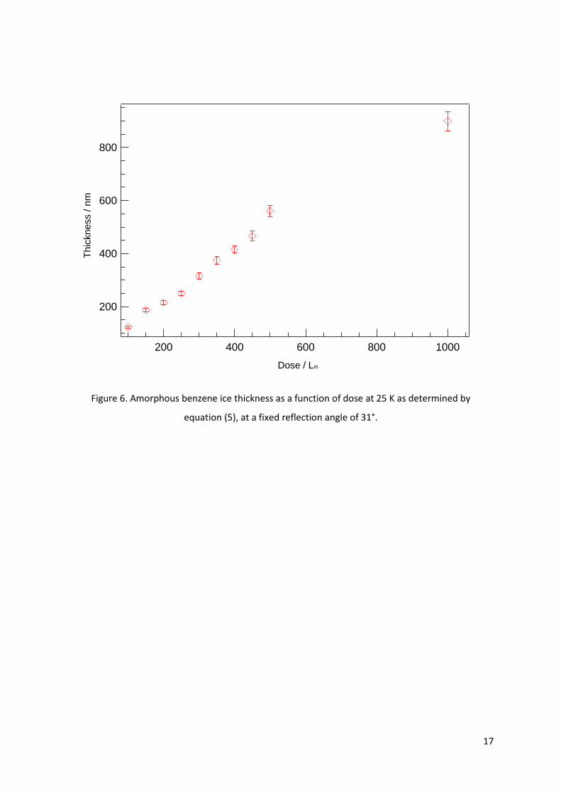
Using this mean value, thicknesses as both a function of dose at a fixed angle and as a function of

angle at a fixed dose can be determined using equation (5). Error values are calculated using the upper

and lower values of n. Figure 6 shows the determined thicknesses of doses from 100 Lm – 1000 Lm at

the narrowest reflection angle of 31°. An expected linear relationship is observed as the surface

concentration is known to be proportional to the dose.39 Similarly, at a fixed dose with varying angle,

the determined thickness should be equal within error. Indeed this is shown to be the case in Figure

7 for a dose of 250 Lm of benzene on HOPG.

Conclusions and Future Work

The data presented herein are a proof of concept of a novel UV/visible reflection-absorption

spectrometer. By employing the method outlined by Harrick,31 values for n and d for amorphous

benzene ices grown on HOPG at 25 K have been determined. The mean value for n of 1.43 ± 0.07 is in

good agreement with the literature20 and is constant within error at the doses examined. Thickness

values are of the order of several 100 nm, as expected by the appearance of interference fringes. A

linear increase of thickness with dose is observed, in line with expectations. Additionally, little

variation of thickness at a constant dose as a function of angle is found to occur.

The novel apparatus overcomes several issues identified in the introduction. In our experiment, n and

d are measured directly, eliminating the need to use an assumed value of n. Additionally, a single set

of measurements can be used to obtain both n and d, reducing experimental time. And finally,

because our interference spectra are recorded after dosing, rather than during dosing, the effect of

processing (such as annealing) on the ice in terms of n and d can be measured.

In upcoming work, the spectrometer will be used to examine other molecules and systems relevant

to astrophysical environments. These include layered and mixed ices of benzene and water. The next

stage of analysis of the data collected by the spectrometer is to determine the imaginary part, k, of

the complex refractive index, N, and hence N itself. The determined parameters can then be

incorporated into astronomical models.

Acknowledgements

JWS thanks the University of Sussex for funding. This work is funded by the STFC under grant numbers

ST/M000869/1 and ST/M001075/1 at Sussex and Heriot-Watt respectively. STFC also funded a

studentship for ST and a post-doctoral fellowship for TLS under these grant codes.

9

References

1 Y. Nakamura, Y. Katayama, and K. Hirakawa, J. Volcanol. Geotherm. Res. 114, 499 (2002).

2 K. Kourtakis, M. Lewittes, B.-L. Yu, and S. Subramoney, J. Coatings Technol. Res. 13, 953 (2016).

3 M.-J. Choi, O.D. Kwon, S.D. Choi, J.-Y. Baek, K.-J. An, and K.-B. Chung, Appl. Sci. Converg. Technol. 25,

73 (2016).

4 S.M. Mokhtar, H.M. Swailam, and H.E.-S. Embaby, Food Chem. 248, 1 (2018).

5 Z. Yue, G. Xue, J. Liu, Y. Wang, and M. Gu, Nat. Commun. 8, 15354 (2017).

6 R. Forker, M. Gruenewald, and T. Fritz, Annu. Reports Sect. “C” (Physical Chem.) 108, 34 (2012).

7 D.J. Burke and W.A. Brown, Phys. Chem. Chem. Phys. 12, 5947 (2010).

8 P. Ehrenfreund, L. d’Hendecourt, S. Charnley, and R. Ruiterkamp, J. Geophys. Res. Planets 106, 33291

(2001).

9 D.M. Hudgins, S.A. Sandford, L.J. Allamandola, and A.G.G.M. Tielens, Astrophys. J. Suppl. Ser. 86, 713

(1993).

10 W.R.M. Rocha, S. Pilling, A.L.F. de Barros, D.P.P. Andrade, H. Rothard, and P. Boduch, Mon. Not. R.

Astron. Soc. 464, 754 (2017).

11 B.S. Berland, D.R. Haynes, K.L. Foster, M.A. Tolbert, S.M. George, and O.B. Toon, J. Phys. Chem. 98, 4358

(1994).

12 W.R.M. Rocha and S. Pilling, Spectrochim. Acta. A. Mol. Biomol. Spectrosc. 123, 436 (2014).

13 G.A. Baratta and M.E. Palumbo, J. Opt. Soc. Am. A 15, 3076 (1998).

14 M.H. Moore, R.F. Ferrante, W. James Moore, and R. Hudson, Astrophys. J. Suppl. Ser. 191, 96 (2010).

15 J. Elsila, L.J. Allamandola, and S.A. Sandford, Astrophys. J. 479, 818 (1997).

16 R. Luna, M.Á. Satorre, M. Domingo, C. Millán, and C. Santonja, Icarus 221, 186 (2012).

17 M.Á. Satorre, M. Domingo, C. Millán, R. Luna, R. Vilaplana, and C. Santonja, Planet. Space Sci. 56, 1748

(2008).

18 M.S. Westley, G.A. Baratta, and R.A. Baragiola, J. Chem. Phys. 108, 3321 (1998).

19 D.M. Paardekooper, G. Fedoseev, A. Riedo, and H. Linnartz, Astron. Astrophys. 596, A72 (2016).

20 A. Dawes, N. Pascual, S. V. Hoffmann, N.C. Jones, and N.J. Mason, Phys. Chem. Chem. Phys. 19, 27544

(2017).

21 M. Elisabetta Palumbo, G.A. Baratta, M.P. Collings, and M.R.S. McCoustra, Phys. Chem. Chem. Phys. 8, 279

(2006).

22 R. Ruiterkamp, Z. Peeters, M.H. Moore, R.L. Hudson, and P. Ehrenfreund, Astron. Astrophys. 440, 391

(2005).

23 A. Rosu-Finsen, D. Marchione, T.L. Salter, J.W. Stubbing, W.A. Brown, and M.R.S. McCoustra, Phys.

Chem. Chem. Phys. 18, 31930 (2016).

24 D.J. Burke, F. Puletti, P.M. Woods, S. Viti, B. Slater, and W.A. Brown, J. Phys. Chem. A 119, 6837 (2015).

25 S. Pilling, E. Seperuelo Duarte, A. Domaracka, H. Rothard, P. Boduch, and E.F. da Silveira, Astron.

Astrophys. 523, A77 (2010).

26 S. Pilling, E. Seperuelo Duarte, E.F. da Silveira, E. Balanzat, H. Rothard, A. Domaracka, and P. Boduch,

Astron. Astrophys. 509, A87 (2010).

27 E. Dartois, J.J. Ding, A.L.F. de Barros, P. Boduch, R. Brunetto, M. Chabot, A. Domaracka, M. Godard, X.Y.

Lv, C.F. Mejía Guamán, T. Pino, H. Rothard, E.F. da Silveira, and J.C. Thomas, Astron. Astrophys. 557, A97

10

(2013).

28 A. Bergantini, S. Pilling, H. Rothard, P. Boduch, and D.P.P. Andrade, Mon. Not. R. Astron. Soc. 437, 2720

(2014).

29 C. Romanescu, J. Marschall, D. Kim, A. Khatiwada, and K.S. Kalogerakis, Icarus 205, 695 (2010).

30 K. Ishikawa, H. Yamano, K. Kagawa, K. Asada, K. Iwata, and M. Ueda, Opt. Lasers Eng. 41, 19 (2004).

31 N.J. Harrick, Appl. Opt. 10, 2344 (1971).

32 F. Carreño, J.C. Martínez‐Antón, and E. Bernabeu, Rev. Sci. Instrum. 65, 2489 (1994).

33 J. Cernicharo, A.M. Heras, A.G.G.M. Tielens, J.R. Pardo, F. Herpin, M. Guélin, and L.B.F.M. Waters,

Astrophys. J. 546, L123 (2001).

34 A.J. Remijan, F. Wyrowski, D.N. Friedel, D.S. Meier, and L.E. Snyder, Astrophys. J. 626, 233 (2005).

35 S.E. Malek, J. Cami, and J. Bernard-Salas, Astrophys. J. 744, 16 (2012).

36 J. Bernard-Salas, E. Peeters, G.C. Sloan, J. Cami, S. Guiles, and J.R. Houck, Astrophys. J. 652, L29 (2006).

37 J.D. Thrower, M.P. Collings, F.J.M. Rutten, and M.R.S. McCoustra, J. Chem. Phys. 131, 244711 (2009).

38 D. Marchione, J.D. Thrower, and M.R.S. McCoustra, Phys. Chem. Chem. Phys. 18, 4026 (2016).

39 J.D. Thrower, M.P. Collings, and F.J.M. Rutten, Mon. Not. R. Astron. Soc. 394, 1510 (2009).

40 T.L. Salter, J.W. Stubbing, L. Brigham, and W.A. Brown, In Preparation.

41 L.J. Allamandola, A.G.G.M. Tielens, and J.R. Barker, Astrophys. J. Suppl. Ser. 71, 733 (1989).

42 A.G.G.M. Tielens, Annu. Rev. Astron. Astrophys. 46, 289 (2008).

43 A.S. Bolina, A.J. Wolff, and W.A. Brown, J. Phys. Chem. B 109, 16836 (2005).

44 B.T. Draine, Annu. Rev. Astron. Astrophys. 41, 241 (2003).

45 https://oceanoptics.com/product/dh-2000-family/ Accessed May 2017

46 T. Etzkorn, B. Klotz, S. Sørensen, I. V Patroescu, I. Barnes, K.H. Becker, and U. Platt, Atmos. Environ. 33,

525 (1999).

47 E. Hecht, Optics, 4th ed. (Addison Wesley, San Francisco, 2002).

11

Tables and Figures

Table 1: Change in the angle of incidence and reflection,, with compression (+) or extension (-) of

the external linear drive on the spectrometer, according to equation (2).

x / mm / °

+15 30

+10 35

+5 40

0 45

-5 50

-10 56

-15 70

-20 75

12

Figure 1. Sketch and photographs of the apparatus. A: sketch of the design of the rhombic

construction used in the UV/visible apparatus. The symbols relate to those in equation (2). B and C:

photographs of the completed UHV assembly showing the variable rhombic system that provides the

angular variation through a linear adjustment external to the UHV system.

13

Figure 2. Measured reflection angle from the surface normal as a function of z-shift position with

corresponding Δx values. The zero position at Δx = 0 as given by equation (2) is at a z-shift reading of

120 mm.

70

60

50

40

30

145140135130125120115110105

-25-20-15-10-5051015

z-shift postion / mm

Re

fle

ctio

n a

ng

le / º

x / mm

14

Figure 3. Unprocessed UV/visible reflection spectra recorded at a reflection angle of 39°. Blue:

Background spectrum of the clean HOPG surface. Red: After direct dosing of 400 Lm of benzene. The

features at 486 nm, 581 nm and 656 nm are hydrogen emission lines from the light source output.45

200

150

100

50

0

900800700600500400300200

Bare HOPG 400 Lm Benzene

Wavelength / nm

Re

fle

ctio

n in

ten

sity / x

10

3 c

ou

nts

15

Figure 4. Reflectance spectra of 400 Lm of amorphous benzene on HOPG at two reflection angles of

31° (red trace) and 46° (black trace). The symbols refer to the terms in equations (4) and (5).

800700600500400300200

= 31º

= 46º

Wavelength / nm

R

/R

16

Figure 5. Refractive index n as a function of dose at 25 K for amorphous benzene on HOPG as

determined by equation (4).

2.2

2.0

1.8

1.6

1.4

1.2

1.0

0.8

1000800600400200

n

Dose / Lm

17

Figure 6. Amorphous benzene ice thickness as a function of dose at 25 K as determined by

equation (5), at a fixed reflection angle of 31°.

800

600

400

200

1000800600400200

Dose / Lm

Thic

kness / n

m

18

Figure 7. Amorphous benzene ice thickness as determined from equation (5) as a function of

reflection angle for a fixed dose of 250 Lm. The mean thickness is 261 ± 5 nm.

350

300

250

200

150

706560555045403530

Reflection angle / °

Th

ickn

ess /

nm