1Imaging Informatics Division, Bioinformatics Institute 30 Biopolis Street, Singapore 1386712Neural Stem Cell Laboratory, Institute of Medical Biology 8A Biomedical Grove, Singapore
Abstract: Microscopy has become a de facto tool for biology. However,it suffers from a fundamental problem of poor contrast with increasingdepth, as the illuminating light gets attenuated and scattered and hence cannot penetrate through thick samples. The resulting decay of light intensitydue to attenuation and scattering varies exponentially across the image. Theclassical space invariant deconvolution approaches alone are not suitablefor the restoration of uneven illumination in microscopy images. In thispaper, we present a novel physics-based field theoretical approach to solvethe contrast degradation problem of light microscopy images. We haveconfirmed the effectiveness of our technique through simulations as well asthrough real field experimentations.
OCIS codes: (100.2000) Digital image processing; (100.3020) Image reconstruction-restoration; (110.0180) Microscopy; (000.3860) Mathematical methods in physics.
References and links1. James B. Pawley ed. Handbook of Biological Confocal Microscopy Third Edition (Springer, New York, 2005).2. D. Kundur, D. Hatzinakos, “Blind image deconvolution”, IEEE Signal Process. Mag. pp. 43–64, May 1996).3. P. Shaw, “Deconvolution in 3-D optical microscopy,” Histochem. J. 26 1573–6865 (1994).4. P. Sarder, and A. Nehorai, “Deconvolution methods for 3-D fluorescence microscopy images,” IEEE Signal
Process. Mag. pp. 32–45, May 2006.5. J. P. Oakley and B. L. Satherley, “Improving image quality in poor visibility conditions using a physical model
for degradation,” IEEE Trans. Image Process 7(2), 167-179 (1998).6. K. Tan and J. P. Oakley, “Enhancement of color images in poor visibility conditions,” Proc. Int’l Conf. Image
Process. 2, 788-791 (2000).7. K. Tan and J. P. Oakley, “Physics Based Approach to color image enhancement in poor visibility conditions,” J.
Optical Soc. Am. 18(10), 2460–2467 (2001).8. Y. Y. Schechner, S. G. Narasimhan, and S. K. Nayar, “Polarization based vision through haze,” Appl. Opt. 42(3),
511–525 (2003).9. Y. Y. Schechner, and N. Karpel, “Clear underwater vision,” Proc. IEEE Conf. Computer Vision and Pattern
Recognition 1, 536–543 (2004).10. S. G. Narasimhan and S. K. Nayar, “Contrast restoration of weather degraded images,” IEEE Trans. Pattern Anal.
Mach. Intell 25(6), 713–724 (2003).11. S. G. Narasimhan and S. K. Nayar, “Vision and the atmosphere,” Int’l J. Computer Vision 48(3), 233–254 (2002).12. S. G. Narasimhan and S. K. Nayar, “Removing weather effects from monochrome images,” Proc. IEEE Conf.
Computer Vision and Pattern Recognition 2, 186–193 (2001).
(C) 2009 OSA 6 July 2009 / Vol. 17, No. 14 / OPTICS EXPRESS 11294#110784 - $15.00 USD Received 29 Apr 2009; revised 16 Jun 2009; accepted 18 Jun 2009; published 22 Jun 2009
13. S. G. Narasimhan and S. K. Nayar, “Chromatic framework for vision in bad weather,” Proc. IEEE Conf. ComputerVision and Pattern Recognition 1 598–605 (2000).
14. R. Kaftory, Y. Y. Schechner, and Y. Y. Zeevi, “Variational distance-dependent image restoration,” Proc. IEEEConf. Computer Vision and Pattern Recognition (2007).
15. S. Geman and D. Geman, “Stochastic relaxation, Gibbs distributions, and the Bayesian restoration of mages,”IEEE Trans. Pattern Anal. Mach. Intell 6, 721–741 (1984).
16. L. Rudin, S. Osher, and E. Fatemi, “Nonlinear total variation based noise removal algorithms,” Physica D 60259–268 (1992).
17. P. L. Combettes, and J. C. Pesquet, “Image restoration subject to a total variation constraint,” IEEE Trans. ImageProcess. 13, 1213–1222 (2004).
18. A. R. Patternson, A first course in fluid dynamics (Cambridge university press 1989).19. J. B. Pawley, Handbook of Biological Confocal Microscopy (Springer 1995).20. M. Capek, J. Janacek, and L. Kubinova, “Methods for compensation of the light attenuation with depth of images
captured by a confocal microscope,” Microscopy Res. Tech. 69, 624–635 (2006).21. P. S. Umesh Adiga and B. B. Chaudhury, “Some efficient methods to correct confocal images for easy interpre-
tation,” Micron. 32, 363–370 (2001).22. K. Greger, J. Swoger, and E. H. K. Stelzer, “Basic building units and properties of a fluorescence single plane
illumination microscope,” Rev. Sci. Instrum 78, 023705 (2007).23. J. Huisken, J. Swoger, F. Del Bene, J. Wittbrodt, and E. H. K. Stelzer, “Optical sectioning deep inside live
embryos by selective plane illumination microscopy,” Science 305, 1007–1009 (2004).24. P. J. Verveer, J. Swoger1, F. Pampaloni, K. Greger, M. Marcello, E. H. K. Stelzer. “High-resolution threedimen-
sional imaging of large specimens with light sheet-based microscopy,” Nature Methods 4(4), 311–313 (2007).25. P. J. Keller, F. Pampaloni, E. H. K. Stelzer, “Life sciences require the third dimension,” Curr. Opin. Cell Biol. 18,
117–124 (2006).26. J. G. Ritter, R. Veith, J. Siebrasse, U. Kubitscheck. “High-contrast single-particle tracking by selective focal
Microscopy [1] is an important optical imaging technique for biology. While there are manymicroscopy techniques such as two photons and single plane illumination microscopy, confocalmicroscopy has become a de facto tool for bioimaging. In confocal microscopy, out-of-focuslight are eliminated through the use of a pin-hole. Incident illuminating light passes through apin-hole and gets focused into a small region in the sample. Thus only scattered light that travelsalong the same path of the incident illuminating light passes through the pin-hole and gets fo-cused again at the light detector. The images acquired through a confocal microscope is sharperthan those produced by conventional wide-field microscopes. However, the fundamental prob-lem in confocal microscopy is the light penetration problem. Incident light gets attenuated andscattered and hence it cannot penetrate through thick samples. Generally, images acquired fromregions deep into the sample appears exponentially darker than that regions near the surface ofthe sample. Difficulties in light penetration are indeed, not restricted to confocal microscopy.Other light microscopy techniques, such as single plane illumination microscopy and wide-fieldmicroscopy suffer the same fate. The classical space invariant deconvolution approaches [2],[3], [4] are not suitable to cope with this problem of microscopy imaging.
In a seemingly totally unrelated area of research is the restoration of degraded images dueto atmospheric aerosols. This problem has been extensively studied [5], [6], [7], [8], [9], [10],[11], [12], [13] due to important applications on outdoor visions such as surveillance, navi-gation, tracking and remote sensing [5], [10]. Similar restoration techniques also found newapplications in underwater vision [8], [9], specifically for surveillance of underwater cablesand pipeline, etc. Various restoration algorithms are proposed based on physical model of lightattenuation and light scattering (airlight) through a uniform media. One of the earlier work [5]on image restoration requires accurate information of scene depths. Subsequent works cir-cumvented the need for scene depths, but require multiple images to recover the informationneeded [8], [9], [10], [14]. Narasimhan and Nayar [10], [11], [12], [13] developed an interac-tive algorithm that extracts all the required information from only one degraded image. This
(C) 2009 OSA 6 July 2009 / Vol. 17, No. 14 / OPTICS EXPRESS 11295#110784 - $15.00 USD Received 29 Apr 2009; revised 16 Jun 2009; accepted 18 Jun 2009; published 22 Jun 2009
method needs manual selection of airlight color and “good color region”. A fundamental issuewith these restoration techniques is the amplification of noise; this issue is elegantly handledby the use of a regularization term in the variational approach proposed by Kaftory et. al. [14].
Physics based restoration methods such as those described above have many advantagesover model based methods of contrast enhancement (e.g. histogram equalization). Model basedmethods [15], [16], [17] generally assume that the image properties are constant over the entireimage, this assumption is violated in weather degraded images. Moreover, physical models arebuilt upon the laws-of-physics, which we assume to be an undeniable truth.
Physics based restoration techniques had found many applications and new applications willcontinue to emerge. One amazing aspect of such restoration techniques is its validity throughseveral orders of magnitudes of physical length scales. In aerial surveillance, the physical lengthscale is of the order of ∼ 10km and in underwater surveillance, the physical length scale is ofthe order of ∼ 10m.
In this paper, we link two unrelated areas of research: restoration of images from light mi-croscopy and restoration of weather degraded images. We propose a new application for physicsbased restoration for light microscopy, which has a physical length scale of ∼ 100μm. Therebyextending the length scales of physics based restoration to 8 orders of magnitudes. We furtherimproved the physics based model with a field theoretical formulation.
Our proposed formulation is radically different from all existing physics based restora-tion techniques, in which we do not assume constant extinction coefficient in the attenuatingmedium. Moreover, in our formalism, we make no distinction between the image object andthe attenuating medium. We derived a general set of equations to handle any geometrical setupin the image acquisition. To use our method, one only need to specify details of the light sourceand the detection equipment such as a camera. We propose a different formulation because theexisting physics-based methods [5], [6], [7], [8], [9], [10], [11], [12], [13] cannot be applied tothree dimensional microscopy images. Firstly, existing methods “removes” the attenuation me-dia to retrieve a two dimensional scence. On the contrary, in this paper, the attenuation mediaalso contains the image information. We want to restore the true signals of the media insteadof removing them. Secondly, existing methods assume a uniform attenuation medium, an as-sumption that is strongly violated in microscopy images.
2. Field theoretical formulation
Our approach is formulated on strong theoretical grounds, it is based on fundemental laws-of-physics, such as conservation laws represented by the continuity equation. We use a fieldtheoretical approach that is well proven over centuries in physics.
Assume a region of interest Ω ⊂ R3 that contains the whole imaging system, including the
image object, the attenuation medium, light sources and detectors (e.g. camera). The lightsources originate from infinity, we consider them to originate from the boundary of the re-gion of interest ∂Ω. However, this is not a requirement in our formalism. Let rs ∈ Ωs be the setof points in the light sources and rp be the locations of the voxels in the detector.
2.1. Photon density and light intensity
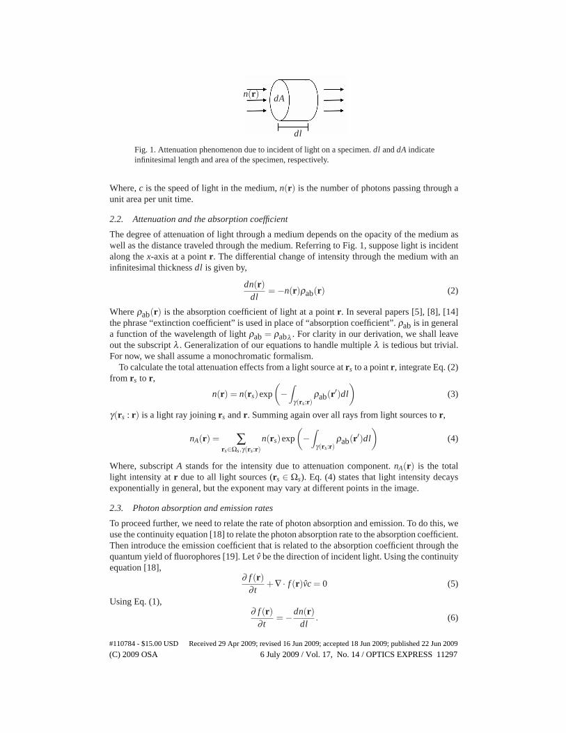
We first consider the mathematical model of photon (light) density and light intensity field. Letf (r) be the number of photons per unit volume and n(r) be the light intensity at a point r ∈ Ω.Total number of photons in an infinitesimal volume dV = dldA (Fig. 1) is f (r)dldA. In the timeinterval dt, the number of photons passing through the area dA is,
n(r)dA = f (r)dldt
dA = f (r)cdA ⇒ n(r) = f (r)c (1)
(C) 2009 OSA 6 July 2009 / Vol. 17, No. 14 / OPTICS EXPRESS 11296#110784 - $15.00 USD Received 29 Apr 2009; revised 16 Jun 2009; accepted 18 Jun 2009; published 22 Jun 2009
dAn(r)
dl
Fig. 1. Attenuation phenomenon due to incident of light on a specimen. dl and dA indicateinfinitesimal length and area of the specimen, respectively.
Where, c is the speed of light in the medium, n(r) is the number of photons passing through aunit area per unit time.
2.2. Attenuation and the absorption coefficient
The degree of attenuation of light through a medium depends on the opacity of the medium aswell as the distance traveled through the medium. Referring to Fig. 1, suppose light is incidentalong the x-axis at a point r. The differential change of intensity through the medium with aninfinitesimal thickness dl is given by,
dn(r)dl
= −n(r)ρab(r) (2)
Where ρab(r) is the absorption coefficient of light at a point r. In several papers [5], [8], [14]the phrase “extinction coefficient” is used in place of “absorption coefficient”. ρab is in generala function of the wavelength of light ρab = ρabλ . For clarity in our derivation, we shall leaveout the subscript λ . Generalization of our equations to handle multiple λ is tedious but trivial.For now, we shall assume a monochromatic formalism.
To calculate the total attenuation effects from a light source at rs to a point r, integrate Eq. (2)from rs to r,
n(r) = n(rs)exp
(−∫
γ(rs:r)ρab(r′)dl
)(3)
γ(rs : r) is a light ray joining rs and r. Summing again over all rays from light sources to r,
nA(r) = ∑rs∈Ωs,γ(rs:r)
n(rs)exp
(−∫
γ(rs:r)ρab(r′)dl
)(4)
Where, subscript A stands for the intensity due to attenuation component. nA(r) is the totallight intensity at r due to all light sources (rs ∈ Ωs). Eq. (4) states that light intensity decaysexponentially in general, but the exponent may vary at different points in the image.
2.3. Photon absorption and emission rates
To proceed further, we need to relate the rate of photon absorption and emission. To do this, weuse the continuity equation [18] to relate the photon absorption rate to the absorption coefficient.Then introduce the emission coefficient that is related to the absorption coefficient through thequantum yield of fluorophores [19]. Let v̂ be the direction of incident light. Using the continuityequation [18],
∂ f (r)∂ t
+∇ · f (r)v̂c = 0 (5)
Using Eq. (1),∂ f (r)
∂ t= −dn(r)
dl. (6)
(C) 2009 OSA 6 July 2009 / Vol. 17, No. 14 / OPTICS EXPRESS 11297#110784 - $15.00 USD Received 29 Apr 2009; revised 16 Jun 2009; accepted 18 Jun 2009; published 22 Jun 2009
dr′
n(r′)ρem(r′)dr′
rdA
‖r−r′ ‖
2
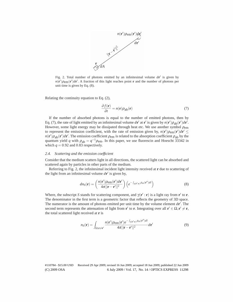
Fig. 2. Total number of photons emitted by an infinitesimal volume dr′ is given byn(r′)ρem(r′)dr′. A fraction of this light reaches point r and the number of photons perunit time is given by Eq. (8).
Relating the continuity equation to Eq. (2),
∂ f (r)∂ t
= n(r)ρab(r) (7)
If the number of absorbed photons is equal to the number of emitted photons, then byEq. (7), the rate of light emitted by an infinitesimal volume dr′ at r′ is given by n(r′)ρab(r′)dr′.However, some light energy may be dissipated through heat etc. We use another symbol ρemto represent the emission coefficient, with the rate of emission given by, n(r′)ρem(r′)dr′ ≤n(r′)ρab(r′)dr′. The emission coefficient ρem is related to the absorption coefficient ρab by thequantum yield q with ρab = q−1ρem. In this paper, we use fluorescin and Hoescht 33342 inwhich q = 0.92 and 0.83 respectively.
2.4. Scattering and the emission coefficient
Consider that the medium scatters light in all directions, the scattered light can be absorbed andscattered again by particles in other parts of the medium.
Referring to Fig. 2, the infinitesimal incident light intensity received at r due to scattering ofthe light from an infinitesimal volume dr′ is given by,
dnS(r) =(
n(r′)ρem(r′)dr′
4π||r− r′||2)(
e−∫
γ(r′:r) ρab(r′′)dl)
(8)
Where, the subscript S stands for scattering component, and γ(r′ : r) is a light ray from r′ to r.The denominator in the first term is a geometric factor that reflects the geometry of 3D space.The numerator is the amount of photons emitted per unit time by the volume element dr′. Thesecond term represents the attenuation of light from r′ to r. Integrating over all r′ ∈ Ω,r′ = r,the total scattered light received at r is
nS(r) =∫
Ω,r=r′n(r′)ρem(r′)e−
∫γ(r′:r) ρab(r′′)dl
4π||r− r′||2 dr′ (9)
(C) 2009 OSA 6 July 2009 / Vol. 17, No. 14 / OPTICS EXPRESS 11298#110784 - $15.00 USD Received 29 Apr 2009; revised 16 Jun 2009; accepted 18 Jun 2009; published 22 Jun 2009
2.5. Image formation
We can write the total light intensity at a point r ∈ Ω as a sum of attenuation and scatteringcomponents.
n(r) = nA(r)+nS(r)
= ∑rs∈Ωs,γ(rs:r)
n(rs)e−∫γ(rs:r) ρab(r′)dl
+∫
r=r′n(r′)ρem(r′)e−
∫γ(r′:r) ρab(r′′)dl
4π||r− r′||2 dr′
(10)
Finally, we relate our physical model to the observed image. The total amount of light emittedper unit time by an infinitesimal volume dr is ρem(r)n(r)dr. Suppose the detector detects a partof this light to form pixel rp in the 3-dimensional observed image u0 (for example, in confocalmicroscopy), the pixel intensity at rp is given by,
u0(rp) =∫
r∈Ω,γ(r:rp)αγ ρem(r)n(r)e−
∫γ ρab(r′)dldr (11)
the integral is over all light rays from all points r ∈ Ω to rp. The attenuation term appears againin this equation as light is attenuated when traveling from the medium location r to the pixellocation rp. αγ = αγ(r,rp) is a function that depends on the lensing system of the detector. Thesubscript γ is used to indicate that αγ depends on the path of the light.
Objective of imaging is to find out what objects are present in the region of interest Ω, inother words, we want to measure the optical properties of materials in Ω. These properties aregiven by ρab(r) and ρem(r). Thus we want to estimate ρab(r) and ρem(r) given the observedimage u0(rp). To this end, we want to solve Eq (11) for ρab(r) and ρem(r). At first sight, thisequation seems non-invertible and its solution may not be unique. In the latter sections, we willillustrate examples in which we solve Eq. (11) for confocal microscopy and for a side scatteringconfiguration. At this point, we would like to highlight several observations:
1. Geometry: All geometrical information is embedded in the paths γ(r : r′), which repre-sents light rays from point r to r′.
2. Light Source: Light source information is given by the summation over Ωs and γ(rs : r)in Eq. (4).
3. Airlight: The airlight effect [10] is included in our scattering term (Eq. (10)).
4. Non-unique solution: The solution of Eq. (11) is non-unique in general. Consider a casewhen Ω contains an opaque box and an image is taken of this box. Since the box isopaque, the values of ρab and ρem within the box are undefined.
2.6. Discretization
We derived a matrix equation by discretizing the total light intensity (Eq. (10)) at each pointr. We perform our discretization such that each finite-element corresponds to one voxel inthe image data. Let bi = nA(ri), b = (b1, · · · ,bN), N is the total number of voxels. Next defineui/ρem(ri) = n(ri), u = (u1, · · · ,uN). Finally, define a matrix G with components Gi j = (ri,r j),
G(ri,r j) =
⎧⎪⎪⎨⎪⎪⎩
− exp(−∑rk∈γ(r j :ri)
ρab(rk)Δrk
)4π||ri−r j ||2 ΔV i = j
1ρem(ri)
i = j
(12)
(C) 2009 OSA 6 July 2009 / Vol. 17, No. 14 / OPTICS EXPRESS 11299#110784 - $15.00 USD Received 29 Apr 2009; revised 16 Jun 2009; accepted 18 Jun 2009; published 22 Jun 2009
Then Eq. (10) reduces to,
ui
ρem(ri)= bi + ∑
j =i
⎛⎝+
exp(
∑rk∈γ(r j :ri) ρab(rk)Δrk
)4π||ri − r j||2 ΔV
⎞⎠u j
⇒ G ·u = b (13)
It will be demonstrated in later sections that this matrix equation is convenient for subsequentcalculations.
3. Confocal microscopy
Confocal microscopy [1] is one of the most important tool in bioimaging. Images acquiredthrough a confocal microscope is much sharper than images from conventional wide-field mi-croscope. However, degradation by light attenuation effect is acute in confocal microscopy.This problem has been inadequately handled by either increasing the laser power or increasingthe sensitivity of the photomultiplier tube [20]. Both techniques are inadequate and have draw-backs: increasing laser power accelerates photo-bleaching effects and increasing the sensitivityof the photo-multiplier tube adds noise. In the past, Umesh Adiga and B. B. Chaudhury [21]discussed the use of simple thresholding method to separate background from foreground forrestoring images from light attenuation along the depth of the image stack. This technique mak-ing an assumption that image voxels are isotropic (which is not true for confocal microscopy)based on XOR contouring and morphing to virtually insert the image slices in the image stackfor improving axial resolution.
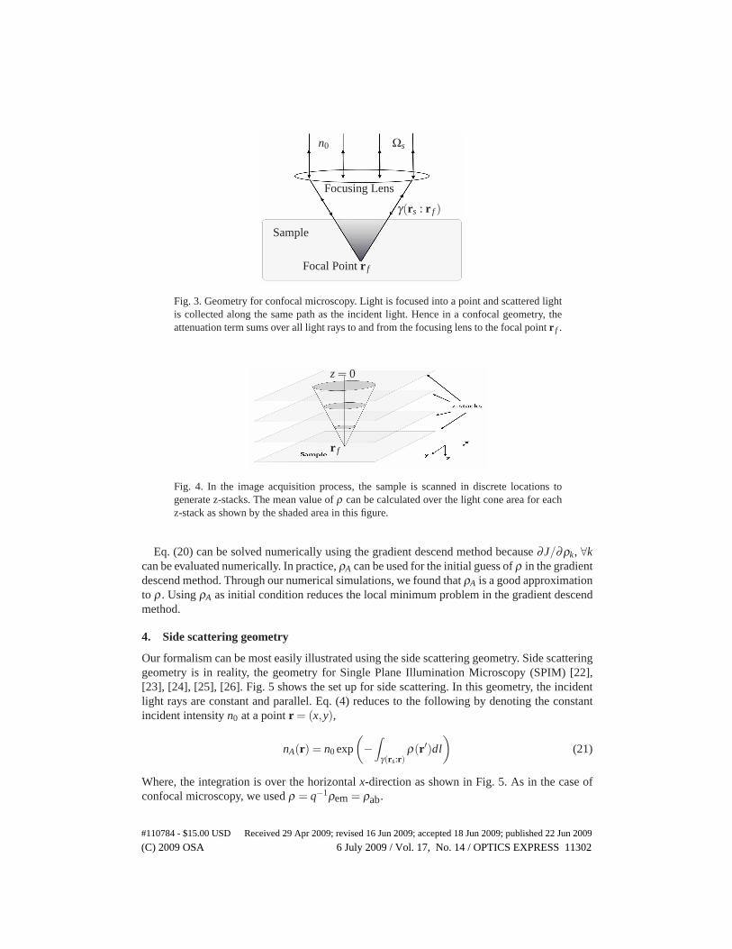
Fig. 3 shows the geometry for confocal microscopy setup. Incident light passes through thefocusing lens and is focused at the point r f . The summation over all light rays in Eq. (4) sumsover all rays from the focusing lens γ(rs : r f ). We can take the area of the lens to be a set ofpoints in the incident light sources Ωs. Detected light travels via the same paths through thefocusing lens. Hence the summation over all light rays in Eq. (11) sums over the same pathsγ(r f : rs) but in the opposite direction. Lastly, for clarity, define the symbol ρ(r) = ρab(r) =q−1ρem(r).
We can use an approximation to simplify Eq. (4) and (11) by calculating the mean ρ(r) overthe disk area of light cones for each z-stacks (shaded gray in Fig. 4).
〈ρ〉(z) =∫
diskdxdyρ(x,y,z)∫
diskdxdy
(14)
Then Eq. (4) becomes
nA(r) = n0 ∑rs∈Ωs;γ(rs:r)
exp
(−∫
γ(rs:r)ρ(r′)dl
)
≈ n0 exp
(−∫ r f
z=0〈ρ〉(z)dz
)∑
rs∈Ωs;γ(rs:r)
= βn0 exp
(−∫ r f
z=0〈ρ〉(z)dz
)(15)
Here we assume a constant incident light intensity at the focusing lens (n0). β = ∑rs∈Ωs,γ(rs:r) isa complicated function of the light paths but is a constant number as long as the focal length ofthe focusing lens does not change. For confocal microscopy, only light emitted at r f is collected
(C) 2009 OSA 6 July 2009 / Vol. 17, No. 14 / OPTICS EXPRESS 11300#110784 - $15.00 USD Received 29 Apr 2009; revised 16 Jun 2009; accepted 18 Jun 2009; published 22 Jun 2009
by the photomultiplier (see Fig. 3). Hence replacing the ρ in Eq. (11) by 〈ρ〉 defined in Eq. (14),we have,
u0(rp) =∫
r∈Ω,γ(r:rp)αγq−1ρ(r)n(r)e−
∫γ ρ(r′)dldr
≈ n(r f )ρ(r f )e−∫ r fz=0〈ρ〉dz ∑
γ(r f ,rp)q−1αγ ΔVf
= α ′u(r f )e−∫ r fz=0〈ρ〉(z)dz (16)
ΔVf is the confocal volume and α ′ = ∑γ(r f ,rp) q−1αγ ΔVf is complicated but otherwise constantnumber. We have also use u(r) = ρ(r)n(r).
An analytic solution can be obtained if we neglect the scattering terms (nS � nA, n(r) ∼=nA(r)). Substituting Eqs. (15) and (16) into Eq. (13),
ρA(ri) =u0i
α ′βn0exp
(2∫ zi
z=0〈ρ〉(z)dz
)(17)
ρA is the true light emission coefficient we are solving for if we neglect the scattering terms.We now give a description of how ρA can be calculated from the observed image slice-by-slicethrough the z-stack. ρA is calculated starting from the first slice.
1. For the first slice, z = 0, the integral in Eq. (17) evaluates to zero so that ρA is proportionalto the intensity in the observed image.a i.e. ρA(ri,z = 0) = u0i/α ′βn0.
2. ρA for the second slice depends on ρA for the first slice,
ρA(ri,z = 1) =u0i
α ′βn0exp[2〈ρA〉(z = 0)Δz] (18)
Δz is the thickness of the discretized z-stack. 〈ρA〉(z = 0) is an average value calculatedusing values of ρA for the first slice.
3. ρA for the k-th slice is given by,
ρA(ri,z = k) =u0i
α ′βn0exp
(2
k−1
∑z=0
〈ρA〉(z)Δz
)(19)
since we calculate the values of ρA slice-by-slice starting from the first slice, thevalues of ρA had been calculated for all (k− 1)th slice and hence the exponential term,∑k−1
z=0 2〈ρA〉(z)Δz can be calculated easily.
Thus we calculate ρA from first to last slice in sequence to obtain the whole restored image.Inclusion of the scattering term results in non-analytic solutions, which can be solved numer-
ically by,
J(ρ) = ‖b−G ·u‖ρ∗ = |argmin
ρJ(|ρ|)| (20)
since ρ > 0, we use the absolute sign to avoid the Karush-Kuhn-Tucker condition. In the aboveequation bi = b(ri) = nA(ri) (Eq. (15)) and ui = u(ri) = u0(ri)exp(
∫ r fz=0〈ρ〉dz)/α ′ (Eq. (16)).
To reduce computation time, we do sampling in calculating the mean ρ(r) over the disk area oflight cones for each z-stacks.
(C) 2009 OSA 6 July 2009 / Vol. 17, No. 14 / OPTICS EXPRESS 11301#110784 - $15.00 USD Received 29 Apr 2009; revised 16 Jun 2009; accepted 18 Jun 2009; published 22 Jun 2009
n0
Sample
Focusing Lens
Focal Point r f
Ωs
γ(rs : r f )
Fig. 3. Geometry for confocal microscopy. Light is focused into a point and scattered lightis collected along the same path as the incident light. Hence in a confocal geometry, theattenuation term sums over all light rays to and from the focusing lens to the focal point r f .
z = 0
r f
Fig. 4. In the image acquisition process, the sample is scanned in discrete locations togenerate z-stacks. The mean value of ρ can be calculated over the light cone area for eachz-stack as shown by the shaded area in this figure.
Eq. (20) can be solved numerically using the gradient descend method because ∂J/∂ρk, ∀kcan be evaluated numerically. In practice, ρA can be used for the initial guess of ρ in the gradientdescend method. Through our numerical simulations, we found that ρA is a good approximationto ρ . Using ρA as initial condition reduces the local minimum problem in the gradient descendmethod.
4. Side scattering geometry
Our formalism can be most easily illustrated using the side scattering geometry. Side scatteringgeometry is in reality, the geometry for Single Plane Illumination Microscopy (SPIM) [22],[23], [24], [25], [26]. Fig. 5 shows the set up for side scattering. In this geometry, the incidentlight rays are constant and parallel. Eq. (4) reduces to the following by denoting the constantincident intensity n0 at a point r = (x,y),
nA(r) = n0 exp
(−∫
γ(rs:r)ρ(r′)dl
)(21)
Where, the integration is over the horizontal x-direction as shown in Fig. 5. As in the case ofconfocal microscopy, we used ρ = q−1ρem = ρab.
(C) 2009 OSA 6 July 2009 / Vol. 17, No. 14 / OPTICS EXPRESS 11302#110784 - $15.00 USD Received 29 Apr 2009; revised 16 Jun 2009; accepted 18 Jun 2009; published 22 Jun 2009
Fig. 5. Geometrical arrangement of side scattering, the light source originates from theside and illuminates one plane of the sample. Scattered light is collected in an orthogonaldirection by a CCD camera.
Assume the scattered light travels directly to the CCD camera without attenuation. As inmost camera set up, let there be a one-to-one correspondence between the pixel point (in theCCD) rp and the sample location r. Then Eq. (11) may be written as,
u0(r) = α ′ρ(r)n(r) = α ′u(r) (22)
Where, α ′ represents the integrated effects of quantum yield and the camera, including sum-mations over all rays etc. An analytic solution can be obtained (Eq. (23)) if we further ignorethe scattering term,
ρA(ri) =1
α ′n0u0(ri)exp
(∑
rk∈γ(rs,ri)ρ(rk)Δrk
)(23)
Where, the subscript A is used to indicate that an approximated solution is obtained usingattenuation term only. With this approximation, Eq. (23) can be easily solved numerically andtheir results are given in the next section.
In our numerical experiments, we observed that the restored image using Eq. (23) andEq. (20) differs by about 1% only, which suggest that our approximation nS � nA is valid.
5. Results
We performed numerical calculations and compare our results to ground truths. Comparisonwith other physics-based restoration methods [5], [6], [7], [8], [9], [10], [11], [12], [13] is notpossible because these methods cannot be applied to microscopy images. Firstly, other physics-based methods are not designed to restore three dimensional images. Secondly, these methodsassumes a constant attenuation media. An assumption that is strongly violated in microscopyimages.
5.1. Validation and calibration
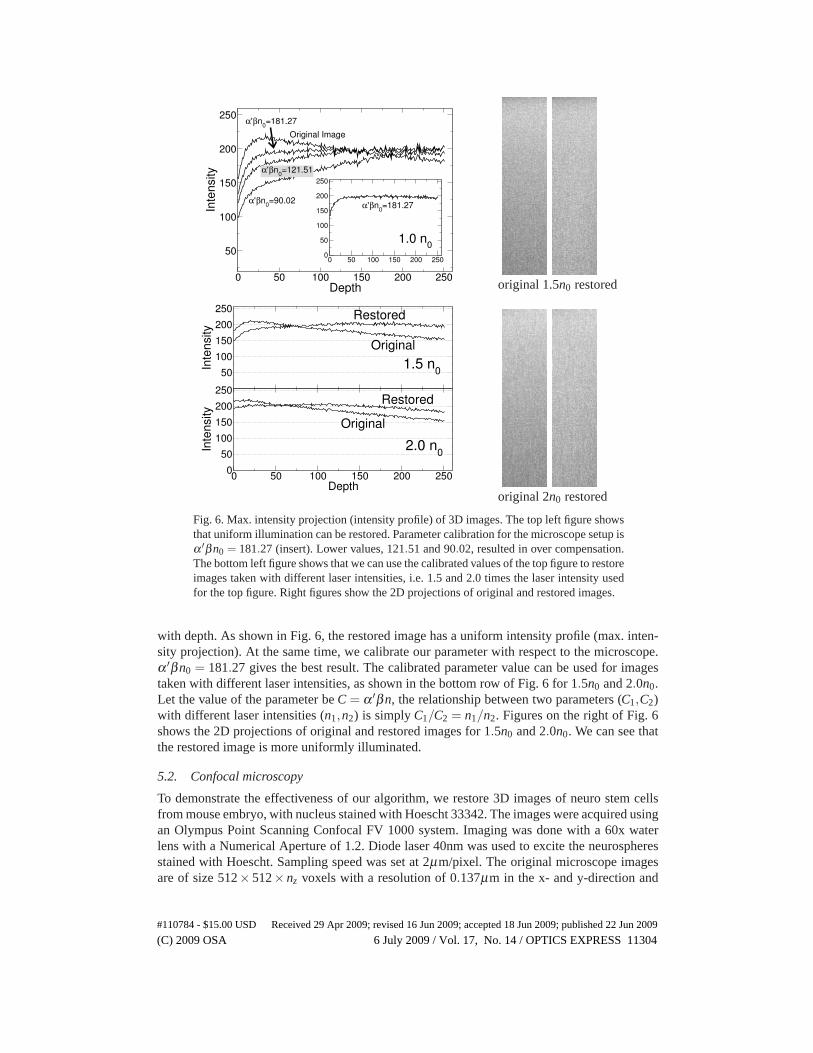
We validate our method on specially prepared samples in which we know the ground truth byexperimental design. Image restoration is then performed and compared to the ground truth.In the experiment, we mix fluorescein and liquid gel on an orbital shaker until the gel hard-ens. In this way, we are absolutely sure that the sample is uniform through-out the 3D volume.However, the intensity profile of the image will not be uniform due to attenuation, it decreases
(C) 2009 OSA 6 July 2009 / Vol. 17, No. 14 / OPTICS EXPRESS 11303#110784 - $15.00 USD Received 29 Apr 2009; revised 16 Jun 2009; accepted 18 Jun 2009; published 22 Jun 2009
original 1.5n0 restored
original 2n0 restored
Fig. 6. Max. intensity projection (intensity profile) of 3D images. The top left figure showsthat uniform illumination can be restored. Parameter calibration for the microscope setup isα ′βn0 = 181.27 (insert). Lower values, 121.51 and 90.02, resulted in over compensation.The bottom left figure shows that we can use the calibrated values of the top figure to restoreimages taken with different laser intensities, i.e. 1.5 and 2.0 times the laser intensity usedfor the top figure. Right figures show the 2D projections of original and restored images.
with depth. As shown in Fig. 6, the restored image has a uniform intensity profile (max. inten-sity projection). At the same time, we calibrate our parameter with respect to the microscope.α ′βn0 = 181.27 gives the best result. The calibrated parameter value can be used for imagestaken with different laser intensities, as shown in the bottom row of Fig. 6 for 1.5n0 and 2.0n0.Let the value of the parameter be C = α ′βn, the relationship between two parameters (C1,C2)with different laser intensities (n1,n2) is simply C1/C2 = n1/n2. Figures on the right of Fig. 6shows the 2D projections of original and restored images for 1.5n0 and 2.0n0. We can see thatthe restored image is more uniformly illuminated.
5.2. Confocal microscopy
To demonstrate the effectiveness of our algorithm, we restore 3D images of neuro stem cellsfrom mouse embryo, with nucleus stained with Hoescht 33342. The images were acquired usingan Olympus Point Scanning Confocal FV 1000 system. Imaging was done with a 60x waterlens with a Numerical Aperture of 1.2. Diode laser 40nm was used to excite the neurospheresstained with Hoescht. Sampling speed was set at 2μm/pixel. The original microscope imagesare of size 512× 512× nz voxels with a resolution of 0.137μm in the x- and y-direction and
(C) 2009 OSA 6 July 2009 / Vol. 17, No. 14 / OPTICS EXPRESS 11304#110784 - $15.00 USD Received 29 Apr 2009; revised 16 Jun 2009; accepted 18 Jun 2009; published 22 Jun 2009
(a) Original view
(b) Restored view, 1/α ′βn0 = 0.014995
(c) Maximum intensity projection
Las
erD
irec
tion
�
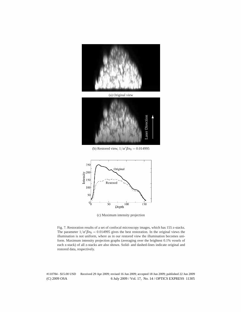
Fig. 7. Restoration results of a set of confocal microscopy images, which has 155 z-stacks.The parameter 1/α ′βn0 = 0.014995 gives the best restoration. In the original views theillumination is not uniform, where as in our restored view the illumination becomes uni-form. Maximum intensity projection graphs (averaging over the brightest 0.1% voxels ofeach z-stack) of all z-stacks are also shown. Solid- and dashed-lines indicate original andrestored data, respectively.
(C) 2009 OSA 6 July 2009 / Vol. 17, No. 14 / OPTICS EXPRESS 11305#110784 - $15.00 USD Received 29 Apr 2009; revised 16 Jun 2009; accepted 18 Jun 2009; published 22 Jun 2009
(a) Original view
(b) Restored view, 1/α ′βn0 = 0.014995
(c) Maximum intensity projection
Las
erD
irec
tion
�
Fig. 8. Restoration results of another set of confocal microscopy images, which consists of163 z-stacks. The parameter 1/α ′βn0 = 0.014995 gives the best restoration. In the originalviews the illumination is not uniform, where as in our restored view the illumination be-comes uniform. Maximum intensity projection graphs (averaging over the brightest 0.1%voxels of each z-stack) of all z-stacks are also shown. Solid- and dashed-lines indicateoriginal and restored data, respectively.
(C) 2009 OSA 6 July 2009 / Vol. 17, No. 14 / OPTICS EXPRESS 11306#110784 - $15.00 USD Received 29 Apr 2009; revised 16 Jun 2009; accepted 18 Jun 2009; published 22 Jun 2009
Fig. 9. Restoration of a synthetically degraded image to an image of uniform illumina-tion. The degraded image shows non-uniform illumination with maximum intensity projec-tion falling off exponentially (assuming light source comes from the left). The parameter1/α ′n0 = 0.0095 gives the best restoration in which the maximum intensity projection isflat.
0.2μm in the z-direction. nz is the number of z-stacks in the images.To reduce the computation time, in our experimentation we downsampled the original images
to 256× 256× nz voxels by averaging the voxels in the x- and y- direction while maintainingthe resolution in the z-direction. Fig. 7 and 8 show restoration results for a 256× 256× nz
voxels images. Here we used Eq. (17) to restore the images. The adjusted tuning parameter1/α ′βn0 = 0.014995 gives optimal restoration results.
The confocal images shown in Fig. 7 and 8 have nz = 155 and nz = 163 z-stacks, respectively.Fig. 7(a) and 8(a) show the maximum intensity projection onto the yz-plane of the respectiveoriginal images. Similarly, Fig. 7(b) and 8(b) show the maximum intensity projection onto theyz-plane of the respective restored images. And Fig. 7(c) and 8(c) show the maximum intensityprojection (averaged over top 0.1% of the brightest voxels in the xy-plane) onto the z-axis. Theilluminating laser originates from the bottom and one could easily observed that for the originalimage, the voxels are much brighter at the bottom of the image and intensity drops towards thetop of the image. After restoration, the illumination becomes uniform. The restored image isalso darker on the average, however, many image processing techniques are robust against theaverage voxel intensity. The achievement in our work is to restore the image to have uniformillumination. Afterwhich, other image enhancement methods such as histogram equalizationcan be used. Fig. 7(c) and 8(c) clearly show the difference between the intensity profile ofthe original (solid lines) and restored (dashed lines) images. Over-exposed areas in the bottomz-stacks are correctly compensated by our restoration method.
5.3. Side scattering microscopy
We performed calculations of side scattering geometry on synthetically degraded images. Thesynthetic image with non-uniform illumination (maximum intensity projection falling off ex-ponentially assuming light source comes from the left) was generated from an image of uni-form illumination. Fig. 9 shows restoration results for a 256×256 pixels image. Here we usedEq. (23) to restore the image. The tuning parameter 1/α ′n0 can be adjusted to obtain optimal re-sults. n0 is the incident light intensity and α ′ is a geometric factor that is usually unknown. For
(C) 2009 OSA 6 July 2009 / Vol. 17, No. 14 / OPTICS EXPRESS 11307#110784 - $15.00 USD Received 29 Apr 2009; revised 16 Jun 2009; accepted 18 Jun 2009; published 22 Jun 2009
small 1/α ′n0, the image is hardly restored and for large 1/α ′n0, there is over-compensationof the attenuation effect. The optimal value of 1/α ′n0 is 0.0095 for this image in which therestored image is almost perfectly (uniformly) illuminated.
6. Conclusions
In this paper, we addressed the fundamental light attenuation and scattering problem for lightmicroscopy, which caused non-uniformly illuminated images, by proposing a physics-basedfield theoretical restoration model. Our method has strong theoretical grounds as it is basedon well proven fundemental laws-of-physics. We presented the complete mathematical formu-lations for restoration of light microscopy images. We validated our method with a speciallydesigned experiment, and confirmed through specific examples of confocal and side scatteringgeometry, that our restoration method is efficient in solving the problem of light attenuationand scattering.
Lastly, we would like to note that existing physics-based approaches [5], [6], [7], [8], [9],[10], [11], [12], [13] cannot be use as comparisons as they are not formulated to restore thewhole three dimensional image volume, as required in microscopy images.
(C) 2009 OSA 6 July 2009 / Vol. 17, No. 14 / OPTICS EXPRESS 11308#110784 - $15.00 USD Received 29 Apr 2009; revised 16 Jun 2009; accepted 18 Jun 2009; published 22 Jun 2009