HAL Id: hal-02869326 https://hal.archives-ouvertes.fr/hal-02869326 Submitted on 15 Jul 2020 HAL is a multi-disciplinary open access archive for the deposit and dissemination of sci- entific research documents, whether they are pub- lished or not. The documents may come from teaching and research institutions in France or abroad, or from public or private research centers. L’archive ouverte pluridisciplinaire HAL, est destinée au dépôt et à la diffusion de documents scientifiques de niveau recherche, publiés ou non, émanant des établissements d’enseignement et de recherche français ou étrangers, des laboratoires publics ou privés. A first glimpse at the influence of body mass in the morphological integration of the limb long bones: an investigation in modern rhinoceroses Christophe Mallet, Guillaume Billet, Alexandra Houssaye, Raphael Cornette To cite this version: Christophe Mallet, Guillaume Billet, Alexandra Houssaye, Raphael Cornette. A first glimpse at the influence of body mass in the morphological integration of the limb long bones: an investigation in modern rhinoceroses. Journal of Anatomy, Wiley, 2020, 10.1111/joa.13232. hal-02869326
Transcript
HAL Id: hal-02869326https://hal.archives-ouvertes.fr/hal-02869326
Submitted on 15 Jul 2020
HAL is a multi-disciplinary open accessarchive for the deposit and dissemination of sci-entific research documents, whether they are pub-lished or not. The documents may come fromteaching and research institutions in France orabroad, or from public or private research centers.
L’archive ouverte pluridisciplinaire HAL, estdestinée au dépôt et à la diffusion de documentsscientifiques de niveau recherche, publiés ou non,émanant des établissements d’enseignement et derecherche français ou étrangers, des laboratoirespublics ou privés.
A first glimpse at the influence of body mass in themorphological integration of the limb long bones: an
investigation in modern rhinocerosesChristophe Mallet, Guillaume Billet, Alexandra Houssaye, Raphael Cornette
To cite this version:Christophe Mallet, Guillaume Billet, Alexandra Houssaye, Raphael Cornette. A first glimpse at theinfluence of body mass in the morphological integration of the limb long bones: an investigation inmodern rhinoceroses. Journal of Anatomy, Wiley, 2020, �10.1111/joa.13232�. �hal-02869326�
tibia, femur-fibula and tibia-fibula), serially homologous bones (humerus-femur, radius-tibia, radius-175
fibula, ulna-tibia and ulna-fibula) and functionally analogous bones (humerus-tibia, humerus-fibula) 176
(Figure 1). If the serial homology for the stylopodial bones seems obvious, no clear consensus exists 177
for the serial homology within the zeugopodium elements. Many studies consider the radius and the 178
tibia, and the ulna and the fibula, as serially homologous respectively (Bininda-Emonds et al. 2007; 179
Schmidt & Fischer 2009; Martín-Serra et al. 2015; Hanot et al. 2017; Botton-Divet et al. 2018), 180
unfortunately without strong developmental or genetic evidences. Recent studies tend to indicate 181
that the apparently obvious homology between fore- and hind limb segments might be much more 182
spurious than previously thought (Diogo & Molnar 2014; Sears et al. 2015). In this context, we 183
therefore tested the four possible bone combinations in the zeugopodium. As the appendicular 184
skeleton is known to be highly integrated among quadrupedal mammals (Schmidt & Fischer 2009; 185
Martín-Serra et al. 2015; Hanot et al. 2017; Botton-Divet et al. 2018), we also tested the 186
combinations involving non-homologous or analogous bones (radius-femur and ulna-femur) (Figure 187
1). Covariation patterns were investigated using Two-Blocks Partial Least Squares (2BPLS) analyses. 188
The 2BPLS method extracts the principal axes of covariation from a covariance matrix computed on 189
8
two shape datasets (Rohlf & Corti 2000; Botton-Divet et al. 2018; Hanot et al. 2018), allowing to 190
visualise the specimen repartition relatively to these axes and the shape changes associated. 191
Each PLS axis is characterized notably by its explained percentage of the overall covariation, its PLS 192
correlation coefficient (rPLS) and its p-value, computed as a singular warp analysis as detailed in 193
Bookstein et al. (2003). The p-value was considered as significant when the observed rPLS was higher 194
than the ones obtained from randomly permuted blocks (1000 permutations). When the p-value was 195
below 0.05, the PLS was considered as significant, i.e. the two considered blocks as significantly 196
integrated. We used the function “pls2b” in the “Morpho” package to compute the 2BPLS (Schlager 197
2017). To visualise these shape changes along the PLS axes, we used the function “plsCoVar” in the 198
“Morpho” package to compute theoretical shapes at two standard deviations on each side of each 199
axis (see Schlager, 2017). These theoretical conformations were then used to calculate a TPS 200
deformation of the template mesh and therefore visualise the shape changes along the PLS axes. We 201
then used the function “meshDist” in the “Morpho” package to create colour maps indicating the 202
location and the intensity of the covariation between two meshes by mapping the distance between 203
the minimum and maximum theoretical shapes along he first PLS axis (i.e. areas in red are the ones 204
showing the most of shape changes within a bone pair whereas the areas in blue are the ones 205
showing the less of shape change). 206
This procedure was performed at an interspecific level including all the 50 specimens into a single 207
GPA. We also explored the intraspecific level of covariation by performing the sliding and GPA 208
procedures on subsamples containing each different species. We then obtained five specific datasets 209
on which were performed 2BPLS analyses. 210
Effect of the allometry 211
It has been previously demonstrated that centroid size may be a good approximation of the body 212
mass of the specimen (Ercoli & Prevosti 2011; Cassini et al. 2012), notably among modern rhinos 213
(Mallet et al. 2019). To assess the effect of body mass on integration patterns – i.e. the effect of 214
evolutionary allometry – we computed a multivariate regression of the shape against the centroid 215
size using the function “procD.lm” in the “geomorph” package (v3.1.2—Adams & Otárola-Castillo, 216
2013). Then the residuals were used to compute allometry-free shapes, which were analysed with 217
2BPLS as described previously. Each species may have its own allometric slope, making it difficult to 218
remove the general allometry effect (Klingenberg 2016). However, considering previous results on 219
rhino long bones indicating close allometric slopes for the different species (Mallet et al. 2019) and 220
the reduced sample size inherent to studying this endangered group, we chose to provide allometry-221
free shapes considering a single allometric component among all species (evolutionary allometry). 222
9
Statistical corrections for multiple comparisons 223
As explained above, we performed multiple pairwise comparisons when computing the different PLS. 224
Each analysis tested a different pair of bones and contained part of the data present in some other 225
analyses (e.g., landmarks of the humerus are tested for covariation with those of the radius, but also 226
in all other pairs involving the humerus). For each tested pair, the hypothesis was that of a significant 227
covariation between the shapes of the two bones. Given these settings and the exploratory approach 228
of the study, there is no common agreement in the literature regarding whether or not statistical 229
corrections for multiple comparisons should be used in the present case in order to lower the risk of 230
finding false positives (i.e. finding a significant result due to chance) (Cabin & Mitchell 2000; Streiner 231
& Norman 2011). In this context, we chose to present and discuss both uncorrected and corrected 232
analyses for multiple comparisons, especially for the analyses at the intraspecific level where the 233
correction had a higher impact (see Results). We applied a Benjamini-Hochberg correction to our 234
data (Benjamini & Hochberg 1995) as described by Randau & Goswami (2018) in a similar context of 235
covariation tests on 3D geometric morphometric data. The test was run in R using the function 236
“p.adjust” in the “stats” package. This correction was applied to all our tests at the interspecific and 237
intraspecific levels. 238
239
10
Results 240
Covariation at the interspecific level 241
All the first PLS axes are highly significant (p-values < 0.01 after correction – see Figures 2 and 3). 242
These first axes gather between 53% (tibia-fibula) and 90% (humerus-femur) of the total covariation. 243
Similarly, the rPLS values are high and vary between 0.72 (tibia-fibula) and 0.94 (humerus-ulna), 244
indicating a strong general integration of the limb bones (Figure 4A). Intra-limb bones covary slightly 245
more strongly in the forelimb than in the hind limb (Figure 4A). Surprisingly, the humerus and the 246
ulna covary slightly more together (rPLS = 0.94) than the radius-ulna pair (rPLS = 0.93). In the hind 247
limb, despite a high degree of covariation between the femur and the tibia (rPLS = 0.89), these two 248
bones are poorly integrated with the fibula. When looking at serially homologous bones, the 249
integration appears stronger between the humerus and the femur (rPLS = 0.93) and the ulna and the 250
tibia (rPLS = 0.92) than between the radius and the tibia (rPLS = 0.88) and the ulna and the fibula 251
(rPLS = 0.82). The radius-fibula covariation is the weakest (rPLS = 0.76) of all serially homologous 252
bones. Regarding the functionally analogous bones, the covariation between the humerus and the 253
hind limb zeugopodial bones is strong and more marked with the tibia (rPLS = 0.92) than with the 254
fibula (rPLS = 0.84). Finally, the non-homologous or functionally analogous bones reveal also a 255
stronger covariation between the ulna and the femur (rPLS = 0.90) than between the radius and the 256
femur (rPLS = 0.84). In summary, all categories of pairwise comparisons (intra-limb, serial homology, 257
functional analogy, non-homologous or analogous bones) showed high but unequal degrees of 258
covariation. The fibula particularly stands out as having relatively weak degrees of covariations with 259
other bones, being the only one not showing at least one very high covariation with another bone. 260
All plots of the first PLS axes are structured by an opposition between Ds. sumatrensis in the negative 261
side and C. simum in the positive side (Figures 2 and 3), except for the tibia-fibula pair. Diceros 262
bicornis, R. sondaicus and R. unicornis generally plot between these two extremes. All PLS plots 263
involving the humerus display a clear isolation of these three taxa around null values and poorly 264
dispersed clusters (Figure 2A-E). The clusters along the first PLS axis appear structured by a 265
distinction between Asiatic and African taxa (less marked for the humerus-radius [Figure 2A] and the 266
humerus-ulna [Figure 2E] couples) which can reflect an effect of the phylogeny (if considering African 267
and Asiatic groups as sister taxa). This separation between African and Asiatic taxa follows the 268
distribution of body mass within those groups, the lightest species showing the most negative values 269
and the heaviest ones the most positive ones within both geographic groups. For all the bone pairs 270
not involving the humerus, specimens within each species are more widely distributed in the 271
morphospace and are organized differently along the first PLS axis. The radius-ulna first axis clearly 272
11
expresses a sorting of the species from the lightest (Ds. sumatrensis) on the negative side to the 273
heaviest (C. simum) on the positive side (Figure 2F) independently of the phylogenetic affinities 274
between species. Although less clear, this structure also occurs for the radius-femur, radius-fibula, 275
ulna-femur, ulna-fibula and femur-tibia pairs (Figure 2G and Figure 3B, C, E, F). Dicerorhinus 276
sumatrensis is strongly isolated on the negative side on all pairs involving the femur (Figure 2C, G and 277
Figure 3C, F, G). A third pattern isolating Ds. sumatrensis and Dc. bicornis on the negative part from 278
the three other species on the positive part can be observed for the radius-tibia and ulna-tibia pairs 279
(Figure 3A, D). The only first PLS axis showing a clearly different pattern is that of the tibia-fibula pair, 280
where R. sondaicus is the most extreme species on the positive part and C. simum and R. unicornis 281
clusters overlap (Figure 3H). 282
The second PLS axes are significant in most of the cases, except for the humerus-radius and humerus-283
femur pairs (p-values > 0.05 – see Supporting Information Figures S3). These second axes explain 284
between 4% (humerus-femur) and 31% (ulna-tibia) of the global covariation. Most of the PLS plots 285
indicate a separation between the genus Rhinoceros and the three other rhino species, with an 286
important overlapping of the clusters in many cases (see Supporting Information Figure S3). This 287
distinction is however absent for most of the plots involving the fibula, where the genus Rhinoceros 288
may overlap the D. or D. clusters. No clear intraspecific pattern linked to age or sex has been found 289
along these second PLS axes. 290
Colour maps computed using the theoretical shapes (available in the Supplementary Figure S4) 291
indicate that covariation associated to the first PLS axes are very similar for each bone regardless of 292
the considered pair. Eight pairs representing the four types of relation existing between bones are 293
presented in Figure 5 and 6. All other pairs are available in Supplementary Figure S5. The shape 294
changes are mainly related to an increase of the bone robustness from negative to positive values of 295
the axes, associated to a development of most of the muscular insertions (tubercles and trochanters) 296
and of articular surfaces. For the humerus, most of the shape covariation with the other bones is 297
located on muscular insertion areas, such as the lesser tubercle, the deltoid tuberosity, the lesser 298
tubercle convexity and the epicondylar crest, where insert respectively the m. supraspinatus, the m. 299
deltoideus, the m. subscapularis and the m. extensor carpi radialis (Figure 5A and 5D). The intensity 300
of the covariation of the deltoid tuberosity is higher with the radius than with all other bones. For the 301
radius, the strongest shape covariation with the other bones is located on the lateral insertion relief 302
where inserts the m. extensor digitorum communis, on the medial part of the distal epiphysis and, to 303
a lesser extent, on the radial tuberosity where inserts the m. biceps brachii (Figure 5B and 6A). On 304
the medial part of the distal epiphysis, the shape covariation is less intense in the humerus-radius 305
and radius-fibula couples than in the other bone pairs. For the ulna, the shape covariation with the 306
12
other bones is mainly located on the medial and lateral tuberosities of the olecranon (where insert 307
respectively the medial and lateral heads of the m. triceps brachii) and along the lateral and palmar 308
edges of the shaft, where insert most of the digit extensors (Figure 5C, 6A and 6D). The shape 309
covariation is slightly more pronounced on the olecranon tuberosity in the radius-ulna pair than in 310
the other pairs. The femur is the bone showing the most similar patterns of shape covariation 311
regardless of the bone pair. The strongest shape covariation with all other bones is located on the 312
third tubercle and corresponds to the insertion of the m. gluteus superficialis. Other strong shape 313
covariations between the femur and the other bones are located on the greater trochanter convexity 314
where inserts the m. gluteus accessorius, and from the fovea capitis to the lesser tubercle where 315
insert both the mm. psoas major and iliacus as well as the joint capsule of the hip (Figure 5A, 6B and 316
6D). Unlike the femur, the patterns of shape covariation for the tibia are highly variable depending of 317
the considered bone pair. For the radius-tibia and the ulna-tibia pairs, the strongest shape 318
covariation is mainly located on the tibial tuberosity (where insert notably the medial, intermediate 319
and lateral patellar ligaments, the patellar fascia and the fascia lata), the tibial crest, the area located 320
distally to the medial condyle of the tibia where inserts the m. popliteus, and on the cranial and 321
caudal sides of the distal part of the shaft (Figure 5B). The shape covariation is located in the same 322
areas but with less intensity for the femur-tibia and tibia-fibula pairs (Figure 6B and 6C). The intensity 323
of the shape covariation is minimal for the humerus-tibia pair, except for the insertion of the m. 324
popliteus (Figure 5D). Finally, for the fibula, the shape covariation with the other bones is mainly 325
located on the cranial part of the head of the fibula, on the distal part of the cranial crest and on the 326
caudal crest along the shaft, where insert notably the digit extensors (Figure 5C and 6C). 327
328
Allometry-free covariation 329
All the first PLS axes computed on allometry-free shapes are highly significant (p-values after 330
correction < 0.01 – see Figures 7 and 8). The first PLS axes explain between 44% (ulna-fibula) and 87% 331
(humerus-femur) of the total covariation. The rPLS values remain high and range between 0.70 332
(humerus-radius) and 0.91 (humerus-femur). The rPLS values are unequally impacted by the 333
correction for allometry depending on the considered bone pair. A drop of 12 – 16% of the rPLS 334
values can be observed between raw and allometry-free shapes for some couples: two intra-limbs 335
pairs (humerus-radius, humerus-ulna) and two non-homologous or functionally analogous bones 336
(radius-femur and ulna-femur) (Figure 4B). The drop of the rPLS values is less marked for other pairs 337
and almost inexistent in the humerus-femur, humerus-fibula and ulna-fibula couples. Moreover, the 338
13
rPLS value is strictly the same for the radius-fibula pair. We also noticed a slight rise of the rPLS value 339
for the femur-fibula and tibia-fibula pairs by 6% and 1% respectively. 340
However, the distribution of the different species and specimens along the first PLS axes is different 341
from the previous analyses (Figures 2 and 3) when computed on allometry-free shapes (Figures 7 and 342
8). All plots involving the humerus are structured in the same way with a strong separation between 343
the three Asiatic species on the negative side and the two African species on the positive side (Figure 344
7A-E). A relatively similar structure is observed for the ulna-femur plot (Figure 8C) but the patterning 345
of the distribution for all other bone pairs distributions is far less clear. Plots for the radius-ulna and 346
the radius-tibia pairs display a similar pattern with Dc. bicornis and Ds. sumatrensis grouped together 347
on the negative side, and the three other species on the positive side (Figure 7F and Figure 8A) 348
despite some overlaps. Other plots display various patterns not distinguishing the species based on 349
either size, geography or phylogenetic relationships. We can notably see an opposition between R. 350
unicornis and C. simum at the positive and negative parts of the first axis respectively with Ds. 351
sumatrensis and Dc. bicornis overlapping around null values for the ulna-fibula pair (Figure 8E), or a 352
slight distinction between the Rhinoceros genus and the other species for the ulna-tibia pair, whereas 353
Dc. bicornis and R. sondaicus are strictly opposed along the first PLS axis (Figure 8D). A separation 354
between R. sondaicus and the other species is also clearly visible for the tibia-fibula pair (Figure 8H). 355
As for the raw data, the allometry-free shape changes along the first PLS axes mainly concern the 356
robustness of the bones and shape covariation is very similar for all the bones regardless of the 357
considered pair. All allometry-free theoretical shapes are available in the Supplementary Figure S6. 358
359
Intraspecific covariation 360
Without Benjamini-Hochberg correction 361
At the intraspecific level, rPLS values are relatively high but few first PLS axes are statistically 362
significant, even before correction (Table 2). Analyses reveal that the first PLS axis is significant for 363
five bone pairs within C. simum (humerus-radius, humerus-ulna, humerus-femur, radius-femur and 364
ulna-femur) and R. sondaicus (humerus-radius, radius-tibia, radius-fibula, humerus-tibia and ulna-365
femur), three for R. unicornis (humerus-ulna, tibia-fibula and ulna-tibia), two for Ds. sumatrensis 366
(humerus-femur and humerus-tibia) and only one for Dc. bicornis (ulna-tibia). The rPLS values are 367
extremely high (from 0.89 to 0.99) for R. sondaicus relatively to the other species (0.72 - 0.94 for C. 368
simum, 0.66 - 0.96 for Ds. sumatrensis, 0.76 - 0.96 for Dc. bicornis and 0.79 - 0.97 for R. unicornis). 369
Although the covariation of some pairs may be common to some taxa (e. g. humerus-radius and ulna-370
femur for C. simum and R. sondaicus, humerus-tibia for Ds. sumatrensis and R. sondaicus), each 371
14
species displays an overall different pattern of covariation. The observed lacks of significance may be 372
due to the small number of specimens per species. However, C. simum and R. sondaicus show the 373
highest percentage of significant results and are respectively represented by 15 and 7 specimens, 374
these two subsamples being not particularly more diverse than the other species (adults and 375
subadults, males and females, wild and captive specimens – see Supplementary Figure S7). This 376
indicates that the observed tendency is not only related to the sample size but may also carry some 377
biological signal. Moreover, some bone pairs show a p-value between 0.05 and 0.1 associated with a 378
high rPLS value. This is notably the case for the tibia-fibula pair in the two Rhinoceros species (Table 379
2). This tends to indicate that the shape covariation between the fibula and the tibia may be higher 380
for this clade than for other rhino species. In addition, the rPLS values of other pairs involving the 381
fibula are often higher in both species of Rhinoceros than in other species in our sample, although 382
their covariation is rarely significant. 383
For all these pairs, shape covariation involves anatomical areas which are similar within each species 384
but often different between species (see Supplementary Figure S8). However, some anatomical areas 385
appear to show high shape covariation both at the interspecific and intraspecific levels. This is 386
notably the case of the greater tubercle convexity and the deltoid tuberosity of the humerus and the 387
olecranon tuberosity of the ulna. These areas correspond to the insertion of powerful muscles for 388
flexion and extension of the forearm (respectively the m. infraspinatus, the m. deltoideus and the m. 389
triceps brachii). 390
After Benjamini-Hochberg correction 391
After the Benjamini-Hochberg correction of the p-values, rPLS values remain statistically significant 392
for only four bone pairs, all belonging to C. simum, which is the species with the highest number of 393
specimens (Table 2). In this species, the covariation is extremely strong for the humerus-radius (rPLS 394
= 0.92), the humerus-femur (rPLS = 0.93) and the ulna-femur (rPLS = 0.94) pairs, and slightly weaker 395
for the radius-femur pair (rPLS = 0.89). When looking at the first PLS axes for these four bone pairs, it 396
appears clearly that the subadults are separated from the adults, sometimes without overlap, as for 397
the ulna-femur pair (Figure 9). Contrary to the age class, the size of the individuals (expressed by the 398
sum of the centroid sizes of the two bones in each case) does not seem to follow a precise pattern 399
along the first PLS axes for these four bone pairs (Figure 9). A slight distinction between males and 400
females observed along the first PLS axes may partly account for the sexual dimorphism that exists in 401
this species (Groves 1972; Guérin 1980). However, our data are not sufficient to state on a potential 402
difference of integration level due to sexual dimorphism in C. simum. 403
15
Although not statistically significant before and after correction, similar distinctions between adults 404
and subadults have been observed on the first PLS axes for Dc. bicornis for some bone pairs (mainly 405
humerus-radius, humerus-ulna, humerus-femur, humerus-tibia and radius-femur). Details on age 406
class are too often missing for the three Asiatic species to state on this aspect. Shape variation 407
associated to the first PLS axes in the significant covariations after correction in C. simum show a 408
different tendency than at the interspecific level. The increase in robustness mainly concerns the 409
shaft of the bone, both epiphyses tending to be already very large in subadults. This is particularly 410
the case for the humerus and the femur (Figure 10). Colour maps confirm that the shape covariation 411
along the first PLS axes for C. simum concerns different areas than at the interspecific level, with a 412
different intensity depending on the bone pairs (Figure 10). We can notably observe that the cranial 413
side of the femur covaries strongly with the humerus and the radius, but visibly less with the ulna 414
(Figure 10B, C and D). However, some anatomical areas are similarly affected by shape covariation 415
both at the intra- and interspecific levels. This is notably the case for the lesser tubercle tuberosity on 416
the humerus (insertion of the m. subscapularis) (Figure 10A and B) and the greater trochanter 417
convexity on the femur (insertion of the m. gluteus accessorius) (Figure 10B and C).418
16
Discussion 419
Patterns of evolutionary integration 420
Our results indicate that the limb long bones of modern rhino species are strongly integrated at the 421
interspecific level, confirming our first a priori hypothesis. This tendency has been previously observed 422
on limb bones among other terrestrial mammal groups, notably in equids (Hanot et al. 2017, 2018, 423
2019), but also in more phylogenetically distant and older clades such as carnivorans (Fabre et al. 2014; 424
Martín-Serra et al. 2015; Botton-Divet et al. 2018) and marsupials (Martín-Serra & Benson 2019). The 425
high shape covariation between functionally analogous bones (humerus-tibia) as well as between non-426
analogous bones (ulna-femur) tends to indicate that this strong general integration may be related to a 427
highly coordinated locomotion, as observed in equids at the interspecific level (Hanot et al. 2017), which 428
is coherent with the rhino ability to gallop (Alexander & Pond 1992) and to reach high running speed 429
(Blanco et al. 2003). 430
However, contrary to our second hypothesis, this integration is unequally distributed among the tested 431
pairs of bones. The within-limb integration is slightly stronger in the forelimb than in the hind limb, 432
whereas in other taxa, the morphological integration is generally higher in the hind limb (Martín-Serra et 433
al. 2015; Hanot et al. 2017; Botton-Divet et al. 2018). The covariation is maximal for the humerus-ulna 434
and the radius-ulna couples. Although the femur and the tibia display a strong covariation with one 435
another, the fibula appears as the bone showing the lowest integration level. This is consistent with 436
previous observations on morphological variation of rhino long bones, highlighting that the shape of the 437
fibula is highly variable at the intraspecific level (Mallet et al. 2019). Therefore, the apparent lower 438
integration of the hind limb may be mainly due to the independent shape variation of the fibula. The 439
fibula appears nevertheless to be more strongly integrated with the humerus (functionally analogous) 440
and the ulna (serially homologous) than with other hind limb bones. This confirms that the shape of the 441
fibula remains covariant with other bones beyond stochastic variation, potentially driving the slightly 442
lower integration of the hind limb than of the forelimb. 443
Body mass and evolutionary integration 444
Within limbs 445
Among modern rhinos, most of the shape covariation is mainly driven by an increase in general 446
robustness and in the size of the articular surfaces and muscular insertion areas. This is coherent with 447
previous observations on other quadrupedal mammals (Martín-Serra et al. 2015; Botton-Divet et al. 448
17
2018; Hanot et al. 2018). The correction for allometry affects both the rhino species distribution along 449
the PLS axes and the rPLS values in a stronger way than for equids (Hanot et al. 2018), carnivorans 450
(Martín-Serra et al. 2015) or musteloids (Botton-Divet et al. 2018) at the interspecific level, confirming 451
our third hypothesis specifying that body mass has a stronger influence on the degree of integration 452
among heavy quadrupedal than in lighter mammal species. Allometry is also clearly more pronounced on 453
the forelimb than on the hind limb, as shown by the drastic reduction of the integration intensity when 454
using the allometry-free shapes. This tends to indicate that beyond the strong general integration of the 455
rhino limb bones, the overall higher integration within the forelimb might be caused by a stronger 456
allometry in these bones – and thus more strongly affected by body mass (Ercoli & Prevosti 2011; Cassini 457
et al. 2012; Mallet et al. 2019) – than the hind limb. Heavy quadrupeds bear a larger part of the body 458
weight on their forelimbs than on their hind limbs (Hildebrand 1974) and rhinos follow this body plan 459
(Regnault et al. 2013) due to their heavy head and horns and their massive trunk muscles and bones. 460
Previous observations (Schmidt & Fischer 2009; Hanot et al. 2018) led to the conclusion that body mass 461
can contribute to covariation between bones, which our data seem to confirm for rhinos. The higher 462
integration of the forelimb may thus be interpreted as a specialization linked to weight bearing (Martín-463
Serra et al. 2015; Randau & Goswami 2018). 464
Furthermore, the covariation of the different elements composing the forelimb is probably related to a 465
complementary effect of phylogenetic relationships, developmental constraints and body mass. The 466
shape covariation between the humerus and the zeugopodium elements in the forelimb is clearly driven 467
by a distinction between Asiatic and African species, associated with a sorting linked to the mean body 468
mass within these two groups. The covariation is particularly strong between the humerus and the ulna, 469
and although it seems to be largely patterned by phylogenetic history, this is congruent with previous 470
studies indicating a high integration level between the bones involved in flexion/extension movements 471
and body stability (Fabre et al. 2014). Conversely, the interspecific covariation of the radius-ulna pair 472
seems intimately linked to the mean body mass of rhino species, with no distinct link to the phylogenetic 473
pattern. This indicates a likely major impact of mass on the zeugopodium integration coupled with a 474
common developmental origin (Young & Hallgrímsson 2005; Sears et al. 2007). These results are also in 475
good agreement with the more important impact of body mass observed on the shape of the radius and 476
ulna than on that of the humerus (Mallet et al. 2019) and the role of the zeugopodium in the support of 477
the body weight due to the alignment of this segment with pressure forces (Bertram & Biewener 1992). 478
18
Albeit less obvious, an effect of body mass on the hind limb interspecific integration could also exist, 479
especially between the femur and the tibia when looking at the species distribution along the first PLS 480
axis (raw shapes) and the rPLS values for allometry-free shapes. In a similar way than for the forelimb, 481
these two bones are involved in leg flexion/extension, particularly for propulsion (Hildebrand 1974; 482
Lawler 2008; Biewener & Patek 2018). Conversely, the degree of integration increases between the 483
femur and the fibula (and to a lesser extent between the tibia and the fibula) when the allometric effect 484
is removed, which is a unique phenomenon among all tested limb bone pairs. One interpretation can be 485
that the allometry effect consists in antagonistic changes between the femur and the fibula, and that the 486
fibula shape covariation at the interspecific level is poorly related to body mass. This is coherent with all 487
low rPLS drops for allometry-free shapes in all other pairs involving the fibula. This difference can also be 488
influenced by a different covariation between the femur and the fibula depending on the rhino species 489
(see below). The independence of the shape variation of the fibula relatively to the tibia also indicates 490
that, contrary to the forelimb zeugopodium, neither common developmental origin nor functional 491
requirements seem to highly constrain the covariation between the two hind limb zeugopodium bones. 492
Following the hypotheses of Hallgrímsson et al. (2002) and Young & Hallgrímsson (2005) stating that a 493
functionally specialized part covaries less with surrounding elements, the fibula could be interpreted as a 494
highly specialized bone in some rhino species. However, as previously observed for the ulna of 495
musteloids (Botton-Divet et al. 2018), the lower integration of the fibula may be linked to a decrease of 496
the functional constraints exerted on this bone. The fibula supports the insertion of digit flexors and 497
extensors (Barone 2010) and is involved in the ankle stability and weight bearing among rhinos. However 498
the fibula shape has been proven to be poorly correlated with body mass (Mallet et al. 2019). Therefore, 499
it is likely that the fibula shape varies more independently and is less functionally constrained by body 500
mass than other limb bones in some rhino species (see below). This may be interpreted as a case of 501
parcellation (Young & Hallgrímsson 2005) due to a functional dissociation between the bones of a single 502
limb. 503
All the pairs involving the humerus seem thus more strongly impacted by phylogeny than by functional 504
constraints and, to a lesser extent, by body mass. Most of the other bone pairs rather suggest a 505
dominant effect of body mass, especially the ones involving the radius and the ulna. Although less clear, 506
similar results are obtained for the hind limb bones. 507
Between limbs 508
19
At the interspecific level, serially homologous bones are strongly integrated but their covariation is 509
differently associated with body mass, i.e. more for the zeugopodium elements than for the stylopodium 510
ones. Together with the slightly lower integration values of the zeugopodium elements relatively to the 511
stylopodium, these observations are also coherent with previous studies indicating a decrease of the 512
integration from proximal to distal parts of the limbs linked to a higher degree of specialization of distal 513
elements (Young & Hallgrímsson 2005). In addition, our results are not congruent with the strict serial 514
homology classically considered for the zeugopodium (radius-tibia and ulna-fibula) by showing a stronger 515
covariation between the ulna and the tibia than between the radius and the tibia. Similar results were 516
observed on carnivorans and interpreted as a potential functional convergence between these bones 517
(Martín-Serra et al. 2015). These results could also revive doubts on the a priori hypothesis of homology 518
between zeugopodium bones, which has long been debated (Owen 1848; Wyman 1867; Lessertisseur & 519
Saban 1967) and, to our knowledge, still remains unresolved although largely taken for granted (i.e. 520
Bininda-Emonds et al. 2007; Bennett & Goswami 2011; Martín-Serra et al. 2015; Botton-Divet et al. 521
2018). Only a comprehensive study of the genetic processes leading to the development of forelimb and 522
hind limb zeugopodium could clarify this aspect (Klingenberg 2014). 523
The strong integration between the humerus and the tibia (and the fibula to a lesser extent) tends to 524
confirm the functional analogy between the forelimb stylopodium and the hind limb zeugopodium (Gasc 525
2001; Schmidt & Fischer 2009). However, the shape covariation is weaker in the humerus-tibia pair than 526
in other bone pairs involving the tibia (e.g. radius-tibia and ulna-tibia), which tends to indicate that, in 527
the present case, the functional requirements linked to locomotion and body support during resting time 528
may less affect the shape covariation than the developmental constraints, contrary to what has been 529
observed in lighter taxa (Fabre et al. 2014; Hanot et al. 2017; Botton-Divet et al. 2018). Moreover, the 530
high covariation between the ulna and the femur also tackles the classic functional approach, 531
highlighting a strong integration between non-homologous or analogous bones, an observation also 532
recently revealed among marsupials (Martín-Serra & Benson 2019). Recent work using a network 533
approach on a phylogenetic matrix of characters among modern and fossil rhinos showed that 534
unexpected covariations can exist between cranial, dental and postcranial phenotypic traits in the group 535
(Lord et al. 2019). In particular, the authors observed a frequent co-occurrence of discrete traits between 536
the radius-ulna and the femur among all rhinos, which seems coherent with our results indicating a 537
strong covariation between the forelimb zeugopodium and the hind limb stylopodium. Since the 538
postcranial body plan appears to be implemented early during the Rhinocerotoidea evolutionary history 539
(Lord et al. 2019) and may be less variable than in phylogenetically-close taxa like equids (McHorse et al. 540
20
2019), this may imply strong inherited developmental constraints within this group canalizing the shape 541
covariation (Hallgrímsson et al. 2002) even between non-homologous bones. Furthermore, the high 542
integration of non-homologous or analogous bones appears as strongly congruent with the variation in 543
body mass, lending further support to the link between heavy weight and high general integration level 544
(Schmidt & Fischer 2009; Hanot et al. 2017). 545
Covariation at the intraspecific level: developmental integration 546
Our exploration of integration patterns at the intraspecific level is limited by the low sample size for all 547
species and the non-significance (at p>0.05) of most of the PLS axes obtained for the different pairs of 548
bones, particularly after the Benjamini-Hochberg correction. Beyond this strict non-significance (which is 549
currently criticized in favour of a more continuous approach of the p-value – see Ho et al. 2019; 550
Wasserstein et al. 2019), no clear similar pattern of integration seems to emerge between light and 551
heavy rhino species, or between African and Asiatic species. Some species share the same significant or 552
almost significant bone pairs. The covariation between the tibia and the fibula among Rhinoceros notably 553
seems relatively strong as compared to in other species, confirming previous results on individual shape 554
variation (Mallet et al. 2019). This aspect may indicate that the hind limb zeugopodium – and particularly 555
the fibula – is less variable among the two species of this genus, with a lesser parcellation among this 556
group. 557
The integration patterns found in C. simum, the species with the most specimens, reveal both similarities 558
and divergences with the patterns observed at the interspecific level (i.e. evolutionary integration, see 559
Cheverud 1996; Klingenberg 2014). All the significant PLS axes in this species concern forelimb bones and 560
indicate a very strong integration between the humerus, the radius and the ulna, as well as a high shape 561
covariation between the humerus and the femur (serial homology). The strong integration of the 562
forelimb may be partly related to the heavier and longer head of C. simum compared to other species 563
(Guérin 1980) and highlights different patterns of distribution of body weight among modern rhinos 564
(Antoine, pers. obs. 2020). The shape covariation among C. simum specimens reveals a strong effect of 565
age with a clear separation between adults and subadults in all cases. Even if this effect is not visible at 566
the interspecific level, the separation between the two age classes is the main driver of the integration 567
within this species, whereas body mass (approximately expressed through the value of the centroid size) 568
and sex do not seem to play a visible role on the covariation patterns. This tendency is associated with a 569
shape covariation on anatomical areas often different to the ones showing a strong covariation at the 570
interspecific level. Only the greater tubercle convexity and the deltoid tuberosity on the humerus, the 571
21
olecranon tuberosity on the ulna and the greater trochanter convexity on the femur show a high degree 572
of shape covariance both at both interspecific and intraspecific levels. 573
Within C. simum, developmental integration is more related to proportions between the different bone 574
parts (e.g. shaft and epiphyses) than to the development of powerful muscular insertions ensuring the 575
stability and the locomotion of the body. In the end, the global integration of the rhino limb long bones 576
results in the superposition and association of the different levels of integration (here, developmental 577
and evolutionary). These integration levels are conjointly influenced by shared phylogenetic history, 578
similar developmental origin and constraints due to both locomotion and body mass support (Cheverud 579
1996; Hallgrímsson et al. 2009; Klingenberg 2014). Investigated here among C. simum, the static and 580
developmental integration levels remain to be explored with a larger sample for the other rhino species 581
– which remains challenging for these endangered species. Finally, the addition of some of the numerous 582
fossil taxa belonging to the superfamily Rhinocerotoidea and displaying convergent increases of body 583
mass will help testing the influence of body mass on integration patterns suggested in the present study 584
(Klingenberg 2014). 585
22
Conclusion 586
Our exploration of the integration patterns of the limb long bones among modern rhinos reveals that the 587
appendicular skeleton of these species is strongly integrated, as in other terrestrial quadrupedal 588
mammals. At the interspecific level, the forelimb appears as more covariant than the hind limb, with a 589
more apparent relation to body mass, which appears stronger than for more lightly built terrestrial 590
mammals. This can be interpreted as a higher degree of specialization of the forelimb in body weight 591
support. Proximal elements appear primarily affected by common developmental constraints whereas 592
the distal parts of the limbs seem rather shaped by functional requirements, which would confirm 593
hypotheses addressed on different mammal groups. The appendicular skeleton of rhinos appears to be a 594
compromise between the functional requirements of a highly coordinated locomotion, the necessity to 595
sustain a high body mass and important inherited developmental processes constraining shape 596
covariation – located mostly on insertion areas for powerful flexor and extensor muscles. In addition, the 597
exploration of the shape covariation at the intraspecific level reveals a prominent effect of the age class 598
in shaping the covariation patterns among C. simum. These results are a first step to explore further the 599
functional construction of the appendicular skeleton of modern rhinos and to extend this approach to 600
other heavy modern taxa (such as elephants or hippos). Moreover, the numerous fossil taxa composing 601
the superfamily Rhinocerotoidea and showing a broad range of body mass would be a valuable group to 602
extend these results and highlight convergent patterns of shape covariation directly linked to a heavy 603
weight. 604
23
Acknowledgments 605
The authors would like to warmly thank all the curators of the visited institutions for granting us access 606
to the studied specimens: E. Hoeger and S. Ketelsen (American Museum of Natural History, New York, 607
USA), C. West, R. Jennings, M. Cobb (Powell Cotton Museum, Birchington-on-Sea, UK), D. Berthet (Centre 608
de Conservation et d’Étude des Collections, Musée des Confluences, Lyon, France), J. Lesur, A. Verguin 609
(Muséum National d’Histoire Naturelle, Paris, France), R. Portela-Miguez (Natural History Museum, 610
London, UK), F. Zachos, A. Bibl (Naturhistorisches Museum Wien, Vienna, Austria), O. Pauwels, S. Bruaux 611
(Royal Belgian Institute of Natural Sciences, Brussels, Belgium), E. Gilissen (Royal Museum for Central 612
Africa, Tervuren, Belgium) and A. H. van Heteren (Zoologische Staatssammlung München, Munich, 613
Germany). C.M. acknowledges C. Étienne, R. Lefebvre (MNHN, Paris, France) and P. Hanot (Max Planck 614
Institute for the Science of Human History, Jena, Germany) for constructive discussions and advices on R 615
programming, data analyses and interpretations. All authors would like to thank P.-O. Antoine 616
(University of Montpellier, France) and another anonymous reviewer for their comments that helped to 617
improve the quality of the manuscript, as well as A. Graham (King's College London, UK) for editorial 618
work. This work was funded by the European Research Council and is part of the GRAVIBONE project 619
(ERC-2016-STG-715300). 620
Author contributions 621
C.M. designed the study with significant inputs from A.H., R.C. and G.B. C.M. did the data acquisition 622
with inputs from A.H. C.M. performed the analyses with the help of R.C and all authors interpreted the 623
results. C.M. drafted the manuscript. All authors reviewed and contributed to the final version of the 624
manuscript, read it and approved it. 625
24
References 626
Adams DC, Otárola-Castillo E (2013) geomorph: an r package for the collection and analysis of geometric 627 morphometric shape data. Methods in Ecology and Evolution 4, 393–399. doi:10.1111/2041-628 210X.12035. 629
Adams DC, Rohlf FJ, Slice DE (2004) Geometric morphometrics: Ten years of progress following the 630 ‘revolution.’ Italian Journal of Zoology 71, 5–16. doi:10.1080/11250000409356545. 631
Agisoft (2018) PhotoScan Professional Edition, Agisoft. 632
Alexander RMcN, Pond CM (1992) Locomotion and bone strength of the white rhinoceros, 633 Ceratotherium simum. Journal of Zoology 227, 63–69. doi:10.1111/j.1469-7998.1992.tb04344.x. 634
Antoine P-O (2002) Phylogénie et évolution des Elasmotheriina (Mammalia, Rhinocerotidae). Mémoires 635 du Muséum National d’Histoire Naturelle (1993) 188, 5–350. 636
Artec 3D (2018) Artec Studio Professional, Artec 3D. 637
Baker J, Meade A, Pagel M, et al. (2015) Adaptive evolution toward larger size in mammals. PNAS 112, 638 5093–5098. doi:10.1073/pnas.1419823112. 639
Bardua C, Felice RN, Watanabe A, et al. (2019) A Practical Guide to Sliding and Surface Semilandmarks in 640 Morphometric Analyses. Integr Org Biol 1. doi:10.1093/iob/obz016. 641
Barone R (2010) Anatomie comparée des mammifères domestiques. Tome 1 : Ostéologie 5ème édition., 642 Paris: Vigot Frères. 643
Bell E, Andres B, Goswami A (2011) Integration and dissociation of limb elements in flying vertebrates: a 644 comparison of pterosaurs, birds and bats. Journal of Evolutionary Biology 24, 2586–2599. 645 doi:10.1111/j.1420-9101.2011.02381.x. 646
Benjamini Y, Hochberg Y (1995) Controlling the False Discovery Rate: A Practical and Powerful Approach 647 to Multiple Testing. Journal of the Royal Statistical Society: Series B (Methodological) 57, 289–648 300. doi:10.1111/j.2517-6161.1995.tb02031.x. 649
Bennett CV, Goswami A (2011) Does developmental strategy drive limb integration in marsupials and 650 monotremes? Mammalian Biology 76, 79–83. doi:10.1016/j.mambio.2010.01.004. 651
Bertram JEA, Biewener AA (1992) Allometry and curvature in the long bones of quadrupedal mammals. 652 Journal of Zoology 226, 455–467. doi:10.1111/j.1469-7998.1992.tb07492.x. 653
Biewener AA (1983) Allometry of quadrupedal locomotion: the scaling of duty factor, bone curvature 654 and limb orientation to body size. Journal of Experimental Biology 105, 147–171. 655
Biewener AA (1989a) Mammalian Terrestrial Locomotion and Size. BioScience 39, 776–783. 656 doi:10.2307/1311183. 657
25
Biewener AA (1989b) Scaling body support in mammals: limb posture and muscle mechanics. Science 658 245, 45–48. doi:10.1126/science.2740914. 659
Biewener AA, Patek SN (2018) Animal locomotion Second edition., New York: Oxford University Press. 660
Bininda-Emonds OR, Jeffery JE, Sánchez-Villagra MR, et al. (2007) Forelimb-hindlimb developmental 661 timing changes across tetrapod phylogeny. BMC Evolutionary Biology 7, 1–7. doi:10.1186/1471-662 2148-7-182. 663
Blanco RE, Gambini R, Fariña RA (2003) Mechanical model for theoretical determination of maximum 664 running speed in mammals. Journal of Theoretical Biology 222, 117–125. doi:10.1016/S0022-665 5193(03)00019-5. 666
Bokma F, Godinot M, Maridet O, et al. (2016) Testing for Depéret’s Rule (Body Size Increase) in 667 Mammals using Combined Extinct and Extant Data. Syst Biol 65, 98–108. 668 doi:10.1093/sysbio/syv075. 669
Bookstein FL (2015) Integration, Disintegration, and Self-Similarity: Characterizing the Scales of Shape 670 Variation in Landmark Data. Evol Biol 42, 395–426. doi:10.1007/s11692-015-9317-8. 671
Bookstein FL, Gunz P, Mitterœcker P, et al. (2003) Cranial integration in Homo: singular warps analysis 672 of the midsagittal plane in ontogeny and evolution. Journal of Human Evolution 44, 167–187. 673 doi:10.1016/S0047-2484(02)00201-4. 674
Botton-Divet L, Cornette R, Fabre A-C, et al. (2016) Morphological Analysis of Long Bones in Semi-675 aquatic Mustelids and their Terrestrial Relatives. Integr Comp Biol 56, 1298–1309. 676 doi:10.1093/icb/icw124. 677
Botton-Divet L, Houssaye A, Herrel A, et al. (2018) Swimmers, Diggers, Climbers and More, a Study of 678 Integration Across the Mustelids’ Locomotor Apparatus (Carnivora: Mustelidae). Evol Biol 45, 679 182–195. doi:10.1007/s11692-017-9442-7. 680
Cabin RJ, Mitchell RJ (2000) To Bonferroni or Not to Bonferroni: When and How Are the Questions. 681 Bulletin of the Ecological Society of America 81, 246–248. 682
Cappellini E, Welker F, Pandolfi L, et al. (2019) Early Pleistocene enamel proteome from Dmanisi 683 resolves Stephanorhinus phylogeny. Nature, 1–5. doi:10.1038/s41586-019-1555-y. 684
Cassini GH, Vizcaíno SF, Bargo MS (2012) Body mass estimation in Early Miocene native South American 685 ungulates: a predictive equation based on 3D landmarks. J Zool 287, 53–64. doi:10.1111/j.1469-686 7998.2011.00886.x. 687
Cheverud JM (1982) Phenotypic, Genetic, and Environmental Morphological Integration in the Cranium. 688 Evolution 36, 499–516. doi:10.1111/j.1558-5646.1982.tb05070.x. 689
Cheverud JM (1996) Developmental Integration and the Evolution of Pleiotropy. Integr Comp Biol 36, 690 44–50. doi:10.1093/icb/36.1.44. 691
26
Cignoni P, Callieri M, Corsini M, et al. (2008) MeshLab: an Open-Source Mesh Processing Tool, The 692 Eurographics Association. 693 doi:http://dx.doi.org/10.2312/LocalChapterEvents/ItalChap/ItalianChapConf2008/129-136. 694
Cubo J (2004) Pattern and process in constructional morphology. Evolution & Development 6, 131–133. 695 doi:10.1111/j.1525-142X.2004.04018.x. 696
Depéret C (1907) Les transformations du monde animal, Paris: Flammarion. 697
Dinerstein E (2011) Family Rhinocerotidae (Rhinoceroses). In Handbook of the Mammals of the World. 698 Barcelona: Don E. Wilson & Russel A. Mittermeier, 144–181. 699
Diogo R, Molnar J (2014) Comparative anatomy, evolution, and homologies of tetrapod hindlimb 700 muscles, comparison with forelimb muscles, and deconstruction of the forelimb-hindlimb serial 701 homology hypothesis. Anat Rec (Hoboken) 297, 1047–1075. doi:10.1002/ar.22919. 702
Eisenmann V, Guérin C (1984) Morphologie fonctionnelle et environnement chez les périssodactyles. 703 Geobios 17, 69–74. doi:10.1016/S0016-6995(84)80158-8. 704
Ercoli MD, Prevosti FJ (2011) Estimación de Masa de las Especies de Sparassodonta (Mammalia, 705 Metatheria) de Edad Santacrucense (Mioceno Temprano) a Partir del Tamaño del Centroide de 706 los Elementos Apendiculares: Inferencias Paleoecológicas. Ameghiniana 48, 462–479. 707 doi:10.5710/AMGH.v48i4(347). 708
Fabre A-C, Cornette R, Peigné S, et al. (2013) Influence of body mass on the shape of forelimb in 709 musteloid carnivorans. Biol J Linn Soc 110, 91–103. doi:10.1111/bij.12103. 710
Fabre A-C, Goswami A, Peigné S, et al. (2014) Morphological integration in the forelimb of musteloid 711 carnivorans. Journal of Anatomy 225, 19–30. doi:10.1111/joa.12194. 712
Fau M, Cornette R, Houssaye A (2016) Photogrammetry for 3D digitizing bones of mounted skeletons: 713 Potential and limits. Comptes Rendus Palevol 15, 968–977. doi:10.1016/j.crpv.2016.08.003. 714
Federative Committee on Anatomical Terminology (1998) Terminologia Anatomica, Georg Thieme 715 Verlag. 716
Gasc J-P (2001) Comparative aspects of gait, scaling and mechanics in mammals. Comparative 717 Biochemistry and Physiology Part A: Molecular & Integrative Physiology 131, 121–133. 718 doi:10.1016/S1095-6433(01)00457-3. 719
Gaudry M (2017) Molecular phylogenetics of the rhinoceros clade and evolution of UCP1 transcriptional 720 regulatory elements across the mammalian phylogeny. Master of Science. Winnipeg: University 721 of Manitoba. Available: https://mspace.lib.umanitoba.ca/xmlui/handle/1993/32525. Accessed 722 15 Oct 2018. 723
Goswami A, Polly PD (2010) Methods for Studying Morphological Integration and Modularity. The 724 Paleontological Society Papers 16, 213–243. doi:10.1017/S1089332600001881. 725
27
Goswami A, Smaers JB, Soligo C, et al. (2014) The macroevolutionary consequences of phenotypic 726 integration: from development to deep time. Philosophical Transactions of the Royal Society B: 727 Biological Sciences 369, 20130254. doi:10.1098/rstb.2013.0254. 728
Gould SJ (2002) The Structure of Evolutionary Theory, Cambridge, Massachusetts; London, England: 729 Harvard University Press. Available: www.jstor.org/stable/j.ctvjsf433. Accessed 22 Nov 2019. 730
Guérin C (1980) Les Rhinocéros (Mammalia, Perissodactyla) du Miocène terminal au Pléistocène 733 supérieur en Europe occidentale. Comparaison avec les espèces actuelles. Documents du 734 Laboratoire de Géologie de l’Université de Lyon. 735
Gunz P, Mitteroecker P (2013) Semilandmarks: a method for quantifying curves and surfaces. Hystrix, 736 the Italian Journal of Mammalogy 24, 103–109. 737
Hallgrímsson B, Jamniczky H, Young NM, et al. (2009) Deciphering the Palimpsest: Studying the 738 Relationship Between Morphological Integration and Phenotypic Covariation. Evol Biol 36, 355–739 376. doi:10.1007/s11692-009-9076-5. 740
Hallgrímsson B, Willmore K, Hall BK (2002) Canalization, developmental stability, and morphological 741 integration in primate limbs. American Journal of Physical Anthropology 119, 131–158. 742 doi:10.1002/ajpa.10182. 743
Hanot P, Herrel A, Guintard C, et al. (2017) Morphological integration in the appendicular skeleton of 744 two domestic taxa: the horse and donkey. Proc R Soc B 284, 20171241. 745 doi:10.1098/rspb.2017.1241. 746
Hanot P, Herrel A, Guintard C, et al. (2018) The impact of artificial selection on morphological 747 integration in the appendicular skeleton of domestic horses. Journal of Anatomy 232, 657–673. 748 doi:10.1111/joa.12772. 749
Hanot P, Herrel A, Guintard C, et al. (2019) Unravelling the hybrid vigor in domestic equids: the effect of 750 hybridization on bone shape variation and covariation. BMC Evol Biol 19, 1–13. 751 doi:10.1186/s12862-019-1520-2. 752
Hildebrand M (1974) Analysis of vertebrate structure, New York: John Wiley & Sons. 753
Ho J, Tumkaya T, Aryal S, et al. (2019) Moving beyond P values: data analysis with estimation graphics. 754 Nat Methods 16, 565–566. doi:10.1038/s41592-019-0470-3. 755
Kelly EM, Sears KE (2011) Reduced phenotypic covariation in marsupial limbs and the implications for 756 mammalian evolution. Biol J Linn Soc 102, 22–36. doi:10.1111/j.1095-8312.2010.01561.x. 757
Klingenberg CP (2008) Morphological Integration and Developmental Modularity. Annual Review of 758 Ecology, Evolution, and Systematics 39, 115–132. 759 doi:10.1146/annurev.ecolsys.37.091305.110054. 760
28
Klingenberg CP (2014) Studying morphological integration and modularity at multiple levels: concepts 761 and analysis. Philosophical Transactions of the Royal Society B: Biological Sciences 369, 762 20130249. doi:10.1098/rstb.2013.0249. 763
Klingenberg CP (2016) Size, shape, and form: concepts of allometry in geometric morphometrics. Dev 764 Genes Evol 226, 113–137. doi:10.1007/s00427-016-0539-2. 765
Lawler RR (2008) Morphological integration and natural selection in the postcranium of wild verreaux’s 766 sifaka (Propithecus verreauxi verreauxi). American Journal of Physical Anthropology 136, 204–767 213. doi:10.1002/ajpa.20795. 768
Lessertisseur J, Saban R (1967) Le squelette. Squelette appendiculaire. In Traité de Zoologie. Tome XVI, 769 Fasicule 1: Mammifères. Paris: Grassé Pierre-Paul, 298–1123. 770
Lord E, Pathmanathan JS, Corel E, et al. (2019) Introducing Trait Networks to Elucidate the Fluidity of 771 Organismal Evolution Using Palaeontological Data. Genome Biol Evol 11, 2653–2665. 772 doi:10.1093/gbe/evz182. 773
Mallet C, Cornette R, Billet G, et al. (2019) Interspecific variation in the limb long bones among modern 774 rhinoceroses—extent and drivers. PeerJ 7, e7647. doi:10.7717/peerj.7647. 775
Mallison H, Wings O (2014) Photogrammetry in Paleontology - A practical guide. Journal of 776 Paleontological Techniques, 1–31. 777
Martín-Serra A, Benson RBJ (2019) Developmental constraints do not influence long-term phenotypic 778 evolution of marsupial forelimbs as revealed by interspecific disparity and integration patterns. 779 The American Naturalist. doi:10.1086/707194. 780
Martín-Serra A, Figueirido B, Pérez-Claros JA, et al. (2015) Patterns of morphological integration in the 781 appendicular skeleton of mammalian carnivores. Evolution 69, 321–340. doi:10.1111/evo.12566. 782
McHorse BK, Biewener AA, Pierce SE (2019) The Evolution of a Single Toe in Horses: Causes, 783 Consequences, and the Way Forward. Integr Comp Biol 59, 638–655. doi:10.1093/icb/icz050. 784
Olson EC, Miller RL (1958) Morphological Integration, University of Chicago Press. 785
Owen R (1848) On the Archetype and Homologies of the Vertebrate Skeleton, London: John Van Voorst. 786
R Core Team (2014) R: a language and environment for statistical computing, Vienna: R Foundation for 787 Statistical Computing. 788
Raia P, Carotenuto F, Passaro F, et al. (2012) Ecological Specialization in Fossil Mammals Explains Cope’s 789 Rule. The American Naturalist 179, 328–337. doi:10.1086/664081. 790
Randau M, Goswami A (2018) Shape Covariation (or the Lack Thereof) Between Vertebrae and Other 791 Skeletal Traits in Felids: The Whole is Not Always Greater than the Sum of Parts. Evol Biol 45, 1–792 15. doi:10.1007/s11692-017-9443-6. 793
29
Regnault S, Hermes R, Hildebrandt T, et al. (2013) Osteopathology in the feet of rhinoceroses: lesion 794 type and distribution. Journal of Zoo and Wildlife Medicine 44, 918–927. doi:10.1638/2012-795 0277R1.1. 796
Rohlf FJ, Corti M (2000) Use of Two-Block Partial Least-Squares to Study Covariation in Shape. Syst Biol 797 49, 740–753. doi:10.1080/106351500750049806. 798
Rohlf FJ, Slice D (1990) Extensions of the Procrustes Method for the Optimal Superimposition of 799 Landmarks. Syst Biol 39, 40–59. doi:10.2307/2992207. 800
Schlager S (2017) Chapter 9 - Morpho and Rvcg – Shape Analysis in R: R-Packages for Geometric 801 Morphometrics, Shape Analysis and Surface Manipulations. In G. Zheng, S. Li, & G. Székely, eds. 802 Statistical Shape and Deformation Analysis. Academic Press, 217–256. doi:10.1016/B978-0-12-803 810493-4.00011-0. 804
Schmidt M, Fischer MS (2009) Morphological Integration in Mammalian Limb Proportions: Dissociation 805 Between Function and Development. Evolution 63, 749–766. doi:10.1111/j.1558-806 5646.2008.00583.x. 807
Sears KE, Behringer RR, Rasweiler IV JJ, et al. (2007) The Evolutionary and Developmental Basis of 808 Parallel Reduction in Mammalian Zeugopod Elements. The American Naturalist 169, 105–117. 809 doi:10.1086/510259. 810
Sears KE, Capellini TD, Diogo R (2015) On the serial homology of the pectoral and pelvic girdles of 811 tetrapods. Evolution 69, 2543–2555. doi:10.1111/evo.12773. 812
Streiner DL, Norman GR (2011) Correction for Multiple Testing: Is There a Resolution? Chest 140, 16–18. 813 doi:10.1378/chest.11-0523. 814
Van Valen L (1965) The Study of Morphological Integration. Evolution 19, 347–349. doi:10.1111/j.1558-815 5646.1965.tb01725.x. 816
Wasserstein RL, Schirm AL, Lazar NA (2019) Moving to a World Beyond “p < 0.05.” The American 817 Statistician 73, 1–19. doi:10.1080/00031305.2019.1583913. 818
Wiley DF, Amenta N, Alcantara DA, et al. (2005) Evolutionary Morphing. In Proceedings of IEEE 819 Visualization 2005. Minneapolis, Minnesota. 820
Willerslev E, Gilbert MTP, Binladen J, et al. (2009) Analysis of complete mitochondrial genomes from 821 extinct and extant rhinoceroses reveals lack of phylogenetic resolution. BMC Evolutionary 822 Biology 9, 1–11. doi:10.1186/1471-2148-9-95. 823
Wyman J (1867) On Symmetry and Homology in Limbs. Proceedings of the Boston Society of Natural 824 History 9, 1–45. 825
Young NM, Hallgrímsson B (2005) Serial Homology and the Evolution of Mammalian Limb Covariation 826 Structure. Evolution 59, 2691–2704. doi:10.1111/j.0014-3820.2005.tb00980.x. 827
30
Young NM, Wagner GP, Hallgrímsson B (2010) Development and the evolvability of human limbs. PNAS 828 107, 3400–3405. doi:10.1073/pnas.0911856107. 829
Zelditch ML, Swiderski DL, Sheets HD, et al. (2012) Geometric morphometrics for biologists: A Primer 830 Second Edition., Academic Press. 831
Zschokke S, Baur B (2002) Inbreeding, outbreeding, infant growth, and size dimorphism in captive Indian 832 rhinoceros (Rhinoceros unicornis). Can J Zool 80, 2014–2023. doi:10.1139/z02-183. 833
834
31
Figures 835
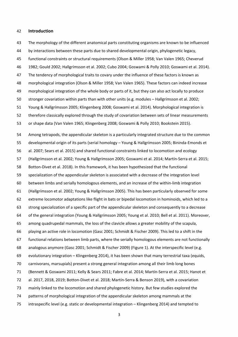
Figure 1: Graphic model showing the hypotheses of morphological integration tested in this study on the 836
appendicular skeleton of the five modern rhino species. Hu: Humerus; Ra: Radius; Ul: Ulna; Fe: Femur; Ti: 837
Tibia; Fi: Fibula. 838
839
840
Figure 2: Plots of the first PLS axes computed on raw shapes. A: humerus-radius; B: humerus-ulna; C: 841
humerus-femur; D: humerus-tibia; E: humerus-fibula; F: radius-ulna; G: radius-femur. rPLS: value of the 842
PLS coefficient; % EC: percentage of explained covariation; Corr. p-value: corrected p-value using a 843
Benjamini-Hochberg correction. The phylogenetic tree displays a polytomy because of the absence of 844
consensus regarding the relationships of the five modern rhinos. 845
32
846
847
33
Figure 3: Plots of the first PLS axes computed on raw shapes. A: radius-tibia; B: radius-fibula; C: ulna-848
femur; D: ulna-tibia; E: ulna-fibula; F: femur-tibia; G: femur-fibula; H: tibia-fibula. rPLS: value of the PLS 849
coefficient; % EC: percentage of explained covariation; Corr. p-value: corrected p-value using a 850
Benjamini-Hochberg correction. Colour code as in Figure 2. 851
34
852
853
35
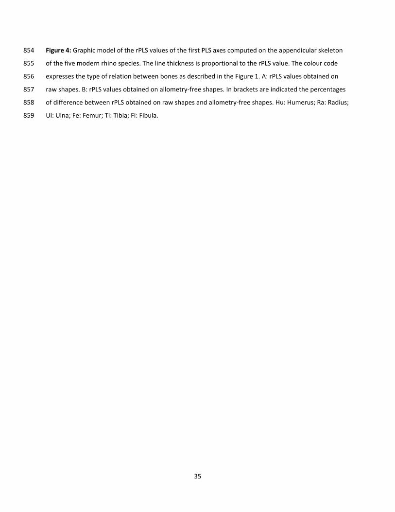
Figure 4: Graphic model of the rPLS values of the first PLS axes computed on the appendicular skeleton 854
of the five modern rhino species. The line thickness is proportional to the rPLS value. The colour code 855
expresses the type of relation between bones as described in the Figure 1. A: rPLS values obtained on 856
raw shapes. B: rPLS values obtained on allometry-free shapes. In brackets are indicated the percentages 857
of difference between rPLS obtained on raw shapes and allometry-free shapes. Hu: Humerus; Ra: Radius; 858
Ul: Ulna; Fe: Femur; Ti: Tibia; Fi: Fibula. 859
36
860
861
37
Figure 5: Colour maps of the location and intensity of the shape deformation associated to the first PLS 862
axes for 4 pairs of bones among the five modern species of rhinoceros. For each bone, the shape 863
associated to the positive part of the first PLS axis was coloured depending on its distance to the shape 864
associated to the negative part (blue indicates a low deformation intensity and red indicates a high 865
deformation intensity). The colour code of the squares expresses the type of relation between bones as 866
described in the Figure 1 (orange: serial homology; blue: functional analogy). A: humerus-femur; B: 867
radius-tibia; C: ulna-fibula; D: humerus-tibia (orientation from left to right in each case: cranial, lateral, 868
caudal and medial). 869
870
38
Figure 6: Colour maps of the location and intensity of the shape deformation associated to the first PLS 871
axes for 4 pairs of bones among the five modern species of rhinoceros. For each bone, the shape 872
associated to the positive part of the first PLS axis was coloured depending on its distance to the shape 873
associated to the negative part (blue indicates a low deformation intensity and red indicate a high 874
deformation intensity). The colour code of the squares expresses the type of relation between bones as 875
described in the Figure 1 (black: intra-limb relation; green: non-homologous or analogous bones). A: 876
radius-ulna; B: femur-tibia; C: tibia-fibula; D: ulna-femur (orientation from left to right in each case: 877
cranial, lateral, caudal and medial). 878
879
880
39
Figure 7: Plots of the first PLS axes computed on allometry-free shapes. A: humerus-radius; B: humerus-881
were previously determined or reattributed based on the analysis of the limb long bone morphology (see 921
Mallet et al. 2019). 922
923
46
Taxon Institution Specimen number Sex Age Condition 3D acquisition Ceratotherium simum AMNH M-51854 F A W SS Ceratotherium simum AMNH M-51855 M A W SS Ceratotherium simum AMNH M-51857 F A W SS Ceratotherium simum AMNH M-51858 M A W SS Ceratotherium simum AMNH M-81815 U A U SS Ceratotherium simum BICPC NH.CON.20 M S W SS Ceratotherium simum BICPC NH.CON.32 F S W SS Ceratotherium simum BICPC NH.CON.40 F S W SS Ceratotherium simum BICPC NH.CON.110 M A W SS Ceratotherium simum BICPC NH.CON.112 M A W SS Ceratotherium simum NHMUK ZD 2018.143 U A U SS Ceratotherium simum NHMW 3086 U A W P Ceratotherium simum RBINS 19904 M S W SS Ceratotherium simum RMCA 1985.32-M-0001 U A W SS Ceratotherium simum RMCA RG35146 M A W SS
Dicerorhinus sumatrensis MNHN ZM-AC-1903-300 M A W SS Dicerorhinus sumatrensis NHMUK ZD 1879.6.14.2 M A W SS Dicerorhinus sumatrensis NHMUK ZD 1894.9.24.1 U A W SS Dicerorhinus sumatrensis NHMUK ZD 1931.5.28.1 M S W SS Dicerorhinus sumatrensis NHMUK ZE 1948.12.20.1 U A U SS Dicerorhinus sumatrensis NHMUK ZE 1949.1.11.1 U A W SS Dicerorhinus sumatrensis NHMW 3082 U A U P Dicerorhinus sumatrensis RBINS 1204 M A W SS Dicerorhinus sumatrensis ZSM 1908/571 M A U SS
Diceros bicornis AMNH M-81805 U A U SS Diceros bicornis AMNH M-27757 M S W SS Diceros bicornis AMNH M-113776 U A W SS Diceros bicornis AMNH M-113777 U A W SS Diceros bicornis AMNH M-113778 U A W SS Diceros bicornis MNHN ZM-AC-1936-644 F S U SS Diceros bicornis RBINS 9714 F A W SS Diceros bicornis RMCA RG2133 M S W SS Diceros bicornis ZSM 1961/186 M S U SS Diceros bicornis ZSM 1961/187 M S U SS
Rhinoceros sondaicus CCEC 50002041 U A W SS Rhinoceros sondaicus MNHN ZM-AC-A7970 U A U SS Rhinoceros sondaicus MNHN ZM-AC-A7971 U A W SS Rhinoceros sondaicus NHMUK ZD 1861.3.11.1 U S W SS Rhinoceros sondaicus NHMUK ZD 1871.12.29.7 M A W SS Rhinoceros sondaicus NHMUK ZD 1921.5.15.1 F S W SS Rhinoceros sondaicus RBINS 1205F U S W SS Rhinoceros unicornis AMNH M-35759 M A C SS Rhinoceros unicornis AMNH M-54456 F A W SS Rhinoceros unicornis MNHN ZM-AC-1960-59 M A C SS Rhinoceros unicornis NHMUK ZD 1884.1.22.1.2 F A W SS Rhinoceros unicornis NHMUK ZE 1950.10.18.5 M A W SS Rhinoceros unicornis NHMUK ZE 1961.5.10.1 M A W SS Rhinoceros unicornis NHMUK ZD 1972.822 U A U SS Rhinoceros unicornis RBINS 1208 F A C SS Rhinoceros unicornis RBINS 33382 U A U SS
924
47
Table 2: Values of the rPLS for the first PLS axes for each of the five species, with respective p-values before (p) and after (p cor.) the Benjamini-925
Hochberg correction. Values in bold are the statistically significant ones (p or p cor. < 0.05). Abbreviations: Hum: Humerus: Rad: Radius; Uln: 926
Ulna; Fem: Femur; Tib: Tibia; Fib: Fibula. 927
C. simum (n=15) Ds. sumatrensis (n=9) Dc. bicornis (n=10) R. sondaicus (n=7) R. unicornis (n=9)
for the talus; Ca.l.: Caudo-lateral line; Ca.t.l.m.: Caudal tubercle of the lateral malleolus; Cr.l.: Cranio-958
lateral line; Cr.t.l.m.: Cranial tubercle of the lateral malleolus; D.a.s.t.: Distal articular surface for the 959
tibia; D.g.m.: Distal groove of the malleolus; H.: Head; I.c.: Interosseous crest; L.g.: Lateral groove; 960
P.a.s.t.: Proximal articular surface for the tibia. 961
962
49
963
50
Data S2: Designation and location of the anatomical landmarks placed on each bone. 964
965
Bone Anatomical LM Curve sliding semi-LM Surface sliding semi-LM Total Humerus 35 639 559 1233
Radius 23 393 493 909 Ulna 21 343 540 904
Femur 27 612 518 1157 Tibia 24 384 540 948
Fibula 12 269 454 735 966
Table S2A: Total number of anatomical landmarks (LM), curve sliding and surface sliding semi-967
landmarks for each bone. 968
969
51
LM Designation 1 Most distal point of the lateral border of the bicipital groove 2 Most proximal point of the lateral border of the bicipital groove 3 Most proximal point of the intermediate tubercle 4 Most proximal point of the medial border of the bicipital groove 5 Most distal point of the medial border of the bicipital groove 6 Most distal point of the intermediate tubercle 7 Most medial point of the top of the lesser tubercle 8 Most cranial point of the lesser tubercle convexity 9 Most medio-caudal point of the lesser tubercle convexity
10 Most medial point of the humeral head surface 11 Most caudo-distal point of the humeral head surface 12 Contact point between the tricipital line and the caudal border of the articular head surface 13 Most lateral point of the humeral head surface 14 Most caudal point of the greater tubercle convexity 15 Most proximal point of the greater tubercle convexity 16 Most cranial point of the greater tubercle convexity crest 17 Most proximal point of the m. infraspinatus lateral insertion 18 Most distal point of the m. infraspinatus lateral insertion 19 Most proximal point of the deltoid tuberosity 20 Most distal point of the deltoid tuberosity 21 Most proximal point of the epicondylar crest tuberosity 22 Most distal point of the epicondylar crest tuberosity 23 Most lateral point of the lateral epicondyle 24 Most distal point of the lateral epicondyle 25 Most proximo-lateral point of the capitulum 26 Most cranio-proximal point of contact between the trochlea and the capitulum 27 Most cranial point of the trochlea groove 28 Most cranio-medial point of the dorsal side of the trochlea
29 Most distal contact point between the trochlea border and the medial development of the trochlea lip
30 Most cranio-medial point of the ventral side of the trochlea 31 Most cranio-lateral point of the ventral side of the trochlea 32 Most caudo-distal point of contact between the capitulum and the trochlea 33 Most medial point of the medial epicondyle 34 Most caudal point of the medial epicondyle 35 Most lateral point of the medial epicondyle
970
Table S2B: Designation of the anatomical landmarks on the humerus.971
52
Figure S2C: Location of the anatomical landmarks (red spheres), curve sliding (blue spheres) and surface sliding (green spheres) semi-landmarks placed on
the humerus. From left to right: caudal, lateral, cranial and medial views. Numbers refer to anatomical landmarks designation detailed in Table S1B.
53
LM Designation 1 Most caudo-lateral point of the lateral glenoid cavity 2 Most cranio-lateral point of the lateral glenoid cavity 3 Tip of the coronoid process 4 Most cranial point of the medial glenoid cavity 5 Most caudo-medial point of the medial glenoid cavity 6 Tip of the palmar process of the glenoid cavity ridge 7 Most cranial point of the lateral insertion relief 8 Most lateral point of the lateral insertion relief 9 Most caudo-distal point of the proximo-lateral articular facet for the ulna
10 Most caudo-distal point of the proximo-medial articular facet for the ulna 11 Most proximal point of the interosseous crest (= most distal point of the interosseous space) 12 Most distal point of the interosseous crest (crossing the distal epiphysis line) 13 Most cranio-lateral point of the disto-lateral articulation surface for ulna 14 Most proximo-lateral point of the disto-lateral articulation surface for ulna 15 Most caudo-lateral point of the disto-lateral articulation surface for ulna 16 Most medial point of the transversal crest 17 Tip of the radial styloid process 18 Maximum of curvature of the cranial ridge of the articular facet for the scaphoid 19 Most cranio-lateral point of the articular facet for the scaphoid 20 Most lateral point of the articular facet for the semilunar 21 Most caudo-lateral point of the articular facet for the semilunar 22 Most caudo-lateral point of the articular facet for the scaphoid 23 Most cranio-proximal point of the medial facet of distal radius
Table S2D: Designation of the anatomical landmarks on the radius.
54
Figure S2E: Location of the anatomical landmarks (red spheres), curve sliding (blue spheres) and surface sliding (green spheres) semi-landmarks placed on
the radius. From left to right: caudal, lateral, cranial and medial views. Numbers refer to anatomical landmarks designation detailed in Table S1D.
55
LM Designation 1 Most proximo-cranial point of the olecranon tuberosity cranial border 2 Most lateral point of the olecranon tuberosity 3 Most caudo-distal point of the olecranon tuberosity 4 Most medial point of the olecranon tuberosity 5 Most proximal point of the olecranon tuberosity 6 Cranial tip of the anconeal process 7 Most distal point of the lateral part of the trochlear notch articular surface 8 Maximum concavity point of the distal border of the trochlear notch articular surface 9 Most distal point of the medial part of the trochlear notch articular surface
10 Most distal point of the proximo-medial articular facet for the radius 11 Most distal point of the proximo-lateral articular facet for the radius
12 Most distal point of the proximal synostosis surface for the radius (= most proximal point of the interosseous space)
13 Most medio-caudal point of the distal radio-ulnar synostosis surface 14 Most disto-medial point of the articular surface with the semilunar bone 15 Most cranio-lateral point of the articular surface with the semilunar bone 16 Most disto-lateral point of the articular surface with the semilunar bone 17 Most cranio-lateral point of the distal radio-ulnar synostosis surface 18 Most lateral point of the distal epiphysis 19 Caudo-distal tip of ulnar styloid process
20 Most proximal contact point between the articular surfaces for the pisiform and the triquetrum
21 Most distal contact point between the caudal border of the ulna and the articular surface with the pisiform
Table S2F: Designation of the anatomical landmarks on the ulna.
56
Figure S2G: Location of the anatomical landmarks (red spheres), curve sliding (blue spheres) and surface sliding (green spheres) semi-landmarks placed on
the ulna. From left to right: caudal, lateral, cranial and medial views. Numbers refer to anatomical landmarks designation detailed in Table S1F.
57
LM Designation 1 Most proximo-cranial point of the greater trochanter 2 Most proximo-caudal point of the greater trochanter 3 Most medial point of the greater trochanter convexity 4 Most distal point of the intertrochanteric crest 5 Most disto-caudal point of the greater trochanter 6 Most cranio-lateral point of the convexity of the greater trochanter
7 Most proximal contact point between the intertrochanteric line and the medial line of the cranial face
8 Most lateral point of the border of the head 9 Most proximal point of the lesser trochanter
10 Most distal point of the lesser trochanter 11 Most proximal point of the gluteal tuberosity on the third trochanter 12 Most distal point of the gluteal tuberosity on the third trochanter 13 Most medial point of the medial epicondyle 14 Contact point between the intercondylar line and the medial condyle 15 Contact point between the intercondylar line and the lateral condyle 16 Most lateral point of the lateral epicondyle 17 Most proximal point of the lateral lip of the trochlea 18 Most proximal point of the trochlear groove 19 Most proximal point of the medial lip of the trochlea 20 Most distal point of the medial lip of the trochlea 21 Distal maximum of curvature of the trochlear groove 22 Most distal point of the lateral lip of the trochlea 23 Most medial point of the fossa extensoria 24 Most lateral point of the fossa extensoria 25 Most cranial point of the fossa extensoria 26 Most proximo-medial point of the lateral condyle articular surface 27 Most proximo-lateral point of the medial condyle articular surface
Table S2H: Designation of the anatomical landmarks on the femur.
58
Figure S2I: Location of the anatomical landmarks (red spheres), curve sliding (blue spheres) and surface sliding (green spheres) semi-landmarks placed on
the femur. From left to right: caudal, lateral, cranial and medial views. Numbers refer to anatomical landmarks designation detailed in Table S1H. Landmark
n°26 situated in the intercondylar space cannot be seen.
59
LM Designation 1 Most proximal point of the lateral tubercle of the intercondylar eminence 2 Most proximo-cranial point of the lateral tubercle of the intercondylar eminence 3 Most cranial point of the articular surface of the lateral condyle 4 Most caudal point of the articular surface of the lateral condyle 5 Most caudal point of the lateral tubercle of the intercondylar eminence 6 Most caudo-proximal point of the medial tubercle of the intercondylar eminence 7 Most proximal point of the medial tubercle of the intercondylar eminence 8 Most cranial point of the articular surface of the medial condyle 9 Most caudal point of the articular surface of the medial condyle
10 Most proximal point of the proximal tibio-fibular synostosis surface 11 Most distal point of the proximal tibio-fibular synostosis surface 12 Most proximal point of the lateral part of the tibial tuberosity 13 Most distal point of the lateral part of the tibial tuberosity 14 Most distal point of the tibial tuberosity groove 15 Most proximal point of the medial part of the tibial tuberosity 16 Most caudal point of the medial condyle 17 Most proximal point of the distal tibio-fibular synostosis surface 18 Most caudo-lateral point of the distal articular surface 19 Most cranio-lateral point of the distal articular surface 20 Most cranio-distal point of the intermediate ridge of the distal articular surface 21 Most distal point of the contact between the medial malleolus and the distal articular surface 22 Most distal point of the medial part of the distal articular surface 23 Most caudo-distal point of the intermediate ridge of the distal articular surface 24 Most medial point of the medial malleolus
Table S2J: Designation of the anatomical landmarks on the tibia.
60
Figure S2K: Location of the anatomical landmarks (red spheres), curve sliding (blue spheres) and surface sliding (green spheres) semi-landmarks placed on
the tibia. From left to right: caudal, lateral, cranial and medial views. Numbers refer to anatomical landmarks designation detailed in Table S1J.
61
LM Designation 1 Most proximal point of the proximal tibio-fibular synostosis surface 2 Most caudo-medial point of the proximal tibio-fibular synostosis surface 3 Most cranio-lateral point of the proximal tibio-fibular synostosis surface 4 Most proximal point of the distal tibio-fibular synostosis surface 5 Most caudal point of the distal articular facet 6 Most distal point of the caudal part of the distal articular facet 7 Most distal point of the cranial part of the distal articular facet 8 Most cranial point of the distal articular facet 9 Distal tip of the caudal ridge of the lateral malleolar sulcus
10 Distal tip of the cranial ridge of the lateral malleolar sulcus 11 Most lateral point of the cranial ridge of the lateral malleolar sulcus 12 Most disto-medial point of the proximal epiphysis = end of the latero-caudal crest
Table S2L: Designation of the anatomical landmarks on the fibula.0
62
1
Figure S2M: Location of the anatomical landmarks (red spheres), curve sliding (blue spheres) and surface sliding (green spheres) semi-landmarks 2
placed on the fibula. From left to right: caudal, lateral, cranial and medial views. Numbers refer to anatomical landmarks designation detailed in 3
Table S1L.4
63
Figure S3: Plots of the second PLS axes computed on raw shapes. A: humerus-radius; B: humerus-ulna; C: 5
rPLS: value of the PLS coefficient; % EC: percentage of explained covariation; Corr. p-value: corrected p-8
value using a Benjamini-Hochberg correction. 9
64
10
65
Figure S4: Shape deformations associated with the first PLS axes for the fifteen bone pairs. Blue: negative side of the axis. Orange: positive side of 11
the axis. The colour code of the squares expresses the type of relation between bones as described in the Figure 1 (black: intra-limb relation; 12
orange: serial homology; blue: functional analogy; green: non-homologous or analogous bones). A: humerus-radius; B: humerus-ulna; C: radius-13
E: ulna-tibia; F: humerus-fibula; G: radius-femur (orientation from left to right in each case: cranial, 24
lateral, caudal and medial). 25
26
67
27
28
68
Figure S6: Shape deformations associated with the first PLS axes for the fifteen bone pairs. Blue: negative side of the axis. Orange: positive side of 29
the axis. The colour code of the squares expresses the type of relation between bones as described in the Figure 1 (black: intra-limb relation; 30
orange: serial homology; blue: functional analogy; green: non-homologous or analogous bones). A: humerus-radius; B: humerus-ulna; C: radius-31