University of Mississippi University of Mississippi

eGrove eGrove

Electronic Theses and Dissertations Graduate School

2018

A Framework For Assessing Water Quality, Prioritizing Recovery A Framework For Assessing Water Quality, Prioritizing Recovery

Potential, And Analyzing Placement Of Best Management Potential, And Analyzing Placement Of Best Management

Practices Practices

Tadesse Animaw Sinshaw University of Mississippi

Follow this and additional works at: https://egrove.olemiss.edu/etd

Part of the Environmental Engineering Commons

Recommended Citation Recommended Citation Sinshaw, Tadesse Animaw, "A Framework For Assessing Water Quality, Prioritizing Recovery Potential, And Analyzing Placement Of Best Management Practices" (2018). Electronic Theses and Dissertations. 940. https://egrove.olemiss.edu/etd/940

This Dissertation is brought to you for free and open access by the Graduate School at eGrove. It has been accepted for inclusion in Electronic Theses and Dissertations by an authorized administrator of eGrove. For more information, please contact egrove@olemiss.edu.

A FRAMEWORK FOR ASSESSING WATER QUALITY, PRIORITIZING RECOVERY

POTENTIAL, AND ANALYZING PLACEMENT OF BEST MANAGEMENT

PRACTICES

A dissertation presented

in partial fulfillment of the requirements

for the

Doctor of Philosophy Degree

in Engineering Science

Emphasis in Environmental Engineering

Tadesse Animaw Sinshaw

Department of Civil Engineering

University of Mississippi

May 2018

Copyright © 2018 by Tadesse Animaw Sinshaw

All rights reserve

ii

ABSTRACT

Motivated by the U.S. EPA goals, this research developed a framework to support

identification and restoration of nutrient-impaired water bodies. The study objectives were

developing total nitrogen (TN) and total phosphorus (TP) prediction models, evaluating the impact

of social indicators on assessing recovery potential, and developing a spatial decision support

system for choice and placement of best management practices (BMPs). An artificial neural

network was used to develop TN and TP predictive regional models for U.S. lakes using easily

measurable and cost-effective variables. The performance of models was superior for regions

trained with larger datasets and/or regions with lower temperature and precipitation variability.

The use of datasets larger than existing records and obtained from homogeneous climatic region

was suggested to achieve the desired performance. The impact of social indicators on assessing a

recovery potential was studied by comparing four watersheds using ecological, stressor, and social

indicators. Social indicators were grouped into Socio-Economic, Organizational, and Information

and Planning subcategories. The existing U.S. EPA Recovery Potential Screening tool prioritizes

restoration for a water body with the most favorable ecological and social condition as well as the

least stressing factors. In the present study, water bodies ranked lowest were observed with lower

social scores associated with lower Socio-Economic conditions. This could mean a manager would

take a water body with lower Socio-Economic condition as the lowest priority for restoration. It is

suggested that such prioritization plan should carefully incorporate community goals in a

prioritization effort because restoration supports an improvement of quality of life. A spatial

decision support system was developed with the necessary information to assess nitrogen (N)

iii

pollution and methods to estimate an annual exported N load into Beasley Lake, Mississippi. A

decision analysis of choice and placement of BMPs was performed based on performance, site

suitability, and establishment cost criteria. From this analysis, a BMP scenario that reduces 25%

of the exported load at an establishment and an annual opportunity cost-to-performance ratios of

148 $/kg and 29 $/kg, respectively, was developed. The presented approach supports similar

efforts when the use of existing watershed models is limited by data availability.

iv

DEDICATION

This work is dedicated to my parents, Animaw Sinshaw and Tsehayneshi Taye, and my

wife, Yalemzerf Belete, who have been a constant source of support and encouragements during

the challenges of this work.

v

LIST OF ABBREVIATIONS

A Area

AD Atmospheric Deposition

AL Atmospheric Loss

ANOVA Analysis of Variance

ARS Agricultural Research Service

ASE Average of Squared Error

BLW Beasley Lake Watershed

BMP Best Management Practice

CH Crop Harvest

cm Centimeter

CP Conservation Practice

CRP Conservation Reserve Program

Da Drainage Area

DAR Drainage Area Ratio

DEM Digital Elevation Model

EPA Environmental Protection Agency

F Fertilizer

FL Fixation by Legumes

FromElev From Elevation

vi

GIS Geographical Information System

GW Ground Water

H Hidden

ha Hectare

HN Hidden Node

HUC Hydrologic Unit Code

I Input

IRP Integrated Recovery Potential

K Decay Coefficient

Km kilometer

l Liter

L Livestock

LIDAR Light Detection and Ranging

Log Logarithm

m Meter

MARE Mean Absolute Relative Error

Max Maximum

MCDA Multi-Criteria Decision Analysis

MDEQ Mississippi Department of Environmental Quality

MDMESA Mississippi Delta Management Systems Evaluation Area

mg Milligram

Min Minimum

mm Millimeter

vii

MS Mississippi

N Nitrogen

NADP National Atmospheric Deposition Program

No. Number

NTU Nephelometric Turbidity Unit

O Output

oC

ΔP

Degree Centigrade

Precipitation difference

P Phosphorus

PPM Parts Per Million

Q Discharge

QOL Quality of Life

R Region

R2 Coefficient of Determination

RPI Recovery Potential Index

RPS Recovery Potential Screening

s Segment Slope

S Soil Potential Maximum Retention

SCS Soil Conservation Service

SDSS Spatial Decision Support System

SI Sensitivity Index

SSURGO

ΔT

Soil Survey Geographic Database

Temperature difference

viii

T Time

TMDL Total Maximum Daily Load

TN Total Nitrogen

ToElev To Elevation

TP Total Phosphorus

TT Trapped by Trees

U.S. United States

USDA United States Department of Agriculture

USGS United States Geological Survey

V Velocity

WQS Water Quality Standard

Y Year

µg Microgram

µs Micro-Siemens

3D Three-dimensional

ix

ACKNOWLEDGMENT

I am very grateful to many people who supported me throughout this work. My deepest

appreciation goes to my Ph.D. advisor, Dr. Cristiane Queiroz Surbeck. I am fortunate to have Dr.

Surbeck’s guidance and support in my years at the University of Mississippi. I have been given all

the advice required by a student. She has been patient during those times I struggled to find

direction and encouraged me when I move forward. She is incredibly generous with her time,

always making time for me in her schedule for academic and career advice. I have learned much

from her advice.

I am also thankful to my dissertation committee members, Dr. Yacoub Najjar, Dr. Douglas

Shields, and Dr. Marjorie M. Holland for their research advice. They enriched my research

experience and this dissertation is better as a result of their help. I appreciate Dr. Shields’s role for

connecting me with the USDA Sedimentation Laboratory at Oxford, Mississippi, which created

opportunities to access data and get technical advice. I would additionally like to acknowledge Dr.

Lindsey Yasarer of the USDA Sedimentation Laboratory for her crucial guidance and data access.

I also would like to thank Dr. Azad Hossain for co-advising the third phase of this dissertation. I

also acknowledge the financial support provided by the McLean Institute for Public Service and

Community Engagement at the University of Mississippi through a grant from the Robert M.

Hearin Support Foundation.

I am also deeply thankful to those of family members who supported me in every aspect.

My special thanks go to my father, Animaw Sinshaw and my mother, Tsehaynesh Taye for their

endless love and encouragement. I thank my wife, Yalemzerf Belete, for her love and support

x

throughout the completion of this dissertation. It would not have been a reality without her. The

time she spent caring for our household provided me a chance to move this dissertation to

completion. I also would like to thank my brothers, Muluken, Temesgen, Fiseha, and Abay, for

their support and encouragement throughout my study time. I also appreciate all of those, not

mentioned here, who provided me tremendous support in this work.

xi

TABLE OF CONTENTS

ABSTRACT .................................................................................................................................... ii

DEDICATION ............................................................................................................................... iv

LIST OF ABBREVIATIONS ......................................................................................................... v

ACKNOWLEDGMENT................................................................................................................ ix

LIST OF TABLES ........................................................................................................................ xv

LIST OF FIGURES .................................................................................................................... xvii

CHAPTER Ι .................................................................................................................................... 1

INTRODUCTION .......................................................................................................................... 1

1.1 BACKGROUND .................................................................................................................. 2

1.2 RESEARCH NEEDS ............................................................................................................ 4

1.5 ORGANIZATION OF THE DISSERTATION.................................................................... 7

LIST OF REFERENCES ................................................................................................................ 8

CHAPTER ΙΙ ................................................................................................................................. 10

APPLICATION OF ARTIFICIAL NEURAL NETWORKS FOR PREDICTION OF TOTAL

NITROGEN AND TOTAL PHOSPHORUS IN U.S. LAKES .................................................... 10

2.1 INTRODUCTION .............................................................................................................. 12

2.2 BACKGROUND ................................................................................................................ 15

2.2.1 Basics of Artificial Neural Network ............................................................................ 15

2.2.2 Artificial Neural Networks in the Environmental Field .............................................. 18

xii

2.3 METHODOLOGY ............................................................................................................. 21

2.3.1 Description of Training Datasets ................................................................................. 21

2.3.2 Choice of Network Input Variables ............................................................................. 22

2.3.3 Data Normalization ...................................................................................................... 23

2.3.4 Development of the ANN Model ................................................................................. 23

2.3.5 Development of Linear Regression Model .................................................................. 26

2.3.6 Sensitivity Analysis ..................................................................................................... 27

2.3.7 Excel Application......................................................................................................... 27

2.4 RESULTS AND DISCUSSION ......................................................................................... 29

2.4.1 Results from the Choice of Network Input Variables .................................................. 29

2.4.2 Results from the ANN Model ...................................................................................... 31

2.4.3. Results from the Regression Model ............................................................................ 39

2.4.4 Results from the Sensitivity Analysis .......................................................................... 41

2.5 CONCLUSIONS................................................................................................................. 43

LIST OF REFERENCES .......................................................................................................... 45

APPENDIX ............................................................................................................................... 49

CHAPTER ΙΙΙ ............................................................................................................................... 92

ABSTRACT .............................................................................................................................. 93

3.1 INTRODUCTION .............................................................................................................. 94

3.2 BACKGROUND ................................................................................................................ 96

3.3 STUDY AREA ................................................................................................................. 100

xiii

3.4 METHODS ....................................................................................................................... 102

3.4.1 Indicator Selection and Measurement ........................................................................ 102

3.4.2 Development of the Sensitivity Analysis Model ....................................................... 107

3.4.3 Sensitivity Analysis on the Four Priority Watersheds ............................................... 108

3.5 RESULTS AND DISCUSSION ....................................................................................... 110

3.5.1 Initial Results using the U.S. EPA-RPS Tool ............................................................ 110

3.5.2. Evaluation of Indices for Four Priority Watersheds ................................................. 111

3.5.3 “What If” Sensitivity Analysis................................................................................... 114

3.6 CONCLUSIONS............................................................................................................... 119

LIST OF REFERENCES ........................................................................................................ 121

CHAPTER ΙV ............................................................................................................................. 126

APPLICATION OF A SPATIAL DECISION SUPPORT SYSTEM FOR CHOICE AND

PLACEMENT OF NITROGEN SOURCE REDUCING BEST MANAGEMENT PRACTICES

IN THE BEASLEY LAKE WATERSHED ............................................................................... 126

ABSTRACT ............................................................................................................................ 127

4.1 INTRODUCTION ............................................................................................................ 128

4.2 STUDY AREA ................................................................................................................. 131

4.3 RESEARCH OBJECTIVE ............................................................................................... 133

4.4 METHODOLOGY ........................................................................................................... 134

4.4.1 Analytical Model ....................................................................................................... 134

4.4.2 Database Pool............................................................................................................. 146

xiv

4.4.4 Spatial Decision Analysis .......................................................................................... 152

4.5 RESULTS AND DISCUSSION ....................................................................................... 156

4.5.1 Stream and Sub-basin Delineation ............................................................................. 156

4.5.2 Unit Area N Yield Estimation.................................................................................... 157

4.5.3 In-stream Exported N Load Estimation ..................................................................... 160

4.5.4 Results from the Spatial Decision Analysis ............................................................... 162

4.6 CONCLUSIONS............................................................................................................... 169

LIST OF REFERENCES ........................................................................................................ 171

CHAPTER V .............................................................................................................................. 176

CONCLUSIONS......................................................................................................................... 176

5.1 OVERVIEW OF FINDINGS ........................................................................................... 177

5.2. LIMITATIONS OF THE PRESENT STUDIES ............................................................. 180

5.3 RECOMMENDATIONS FOR FUTURE STUDIES ....................................................... 182

VITA ........................................................................................................................................... 184

xv

LIST OF TABLES

Table 1. A summary of assessed waters in the U.S. ....................................................................... 3

Table 2. Correlation coefficient (R) matrix of selected network variables. .................................. 30

Table 3. Descriptive statistics of selected network variables. ...................................................... 30

Table 4. Optimized model parameters for national and regional networks. ................................. 35

Table 5. Regional variability characteristics of the summer season datasets. .............................. 37

Table 6. Regional variability factors. ............................................................................................ 38

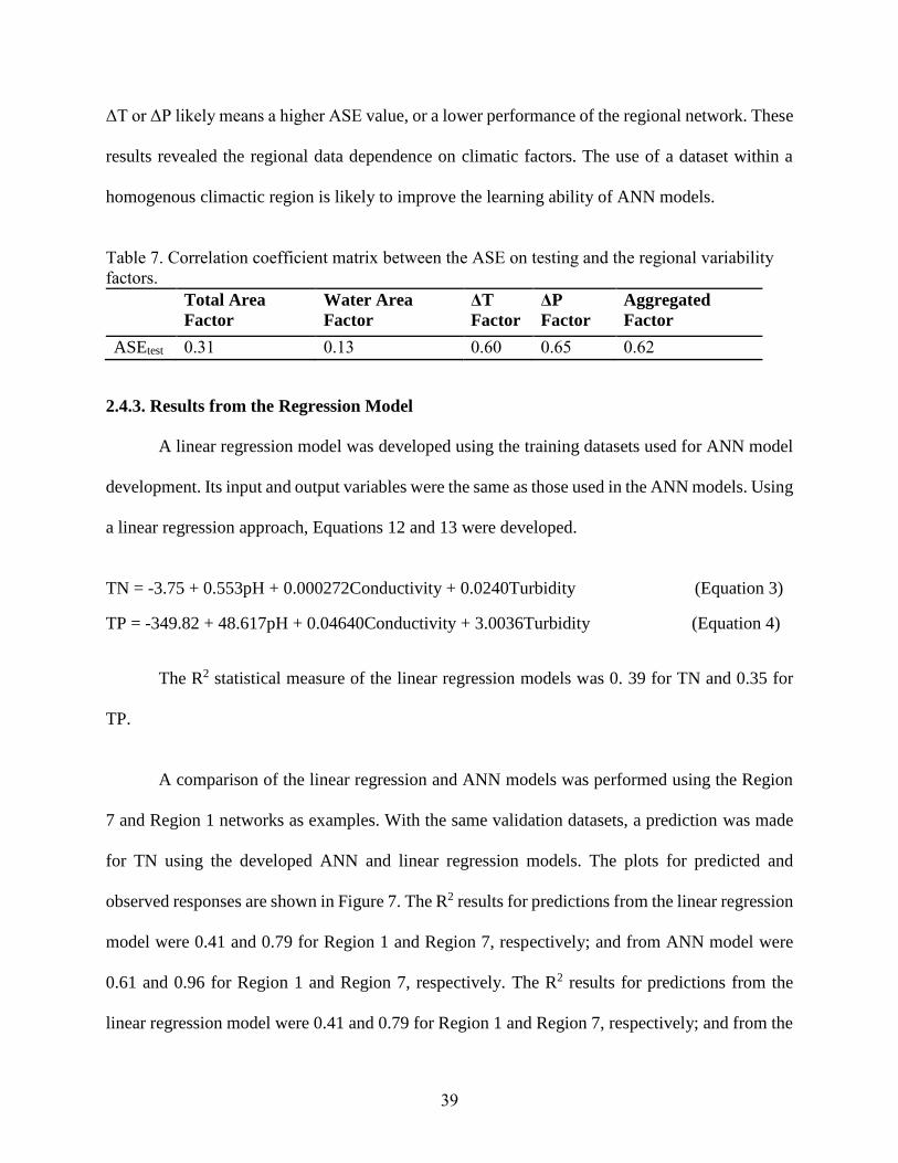
Table 7. Correlation coefficient matrix between the ASE on testing and the regional variability

factors. ................................................................................................................................... 39

Table 8. Sensitivity index values of network outputs to input variables. ..................................... 42

Table 9. Examples of measured indicators under the U.S. EPA NLA program. .......................... 50

Table 10. Measured data for selected network variables. ............................................................. 51

Table 11 Hydrological, geographical, and demographic characteristics of the studied water

bodiesa. ................................................................................................................................ 102

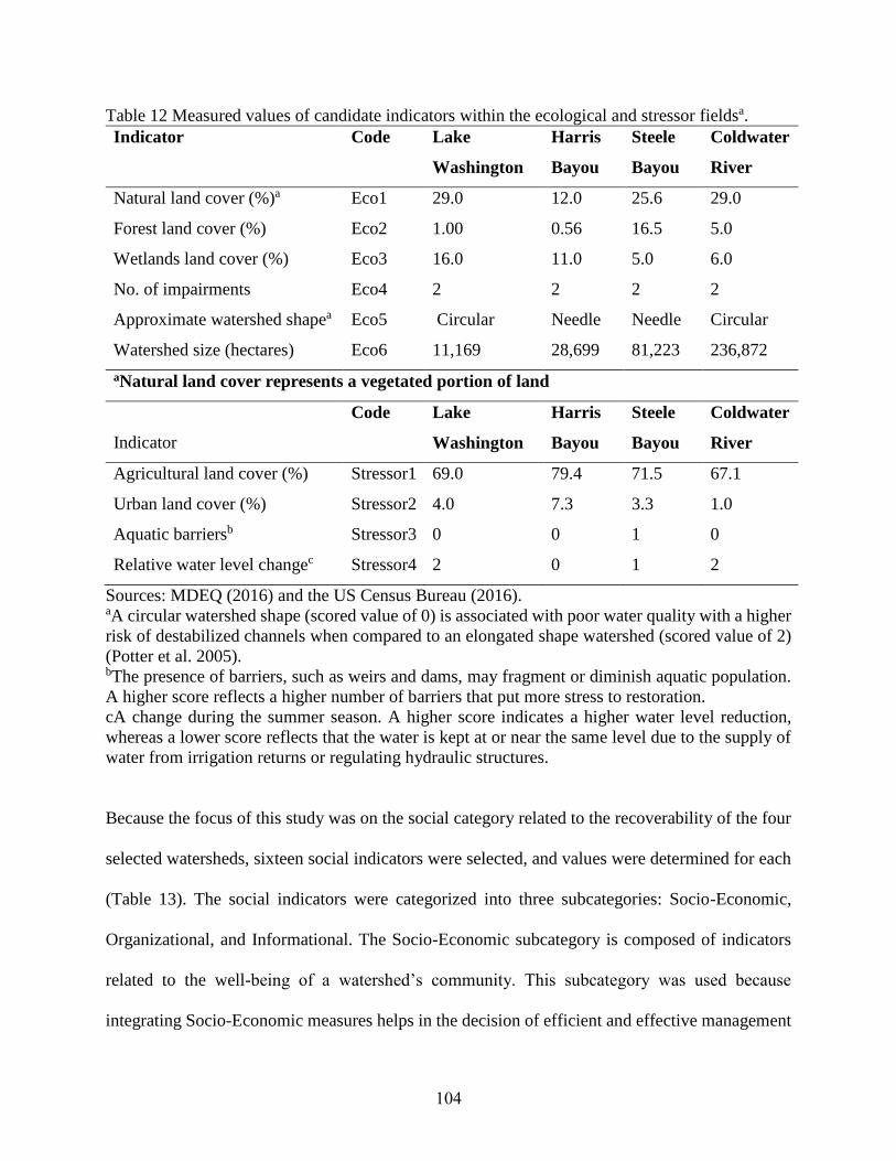
Table 12 Measured values of candidate indicators within the ecological and stressor fieldsa. .. 104

Table 13. Measured values of candidate indicators within the social fielda. .............................. 106

Table 14. List of data sets stored in the database pool................................................................ 146

Table 15. Description of selected BMPs..................................................................................... 154

Table 16. Description of evaluated BMP scenarios. ................................................................... 155

Table 17. Component estimates for Beasley Lake Watershed from cropland N budget. ........... 158

Table 18. Estimated cost for establishing BMP scenarios. ......................................................... 167

xvi

Table 19. Comparison of BMP scenarios. .................................................................................. 168

xvii

LIST OF FIGURES

Figure 1. The Clean Water Act regulatory structure for water quality management in the U.S.

(U.S. EPA 2016). .................................................................................................................... 3

Figure 2. Lake monitoring sites of the U.S. EPA-NARS (reprinted from U.S. EPA, 2013). The

blue dots represent the natural lakes, and the brown dots indicate the man-made reservoirs.

............................................................................................................................................... 22

Figure 3. A screenshot of the Excel application of regional networks. ........................................ 28

Figure 4. Log-distributions of training datasets. TP is total phosphorus; TN is total nitrogen (data

from U.S. EPA 2013). ........................................................................................................... 31

Figure 5. The structure of a feed-forward back-propagation neural network for pH, conductivity,

and turbidity nodes in the input layer, and TP and TN nodes in the output layer. ............... 32

Figure 6. U.S. EPA regional map (modified from U.S. EPA 2016f). R represents the U.S. EPA

region and numbers in each region indicate the size of datasets. ......................................... 33

Figure 7. Prediction accuracy for linear regression and ANN models using the 2007 datasets. .. 41

Figure 8. Prediction accuracy of Regional ANN model using the 2012 U.S. EPA National Lake

Assessment data. ................................................................................................................... 41

Figure 9. Sensitivity results of outputs TN and TP to inputs pH, conductivity, and turbidity using

Region 1 as an example. ....................................................................................................... 42

Figure 10. Watershed boundaries of the four studied water bodies in the Delta region of

Mississippi. ......................................................................................................................... 101

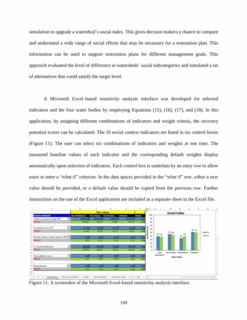
Figure 11. A screenshot of the Microsoft Excel-based sensitivity analysis interface. ............... 109

xviii

Figure 12. Screened watersheds in the state of Mississippi. ....................................................... 111

Figure 13. Index scores of social, ecological, and stressor fields based on the baseline data. ... 112

Figure 14. Examples of “what it takes” simulations applied to the social index of the lowest-

ranked water body, Steele Bayou. ....................................................................................... 117

Figure 15. Location and land use of the Beasley Lake Watershed. ............................................ 132

Figure 16. Digital Elevation Model of the Beasley Lake Watershed. ........................................ 136

Figure 17. A 3D surface representation of the Beasley Lake Watershed. .................................. 137

Figure 18. Known flow lines in the Beasley Lake Watershed. ................................................... 138

Figure 19. Stream networks of the Beasley Lake Watershed. .................................................... 139

Figure 20. Sub-basins of the Beasley Lake Watershed. .............................................................. 140

Figure 21. Location of the existing BMPs in the Beasley Lake Watershed (2005).................... 141

Figure 22. An index gauged site for the Beasley Lake Watershed. ............................................ 145

Figure 23. LIDAR data covering the Beasley Lake Watershed area (USGS). ........................... 147

Figure 24. Hydrography of the Beasley Lake Watershed (processed from USGS NHDPlus

version 2). ........................................................................................................................... 148

Figure 25. Hydrological soil map of the Beasley Lake Watershed. ........................................... 150

Figure 26. The modeling framework for nitrogen assessment. .................................................. 151

Figure 27. Hydrologic network of streams and sub-basins of the Beasley Lake Watershed. ..... 157

Figure 28. Land use and main drainage lines of the Beasley Lake Watershed. ......................... 158

Figure 29. Unit area N yield of the Beasley Lake Watershed. ................................................... 160

Figure 30. N load exported in-stream along flow pathways. ...................................................... 161

xix

Figure 31. Critical watershed sites of the Beasley Lake Watershed. .......................................... 163

Figure 32. Suitable sites for establishment of buffer in the Beasley Lake Watershed. .............. 164

Figure 33. An export coefficient for stream reaches in the Beasley Lake Watershed. ............... 165

Figure 34. Spatial allocation of BMP scenarios in the Beasley Lake Watershed. ...................... 166

1

CHAPTER Ι

INTRODUCTION

2

1.1 BACKGROUND

Nutrient pollution, mainly by excess nitrogen (N) and phosphorus (P), is one of the most

common types of water quality problems. N and P are primary nutrients in water required by algae

and aquatic plants and are also a source of food and habitat for aquatic organisms. However, the

presence of excess N and P in the water leads to excess growth of algae. The decomposition of

excess algae can severely reduce the dissolved oxygen in the water and cause eutrophication,

which is harmful to fish and aquatic life (Portielje and Van der Molen 1999; U.S. EPA 2017b).

The U.S. EPA identified nutrient pollution as the most widespread water quality problem

in the U.S. About 50% of streams and 45% of assessed lakes in the U.S. are identified to be in fair

to poor conditions for N and P concentrations (U.S. EPA 2013). Water bodies that do not meet

water quality standards or designated use criteria for N and P are listed as nutrient-impaired water

bodies under the Clean Water Act Section 303(d). Nutrients are identified as the third general

cause of impairments in assessed rivers and streams and the second general cause of impairments

in assessed lakes, reservoirs, and ponds (U.S. EPA 2017a).

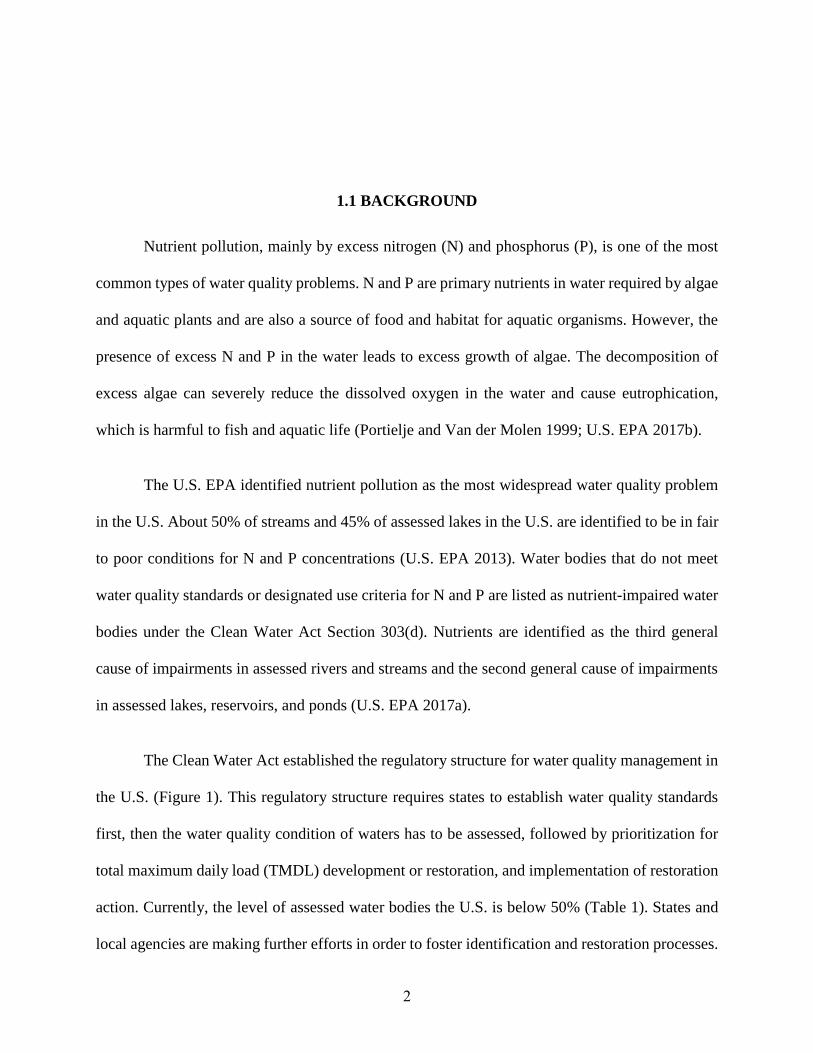
The Clean Water Act established the regulatory structure for water quality management in

the U.S. (Figure 1). This regulatory structure requires states to establish water quality standards

first, then the water quality condition of waters has to be assessed, followed by prioritization for

total maximum daily load (TMDL) development or restoration, and implementation of restoration

action. Currently, the level of assessed water bodies the U.S. is below 50% (Table 1). States and

local agencies are making further efforts in order to foster identification and restoration processes.

3

This Ph.D. dissertation is triggered by the key challenges highlighted by the U.S. EPA

related to identification and restoration of impaired waters.

Figure 1. The Clean Water Act regulatory structure for water quality management in the U.S.

(U.S. EPA 2016).

Table 1. A summary of assessed waters in the U.S.

Rivers and Streams

(km)

Lakes, Reservoirs,

and Ponds

(ha)

Bays and

Estuaries (ha)

Total assessed waters 1,789,668 7,621,187 9,089,304

Total waters 5,686,142 16,861,652 22,737,765

Percent of assessed waters 31.5 45.2 40.0

Information summarized in Table 1 is based on water quality data reported by states to EPA

under Section 305(b) and 303(d) of the Clean Water Act (U.S. EPA 2017a).

Establish Water Quality Standards (WQS)

Designated Uses & Water Quality Criteria

Assess Water Quality Condition

Meeting WQS? Yes

303(d) – Impaired/Threatened

Restoration Program

Reduce Pollution Load

No

Prioritize – TMDL/Restoration

TMDL Development

4

1.2 RESEARCH NEEDS

As described in section 1, addressing nutrient pollution in the U.S. water bodies has become

one of the top U.S. EPA priorities. The U.S. EPA and states have developed six goal statements

(time plan for completion shown in brackets): prioritization (2016), assessment (2020), protection

(2016), alternatives (2018), engagement (2014), and integration (2016) (U.S. EPA 2015). The U.S.

EPA strongly encourages further research to develop analysis tools to support these goals. The

research goals of this dissertation were aligned with three of the U.S. EPA goals: assessment,

prioritization, and alternatives.

There is a strong need for new innovative approaches for sound nutrient assessment

strategies using advanced tools. In the present study, an artificial neural network (ANN) was used

to develop a nutrient prediction model, a multi-criteria decision analysis was applied to understand

the impact of social indicators on assessing a water body recovery potential, and a spatial decision

support system developed to guide the choice and placement of nutrient-reducing best

management practices (BMPs). The research outcomes from this dissertation provide an

alternative tool and approach for assessing and restoring nutrient-impaired water bodies.

5

1.3 RESEARCH OBJECTIVES

This research was aimed at developing a framework that supports efforts to identify and

restore nutrient-impaired water bodies. The primary objectives of this research are listed below:

1. Exploring the possibilities of Total Nitrogen (TN) and Total Phosphorus (TP) prediction

from mutually interrelated and cost-effective water quality parameters.

2. Examining the impact of social indicators on assessing the recovery potential of

nutrient-impaired water bodies.

3. Developing a spatial decision support system to analyze choice and placement of

nitrogen source reducing BMPs.

6

1.4 RESEARCH SIGNIFICANCE

The significances of this research to administrative agencies and communities is described

as follows:

TN and TP predictions based on mutually interrelated parameters provide a cost-effective

monitoring strategy. Further, the application of an artificial neural network for model

development improves the accuracy of counterpart prediction models. This will enhance the

practicality of models for nutrient monitoring.

The study outcomes from the impact of social indicators on assessing a recovery potential

provide insight for watershed manager on how social indicators can be best considered to

support restoration prioritization tasks.

The GIS-based spatial decision support system model can be used to evaluate several

nutrient-reducing BMP scenarios and assists watershed managers to make flexible decision

against conflicting criteria.

7

1.5 ORGANIZATION OF THE DISSERTATION

This dissertation is divided into five chapters. Chapter Ι discusses the introduction, which

describes background and motivation, research needs, research objectives, research significances,

and organization of the report.

Chapter ΙΙ presents the development of an ANN model to predict TN and TP based on cost-

effective and easily measurable parameters. The chapter begins with background information

about previous efforts, followed by model development processes. Finally, results from optimized

regional models and the validation processes are discussed.

Chapter ΙΙΙ presents the study of the impact of social indicators on assessing a recovery

potential. The chapter begins with an overview of the U.S. EPA Recovery Potential Screening tool

and its application to four water bodies is presented. Then, scoring methods and what if analysis

are explained. Finally, results from the what if analysis are discussed.

Chapter ΙV presents the application a spatial decision system (SDSS) for evaluating choice

and placement of BMPs. The chapter begins with an overview of the process of developing a SDSS

applied to the Beasley Lake Watershed, followed by strategies to map feasible BMP alternatives

to reduce N load from sources.

Chapter V includes concluding remarks, limitations, and suggestions for further studies.

8

LIST OF REFERENCES

9

Portielje, R., and Van der Molen, D. T. (1999). “Relationships between eutrophication variables:

from nutrient loading to transparency.” Hydrobiologia, 409, 375–387.

U.S. Environmental Protection Agency. (2013). “National Aquatic Resource Surveys A national

lake assessment report.” https://www.epa.gov/national-aquatic-resource-surveys/nla (Sept.

15, 2016).

U.S. Environmental Protection Agency (2015). “A long-term vision for assessment, restoration,

and protection under the Clean Water Act Section 303(d) program.”

U.S. Environmental Protection Agency (2016). “Clean Water Act regulatory structure for water

quality management in the U.S.” https://www.epa.gov/laws-regulations/summary-clean-

water-act. (Mar. 14, 2016).

U.S. Environmental Protection Agency (2017a). “National summary of states water quality

report.” https://ofmpub.epa.gov/waters10/attains_index.control. (Oct. 5, 2017).

U.S. Environmental Protection Agency (2017b). “Nutrient pollution: the problem.”

https://www.epa.gov/nutrientpollution/problem. (Aug. 18, 2017).

10

CHAPTER ΙΙ

APPLICATION OF ARTIFICIAL NEURAL NETWORKS FOR PREDICTION OF

TOTAL NITROGEN AND TOTAL PHOSPHORUS IN U.S. LAKES

11

ABSTRACT

Modeling is an important aspect of water quality management because it saves material

and labor costs. The non-linearity of water quality variables due to the complex chemical and

physical processes in a body of water makes the modeling process difficult. Here, an artificial

neural network (ANN) approach was used to develop a model that estimates the summer

concentration of total nitrogen (TN) and total phosphorus (TP) in U.S. lakes using interrelated and

easily measurable water quality parameters. Two ANN models, using regional and national

datasets, and one linear regression model were trained, validated, and tested using three inputs

(pH, conductivity, and turbidity) that are statistically correlated to the outputs. The prediction

accuracy of the ANN models consistently outperformed the linear regression model. The statistical

accuracy of the ANN models for regional datasets was superior to that of the national dataset. A

sensitivity analysis showed that pH was the most predictive parameter for nutrients. These results

indicate that the use of the ANN modeling technique can provide an alternative tool for estimating

nutrient concentrations in lakes.

12

2.1 INTRODUCTION

Water quality monitoring is a process of collecting, measuring, and analyzing water

samples to understand the physical, chemical, and biological condition of a water body. The testing

procedures and methods used for examination of water quality vary for physical, chemical and

biological characteristics of water. The assessment of water quality parameters, such as fecal

coliform bacteria, total nitrogen (TN), and total phosphorus (TP), usually requires intensive testing

procedures of sampling, laboratory processing, and analyzing of results. Some other parameters,

such as pH, turbidity, conductivity, and dissolved oxygen, can be easily measured in-situ using

field sensors (U.S. EPA 2016a).

TN and TP are the two primary nutrients causing undesired eutrophication in lake water

(Portielje and Van der Molen 1999; U.S. EPA 2016e). Routine monitoring of TN and TP is often

required to assess the trophic level of a lake. However, the complexity of the biophysical and

chemical processes in lake water make TN and TP laboratory testing difficult (Kosten et al. 2009;

Varol 2013; Hatvani et al. 2015). Forms of nitrogen and phosphorus are measured using several

laboratory methods, such as colorimetry, manual distillation, and ion chromatography (U.S. EPA

2018a). One common laboratory challenge is that nutrient tests should be conducted as soon as the

sample is collected because as the sample sits longer, organisms living in the water will consume

nutrients, and, consequently, the concentrations in the sample water will be modified. A second

common challenge is that laboratory procedures require measuring all the various forms of

nitrogen (N) and phosphorus (P) separately. The results of all the various forms under each group

13

have to be combined to determine TN and TP. For example, N can be found in water in a variety

of forms, such as nitrate, nitrite, ammonia, and organic N. The concentration of TN can be

measured by converting all N forms to nitrate equivalent and then adding them together (APHA

1995). These procedures are difficult and time-consuming.

The use of a prediction model provides an alternative method for water quality monitoring.

Water quality models are advantageous over the experimental methods when they save time and

material and labor costs. Models can also support assessment when onsite experiments are

inconvenient. Several water quality models have been developed for estimation of N and P

concentrations. Jones et al. (2001) used landscape metrics to predict nutrient and sediment yield

in streams. Zelenakova et al. (2013) developed a dimensional analysis model to predict N and P

concentration in a river using parameters of discharge, catchment area, and velocity and

temperature of the stream water. Milstead et al. (2013) integrated the U.S. Geological Survey

Spatially Referenced Regressions on Watershed (SPARROW) attributes model and Vollenweider

equations to predict TN and TP concentrations in lakes based on nutrient loads and residence.

These models used different theories and algorithms, developed with different model parameters,

and vary in scope and applicability. The suitability of these models depends on the availability of

data and the complexity of the situation.

The performance of the majority of water quality models is weak in practice due to the

difficulty of mathematically representing the complex inland water system and the appropriateness

of input variables. This challenge is repeatedly mentioned in the literature. Stow et al. (2003)

demonstrated the low prediction accuracy of three models: a Neuse Estuary Eutrophication Model,

a Water Analysis Simulation Program, and a Neuse Estuary Bayesian Ecological Response

14

Network while developing a total maximum daily load (TMDL) estimation. Another illustration

of low accuracy is shown by Rode et al. (2010), who noticed challenges of mathematical

representation of in-stream biogeochemical processes and landscapes in an integrated water quality

model and the associated high model uncertainties. Boomer et al. (2013) also discussed

uncertainties in the prediction of flow, N, and P discharges while analyzing an ensemble of

watershed models (the accuracy of six models was examined for prediction of N and P discharges

to the river). The model predictions showed no consistency to the observations of the average

annual, annual time series, and monthly discharge leaving the three studied basins. It is clear from

the reviewed papers that further effort is needed to better account for model uncertainties.

This study considers that the integration of field sample collection, laboratory analysis, and

modeling approaches provides a convenient water quality estimation technique. A prediction

model for summer TN and TP in U.S. lakes was developed using cost-effective and easily

measurable parameters. A feed-forward back-propagation artificial neural network (ANN) was

used to develop the desired model.

15

2.2 BACKGROUND

2.2.1 Basics of Artificial Neural Network

ANNs are mathematical models that are built to mimic the neural structure of a human

brain (Haykin 1999). ANNs are useful in estimating functions or patterns through their learning

ability from a large body of datasets. For this reason, creating a robust ANN model requires a big-

data framework that is sufficient for dividing into subsets for training, testing, and cross-validation

purposes. Generally, the bigger the database, the better will be the generalizing ability of the

model. The available data is divided into these subsets either randomly (unsupervised methods) or

using the user's specific rules (supervised methods) (Maier et al. 2010). The development of an

ANN model involves the choice of network variables, determining the network structure, the

choice of performance criteria, and network training-testing-validation procedures. Network

variables are first determined based on the availability of data. The candidate variables are further

screened based on the significant relationship between the input and output variables. The input-

output relationships can be examined using model-free or model-based techniques (Wu et al.

2014). Model-free techniques are based on the availability of data, the use of domain knowledge,

or correlation analysis; whereas model-based techniques include the use of trial and error or

sensitivity analysis methods, such as by training the model and testing if the input is a potential

predictor to the output.

16

The structure of ANNs is formed from neurons (processing units), which are analogous to

biological neurons, and the connection weights between them. There are many types of neural

networks, such as feed-forward back-propagation, radial basis function, recurrent, and modular

neural networks (Sibanda and Pretorius 2012). These neural networks vary in structure and

information flow, but all have neurons and connection weights. The feed-forward back-

propagation neural network is a widely used architecture in most of the literature cited in this paper

(Jones et al. 2001; Khalil et al. 2011; Gazzaz et al. 2012; Olawoyin et al. 2013; Anmala et al.

2015). A review of papers on the applications of ANN in the field of environment and water

resources also showed that 66 out of the 97 studies used a feed-forward back-propagation neural

network technique (Wu et al. 2014). The feed-forward back-propagation network consisted of an

input layer, at least one hidden layer, and an output layer. An input layer consists of input nodes

that receive raw information and feed the network. Input nodes are independent variables that

collectively affect the value of the output parameters. The information collected at the input nodes

should sufficiently represent the condition of the problem domain. An output layer comprises

output nodes that represent the response of the network to the given conditions of inputs. A hidden

layer connects the input and output layers, and its activity depends on the activities of the input

layer and connection weights. A decision on the number of hidden layers and the number of hidden

nodes is an important aspect of a neural network design process because it significantly affects the

final output. For many practical problems, it is reasonable to use one hidden layer, as shown in the

literature cited in this review (Khalil et al. 2011; Wu et al. 2015). The input, hidden, and output

layer nodes are interconnected by adjustable connection weights to recognize different patterns of

information.

17

The training-testing-validation process involves determining network parameters, such as

connection weights, threshold values, and an optimum number of hidden nodes. ANN models are

built on an activation function that responds to a given input of stimulus. The activation function

is designed distinctly to substitute the natural neuron activation. A feed-forward neural network

commonly uses a back propagation algorithm (Rumelhart and McClelland 1986). Its activation

function is sigmoidal, where an output varies hyperbolically to changes in inputs (Haykin 1999).

The neurons are organized to pass signals in the forward flow, and the error propagates back to

adjust the connection weights and threshold values. The training process in the feed-forward pass

begins by feeding data to the network. Connection weights are randomly assigned during the initial

feed-forward pass. The data in the first layer gets summed and enters into the second layer nodes.

The output from the second layer nodes gets summed to the next layer of nodes. This information

pass continues to the final output layer node. The back-propagation uses a supervised learning

algorithm, which the network uses to map the input with the desired output. Once the first output

is obtained, the error is mapped as the difference between the network predicted output and the

desired output. The training process continues to the back pass to adjust the weights based on the

calculated error. The feed-forward and back-propagation processes continue until the error is

minimized. Once the optimum network is developed, the model’s ability to produce accurate and

reliable predictions needs to be validated. This process is essential to evaluate whether the model

produces acceptable predictions. One common way of validation is by testing the model response

with data outside of the training set. Another method of validation is by comparing the prediction

of the current model with the prediction from other existing traditional models, such as linear

regression models. A sensitivity analysis is also another method of validation to understand the

model performance by changing the input variables if their relationship to each other and the

18

output(s) is known. The use of the three validation methods helps to verify the reliability of the

model.

Statistical accuracy measures, such as the average of squared error (ASE) (Equation 1), the

mean absolute relative error (MARE) (Equation 2), and the coefficient of determination (R2) are

commonly used performance evaluation criteria in statistical modeling. These statistical measures

examine the model’s generalizing abilities during the training process by evaluating the level of

agreement between the observed outcomes and the predicted values. ASE is a significant measure

of the error. It is one way of indicating how close the set of data points is to the fitting line. The

smaller the ASE value, the closer the predicted value is to the observed value. MARE is used to

measure how close the forecast or prediction is to the predicted outcome. The smaller the MARE

value, the higher is the level of agreement between the predicted and the observed value. R2 is the

measure of model’s goodness of fit. It indicates how much the variance in the data is illustrated by

the fit. The R2 values range from 0 to 1, with 1 indicating the model is perfect.

ASE =∑ ∑ (Yij

p−Yijo)2n

j=1Ni=1

(N)(n) (Equation 1)

MARE =∑ ∑ |

Yijp−Yij

o

Yijo |n

j=1Ni=1

(N)(n) (Equation 2)

Where for variable the Y, Yp is the predicted output, Yo is the observed output, N is the number of

datasets, and n is the number of outputs.

2.2.2 Artificial Neural Networks in the Environmental Field

ANNs can be applied to solve a wide range of problems in many domains, including the

environment. Environmental problems, such as watershed water quality, are complex systems that

are often ill-defined (Wu et al. 2015). Artificial neural networks techniques are an efficient method

19

to understand these complexities through the capability to generalize patterns and trends from a

given database.

For example, previous studies on the application of ANNs to real-world water quality

problems include predictions of water quality index (WQI), pattern classifications, and developing

protocols and methods for the application of ANNs in the field of water resources. A WQI is the

description and quantification of a wide range of physical, chemical, and biological parameters.

An example of WQI prediction is shown by Anmala et al. (2015). A wide variety of water quality

variables was found to be dependent on hydrologic and land-use data. The relationship between

13 water quality parameters, hydrologic data, and land-use data was established using a GIS-based

feed-forward back-propagation neural network. Gazzaz et al. (2012) used ANN to determine the

six most relevant parameters (among 23) as the primary factors for estimating WQI. A prediction

model was created for WQI characterization using the reduced number of variables. This study

illustrated the potentials of ANN in minimizing the computation efforts. The ANN was used to

predict the water quality at ungauged stations using data from gauged sites (Khalil et al. 2011).

Thirteen water quality variables were used for model development. This study demonstrated the

capacity of ANN in modeling spatial relations.

Environmental systems, such as soil, air, and water are vulnerable to contaminants from a

wide variety of anthropogenic and natural sources. Pollution risk management needs

comprehensive information to assist in prioritizing mitigation and remediation activities. ANNs

were used effectively for pollution risk assessment. Olawoyin et al. (2013) provide a good example

of an ANN application in identifying and characterizing pollution risks. A self-organizing map

(SOM), an ANN based mathematical model, was used to categorize the soil, water, and sedimen

20

contamination risk levels to petrochemical pollutants. Several physicochemical variables were

used to understand the crude soil dispersion processes in water, soil, and sediments. The ANN

model was demonstrated as a powerful tool to classify the local trends of contamination. A similar

study by Wu et al. (2015) successfully used SOMs to understand the seasonal climatological

change and anthropogenic effects on the water quality. This study is a good example of ANN

modeling to recognize spatial and temporal water quality trends. Keskin et al. (2015) also

employed ANN to detect sources of groundwater contaminants. Fourteen water chemistry

parameters from several possible contamination sources were used to classify water susceptibility

to contaminants. The results of the contamination source classification demonstrated that the ANN

model performed better than other methods. The importance of ANN modeling in water quality

management is shown by the increasing number of such studies. This also led to the establishment

of methods and protocols for developing ANN-based models in the water quality and

environmental fields (Maier et al. 2010; Wu et al. 2014).

In this study, a feed-forward back-propagation ANN was used to create a prediction model

for TN and TP in U.S. lakes. As was noted before, the practicality of existing water quality models

is low due to the complex chemical and physical processes in a body of water. These processes

induce a non-linear relationship between nutrients and indicator parameters. ANN models are non-

linear models convenient for predicting this complex relationship.

21

2.3 METHODOLOGY

2.3.1 Description of Training Datasets

A record of 1217 datasets sampled from approximately 1,000 U.S. lakes, representing

49,546 lakes (29,308 natural and 20,238 man-made), were downloaded from the U.S. EPA

National Aquatic Resource Surveys (NARS). The datasets represent the 2007 measured values of

chemical, physical, and biological water quality parameters monitored by the National Lakes

Assessment (NLA) program. The sampled water bodies consist of lakes, ponds, and reservoirs of

sizes larger than 4 hectares, at least 1 meter deep, and with a minimum of 0.1 hectares of open

water (Figure 2).

22

Figure 2. Lake monitoring sites of the U.S. EPA-NARS (reprinted from U.S. EPA, 2013). The

blue dots represent the natural lakes, and the brown dots indicate the man-made reservoirs.

2.3.2 Choice of Network Input Variables

This study assumed that the physical, chemical, and biological characteristics of water are

interrelated. For this purpose, all water quality parameters present in the database in large numbers

were treated as candidate network input variables. The proposed network variables were further

screened using two criteria: (1) variables that are statistically correlated to the output parameters

(TN and TP) and (2) variables that have a relatively easier testing procedure than the output

parameters. For the first criterion, a preliminary analysis of the available datasets was performed

by running a correlation test in Microsoft Excel to obtain the Pearson correlation coefficient (R)

between all variables. The correlation coefficient provided the linear association between the

output and the proposed variables. An input variable was assumed to be strongly correlated to the

23

outputs if the R value was greater than or equal to 0.28. This screening analysis was applied to all

the datasets for the year 2007. But when the datasets were separated by season, the summer season

data best fulfilled the screening criteria and was therefore used as the training dataset for the

proposed model. Additional descriptive statistics were performed for input and output variables

using Microsoft Excel. Cross-plots of input and output variables were developed using the

statistical software R to demonstrate the distribution of the collected datasets. For the second

criterion, the existing U.S. EPA testing procedures were reviewed to identify easily measurable

variables among those significantly correlated with the output variables.

2.3.3 Data Normalization

The raw values of the network variables were normalized to create a comparable range

suitable for the activation function. This was done using a linear transformation using Equation 3.

Xn =XR−XMIN

XMAX−XMIN (Equation 3)

Where for a parameter X, Xn is the normalized value, Xr is the raw value, and Xmin and Xmax are

the minimum and maximum observed values of X, respectively.

2.3.4 Development of the ANN Model

2.3.4 .1 Structure of the ANN Model

The proposed model is based on a feed-forward back-propagation neural network structure

training using TR-SEQ1 software developed by Najjar (1999). Constructing a feed-forward back-

propagation network involves determining the input layer, output layer, hidden layer(s), and

connection weights. Because the purpose of the ANN model developed in this study was to

perform prediction, the number of nodes in the input and output layer was matched with the

number of selected input variables and the number of parameters to be predicted, respectively. The

24

number of hidden nodes was determined based on a trial and error technique. This was made by

initially training and testing the network with a small number of hidden nodes. Then, the number

of hidden nodes was continuously increased to a point where the overall performance of training

and testing was improved. The magnitudes of connection weights were determined in the process

of training.

2.3.4.2 Setting the number of hidden nodes

The initial maximum number of hidden nodes that likely indicates the limit where the best

performance of training and testing will be obtained was estimated based on Equation 4 (Najjar

1999).

𝐻𝑁𝑀𝑎𝑥 =1

𝑐(

𝑁𝑢𝑚𝑏𝑒𝑟 𝑜𝑓 𝑡𝑟𝑎𝑖𝑛𝑖𝑛𝑔 𝑑𝑎𝑡𝑎𝑠𝑒𝑡𝑠 − 𝑁𝑢𝑚𝑏𝑒𝑟 𝑜𝑓 𝑜𝑢𝑡𝑝𝑢𝑡 𝑣𝑎𝑟𝑖𝑎𝑏𝑙𝑒𝑠

𝑁𝑢𝑚𝑏𝑒𝑟 𝑜𝑓 𝑖𝑛𝑝𝑢𝑡 𝑣𝑎𝑟𝑖𝑎𝑏𝑙𝑒𝑠 + 𝑁𝑢𝑚𝑏𝑒𝑟 𝑜𝑓 𝑜𝑢𝑡𝑝𝑢𝑡 𝑣𝑎𝑟𝑖𝑎𝑏𝑙𝑒𝑠 + 1) (Equation 4)

Here, c is the adjustment factor that represents the number of datasets assigned for each set of

connection during the training process.

Previous experiences have shown that the best network is typically obtained within a

hidden node range of 2 to 15 (Najjar et al. 1996, Najjar 1999, Itani and Najjar 2000, Najjar and

Haung 2007). The estimated maximum numbers of hidden nodes were also adjusted to the

recommended range.

2.3.4.3 Data Splitting

The recorded datasets at the U.S. national level were separated into U.S. EPA region levels

(smaller geographical units) to optimize the performance of the model. The quality and quantity

of environmental resources within each U.S. EPA region is similar. Therefore, the datasets within

each region were clustered to create relatively homogeneous data categories, named here as

25

regional datasets. To fulfill the data requirements of the training-testing-validation process, the

datasets of each category (national and regional) were split to 55% for training, 23% for testing,

and 22% for validation.

2.3.4.4 Training of the ANN Model

The network was trained using the TR-SEQ1 program, which was built on the back-

propagation algorithm (Najjar 1999). This program enables the user to perform training and testing

simultaneously. Each block of datasets, the regional and the national, were trained on hidden nodes

from 1 to 10, sequentially. The training process was performed by feeding the network with

training (55%) and testing (22%) datasets, then validating with 22% of the datasets to assess the

performance of the developed models. Once the best performing model with its hidden nodes was

identified, all datasets (100%) were fed to the model to obtain the most reliable model. In this case,

the model was able to slightly adjust its connection weights to account for all the patterns in the

full database. The best performing networks were selected based on the criteria of minimum ASE,

minimum MARE, and maximum R2, in this order of priority.

The learning processes were performed by the following equations.

The input activation function of a back-propagation algorithm for inputs Xi and their respective

weight Wij is represented by Equation 5.

𝐴𝑗(𝑋, 𝑊) = ∑ 𝑋𝑖𝑊𝑖𝑗𝑛𝑖=0 (Equation 5)

The output activation (Oj) of a back-propagation algorithm mathematically expressed in Equation

6.

𝑂𝑗(𝑋, 𝑊) =1

1+𝑒𝐴(𝑋,𝑊) (Equation 6)

26

The error function in the back propagation algorithm is based on mean squared error. The error

(Ej) is defined as the difference between the computed output (Oi) and the desired output (di), as

shown in Equation 7.

𝐸𝑗(𝑋, 𝑊, 𝑑) = (𝑂𝑗(𝑋, 𝑊) − 𝑑𝑗)2 (Equation 7)

The network error is calculated as the error of all neurons using Equation 8.

𝐸𝑗(𝑋, 𝑊, 𝑑) = ∑ (𝑂𝑗(𝑋, 𝑊) − 𝑑𝑗)2𝑗 (Equation 8)

The back-propagation algorithm then calculates how the error depends on the input, weight, and

output. Then, weights are adjusted by a gradient descendent method. The adjustment of each

weight (∆Wji) is the negative of a constant eta (ɳ) multiplied by the dependence of the previous

weight on the error of the network (∂E

∂Wj), as shown in Equation 9.

∆𝑊𝑗𝑖 = −ɳ𝜕𝐸

𝜕𝑊𝑗 (Equation 9)

A good introduction on the equation used for training with a backpropagation algorithms can be

found in Haykin (1998).

2.3.5 Development of Linear Regression Model

To compare the prediction ability of ANN models to regression models, linear regression

models were developed, as shown in Equation 10.

𝑌 = 𝑎0 + ∑ 𝑎𝑖𝑋𝑖𝑁𝑖=1 (Equation 1)

Where Y is the dependent variable (TN and TP concentrations), ao is the intercept, N is the number

of independent variables, ai is the coefficient of the independent variable, and Xi is an independent

variable.

27

2.3.6 Sensitivity Analysis

A sensitivity analysis was carried out to evaluate how the output parameters responded

when the input variables varied around their average values. The input variables were subjected to

variability in a range of -10% to +10% of the average measured values. Each of the model input

variables was tested at one time by keeping the others at their average values. Further, the relative

significance of these input variables was ranked based on a sensitivity index. A sensitivity index

gives information on the relative sensitivity of output variables to the different model inputs. A

simple index was used, as shown in Equation 11.

𝑆𝐼 = (��𝑖

��− 1) ∗ 100 (Equation 2)

Where SI is the sensitivity index, Yi is the predicted output parameter value when input variables

varied, and Y is the average output parameter value.

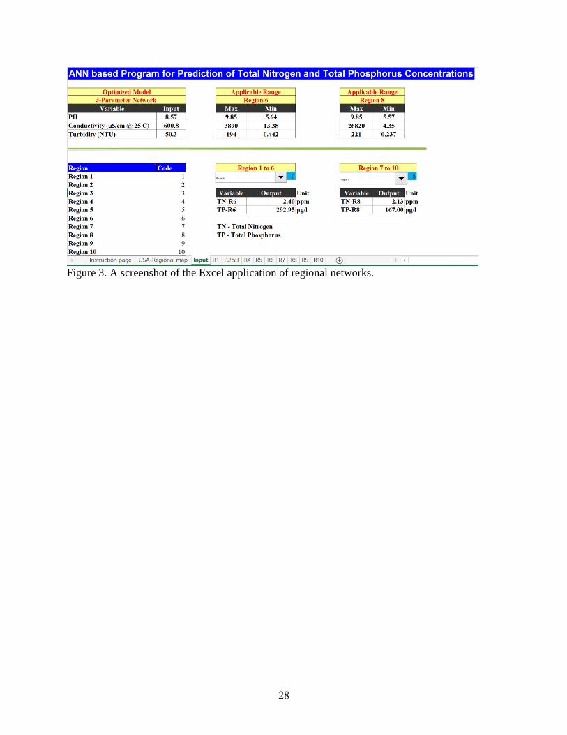
2.3.7 Excel Application

A predictive Excel application was developed for each regional network using connection

weights and threshold values of the best performing networks (Figure 3). In this Excel interface,

by entering the values of pH, conductivity, and turbidity, TN and TP can be calculated

automatically. A controlling combo box was developed to allow selection of a region of interest.

The applicable ranges for the input variables will be displayed automatically upon selecting a

region of interest. Any value of input variable that is outside of the applicable range may cause the

model to produce unreliable predictions. Further instruction on the use of the Excel application

was provided in the Excel file.

28

Figure 3. A screenshot of the Excel application of regional networks.

29

2.4 RESULTS AND DISCUSSION

2.4.1 Results from the Choice of Network Input Variables

The results of the preliminary statistical analysis of available datasets are discussed in this

section. The correlation coefficient matrix, the descriptive statistics, and the cross plots of log-

transformed training datasets for selected network variables are presented in Table 2, Table 3, and

Figure 4, respectively. Based on the specified criteria in the methodology section, pH,

conductivity, and turbidity were selected as network input variables, which were statistically

correlated to outputs for the summer season dataset with R value ≥ 0.28. The pH is an important

indicator for the presence of nutrients because it affects many chemical and biological processes

in water. The correlation analysis results between pH and output parameters were also in close

agreement. Conductivity in water indicates the presence of dissolved salts and inorganic materials,

such as chlorides, nitrates, sulfates, phosphates, sodium, magnesium, calcium, iron, and aluminum

ions. Conductivity was also significantly correlated with output parameters. Turbidity was selected

as an important indicator for output parameters because a higher nutrient load is likely associated

with a higher turbidity (USGS 2016 and U.S. EPA 2016c). These inputs are measurable with

electronic sensors in the field with direct immersion in water (U.S. EPA 2016e). The use of field

sensors is an inexpensive way of testing when compared to laboratory analysis.

30

Table 2. Correlation coefficient (R) matrix of selected network variables. Input variables Output variables

pH Conductivity Turbidity TN TP

pH 1.00

Conductivity 0.23 1.00

Turbidity 0.18 0.03 1.00

TN 0.35 0.40 0.44 1.00

TP 0.28 0.45 0.37 0.50 1.00

Table 3. Descriptive statistics of selected network variables.

pH Conductivity

(µS/cm @

25oC)

Turbidity

(NTU) TN

(mg/l) TP

(µg/l)

Maximum 10 36,000 570 26 4,900

Minimum 4.2 4.4 0.2 0.01 0

Average 7.9 480 7.1 0.76 48

Standard

Deviation

0.76 1,700 21 1.1 170

31

Figure 4. Log-distributions of training datasets. TP is total phosphorus; TN is total nitrogen (data

from U.S. EPA 2013).

2.4.2 Results from the ANN Model

The proposed feed-forward back-propagation ANN structure for the present study is

presented in Figure 5, which connects the input and output layers with one hidden layer. The nodes

in the input layer are the network input variables: pH, conductivity, and turbidity. The nodes in the

output layer are the output variables: TN and TP. The optimum number of hidden nodes and

connection weights (W) was determined during the training process.

32

Figure 5. The structure of a feed-forward back-propagation neural network for pH, conductivity,

and turbidity nodes in the input layer, and TP and TN nodes in the output layer.

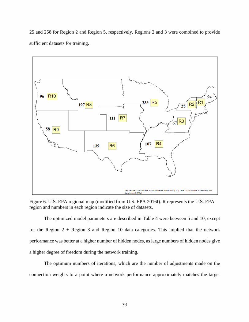
The available datasets used for training the feed-forward back-propagation neural networks

were classified into two categories. The first category consisted of the entire U.S. dataset and the

second category was comprised of datasets for the ten U.S. EPA regions (Figure 6). Using these

categories of datasets, two neural networks were fully developed and optimized: the regional and

the national datasets-based models. Overall statistical accuracy measures for all the models are

summarized in Table 3. The number of training datasets used for regional models varied between

Input

layer Hidden

layer

Output

layer

pH

Conductivity

Turbidity

TN

TP

Connection weights

33

25 and 258 for Region 2 and Region 5, respectively. Regions 2 and 3 were combined to provide

sufficient datasets for training.

Figure 6. U.S. EPA regional map (modified from U.S. EPA 2016f). R represents the U.S. EPA

region and numbers in each region indicate the size of datasets.

The optimized model parameters are described in Table 4 were between 5 and 10, except

for the Region 2 + Region 3 and Region 10 data categories. This implied that the network

performance was better at a higher number of hidden nodes, as large numbers of hidden nodes give

a higher degree of freedom during the network training.

The optimum numbers of iterations, which are the number of adjustments made on the

connection weights to a point where a network performance approximately matches the target

34

precision, were varied from 100 to 20,000. The maximum number of iterations was preset to

20,000. About 50% of the best networks for each category were obtained at 20,000 iterations.

On testing, the accuracy measures for the optimized regional networks varied from 0.00011

to 0.00140 for ASE, from 99.0 to 192.1 for MARE, and from 0.22 to 0.73 for R2. On training all,

the accuracy measures varied from 0.00025 to 0.00456 for ASE, from 75.36 to 176.48 for MARE,

and from 0. 41 to 0.94 for R2. The accuracy measures for the optimized ANN model of the national

data were ASE = 0.00094, MARE = 155.5, and R2 = 0.41 on testing, and ASE = 0.00017, MARE

= 102.14, and R2 = 0.88 on training all.

According to the ASE and MARE, the performance of nine out of the ten regional ANN

models was better than the national. The corresponding R2 values for the two categories of models

were also in close agreement with the ASE and MARE results. This is because of the relatively

higher degree of environmental homogeneity within the regional categories compared to the

combined national network. This implies that the complexity of mapping the nonlinear relationship

between water quality parameters can be simplified with the use of training data from lower level

geographical units, which have a relatively higher environmental homogeneity.

35

Table 4. Optimized model parameters for national and regional networks.

Testing Training All

No. of

Datasets

Network

(I-H-O)*

Optimum

Iteration

ASE MARE R2 ASE MARE R2

Regional Networks

R1 94 3-7-2 20000 0.00073 121.4 0.61 0.00031 139.5 0.68

R2 + R3 92 3-2-2 18100 0.00036 125.0 0.33 0.00074 141.5 0.94

R4 107 3-7-2 20000 0.00073 121.4 0.61 0.00063 130.2 0.94

R5 233 3-8-2 20000 0.00017 125.6 0.56 0.00025 117.3 0.94

R6 139 3-9-2 900 0.00144 153.1 0.73 0.00456 75.36 0.41

R7 111 3-8-2 1900 0.00030 99.0 0.72 0.00030 116.6 0.95

R8 197 3-9-2 2900 0.00021 144.8 0.60 0.00027 115.5 0.94

R9 58 3-5-2 20000 0.00059 107.5 0.62 0.00105 114.4 0.55

R10

96

3-3-2

100

0.00011

192.1

0.22

0.00366

176.48 0.58

National Network

National 1127 3-9-2 20000 0.00094 155.5 0.41 0.00017 102.14 0.88

*I-H-O represents the numbers of input nodes – the numbers of hidden nodes – the numbers of outputs, respectively.

36

According to the ASE results on testing, the Region 10, Region 5, and Region 8 networks

were the three most statistically accurate models. The Region 6 network was the lowest performing

model. One reason for the networks’ performance difference was the number of datasets. In

general, the model learns better when trained with larger datasets. The highest performing

networks were trained with the highest number of training datasets when compared to other

regions, which were 233 for Region 5 and 197 for Region 8 (186% and 157% of the average

number of regional datasets, respectively). This indicated that the ANN model’s generalizing

ability in predicting water quality was superior at a higher number of training datasets. However,

the performance of the Region 6 and Region 9 models is not consistent with the conclusion that a

higher number of training datasets results in a higher network performance. The Region 9 network,

trained with the smallest number of datasets (66), performed better than other regions trained with

a larger number of datasets. Region 6, trained with 139 datasets, was the lowest performing

network.

To understand more of what influenced the accuracy of the models, four regional

characteristics were defined and examined: total area, water area, summer temperature, and

summer precipitation (Table 5). The regions were trained with a different number of datasets. The

land and water areas were used to determine if the number of training datasets weighted with area

affect the performance of the regional networks. For this purpose, the land area and the water area

originally recorded at the state level were aggregated to a regional total, and a factor was

calculated. The total area factor was calculated as the total area of water and land per dataset. The

water area factor was similarly calculated as the total area of water per dataset (Table 6). These

two characteristics provided a general idea of the relative number of training datasets within a

given total land or water area. A higher area factor means a smaller number of training datasets.

37

The temperature (ΔT) and precipitation (ΔP) factors were used to examine if the regional climatic

difference influenced the performance of the regional networks. The climate factors were

calculated from a 30-year average of summer temperature and precipitation data. The maximum

(Max) and minimum (Min) values represented the highest and lowest selected records for states

within a given region. The ΔT and ΔP factors were calculated as simply the difference between

the maximum and minimum records of a given region.

Table 5. Regional variability characteristics of the summer season datasets. Area Temperature

(°C)

Precipitation

(mm)

Region Number of

Datasets

Total Area

(km2)

Water Area

(km2)

Max Min Max Min

R1 94 186,446 24,084 20.7 17.6 107 91

R2 + R3 92 495,287 43,576 23.4 19.2 111 99

R4 107 1,021,557 68,165 27.2 23.6 181 106

R5 233 1,005,708 170,359 23.0 19.0 105 84

R6 139 1,465,006 49,929 27.3 21.9 125 52

R7 111 739,715 6,280 24.7 22.0 111 79

R8 197 1,506,488 17,877 21.1 17.5 69 22

R9 58 1,005,581 23,577 25.1 20.6 35 7

R10 96 655,904 21,132 17.7 17.6 33 22

Sources: reprinted from Current Results (2017) and U.S. Census Bureau (2012).

38

Table 6. Regional variability factors.

Region Total Area

Factor

Water Area

Factor

ΔT Factor ΔP Factor Performan

ce Total

Area/#Dataset

s

Water

Area/#Datasets

ΔT (Max-

Min)

ΔP (Max-Min) ASEtest

R1 1,983 256 3.1 16 0.00073

R2 + R3 5,384 474 4.2 12 0.00036

R4 9,547 637 3.6 75 0.00073

R5 4,316 731 4.0 21 0.00017

R6 10,540 359 5.4 73 0.00144

R7 6,664 57 2.7 32 0.00030

R8 7,647 91 3.6 47 0.00021

R9 17,338 407 4.5 28 0.00059

R10 6,832 220 0.1 11 0.00011

The other reasons that affected the performance, other than the number of datasets, were

climatic factors related to water quality. The calculated average summer season range was

observed as lowest in Region 10, with ΔT of 0.1oC and ΔP of 11 mm, and highest in Region 6,

with ΔT of 5.4oC and ΔP of 73 mm. Region 10 was the highest performing network. In contrast,

Region 6 was the lowest performing network. This implies that a higher variability of ΔT and ΔP

made the regional data non-uniformly noisy to the extent that its performance could not be

improved by more datasets.

A further comparison of the regional networks’ performance was made using a correlation

analysis between ASE on testing and the four factors (Table 7). According to this correlation

analysis, the performance of the regional models was strongly correlated to temperature and

precipitation, with R of 0.60 and 0.65, respectively. The average of the four normalized factors

was further used to produce an aggregated factor. The correlation between the aggregated factor

and performance was 0.62. The lowest performing networks, as was seen in Region 6, were

associated with a higher regional climate difference. A higher climatic variability due to a higher

39

ΔT or ΔP likely means a higher ASE value, or a lower performance of the regional network. These

results revealed the regional data dependence on climatic factors. The use of a dataset within a

homogenous climactic region is likely to improve the learning ability of ANN models.

Table 7. Correlation coefficient matrix between the ASE on testing and the regional variability

factors.

Total Area

Factor

Water Area

Factor

ΔT

Factor

ΔP

Factor

Aggregated

Factor

ASEtest 0.31 0.13 0.60 0.65 0.62

2.4.3. Results from the Regression Model

A linear regression model was developed using the training datasets used for ANN model

development. Its input and output variables were the same as those used in the ANN models. Using

a linear regression approach, Equations 12 and 13 were developed.

TN = -3.75 + 0.553pH + 0.000272Conductivity + 0.0240Turbidity (Equation 3)

TP = -349.82 + 48.617pH + 0.04640Conductivity + 3.0036Turbidity (Equation 4)

The R2 statistical measure of the linear regression models was 0. 39 for TN and 0.35 for

TP.

A comparison of the linear regression and ANN models was performed using the Region

7 and Region 1 networks as examples. With the same validation datasets, a prediction was made

for TN using the developed ANN and linear regression models. The plots for predicted and

observed responses are shown in Figure 7. The R2 results for predictions from the linear regression

model were 0.41 and 0.79 for Region 1 and Region 7, respectively; and from ANN model were

0.61 and 0.96 for Region 1 and Region 7, respectively. The R2 results for predictions from the

linear regression model were 0.41 and 0.79 for Region 1 and Region 7, respectively; and from the

40

ANN model were 0.61 and 0.96 for Region 1 and Region 7, respectively. The R2 for predictions

obtained from the ANN model in both regions was higher than that obtained from the linear

regression model. The performance of the regional networks was further validated using a database

from the 2012 survey of the U.S. EPA National Lake Assessment. The R2 results for prediction of

TN and TP using the Region 7 network were 0.75 and 0.60, respectively (Figure 8). These results

indicate that the ANN models consistently outperformed the linear regression model. This implies

that the non-linear behavior of water quality parameters was better handled by the ANN model.

41

Figure 7. Prediction accuracy for linear regression and ANN models using the 2007 datasets.

Figure 8. Prediction accuracy of Regional ANN model using the 2012 U.S. EPA National Lake

Assessment data.

2.4.4 Results from the Sensitivity Analysis

The sensitivity analysis was performed using the Region 1 network as an example. The

results of the sensitivity analysis are presented in Figure 9 and Table 8. Figure 9 demonstrated that

the output parameters were impacted by the change in the values of each of the values of the input

variable. Table 7 showed sensitivity index results, where a 10% change of each input resulted in a

maximum of 80.00% and a minimum of 1.73% change in TN, and a maximum of 47.89% and a

minimum of 0.27% change in TP. TN was most to least sensitive to pH, turbidity, and conductivity,

respectively. TP was most to least sensitive to pH, conductivity, and turbidity, respectively.

Overall, pH had the most substantial influence on the prediction of both TN and TP. These results

imply that a small change in the value of the selected input variables can considerably influence

the output values.

42

Figure 9. Sensitivity results of outputs TN and TP to inputs pH, conductivity, and turbidity using

Region 1 as an example.

Table 8. Sensitivity index values of network outputs to input variables.

pH Conductivity Turbidity

Changes in

input

variables

+10.00%

-10.00%

+10.00%

-10.00%

+10.00%

-10.00%

Associated

responses of

outputs

TN +80.00% -30.00% +2.45% -1.73% +3.52% -3.50%

TP

+47.89%

-23.90%

+5.01%

-3.53%

+0.27%

-0.29%

2.5 CONCLUSIONS

In this study, the ability of the ANN model to predict TN and TP concentrations using

easily measurable water quality variables, namely pH, conductivity, and turbidity, was explored

and justified in the case of U.S. lakes during summer months. This study developed two ANN

models that were trained by regional and national datasets. The performance of the ANN models’

prediction accuracy was assessed using the average of squared error, mean absolute relative error,

and coefficient of determination.

The ANN models were found suitable to estimate TN and TP concentrations in both the

national and the regional datasets when compared to counterpart linear regression models. This

observation indicates that the ANN-based models are superior to linear regression models in water

quality modeling tasks. The statistical accuracy of the ANN models was improved when the

network was trained using regional datasets rather than the national dataset. This implies that their

generalizing capabilities are better in geographically and climatologically homogenous regions.

Further, a better network performance was observed for models developed with a relatively higher

number of datasets and located in relatively homogenous temperature and precipitation zones. The

regional ANN models that consider all three water quality variables can be suggested as a tool for

estimation of TN and TP summer concentrations in U.S. lakes. A sensitivity analysis showed that

pH, turbidity, and conductivity were the most to the least important indicators of nutrient

concentrations. The proposed ANN model can be a useful alternative to laboratory analysis of TP

and TN for lakes in the summer season.

44

This study suggests the following procedures to achieve a desired level of accuracy: (1)

using large training datasets, and (2) using datasets with relatively homogeneous temperature and

precipitation. Large datasets are rarely available for water quality variables. The use of training

datasets that represent a certain class of climatic zones can compensate for small datasets. It is

further suggested to investigate the impact of other environmental factors, such as land use,

geology, soil, and other climatic factors to understand ANN modeling of water quality parameters

discussed in this study.

45

LIST OF REFERENCES

46

Anmala, J., Meier, O. W., Meier, A. J., and Grubbs, S. (2015). “GIS and Artificial Neural

Network–Based Water Quality Model for a Stream Network in the Upper Green River Basin,

Kentucky, USA.” Journal of Environmental Engineering, 141(5), 4014082.

APHA (American Public Health Association), (1995). “Standard methods for the examination of

water and wastewater.” 16th ed. Washington, DC, New York.

Boomer, K. M. B., Weller, D. E., Jordan, T. E., Linker, L., Liu, Z. J., Reilly, J., Shenk, G., and

Voinov, A. A. (2013). “Using Multiple Watershed Models to Predict Water, Nitrogen, and

Phosphorus Discharges to the Patuxent Estuary.” Journal of the American Water Resources

Association, 49(1), 15–39.

Current Results (2017). “Weather and science facts.”

https://www.currentresults.com/Weather/US/weather-averages-index.php. (Jan. 27, 2017).

Gazzaz, N. M., Yusoff, M. K., Aris, A. Z., Juahir, H., and Ramli, M. F. (2012). “Artificial neural

network modeling of the water quality index for Kinta River (Malaysia) using water quality

variables as predictors.” Marine Pollution Bulletin, 64(11), 2409–2420.

Hatvani, I. G., Kovács, J., Márkus, L., Clement, A., Hoffmann, R., and Korponai, J. (2015).

“Assessing the relationship of background factors governing the water quality of an

agricultural watershed with changes in catchment property (W-Hungary).” Journal of

Hydrology, 521, 460–469.

Haykin S. (1999). “Neural Networks: A Comprehensive Foundation,” 2nd Edition, Prentice-Hall

NJ, USA.

Itani, O. M., and Najjar, Y. (2000). “Three-dimensional modeling of spatial soil properties via

artificial neural networks.” Geotechnical Aspects of Pavements 2000, (1709), 50–59.

Jones, K. B., Neale, A. C., Nash, M. S., Van Remortel, R. D., Wickham, J. D., Riitters, K. H., and

O'Neill, R. V. (2001). "Predicting nutrient and sediment loadings to streams from landscape

metrics: A multiple watershed study from the United States Mid-Atlantic Region." Landscape

Ecol., 16(4), 301-312.

Jones, K. B., Neale, A. C., Nash, M. S., Van Remortel, R. D., Wickham, J. D., Riitters, K. H., and

O’neill, R. V. (2001). “Predicting nutrient and sediment loadings to streams from landscape

metrics: A multiple watershed study from the United States Mid-Atlantic Region.” Landscape

Ecology, 16(4), 301–312.

Keskin, T. E., Dugenci, M., and Kaçaroglu, F. (2015). “Prediction of water pollution sources using

artificial neural networks in the study areas of Sivas, Karabuk and Bartın (Turkey).”

Environmental Earth Sciences, 73(9), 5333–5347.

Khalil, B., Ouarda, T. B. M. J., and St-Hilaire, A. (2011). "Estimation of water quality

characteristics at ungauged sites using artificial neural networks and canonical correlation

47

analysis." J. of Hydrology, 405(3-4; 3-4), 277-287.

Kosten, S., Vera L. M. Huszar, Mazzeo, N., Scheffer, M., Leonel Da S. L. Sternberg, and Jeppesen,

E. (2009). "Lake and watershed characteristics rather than climate influence nutrient

limitation in shallow lakes." Ecol.Appl., 19(7), 1791-1804.

Maier, H. R., Jain, A., Dandy, G. C., and Sudheer, K. P. (2010). "Review: Methods used for the

development of neural networks for the prediction of water resource variables in river

systems: Current status and future directions." Env. Modelling and Software, 25 891-909.

Milstead, W. B., Hollister, J. W., Moore, R. B., and Walker, H. A. (2013). "Estimating summer

nutrient concentrations in Northeastern lakes from SPARROW load predictions and modeled

lake depth and volume: e81457." PLoS One, 8(11).

Najjar, Y., M. (1999). “Quick Manual for TR-SEQ1”. Department of Civil Engineering, Kansas

State University, Manhattan, Kansas, USA.

Najjar, Y. M., Basheer, I. A., and Naouss, W. A. (1996). “On the Identification of Compaction

Characteristics by Neuronets.” Computers and Geotechnics, 18(3), 167–187.

Najjar, Y. M., and Huang, C. (2007). “Simulating the stress-strain behavior of Georgia kaolin via

recurrent neuronet approach.” Computers and Geotechnics, 34(5), 346–361.

Olawoyin, R., Nieto, A., Grayson, R. L., Hardisty, F., and Oyewole, S. (2013). "Application of

artificial neural network (ANN) self-organizing map (SOM) for the categorization of water,

soil and sediment quality in petrochemical regions." Expert Systems with Applications, 40(9),

3,634-3,648.

Pannell, D.J. (1997). “Sensitivity analysis of normative economic models: Theoretical framework

and practical strategies.” Agricultural Economics 16: 139-152.

Portielje, R., and Van, d. M. (1999). "Relationships between eutrophication variables: From

nutrient loading to transparency." Hydrobiologia, (408-409), 375-387.

Rode, M., Arhonditsis, G., Balin, D., Kebede, T., Krysanova, V., Griensven, A., and Zee, v. d.,

S.E.A.T.M. (2010). "New challenges in integrated water quality modelling." Hydrol.Process.,

24(24), 3447-3461.

Rumelhart, D. and McClelland J. (1986). "Parallel distributed processing." MIT Press, Cambridge,

Mass.

Sibanda, W., and Pretorius, P. (2012). “Artificial neural networks: A review of applications of

neural networks in the modeling of HIV epidemic.” Volume 44-No16.

Stow, C. A., Roessler, C., Reckhow, K. H., Borsuk, M. E., and Bowen, J. D. (2003). "Comparison

of estuarine water quality models for total maximum daily load development in Neuse River

48

estuary." J.Water Resour.Plann.Manage., 129(4), 307-314.

U.S. Census Bureau (2012). “The land, water, and total area measurements of 50 states.”

https://www.census.gov/geo/reference/state-area.html. (Jan. 27, 2017).

U.S. Environmental Protection Agency (2013). “National Aquatic Resource Surveys A national

lake assessment report.” https://www.epa.gov/national-aquatic-resource-surveys/nla (Sept.

15, 2016).

U.S. Environmental Protection Agency. (2018a). CFR (Code of Federal Regulations). “Guidelines

establishing test procedures for the analysis of pollutants, part 136.” <

https://www.ecfr.gov/cgi-bin/text-

idx?SID=a6bb8a02b6d783f9356758b5ff0ed106&mc=true&node=pt40.25.136&rgn=div5>(

Apr. 12, 2018)

U.S. Environmental Protection Agency (2016b). “Nutrient pollution problem.”

https://www.epa.gov/nutrientpollution/problem. (Sept. 15, 2016).

U.S. Environmental Protection Agency (2016c). “CADDIS Volume 2: sources, stressors &

responses.” https://www3.epa.gov/caddis/ssr_ph_int.html. (Sept. 15, 2016).

United States Geological Survey (2016). “Water Properties and measurements.”

https://water.usgs.gov/edu/waterproperties.html. (sep. 15, 2016).

Wu, M., Wang, Y.S., and Gu, J. (2015). "Assessment for water quality by artificial neural network

in Daya Bay, South China Sea." Ecotoxicology, 24(7-8), 1632-1642.

Wu, W., Dandy, G. C., and Maier, H. R. (2014). "Review: Protocol for developing ANN models

and its application to the assessment of the quality of the ANN model development process

in drinking water quality modelling." Env. Modelling and Software, 54 108-127.

Varol, M. (2013). “Temporal and spatial dynamics of nitrogen and phosphorous in surface water

and sediments of a transboundary river located in the semi-arid region of Turkey.” Catena,

100(0), 1-9.

Zelenakova, M., Carnogurska, M., Slezingr, M., Slys, D., and Purcz, P. (2013). "A model based

on dimensional analysis for prediction of nitrogen and phosphorus concentrations at the river

station Izkovce, Slovakia." Hydrology and Earth System Sciences, 17(1), 201-209.

49

APPENDIX

50

A description of water quality data used in this research is provided in this appendix.

1. Sampled lakes

The U.S. EPA National Lake Assessment (NLA) surveys U.S. lakes every 5 years to assess

their water quality condition. This study used the 2007 survey for developing regional networks.

The 2012 survey (which was published in December 2017) was used to validate the regional

models. About 1,038 sampled lakes were considered as reference lakes to represent approximately

50,000 freshwater natural or man-made lakes, ponds, and reservoirs. The survey excluded Great

Lakes, commercial treatment and disposal ponds, brackish lakes, or ephemeral lakes.

2. Sampled Water Quality Indicators

The purpose of the U.S. EPA NLA survey is to assess the biological, chemical, physical

and recreational condition of lakes. Approximately 52 indicators were used to characterize the

conditions of lakes. Examples of measured indicators are shown in Table 9.

Table 9. Examples of measured indicators under the U.S. EPA NLA program.

Biological Chemical Physical Recreational

Benthic

macroinvertebrates

Acidification Lakeshore

habitat/riparian

vegetative cover

Algal toxins

(Microcystin)

Chlorophyll a Atrazine Human

disturbance

Cyanobacteria

Fish assemblage Conductivity Physical habitat

complexity

Enterococci

Fish tissue

contaminants

Dissolved

oxygen

Shallow water

habitat/in-stream

fish habitat

Fish tissue

contaminants

Macrophytes Nitrogen Streambed

sediments

Algal toxins

(Microcystin)

Phytoplankton Phosphorus Water clarity Cyanobacteria

Sediment diatoms Salinity Lakeshore

habitat/riparian

vegetative cover

Wetland vegetation

(introduced species)

Sediment

enzymes

Human

disturbance

51

3. Data Used for Training the Regional Networks

The data used for model development for network variables are summarized in Table 10.

Table 10. Measured data for selected network variables. Site ID EPA

Region

Sampling

Date

pH Conductivity

(µS/cm @ 25oC)

Turbidity

(NTU)

TN

(mg/l)

TP

(µg/l)

NLA06608-0001 Region_1 7/31/2007 7.63 96.28 0.474 0.151 6

NLA06608-0005 Region_1 8/22/2007 7.7 56.1 0.591 0.048 2

NLA06608-0005 Region_1 8/22/2007 7.7 54.96 0.609 0.068 3

NLA06608-0024 Region_1 8/14/2007 7.33 142.5 3.83 0.943 29

NLA06608-0025 Region_1 7/18/2007 7.73 89.09 1.42 0.097 4

NLA06608-0025 Region_1 6/18/2007 7.63 84.96 1.56 0.195 10

NLA06608-0025 Region_1 7/18/2007 7.75 89.23 1.12 0.089 5

NLA06608-0037 Region_1 7/13/2007 7.15 98.02 2.59 0.239 14

NLA06608-0038 Region_1 8/27/2007 7.48 62.84 0.654 0.113 3

NLA06608-0071 Region_1 9/6/2007 8.72 245.2 12.9 2.369 399

NLA06608-0071 Region_1 9/8/2007 8.72 248 10.7 2.268 390

NLA06608-0077 Region_1 9/8/2007 8.54 308.4 17.4 1.461 116

NLA06608-0083 Region_1 6/13/2007 8.86 4281 1.37 3.925 50

NLA06608-0089 Region_1 6/17/2007 7.44 62.86 3.14 0.333 35

NLA06608-0091 Region_1 7/10/2007 9.03 325.9 35.5 2.021 170

NLA06608-0110 Region_1 7/31/2007 8.56 260.1 1.17 0.491 12

NLA06608-0128 Region_1 6/21/2007 8.42 517.7 21.9 1.356 76

NLA06608-0167 Region_1 7/23/2007 9.75 1523 193 15.625 1184

NLA06608-0175 Region_1 8/30/2007 8.47 365.2 5.18 0.698 55

NLA06608-0208 Region_1 9/6/2007 6.72 124.9 20.7 1.687 162

NLA06608-0209 Region_1 7/19/2007 8.09 107.9 0.597 0.205 4

NLA06608-0223 Region_1 6/27/2007 7.68 81.15 7.01 0.569 45

NLA06608-0237 Region_1 7/17/2007 8.33 685.3 1.23 0.588 25

NLA06608-0239 Region_1 7/24/2007 8.1 194.4 3.98 0.383 36

52

NLA06608-0240 Region_1 7/25/2007 8.57 552.7 1.52 0.396 14

NLA06608-0247 Region_1 7/17/2007 8.55 1652 7.24 1.625 202

NLA06608-0281 Region_1 6/20/2007 7.87 131 8.1 0.639 44

NLA06608-0294 Region_1 6/26/2007 8.4 310.7 0.85 0.343 1

NLA06608-0303 Region_1 8/7/2007 8.46 584 8.94 1.523 79

NLA06608-0328 Region_1 9/15/2007 7.88 179.1 9.31 1.12 75

NLA06608-0343 Region_1 8/21/2007 8.78 1554 10.4 2.606 117

NLA06608-0377 Region_1 7/12/2007 8.53 153.6 5.51 0.85 46

NLA06608-0421 Region_1 6/28/2007 7.78 451.6 1.08 0.537 9

NLA06608-0426 Region_1 9/17/2007 8.31 206.2 1.48 0.574 5

NLA06608-0440 Region_1 8/8/2007 8.16 201.9 103 0.853 182

NLA06608-0442 Region_1 8/14/2007 8.84 2360 8.19 6.559 385

NLA06608-0456 Region_1 8/9/2007 8.44 450.7 3.66 0.681 29

NLA06608-0484 Region_1 7/12/2007 7.7 79.49 19.4 1.519 190

NLA06608-0529 Region_1 9/4/2007 8.83 276.1 7.01 0.508 42

NLA06608-0540 Region_1 8/27/2007 8.29 1255 31.7 2.25 235

NLA06608-0550 Region_1 8/1/2007 6.85 27.88 0.454 0.234 1

NLA06608-0562 Region_1 8/21/2007 6.87 113.2 1.24 0.28 4

NLA06608-0562 Region_1 8/21/2007 6.88 112.9 1.27 0.25 5

NLA06608-0580 Region_1 8/7/2007 8.36 688 0.775 0.183 10

NLA06608-0594 Region_1 8/9/2007 7.19 58.43 6.31 0.821 41

NLA06608-0606 Region_1 8/8/2007 7.33 151 5.18 0.708 15

NLA06608-0616 Region_1 7/25/2007 8.3 1211 1.15 0.483 14

NLA06608-0659 Region_1 6/26/2007 8.44 888.5 8.74 1.593 432

NLA06608-0661 Region_1 8/8/2007 8.31 204 7.39 0.601 22

NLA06608-0662 Region_1 8/7/2007 7.46 68.4 1.64 0.256 12

NLA06608-0783 Region_1 8/14/2007 8.57 600.8 50.3 1.896 819

NLA06608-0785 Region_1 9/12/2007 8.42 406.2 2.15 2.621 15

NLA06608-0794 Region_1 6/9/2007 6.59 20.49 0.416 0.091 3

NLA06608-0807 Region_1 7/11/2007 8.76 1893 14.2 1.505 511

NLA06608-0825 Region_1 9/6/2007 8.46 793.6 21 1.001 88

53

NLA06608-0851 Region_1 6/5/2007 8.29 4321 5.17 1.104 44

NLA06608-0863 Region_1 7/2/2007 7.75 225.7 4.88 0.446 36

NLA06608-0865 Region_1 9/12/2007 8.34 187.9 12.6 1.489 100

NLA06608-0875 Region_1 9/14/2007 8.07 294.2 2.38 0.72 16

NLA06608-0972 Region_1 7/9/2007 7.54 311.8 140 0.938 619

NLA06608-0979 Region_1 5/30/2007 7.46 392.1 1.07 0.952 68

NLA06608-1014 Region_1 9/13/2007 8.31 683.3 1.33 0.568 15

NLA06608-1060 Region_1 8/14/2007 8.94 113.9 19.5 2.372 243

NLA06608-1086 Region_1 8/27/2007 9 7200 13.8 3.95 92

NLA06608-1261 Region_1 6/25/2007 8.9 821.2 3.01 1.014 32

NLA06608-1360 Region_1 8/19/2007 8.22 289.7 11.8 0.734 60

NLA06608-1387 Region_1 7/20/2007 8.43 437.1 5.02 0.994 25

NLA06608-1641 Region_1 6/19/2007 8.14 179.3 67.6 0.845 185

NLA06608-1742 Region_1 7/18/2007 6.07 14.87 0.596 0.244 7

NLA06608-1811 Region_1 6/25/2007 8.97 2137 3.39 1.558 27

NLA06608-1874 Region_1 8/14/2007 8.49 466.5 3.68 0.374 26

NLA06608-1893 Region_1 7/12/2007 8.53 391 76.1 0.581 302

NLA06608-1998 Region_1 8/6/2007 6.82 23.05 1.51 0.43 13

NLA06608-2463 Region_1 7/19/2007 8.33 595.2 1.52 0.183 6

NLA06608-2477 Region_1 6/26/2007 8.93 1399 2.52 1.238 32

NLA06608-2481 Region_1 8/1/2007 7.7 216.1 8.75 0.421 36

NLA06608-2523 Region_1 7/31/2007 8.58 506.3 6.61 1.259 56

NLA06608-2566 Region_1 7/12/2007 7.79 261 1.88 0.376 9

NLA06608-2714 Region_1 8/11/2007 7.25 923 1.49 0.216 8

NLA06608-2715 Region_1 8/17/2007 8.48 572.7 11.7 0.369 36

NLA06608-2726 Region_1 9/12/2007 8.24 152.3 0.61 0.191 5

NLA06608-2753 Region_1 8/30/2007 9.15 1514 1.88 1.496 16

NLA06608-2759 Region_1 8/30/2007 7.51 382.4 1.93 0.206 9

NLA06608-2776 Region_1 10/16/2007 7.72 208.6 5.82 1.144 36

NLA06608-2779 Region_1 7/18/2007 8.45 476.3 1.66 0.713 21

NLA06608-2797 Region_1 6/28/2007 8.69 646.2 3.27 0.664 24

54

NLA06608-2800 Region_1 9/25/2007 8.17 380.3 2.3 0.235 11

NLA06608-2801 Region_1 8/1/2007 8.45 808.5 22.5 0.339 36

NLA06608-2807 Region_1 8/13/2007 8.54 1380 3.39 0.66 32

NLA06608-2823 Region_1 9/5/2007 6.96 52.1 3.5 0.751 31

NLA06608-2824 Region_1 8/13/2007 8.78 144.1 6.81 0.794 208

NLA06608-2831 Region_1 8/1/2007 8.29 205.1 13.2 0.738 107

NLA06608-2891 Region_1 7/16/2007 8.61 439.5 1.53 0.79 8

NLA06608-2916 Region_1 39288 8.33 186.5 1.33 0.324 15

NLA06608-2924 Region_1 8/1/2007 8.31 2795 3.5 0.693 13

NLA06608-2954 Region_1 7/26/2007 8.94 124.3 214 7.684 876

NLA06608-2955 Region_1 6/28/2007 8.65 207.9 5.65 0.513 58

NLA06608-3484 Region_1 8/20/2007 9.25 847.7 78.1 4.319 180

NLA06608-3608 Region_1 8/16/2007 8.85 544.1 15.3 1.821 191

NLA06608-3616 Region_1 7/30/2007 8.42 772.1 4.78 0.455 15

NLA06608-3644 Region_1 8/15/2007 8.75 922.3 11 2.063 58

NLA06608-3656 Region_1 8/22/2007 7.38 425.6 23.3 5.813 471

NLA06608-3660 Region_1 8/23/2007 8.06 135.2 312 2.263 1329

NLA06608-3698 Region_1 7/19/2007 6.92 92.81 1.09 0.3 6

NLA06608-3846 Region_1 7/12/2007 6.83 45.2 0.387 0.11 3

NLA06608-3890 Region_1 7/11/2007 6.31 51.33 0.665 0.098 1

NLA06608-0010 Region_2 8/18/2007 8.59 648.6 1.42 0.485 10

NLA06608-0010 Region_2 39274 8.74 650.1 3.05 0.473 10

NLA06608-0015 Region_2 8/29/2007 8.41 706.4 17.7 0.423 98

NLA06608-0015 Region_2 7/10/2007 8.36 743.6 32.7 0.47 109

NLA06608-0038 Region_2 8/27/2007 7.48 61.5 0.447 0.101 3

NLA06608-0038 Region_2 7/12/2007 7.62 59.7 0.549 0.158 4

NLA06608-0057 Region_2 39322 7.78 151.8 12.3 1.219 188

NLA06608-0057 Region_2 39296 7.76 152.3 12.5 0.939 212

NLA06608-0168 Region_2 6/13/2007 8.21 211.5 16.9 0.866 61

NLA06608-0225 Region_2 8/24/2007 8.22 369.4 1.61 0.506 46

NLA06608-0228 Region_2 8/6/2007 7.9 851 9.19 0.71 96

55

NLA06608-0295 Region_2 6/26/2007 8.65 1240 10.5 2.026 242

NLA06608-0407 Region_2 7/23/2007 8.96 1403 1.8 2.872 762

NLA06608-0614 Region_2 6/27/2007 8.03 219.4 0.825 0.259 8

NLA06608-0622 Region_2 39261 8.59 379.6 3.66 0.508 16

NLA06608-0637 Region_2 8/6/2007 8.63 249 9.23 0.454 21

NLA06608-0862 Region_2 8/8/2007 7.26 60.21 1.16 0.654 11

NLA06608-0899 Region_2 39273 8.85 6864 20.4 4.472 495

NLA06608-0913 Region_2 9/6/2007 7.99 98.49 3.4 0.697 10

NLA06608-0944 Region_2 39279 7.92 404.2 296 1.419 523

NLA06608-1035 Region_2 8/14/2007 8.71 411.4 34.3 4.348 160

NLA06608-1124 Region_2 39342 9.08 423.7 2.16 0.433 9

NLA06608-1172 Region_2 6/27/2007 8.19 181.5 1.48 0.241 4

NLA06608-1210 Region_2 8/15/2007 9.12 12600 2.8 4.184 75

NLA06608-2740 Region_2 39372 8.5 205.8 9.8 0.359 121

NLA06608-0020 Region_3 7/2/2007 8.33 220.1 3.98 0.444 20

NLA06608-0020 Region_3 6/11/2007 8.43 214.1 4.55 0.605 30

NLA06608-0029 Region_3 7/2/2007 7.37 141.7 25.1 2.106 247

NLA06608-0029 Region_3 9/11/2007 8.56 146.7 16.4 2.146 162

NLA06608-0036 Region_3 7/12/2007 8.23 133.5 1.57 0.178 8

NLA06608-0036 Region_3 7/16/2007 8.64 130.1 1.33 0.348 9

NLA06608-0044 Region_3 7/18/2007 8.67 274.1 121 4.108 601

NLA06608-0045 Region_3 8/2/2007 7.33 116.9 9.17 0.43 60

NLA06608-0085 Region_3 8/20/2007 8.83 236.9 72.9 1.518 395

NLA06608-0089 Region_3 7/17/2007 8.17 68.27 4.61 0.401 31

NLA06608-0090 Region_3 7/25/2007 6.14 38.67 0.858 0.449 16

NLA06608-0120 Region_3 9/26/2007 7.78 914.7 17.1 1.256 180

NLA06608-0124 Region_3 7/19/2007 9.49 7382 15.9 0.34 213

NLA06608-0126 Region_3 6/21/2007 8.96 1482 46.8 5.728 502

NLA06608-0149 Region_3 7/18/2007 7.83 118 1.12 0.22 12

NLA06608-0203 Region_3 8/2/2007 7.42 55.09 1.15 0.239 1

NLA06608-0222 Region_3 6/27/2007 8.72 1705 3.54 2.008 114

56

NLA06608-0235 Region_3 7/16/2007 8.51 443.2 3.22 0.626 8

NLA06608-0257 Region_3 7/18/2007 8.65 217.6 0.784 0.079 1

NLA06608-0271 Region_3 6/27/2007 8.36 418.1 35.7 0.857 99

NLA06608-0286 Region_3 8/8/2007 6.53 22.17 0.762 0.413 5

NLA06608-0291 Region_3 7/11/2007 8.64 496.1 1.68 0.553 13

NLA06608-0341 Region_3 9/18/2007 8.34 358.7 1.51 0.333 23

NLA06608-0363 Region_3 7/21/2007 8.52 475 1.93 0.567 18

NLA06608-0367 Region_3 8/23/2007 8.63 339.3 8.2 2.157 54

NLA06608-0388 Region_3 8/16/2007 7.14 40.34 1.37 0.085 3

NLA06608-0399 Region_3 7/16/2007 8.43 460.7 1.08 0.586 13

NLA06608-0408 Region_3 6/20/2007 8.19 346.4 6.58 0.27 15

NLA06608-0414 Region_3 7/31/2007 7.41 58.79 3.06 1.296 40

NLA06608-0453 Region_3 7/31/2007 6 93.31 2.36 1.056 48

NLA06608-0537 Region_3 6/6/2007 7.17 150.2 2.81 0.256 11

NLA06608-0560 Region_3 9/12/2007 8.49 3256 8.15 0.532 27

NLA06608-0587 Region_3 7/9/2007 8.3 257.7 4.99 1.153 29

NLA06608-0610 Region_3 8/2/2007 7.65 300.7 2.52 0.549 11

NLA06608-0625 Region_3 9/19/2007 6.82 21.56 0.53 0.055 1

NLA06608-0651 Region_3 7/17/2007 8.7 222.4 2.08 0.29 12

NLA06608-0738 Region_3 8/16/2007 6.27 30.48 0.539 0.223 3

NLA06608-0830 Region_3 8/30/2007 8.61 5769 233 15.563 1617

NLA06608-0860 Region_3 8/21/2007 8.1 421.7 21.7 1.71 232

NLA06608-0871 Region_3 7/12/2007 8.6 848.5 68.5 5.378 407

NLA06608-0990 Region_3 7/30/2007 8.7 200.8 6.59 0.96 40

NLA06608-1056 Region_3 9/27/2007 7.58 93.75 4.02 0.464 22

NLA06608-1189 Region_3 9/21/2007 6.71 89.54 0.74 0.281 9

NLA06608-1191 Region_3 8/6/2007 7.78 445.7 8.81 0.984 152

NLA06608-1240 Region_3 7/18/2007 7.92 244.9 2.56 0.771 141

NLA06608-1241 Region_3 6/23/2007 7.66 82.43 5.75 0.526 34

NLA06608-1256 Region_3 7/17/2007 8.46 406.2 3.47 0.346 20

NLA06608-1266 Region_3 7/12/2007 8.02 140.7 574 2.228 933

57

NLA06608-1303 Region_3 8/8/2007 8.81 425.4 5.86 2.338 817

NLA06608-1347 Region_3 6/28/2007 8.09 121.2 1.72 0.551 12

NLA06608-1358 Region_3 9/18/2007 7.65 80.57 1.02 0.359 7

NLA06608-1365 Region_3 8/21/2007 8.48 426.2 4.01 0.257 13

NLA06608-1420 Region_3 9/18/2007 7.9 121.2 79.1 1.154 112

NLA06608-1508 Region_3 8/20/2007 8.22 561.8 13 1.68 313

NLA06608-1537 Region_3 7/15/2007 8.07 80.23 0.67 0.138 8

NLA06608-1572 Region_3 8/20/2007 7.92 554.9 7.6 0.42 26

NLA06608-1781 Region_3 10/2/2007 7.81 198.9 12.5 0.789 58

NLA06608-1856 Region_3 7/24/2007 10.09 706.9 38.9 3.159 1129

NLA06608-1871 Region_3 7/19/2007 7.46 39.65 3.23 0.139 5

NLA06608-4686 Region_3 9/12/2007 6.85 79.17 36.2 0.446 84

NLA06608-4698 Region_3 9/16/2007 7.81 297.2 7.44 1.333 142

NLA06608-4828 Region_3 9/4/2007 8.32 366.8 4.87 0.421 24

NLA06608-4929 Region_3 7/17/2007 8.15 289.9 3.67 0.954 121

NLA06608-4949 Region_3 8/29/2007 7.84 229.2 9.66 0.623 82

NLA06608-9999 Region_3 7/31/2007 7.17 28.99 0.516 0.149 1

NLA06608-ACAD_LAKES_0435 Region_3 8/1/2007 6.67 27.54 0.555 0.151 10

NLA06608-ALPS-1218 Region_3 8/3/2007 4.57 18.23 2.47 0.414 14

NLA06608-ALSC:020149 Region_3 9/11/2007 7.02 28.61 0.752 0.191 5

NLA06608-ELS:1C2-032 Region_3 7/12/2007 6.78 29.79 4.86 0.264 11

NLA06608-ELS:1C3-003 Region_3 8/15/2007 6.81 18.07 0.64 0.256 9

NLA06608-ELS:1D1-035 Region_3 7/25/2007 7.2 54.16 6.3 0.444 23

NLA06608-ELS:1D2-087 Region_3 7/27/2007 6.54 57.59 3.92 0.532 35

NLA06608-ELS:1E1-052 Region_3 8/7/2007 6.85 21 0.458 0.13 10

NLA06608-ELS:1E1-096 Region_3 8/9/2007 6.67 20.48 1.46 0.236 9

NLA06608-0002 Region_4 7/23/2007 5.93 43.18 3.87 0.469 22

NLA06608-0002 Region_4 39301 6.05 44.8 3.55 0.695 36

NLA06608-0019 Region_4 39277 9.15 3952 29.7 5.603 1414

NLA06608-0019 Region_4 39343 9.05 3950 33.8 6.578 1376

NLA06608-0041 Region_4 7/11/2007 7.46 85.47 0.936 0.37 1

58

NLA06608-0041 Region_4 39343 7.37 82.91 0.601 0.476 1

NLA06608-0048 Region_4 8/2/2007 8.46 223.9 16.7 0.773 111

NLA06608-0048 Region_4 9/18/2007 8.33 245.6 18.2 0.943 82

NLA06608-0066 Region_4 39273 7.37 126 2.71 0.626 6

NLA06608-0066 Region_4 39254 7.36 126.6 2.54 0.574 6

NLA06608-0091 Region_4 8/13/2007 9.31 329.2 40.9 2.411 164

NLA06608-0126 Region_4 39295 9.15 1494 50.7 7.019 609

NLA06608-0129 Region_4 7/21/2007 8.36 248.8 3.09 0.139 4

NLA06608-0129 Region_4 7/21/2007 8.4 244 0.264 0.108 5

NLA06608-0130 Region_4 8/13/2007 8.41 159.2 1.97 2.234 36

NLA06608-0144 Region_4 9/13/2007 7.83 433.3 20.3 0.751 68

NLA06608-0152 Region_4 7/17/2007 8.55 473.6 4.44 0.521 21

NLA06608-0153 Region_4 8/30/2007 7.61 95.33 4.09 0.656 34

NLA06608-0174 Region_4 8/28/2007 8.88 663.2 1.68 0.786 12

NLA06608-0179 Region_4 8/29/2007 8.56 16930 18.1 7.522 272

NLA06608-0181 Region_4 9/20/2007 8.54 303.3 0.58 0.514 6

NLA06608-0196 Region_4 39296 8.67 170.3 11.4 1.25 94

NLA06608-0198 Region_4 7/24/2007 6.85 106.3 2.06 0.353 25

NLA06608-0209 Region_4 39254 8.07 106.8 0.7 0.201 6

NLA06608-0219 Region_4 39301 8.59 383.9 22.1 1.826 36

NLA06608-0221 Region_4 39302 7.98 190.7 11.2 0.594 38

NLA06608-0223 Region_4 8/29/2007 7.64 89.63 8.65 0.713 43

NLA06608-0223 Region_4 8/29/2007 7.58 89.51 8.62 0.705 44

NLA06608-0242 Region_4 39303 6.78 61.6 1.5 0.3 20

NLA06608-0275 Region_4 39256 8.82 4584 11.2 3.084 331

NLA06608-0276 Region_4 39324 5.96 33.9 0.354 0.254 7

NLA06608-0279 Region_4 8/8/2007 8.65 313.3 43.4 4.6 239

NLA06608-0302 Region_4 6/23/2007 8.8 1383 28.9 6.934 1871

NLA06608-0324 Region_4 39287 8.44 441.8 2.8 0.248 21

NLA06608-0326 Region_4 39275 7.14 86.44 0.98 0.225 5

NLA06608-0328 Region_4 9/15/2007 7.92 182.3 9.56 1.078 73

59

NLA06608-0332 Region_4 9/4/2007 8.26 190.4 1.24 0.26 11

NLA06608-0333 Region_4 7/24/2007 7.63 197 1.88 0.282 15

NLA06608-0350 Region_4 39316 7.93 85.38 5.39 0.902 18

NLA06608-0359 Region_4 7/10/2007 8.57 979.1 23.5 1.296 191

NLA06608-0388 Region_4 8/26/2007 7.07 40.38 1.04 0.049 49

NLA06608-0405 Region_4 8/30/2007 7.51 55.28 3.19 0.458 16

NLA06608-0458 Region_4 7/25/2007 7.78 99.35 5.74 0.947 39

NLA06608-0469 Region_4 8/29/2007 7.41 63.1 1.19 0.191 11

NLA06608-0471 Region_4 6/25/2007 8.69 407.3 3.25 0.839 24

NLA06608-0483 Region_4 7/11/2007 8.4 989.6 0.851 0.461 4

NLA06608-0494 Region_4 7/11/2007 8.37 280.4 3.64 0.401 4

NLA06608-0526 Region_4 7/18/2007 7.02 36.09 1.46 0.651 17

NLA06608-0542 Region_4 39287 8.13 129.7 1.62 1.303 15

NLA06608-0579 Region_4 8/19/2007 8.71 1074 65.5 2.694 229

NLA06608-0611 Region_4 7/2/2007 8.67 541.6 11.6 0.903 53

NLA06608-0660 Region_4 39312 8.41 864.6 2.76 1.546 8

NLA06608-0674 Region_4 7/26/2007 7 35.85 0.559 0.243 3

NLA06608-0677 Region_4 7/17/2007 9 894.9 35.9 1.864 150

NLA06608-0678 Region_4 8/7/2007 8.07 40.06 3.14 0.462 52

NLA06608-0690 Region_4 8/22/2007 7.01 187.5 2.51 0.314 14

NLA06608-0690 Region_4 39338 7.04 187.2 2.89 0.352 17

NLA06608-0710 Region_4 7/24/2007 6.99 175.5 3.17 0.302 21

NLA06608-0720 Region_4 39253 8.63 795.4 10.6 1.435 195

NLA06608-0733 Region_4 6/27/2007 8.77 1158 37.7 0.993 28

NLA06608-0734 Region_4 39300 7.3 55.55 1.68 0.364 16

NLA06608-0794 Region_4 6/28/2007 7.2 20.16 0.269 0.069 1

NLA06608-0823 Region_4 7/26/2007 8.55 160.9 0.725 0.331 7

NLA06608-0857 Region_4 6/22/2007 7.72 86 4.01 0.469 31

NLA06608-0868 Region_4 39280 8.79 140 11.6 1.184 61

NLA06608-0904 Region_4 7/31/2007 8.46 631 25.7 1.603 135

NLA06608-0906 Region_4 6/12/2007 7.53 117.3 0.446 0.111 1

60

NLA06608-0935 Region_4 39279 7.89 375.3 4.72 1.198 36

NLA06608-0962 Region_4 39279 7.92 330.7 1.29 0.19 6

NLA06608-0967 Region_4 7/30/2007 8.5 1136 9.74 1.998 1016

NLA06608-1016 Region_4 39280 7.31 273.1 20.2 0.749 69

NLA06608-1022 Region_4 39280 8.72 1441 45.4 5.003 553

NLA06608-1034 Region_4 8/16/2007 8.55 631.2 1.13 0.563 5

NLA06608-1060 Region_4 8/14/2007 8.84 115 19.7 2.213 246

NLA06608-1091 Region_4 39281 9.04 4378 9.06 2.503 90

NLA06608-1102 Region_4 39274 7.1 24.94 0.83 0.23 4

NLA06608-1113 Region_4 39324 7.55 54.55 2.07 0.118 9

NLA06608-1155 Region_4 39261 9.05 1856 14.9 3.069 122

NLA06608-1164 Region_4 9/11/2007 7.31 168.5 9.95 0.424 23

NLA06608-1170 Region_4 39302 8.36 417.8 1.6 0.24 6

NLA06608-1195 Region_4 7/2/2007 8.43 407.6 4.98 0.753 26

NLA06608-1209 Region_4 8/15/2007 7.08 100.4 1.99 0.437 22

NLA06608-1220 Region_4 39273 7.39 36.06 8.63 0.478 31

NLA06608-1244 Region_4 8/7/2007 8.45 338.2 44.6 3.772 253

NLA06608-1259 Region_4 6/21/2007 7.13 42.62 0.734 0.129 9

NLA06608-1312 Region_4 9/27/2007 8.69 146 0.93 0.287 5

NLA06608-1323 Region_4 6/26/2007 8.43 174.9 1.75 0.233 9

NLA06608-1370 Region_4 8/31/2007 8.56 314.4 4.27 1.063 39

NLA06608-1372 Region_4 39300 8.22 421.3 12.9 0.878 113

NLA06608-1434 Region_4 8/1/2007 8.55 287.2 1.01 0.458 5

NLA06608-1439 Region_4 7/17/2007 8.21 294 1.92 0.273 12

NLA06608-1481 Region_4 8/14/2007 7.31 20.34 0.351 0.135 3

NLA06608-1489 Region_4 8/29/2007 7.35 46.67 1.9 0.721 18

NLA06608-1527 Region_4 39295 8.7 396.8 109 5.191 587

NLA06608-1538 Region_4 7/26/2007 7.88 101 1.13 0.252 1

NLA06608-1568 Region_4 39373 8.1 981.5 42.6 0.76 115

NLA06608-1576 Region_4 9/9/2007 8.13 343.4 18.6 1.344 255

NLA06608-1579 Region_4 7/24/2007 8.42 522.3 1.4 0.501 7

61

NLA06608-1600 Region_4 7/19/2007 8.58 998 2.93 1.011 63

NLA06608-1626 Region_4 8/8/2007 8.41 390.6 1.62 0.623 30

NLA06608-1711 Region_4 9/4/2007 7.09 41.53 2.53 0.19 12

NLA06608-1736 Region_4 8/1/2007 8.45 495.3 14.8 1.453 53

NLA06608-1753 Region_4 8/22/2007 8.57 111.6 0.58 0.267 6

NLA06608-1782 Region_4 9/13/2007 8.4 696 6.25 0.606 32

NLA06608-1808 Region_4 9/13/2007 6.85 39.5 5.97 0.628 48

NLA06608-1824 Region_4 7/25/2007 8.79 301.1 13.9 0.824 56

NLA06608-1959 Region_4 6/11/2007 8.57 1077 17.5 1.494 493

NLA06608-1992 Region_4 9/20/2007 7.7 87.19 23.9 2.041 108

NLA06608-1998 Region_4 9/11/2007 6.73 23.79 1.39 0.326 8

NLA06608-2005 Region_4 7/12/2007 7.79 178 45.5 1.398 276

NLA06608-2037 Region_4 6/14/2007 8.69 518 24.3 1.19 175

NLA06608-2134 Region_4 8/1/2007 7.5 40.14 2.89 0.211 21

NLA06608-2187 Region_4 7/10/2007 8.27 426.5 3.31 0.366 20

NLA06608-2322 Region_4 8/23/2007 8.5 313.2 1.57 0.388 31

NLA06608-2972 Region_4 9.06 191.4 73.5 5.35 347

NLA06608-2987 Region_4 8.4 509.6 9.54 1.336 29

NLA06608-2996 Region_4 7.91 294 39.2 1.44 130

NLA06608-3032 Region_4 7.6 205.8 28.6 1.543 94

NLA06608-3035 Region_4 8.63 343.5 1.4 0.738 7

NLA06608-0005 Region_5 7/18/2007 7.75 52.62 0.475 0.085 4

NLA06608-0006 Region_5 7/17/2007 7.06 74.74 0.901 0.184 7

NLA06608-0007 Region_5 7/24/2007 6.07 26.65 1.05 0.493 8

NLA06608-0007 Region_5 9/6/2007 6.84 25.5 1.02 0.523 7

NLA06608-0014 Region_5 8/23/2007 9.35 8635 6.81 4.325 161

NLA06608-0015 Region_5 8/29/2007 8.47 714.3 19.1 0.454 100

NLA06608-0020 Region_5 7/2/2007 8.31 219.4 3.78 0.466 20

NLA06608-0021 Region_5 7/27/2007 8.33 366.8 0.574 0.39 7

NLA06608-0023 Region_5 8/9/2007 8.16 175.7 3.79 0.349 12

NLA06608-0024 Region_5 7/11/2007 7.69 181.4 5.68 0.86 35

62

NLA06608-0031 Region_5 6/13/2007 8.28 357.1 8.82 0.428 32

NLA06608-0033 Region_5 8/28/2007 8.01 100.9 3.19 0.44 32

NLA06608-0068 Region_5 9/12/2007 7.87 230.8 0.35 0.131 1

NLA06608-0069 Region_5 9/26/2007 6.25 131.1 3.31 0.771 45

NLA06608-0069 Region_5 7/18/2007 7.24 145.9 2.74 0.42 39

NLA06608-0069 Region_5 9/26/2007 6.22 130.6 3.1 0.754 48

NLA06608-0073 Region_5 6/12/2007 9.45 26620 0.519 1.055 4679

NLA06608-0076 Region_5 9/4/2007 8.76 254.1 7.51 0.71 32

NLA06608-0076 Region_5 9/4/2007 8.71 254.8 7.88 0.725 34

NLA06608-0076 Region_5 7/27/2007 8.37 254.1 3.88 0.436 24

NLA06608-0077 Region_5 9/13/2007 7.9 321.8 14 1.63 151

NLA06608-0083 Region_5 8/9/2007 9.07 4674 3.69 3.741 58

NLA06608-0085 Region_5 8/20/2007 8.85 239.6 69.1 1.016 425

NLA06608-0086 Region_5 9/20/2007 8.17 124.5 8.97 0.789 31

NLA06608-0090 Region_5 7/25/2007 6.09 35.04 0.597 0.35 15

NLA06608-0090 Region_5 6/26/2007 7.16 34.4 1.45 0.253 11

NLA06608-0099 Region_5 7/3/2007 8.57 557.8 4.98 0.601 6

NLA06608-0099 Region_5 9/5/2007 8.25 550.7 1.43 0.623 11

NLA06608-0104 Region_5 7/24/2007 8.49 308.8 17 1.123 91

NLA06608-0105 Region_5 7/5/2007 8.42 485.8 5.4 0.339 45

NLA06608-0105 Region_5 9/12/2007 8.46 481.8 41.3 0.433 134

NLA06608-0105 Region_5 9/12/2007 8.48 484.8 51.3 0.456 143

NLA06608-0116 Region_5 6/28/2007 8.4 353.7 5.55 0.271 26

NLA06608-0126 Region_5 8/28/2007 9.14 1485 49.2 7.038 605

NLA06608-0128 Region_5 8/25/2007 9.89 614.7 23.5 3.956 480

NLA06608-0139 Region_5 7/11/2007 8.53 496.6 2.59 0.763 33

NLA06608-0140 Region_5 6/20/2007 8.49 276.7 18.6 1.158 173

NLA06608-0141 Region_5 8/23/2007 8.1 214.6 9.66 0.975 73

NLA06608-0144 Region_5 39261 7.74 405.8 4.78 0.898 69

NLA06608-0169 Region_5 7/5/2007 8.69 192.1 1.39 0.353 33

NLA06608-0169 Region_5 7/5/2007 8.68 193.7 1.14 0.281 25

63

NLA06608-0173 Region_5 7/11/2007 8.31 3526 26.8 2.218 57

NLA06608-0189 Region_5 6/11/2007 7.46 396.7 20.2 0.871 77

NLA06608-0193 Region_5 7/11/2007 7.68 52.98 2.18 0.071 3

NLA06608-0204 Region_5 9/12/2007 8.58 421.6 22.4 1.355 125

NLA06608-0207 Region_5 7/18/2007 7.37 45.16 2.07 0.384 14

NLA06608-0211 Region_5 8/7/2007 8.99 326.6 3.45 1.34 42

NLA06608-0215 Region_5 8/22/2007 8.36 389.1 15.6 1.463 83

NLA06608-0220 Region_5 8/2/2007 9.36 1376 168 22.613 872

NLA06608-0224 Region_5 9/23/2007 7.69 175.5 1.91 0.375 8

NLA06608-0237 Region_5 6/26/2007 8.63 642.8 1.52 0.678 23

NLA06608-0243 Region_5 7/18/2007 8.52 658.1 1.07 0.203 7

NLA06608-0244 Region_5 6/20/2007 8.18 4505 3.64 0.436 15

NLA06608-0245 Region_5 7/24/2007 9.12 373.6 0.65 0.329 11

NLA06608-0280 Region_5 7/25/2007 7.65 111 5.39 1.229 81

NLA06608-0285 Region_5 7/24/2007 7.91 151.3 11.6 4.222 138

NLA06608-0293 Region_5 7/25/2007 8.65 340.5 7.91 0.759 30

NLA06608-0299 Region_5 7/30/2007 8.51 447.4 2.12 0.915 18

NLA06608-0306 Region_5 7/16/2007 8.43 329.6 96.3 1.525 271

NLA06608-0325 Region_5 7/17/2007 8.57 214.5 5.74 0.814 50

NLA06608-0334 Region_5 6/27/2007 8.51 781.8 19 1.834 142

NLA06608-0337 Region_5 7/12/2007 8.13 276.6 2.17 0.586 23

NLA06608-0339 Region_5 6/25/2007 8.92 2413 6.02 1.659 376

NLA06608-0354 Region_5 7/19/2007 6.42 34.03 0.432 0.188 5

NLA06608-0366 Region_5 7/31/2007 8.52 330.1 1.96 0.601 14

NLA06608-0369 Region_5 7/26/2007 8.23 153 0.53 0.163 1

NLA06608-0385 Region_5 7/6/2007 8.73 929.5 5.25 1.834 51

NLA06608-0402 Region_5 6/26/2007 7.26 100.9 10.2 2.287 176

NLA06608-0418 Region_5 7/19/2007 6.63 66.51 0.919 0.296 8

NLA06608-0425 Region_5 8/1/2007 8.41 216.8 8.09 1.433 234

NLA06608-0432 Region_5 7/16/2007 7.33 66.2 60.1 0.644 218

NLA06608-0433 Region_5 8/9/2007 8.01 171 0.712 0.422 7

64

NLA06608-0435 Region_5 7/23/2007 7.28 79.65 9.08 1.824 78

NLA06608-0462 Region_5 8/20/2007 6.68 14.28 0.647 0.194 3

NLA06608-0463 Region_5 8/19/2007 8.36 716.6 9.38 1.031 82

NLA06608-0468 Region_5 8/1/2007 7.16 28.49 0.377 0.179 8

NLA06608-0480 Region_5 9/25/2007 8.47 314.2 1.03 0.232 4

NLA06608-0488 Region_5 7/19/2007 7.84 180.3 16.3 1.07 162

NLA06608-0495 Region_5 9/5/2007 8.2 196.3 0.72 0.136 11

NLA06608-0496 Region_5 39259 9.22 3410 2.27 4.372 620

NLA06608-0497 Region_5 8/17/2007 8.49 236.8 4.91 0.156 17

NLA06608-0498 Region_5 7/31/2007 8.01 127.6 5.56 0.82 44

NLA06608-0501 Region_5 7/24/2007 8.35 164.4 0.806 0.182 6

NLA06608-0503 Region_5 8/1/2007 8.58 2575 63.2 5.916 430

NLA06608-0528 Region_5 6/28/2007 8.28 818.9 8.87 0.814 65

NLA06608-0533 Region_5 7/18/2007 8.01 129.4 0.852 0.178 6

NLA06608-0547 Region_5 7/31/2007 8.28 311.1 2.16 0.519 10

NLA06608-0558 Region_5 8/9/2007 8.39 407.1 1.94 1.154 17

NLA06608-0561 Region_5 8/9/2007 7.25 18.72 0.683 0.086 5

NLA06608-0593 Region_5 7/10/2007 7.7 68.98 0.722 0.203 4

NLA06608-0596 Region_5 7/30/2007 7.43 82.31 0.787 0.096 1

NLA06608-0599 Region_5 7/19/2007 7.82 330.4 6.31 1.012 90

NLA06608-0608 Region_5 9/18/2007 8.59 470.8 29 2.184 327

NLA06608-0619 Region_5 7/18/2007 8.53 429.3 2.38 0.733 7

NLA06608-0632 Region_5 6/12/2007 8.55 448.8 4.46 0.746 44

NLA06608-0641 Region_5 7/25/2007 8.6 156 3.98 0.737 49

NLA06608-0648 Region_5 8/1/2007 8.95 1277 37.1 8.603 349

NLA06608-0672 Region_5 7/26/2007 8.84 803.6 23.1 2.273 213

NLA06608-0679 Region_5 6/27/2007 8.46 509.2 2.22 0.635 13

NLA06608-0711 Region_5 9/10/2007 6.82 50.55 8.67 0.523 74

NLA06608-0712 Region_5 7/24/2007 7.95 355.2 0.909 0.417 14

NLA06608-0721 Region_5 7/5/2007 7.77 56.28 2.75 0.441 21

NLA06608-0726 Region_5 8/14/2007 7.31 52.39 0.681 0.202 6

65

NLA06608-0727 Region_5 6/23/2007 8.75 1284 34.8 3.722 191

NLA06608-0744 Region_5 7/18/2007 8.57 142.4 13.7 1.243 100

NLA06608-0753 Region_5 7/19/2007 8.54 293.5 2.46 0.367 15

NLA06608-0754 Region_5 7/2/2007 6.42 46.5 0.724 0.251 3

NLA06608-0756 Region_5 6/25/2007 8.41 361.2 7.4 0.326 3

NLA06608-0765 Region_5 6/5/2007 7.39 158.3 5.3 0.507 29

NLA06608-0769 Region_5 7/24/2007 7.8 48.69 4.14 0.384 16

NLA06608-0775 Region_5 7/25/2007 8.2 287.6 1.28 0.569 18

NLA06608-0792 Region_5 8/16/2007 7.42 277.6 4.19 0.76 47

NLA06608-0804 Region_5 8/19/2007 8.16 158.9 2.04 0.335 13

NLA06608-0811 Region_5 7/23/2007 8.58 379.2 7.84 1.224 51

NLA06608-0812 Region_5 6/28/2007 7.26 46.23 3.3 0.357 11

NLA06608-0820 Region_5 8/6/2007 8.69 291.2 20.3 2.841 323

NLA06608-0831 Region_5 7/19/2007 6.98 16.53 1.72 0.044 4

NLA06608-0843 Region_5 7/18/2007 7.9 91.89 2.27 0.196 8

NLA06608-0847 Region_5 8/30/2007 8.51 412.3 51.2 3.572 395

NLA06608-0850 Region_5 8/7/2007 8.57 388.8 1.71 0.486 19

NLA06608-0859 Region_5 7/5/2007 8.55 841.4 5.26 0.913 33

NLA06608-0860 Region_5 7/19/2007 8.35 594.2 24.4 6.672 222

NLA06608-0870 Region_5 8/9/2007 7.77 55.48 0.552 0.087 43

NLA06608-0873 Region_5 6/20/2007 7.98 122.3 111 0.433 141

NLA06608-0878 Region_5 8/1/2007 8.38 325.4 1.74 0.63 18

NLA06608-0885 Region_5 7/11/2007 8.24 1396 8.74 0.865 1386

NLA06608-0891 Region_5 8/18/2007 7.51 555.2 42.2 1.137 133

NLA06608-0900 Region_5 6/18/2007 8.06 213.3 3.91 0.7 48

NLA06608-0916 Region_5 8/8/2007 6.5 32.53 10.8 0.237 16

NLA06608-0924 Region_5 8/12/2007 9.54 2023 239 14.4 447

NLA06608-0925 Region_5 10/3/2007 8.29 1091 0.3 1.16 1

NLA06608-0926 Region_5 8/6/2007 6.82 36.25 1.03 0.252 4

NLA06608-0930 Region_5 8/21/2007 7.18 84.67 0.863 0.174 4

NLA06608-0946 Region_5 8/14/2007 7.29 77.46 1.82 0.552 30

66

NLA06608-0950 Region_5 8/2/2007 8.36 670.6 1.19 0.234 20

NLA06608-0957 Region_5 6/21/2007 6.93 61.78 0.846 0.276 8

NLA06608-0958 Region_5 8/15/2007 7.95 151.2 3.19 0.511 18

NLA06608-0961 Region_5 7/25/2007 7.54 49.25 1.27 0.189 11

NLA06608-0968 Region_5 8/1/2007 8.65 569.7 22.2 3.553 145

NLA06608-0982 Region_5 8/14/2007 7.47 57.62 0.561 0.248 6

NLA06608-0984 Region_5 9/26/2007 7 105.3 21.9 0.878 115

NLA06608-0986 Region_5 7/18/2007 7.1 38.27 1.61 0.186 7

NLA06608-0989 Region_5 7/31/2007 7.29 45.5 12.2 0.856 56

NLA06608-0996 Region_5 6/26/2007 8.67 712.3 1.66 0.449 9

NLA06608-1003 Region_5 7/23/2007 7.81 83.8 1.23 0.524 12

NLA06608-1005 Region_5 7/19/2007 6.66 75.16 16.6 0.425 40

NLA06608-1007 Region_5 8/2/2007 8.13 234.2 3.41 0.479 30

NLA06608-1008 Region_5 7/12/2007 8.42 319.5 1.17 0.086 4

NLA06608-1012 Region_5 10/17/2007 7.75 195.6 3.71 0.88 41

NLA06608-1015 Region_5 8/14/2007 8.65 394.2 15.6 1.704 77

NLA06608-1018 Region_5 8/2/2007 7.43 45.16 3.48 1.174 36

NLA06608-1038 Region_5 8/3/2007 7.44 51.32 2.02 0.561 20

NLA06608-1039 Region_5 8/28/2007 7.33 48.19 21.4 1.454 81

NLA06608-1041 Region_5 8/16/2007 9.34 4217 1.11 1.878 190

NLA06608-1045 Region_5 8/29/2007 7.33 300.5 1.5 0.236 6

NLA06608-1047 Region_5 6/26/2007 7.51 116.6 1.7 0.285 3

NLA06608-1073 Region_5 8/13/2007 7.71 59.04 0.891 0.068 3

NLA06608-1087 Region_5 7/20/2007 7.23 24.99 3.22 0.273 14

NLA06608-1096 Region_5 8/2/2007 8.54 235.6 37.9 0.665 171

NLA06608-1100 Region_5 6/28/2007 8.31 555.5 0.94 0.262 8

NLA06608-1108 Region_5 7/2/2007 8.63 334.2 9.51 1.038 110

NLA06608-1111 Region_5 7/10/2007 8.38 1120 19.7 1.5 193

NLA06608-1125 Region_5 8/7/2007 8.66 301 1.62 0.315 17

NLA06608-1134 Region_5 8/7/2007 8.48 232.6 5.15 0.826 24

NLA06608-1151 Region_5 7/17/2007 8.02 104 5.28 0.648 129

67

NLA06608-1166 Region_5 8/14/2007 6.16 13.92 0.678 0.197 1

NLA06608-1174 Region_5 8/15/2007 7.32 39.99 0.629 0.298 4

NLA06608-1175 Region_5 8/21/2007 8.49 375.2 15.3 1.328 69

NLA06608-1183 Region_5 8/29/2007 6.8 10.65 0.393 0.133 3

NLA06608-1190 Region_5 6/25/2007 7.56 61.93 13.2 0.096 3

NLA06608-1199 Region_5 8/15/2007 9.01 336.1 8.77 0.836 44

NLA06608-1204 Region_5 8/28/2007 7.43 51.15 1.34 0.23 10

NLA06608-1207 Region_5 7/26/2007 8.41 223.3 1.08 0.24 11

NLA06608-1208 Region_5 7/25/2007 8.31 903.9 11.1 1.237 148

NLA06608-1208 Region_5 7/25/2007 8.32 916.5 10.3 1.359 124

NLA06608-1222 Region_5 7/31/2007 7.13 130.4 2.65 0.391 12

NLA06608-1224 Region_5 7/12/2007 8.58 205.8 5.85 0.616 23

NLA06608-1238 Region_5 8/16/2007 7.22 55.34 0.516 0.131 1

NLA06608-1239 Region_5 7/24/2007 8.96 409.4 13.7 3.309 117

NLA06608-1242 Region_5 7/10/2007 7.81 369.7 0.876 0.849 11

NLA06608-1243 Region_5 8/7/2007 8.51 474.4 8.63 0.949 42

NLA06608-1255 Region_5 8/15/2007 8.58 4825 137 13.825 1326

NLA06608-1271 Region_5 8/7/2007 9.06 391.8 25.1 3.534 604

NLA06608-1273 Region_5 9/7/2007 8.98 397.3 27.7 2.297 197

NLA06608-1283 Region_5 6/27/2007 7.34 70.29 9.27 1.012 68

NLA06608-1284 Region_5 8/24/2007 8.28 212.5 1.24 0.18 5

NLA06608-1288 Region_5 8/27/2007 8.77 62.6 12.5 0.619 86

NLA06608-1332 Region_5 8/21/2007 7.73 256.7 53.2 0.932 148

NLA06608-1334 Region_5 7/31/2007 8.57 299.1 3.54 0.388 7

NLA06608-1336 Region_5 9/19/2007 7.73 176.3 25.7 1.136 94

NLA06608-1346 Region_5 7/12/2007 7.41 59.83 0.76 0.125 3

NLA06608-1355 Region_5 8/21/2007 8.4 387.5 1.65 0.462 4

NLA06608-1359 Region_5 7/31/2007 8.6 392.2 8.22 1.166 108

NLA06608-1383 Region_5 8/22/2007 8.56 404.5 9.31 1.444 35

NLA06608-1403 Region_5 7/2/2007 8.3 590.6 2.08 0.389 7

NLA06608-1432 Region_5 6/19/2007 8.09 193.9 15 0.754 91

68

NLA06608-1435 Region_5 8/1/2007 8.5 991.9 21.4 1.26 50

NLA06608-1450 Region_5 7/24/2007 8.51 302 1.26 0.469 10

NLA06608-1454 Region_5 7/25/2007 8.81 762.1 1.29 2.341 125

NLA06608-1455 Region_5 8/13/2007 7.55 48.62 2.2 0.429 37

NLA06608-1461 Region_5 9/26/2007 8.92 348 6.81 0.708 47

NLA06608-1473 Region_5 7/22/2007 7.37 26.03 0.722 0.181 8

NLA06608-1476 Region_5 6/14/2007 8.08 723.4 35.1 1.891 183

NLA06608-1488 Region_5 7/31/2007 8.92 982.5 28.5 3.409 160

NLA06608-1510 Region_5 8/17/2007 8.79 1040 4.83 2.44 653

NLA06608-1517 Region_5 8/1/2007 7.29 44.69 4.53 0.339 14

NLA06608-1521 Region_5 8/14/2007 9.2 352.2 8.06 1.351 113

NLA06608-1524 Region_5 6/12/2007 8.28 389.5 50.7 0.968 157

NLA06608-1532 Region_5 7/24/2007 9.16 406.1 8.36 6.203 59

NLA06608-1558 Region_5 9/12/2007 6.73 25.52 1.44 0.28 8

NLA06608-1577 Region_5 7/19/2007 8.55 249.2 2.09 0.484 16

NLA06608-1586 Region_5 7/10/2007 6.78 74.11 0.981 0.369 7

NLA06608-1617 Region_5 8/8/2007 7.92 106.2 1.61 0.239 45

NLA06608-1643 Region_5 7/19/2007 8.45 246.6 1.25 0.488 5

NLA06608-1652 Region_5 6/13/2007 8.22 256.7 7.13 0.848 99

NLA06608-1703 Region_5 8/28/2007 8.66 1747 24.8 1.949 304

NLA06608-1704 Region_5 9/5/2007 7.88 101.3 5.12 0.749 42

NLA06608-1740 Region_5 8/10/2007 8.33 200.3 8.2 0.949 67

NLA06608-1810 Region_5 7/16/2007 8.42 955.4 15.3 0.611 69

NLA06608-1835 Region_5 7/24/2007 8.08 312.7 1.22 0.531 16

NLA06608-1839 Region_5 9/20/2007 6.53 40.55 5.13 0.42 20

NLA06608-1862 Region_5 7/12/2007 8.65 638 125 1.058 520

NLA06608-1863 Region_5 9/7/2007 7.13 73.95 2.61 0.506 32

NLA06608-1968 Region_5 8/23/2007 8.89 797 33.1 2.076 255

NLA06608-1985 Region_5 7/21/2007 7.57 49.63 0.241 0.027 3

NLA06608-2027 Region_5 6/20/2007 6.92 93.7 9.21 0.551 49

NLA06608-2076 Region_5 9/12/2007 6.44 30.31 3.33 0.124 11

69

NLA06608-2095 Region_5 7/8/2007 7.87 114.3 12.5 0.316 48

NLA06608-2162 Region_5 7/9/2007 6.94 61.52 0.846 0.295 21

NLA06608-2170 Region_5 8/24/2007 9.11 10470 3.63 5.109 65

NLA06608-2196 Region_5 8/9/2007 8.17 138.4 1.59 0.407 15

NLA06608-2241 Region_5 9/6/2007 7.86 89.9 0.45 0.256 9

NLA06608-2266 Region_5 6/23/2007 6.93 136.8 1.96 0.35 21

NLA06608-2833 Region_5 8/15/2007 8.65 454.3 0.835 0.64 16

NLA06608-2874 Region_5 9/26/2007 8.23 442.8 1.79 0.487 76

NLA06608-2881 Region_5 9/21/2007 6.94 171.3 0.47 0.05 1

NLA06608-2889 Region_5 7/18/2007 9.4 19040 0.905 1.476 577

NLA06608-3083 Region_5 8/6/2007 8.59 319.5 3.92 0.685 96

NLA06608-3096 Region_5 9/25/2007 7.93 131.9 2.25 0.559 17

NLA06608-3121 Region_5 8/7/2007 8.41 61.49 5.72 0.455 46

NLA06608-3147 Region_5 8/21/2007 8.46 365 6.19 0.999 46

NLA06608-3153 Region_5 9/25/2007 7.75 104.9 0.42 0.116 1

NLA06608-3157 Region_5 7/11/2007 7.51 64.77 1.79 0.07 8

NLA06608-3160 Region_5 8/15/2007 9.54 241.7 42.8 2.655 237

NLA06608-3169 Region_5 8/21/2007 8.7 545.9 28.6 1.2 105

NLA06608-3228 Region_5 10/9/2007 7.91 463.6 9.65 0.658 74

NLA06608-3265 Region_5 9/5/2007 8.6 259.4 0.561 0.338 7

NLA06608-3303 Region_5 10/17/2007 7.9 1754 3.21 1.535 81

NLA06608-3313 Region_5 8/16/2007 8.46 245 5.67 0.316 41

NLA06608-3320 Region_5 9/17/2007 7.34 90.9 28.6 0.612 88

NLA06608-3329 Region_5 7/19/2007 6.58 35.58 1.05 0.374 10

NLA06608-3480 Region_5 8/14/2007 8.44 260.2 14.1 1.612 88

NLA06608-4206 Region_5 9/19/2007 8.11 8300 7.74 1.627 61

NLA06608-4252 Region_5 8/23/2007 7.86 73.17 0.59 0.188 1

NLA06608-ELS:1E1-128 Region_5 39304 6.79 22.66 1.06 0.394 8

NLA06608-ELS:1E2-027 Region_5 39308 6.97 27.03 4.03 0.629 28

NLA06608-NELP-1041 Region_5 39295 6.98 32.04 0.659 0.286 9

NLA06608-NELP-1330 Region_5 39322 7.02 21.43 0.549 0.168 1

70

NLA06608-0002 Region_6 39245 5.92 42.87 4.43 0.507 25

NLA06608-0003 Region_6 9/6/2007 8.54 1120 9.53 0.843 50

NLA06608-0008 Region_6 8/22/2007 8.9 197.8 17.6 1.525 79

NLA06608-0008 Region_6 7/12/2007 8.48 238.1 8.62 0.801 66

NLA06608-0012 Region_6 9/18/2007 8.31 229.8 45.1 1.052 142

NLA06608-0013 Region_6 9/4/2007 5.64 47.52 4.21 0.384 28

NLA06608-0016 Region_6 6/27/2007 8.48 1060 16.5 0.49 6

NLA06608-0016 Region_6 7/11/2007 8.47 1085 19.3 0.685 39

NLA06608-0016 Region_6 7/11/2007 8.47 1091 18.6 0.704 39

NLA06608-0019 Region_6 6/11/2007 8.4 3327 45.5 7.047 801

NLA06608-0048 Region_6 9/18/2007 8.37 241.3 17.7 1.004 84

NLA06608-0049 Region_6 8/15/2007 7.91 91.89 1.55 0.256 15

NLA06608-0050 Region_6 8/30/2007 6.89 24.82 3.41 0.399 18

NLA06608-0050 Region_6 7/2/2007 7.05 25.53 1.78 0.303 16

NLA06608-0062 Region_6 8/9/2007 8.98 3835 12.3 2.834 152

NLA06608-0062 Region_6 8/27/2007 8.99 3890 4.97 2.813 120

NLA06608-0077 Region_6 9/13/2007 7.88 322.2 17.8 1.87 188

NLA06608-0078 Region_6 8/21/2007 9.21 2156 11.4 4.294 108

NLA06608-0078 Region_6 8/8/2007 9.18 2086 18.8 4.541 111

NLA06608-0086 Region_6 8/2/2007 8.59 110 4.01 0.288 20

NLA06608-0086 Region_6 9/20/2007 8.17 125.1 8.71 0.865 32

NLA06608-0089 Region_6 39352 8.46 68.93 4.57 0.478 32

NLA06608-0107 Region_6 6/25/2007 8.23 208.6 1.28 0.52 3

NLA06608-0113 Region_6 7/16/2007 8.19 129.7 1.83 0.19 9

NLA06608-0129 Region_6 9/16/2007 8.35 249.6 1.11 0.15 1

NLA06608-0132 Region_6 8/28/2007 8.53 352.2 6.4 0.466 56

NLA06608-0177 Region_6 8/22/2007 7.69 56.16 1.28 0.177 6

NLA06608-0185 Region_6 8/14/2007 7.24 123.6 1.14 0.284 9

NLA06608-0189 Region_6 7/10/2007 8.44 440.6 12.8 0.648 65

NLA06608-0195 Region_6 6/12/2007 8.43 1120 10.3 1.955 447

NLA06608-0201 Region_6 9/18/2007 7.32 27.1 1.03 0.04 3

71

NLA06608-0224 Region_6 7/19/2007 7.36 176.4 2.6 0.283 14

NLA06608-0224 Region_6 9/23/2007 7.75 175.3 1.52 0.385 7

NLA06608-0225 Region_6 7/11/2007 8.48 345.9 0.788 0.178 8

NLA06608-0228 Region_6 6/26/2007 8.37 806.2 0.942 0.411 25

NLA06608-0238 Region_6 39310 8.48 224.1 1.04 0.265 7

NLA06608-0255 Region_6 8/7/2007 7.78 86.06 1.45 0.276 4

NLA06608-0290 Region_6 9/10/2007 8.19 183.7 194 1.231 629

NLA06608-0312 Region_6 7/16/2007 8.6 253.9 5.08 0.355 35

NLA06608-0318 Region_6 7/20/2007 8.58 371.1 4.1 0.847 43

NLA06608-0330 Region_6 9/5/2007 8.23 333.5 1.27 0.289 13

NLA06608-0345 Region_6 6/21/2007 7.88 118.6 2.66 0.511 22

NLA06608-0358 Region_6 7/17/2007 6.79 20.58 1.15 0.209 7

NLA06608-0378 Region_6 6/26/2007 8.28 471.5 1.77 0.223 9

NLA06608-0413 Region_6 6/27/2007 7.28 64.83 10.6 0.581 106

NLA06608-0436 Region_6 9/5/2007 7.4 73.1 2.41 0.398 29

NLA06608-0444 Region_6 7/12/2007 6.82 26.13 15.5 0.383 42

NLA06608-0480 Region_6 8/24/2007 8.44 321.9 0.679 0.194 3

NLA06608-0491 Region_6 7/17/2007 8.37 429.4 1.59 0.665 16

NLA06608-0502 Region_6 8/18/2007 8.42 612.4 1.36 0.648 5

NLA06608-0569 Region_6 8/7/2007 9.85 481 14.5 2.188 518

NLA06608-0581 Region_6 7/3/2007 8.48 257.4 0.711 0.241 8

NLA06608-0582 Region_6 7/19/2007 7.77 328.1 4.63 2.709 315

NLA06608-0618 Region_6 7/24/2007 7.8 89.58 8.6 0.257 23

NLA06608-0634 Region_6 8/22/2007 8.87 2748 42.1 6.8 288

NLA06608-0650 Region_6 7/25/2007 8.5 244.7 2.5 0.466 23

NLA06608-0681 Region_6 6/14/2007 6.97 56.11 2.84 0.249 9

NLA06608-0718 Region_6 7/18/2007 9.13 3595 83.2 1.869 616

NLA06608-0846 Region_6 8/28/2007 7.23 102.2 12.6 0.875 39

NLA06608-0856 Region_6 6/19/2007 8.33 293.6 5.17 0.483 31

NLA06608-0864 Region_6 6/25/2007 8.33 3630 6.67 0.973 11

NLA06608-0881 Region_6 7/30/2007 8.64 106.5 4.24 0.513 42

72

NLA06608-0914 Region_6 8/2/2007 6.66 21.48 0.455 0.171 10

NLA06608-0974 Region_6 7/16/2007 8.07 100.3 0.637 0.101 4

NLA06608-1006 Region_6 6/19/2007 9.08 2095 23.5 3.391 278

NLA06608-1037 Region_6 9/5/2007 8.76 241.5 1.79 0.441 25

NLA06608-1044 Region_6 7/10/2007 8.05 193.5 3.38 0.344 54

NLA06608-1070 Region_6 7/11/2007 8.72 759.5 12.7 1.183 774

NLA06608-1083 Region_6 6/29/2007 8.78 600.9 27.6 2.784 530

NLA06608-1089 Region_6 7/20/2007 8.18 134.8 0.468 0.293 8

NLA06608-1130 Region_6 8/21/2007 8.36 555 6.39 0.634 65

NLA06608-1143 Region_6 7/31/2007 8.3 243.3 2.44 0.768 59

NLA06608-1147 Region_6 7/27/2007 8.89 621.2 13 1.414 775

NLA06608-1150 Region_6 7/19/2007 7.74 59.14 1.78 0.5 11

NLA06608-1177 Region_6 6/28/2007 6.31 27.1 6.57 0.328 24

NLA06608-1206 Region_6 8/2/2007 7.64 121.8 2.39 0.834 17

NLA06608-1219 Region_6 8/20/2007 9.02 1497 21.6 3.794 99

NLA06608-1223 Region_6 7/24/2007 9.47 269.3 51.6 4.053 422

NLA06608-1236 Region_6 8/16/2007 8.44 340.6 24.9 0.504 52

NLA06608-1263 Region_6 8/23/2007 8.32 391.9 7.88 0.453 33

NLA06608-1270 Region_6 39308 7.27 30.14 8.94 0.223 15

NLA06608-1274 Region_6 8/1/2007 7.28 30.3 0.868 0.285 4

NLA06608-1329 Region_6 8/8/2007 6.33 15.82 0.758 0.181 9

NLA06608-1333 Region_6 9/24/2007 7.41 42.01 0.78 0.166 3

NLA06608-1334 Region_6 8/14/2007 8.45 299.9 3.75 0.306 6

NLA06608-1339 Region_6 8/30/2007 8.24 3491 23.6 3.372 184

NLA06608-1349 Region_6 8/23/2007 8.1 248.8 2.82 0.804 30

NLA06608-1364 Region_6 6/20/2007 7.88 132.6 17.7 2.072 213

NLA06608-1368 Region_6 9/18/2007 8.28 856.6 21.7 1.18 110

NLA06608-1369 Region_6 6/21/2007 7.83 98.69 8.2 0.679 50

NLA06608-1396 Region_6 6/21/2007 8.36 221.9 2.86 0.255 19

NLA06608-1401 Region_6 7/11/2007 8.19 124.6 13.6 0.494 29

NLA06608-1413 Region_6 7/11/2007 8.59 374.2 29.4 1.614 25

73

NLA06608-1445 Region_6 7/18/2007 8.32 447.4 11.4 5.009 2670

NLA06608-1482 Region_6 7/24/2007 8.52 101.6 4.43 1.099 80

NLA06608-1492 Region_6 39313 8.57 242 9.66 0.758 41

NLA06608-1556 Region_6 8/14/2007 8.56 675.6 2.1 0.474 19

NLA06608-1560 Region_6 8/21/2007 7.6 161.5 3.75 0.852 42

NLA06608-1561 Region_6 6/19/2007 6.73 202.2 2.61 0.263 10

NLA06608-1608 Region_6 8/26/2007 7.05 75.78 4 0.498 64

NLA06608-1623 Region_6 7/19/2007 6.85 67.78 6.72 1.231 134

NLA06608-1679 Region_6 7/15/2007 8.44 316.4 1.33 0.366 8

NLA06608-1695 Region_6 9/6/2007 6.9 16.1 3.13 0.216 19

NLA06608-1735 Region_6 9/11/2007 5.95 28.14 7.27 0.679 60

NLA06608-1739 Region_6 7/20/2007 7.47 36.4 0.517 0.157 7

NLA06608-1755 Region_6 8/20/2007 8.44 383.9 2.7 0.646 30

NLA06608-1758 Region_6 7/23/2007 8.48 151.7 1.67 0.892 8

NLA06608-1789 Region_6 9/19/2007 7.06 100.4 1.06 0.501 1

NLA06608-1989 Region_6 8/2/2007 8.01 92.7 9.06 0.658 71

NLA06608-2039 Region_6 8/9/2007 8.61 315.9 97.6 4.691 277

NLA06608-2072 Region_6 8/30/2007 6.82 65.5 9.38 1.134 78

NLA06608-2074 Region_6 6/13/2007 8.07 93.76 13.4 1.004 72

NLA06608-2092 Region_6 9/15/2007 7.28 59.47 9.23 1.804 135

NLA06608-2094 Region_6 7/11/2007 7.13 28.45 5.55 0.438 35

NLA06608-2120 Region_6 7/25/2007 6.94 132.3 4.5 0.869 28

NLA06608-2123 Region_6 8/13/2007 9 1596 35 3.009 613

NLA06608-2177 Region_6 9/14/2007 8.34 221.8 0.5 0.334 3

NLA06608-2217 Region_6 6/5/2007 6.91 22.36 1.65 0.3 9

NLA06608-2219 Region_6 7/10/2007 8.55 344.3 3.99 0.634 33

NLA06608-2250 Region_6 7/29/2007 7.69 111.3 0.758 0.14 11

NLA06608-2253 Region_6 7/12/2007 7.85 236.5 10.2 3.591 86

NLA06608-2332 Region_6 8/9/2007 8.62 701.6 5.69 0.779 318

NLA06608-2345 Region_6 8/16/2007 7.71 899.5 3.76 0.391 15

NLA06608-2372 Region_6 8/28/2007 8.36 191.5 11.5 0.439 54

74

NLA06608-2418 Region_6 7/11/2007 7.52 187.9 7.57 0.366 35

NLA06608-2438 Region_6 9/11/2007 7.94 152.2 152 1.674 636

NLA06608-2492 Region_6 7/24/2007 7.59 83.32 7.05 0.337 33

NLA06608-2497 Region_6 7/17/2007 6.77 41.77 6.16 0.868 64

NLA06608-2507 Region_6 7/11/2007 8.61 371 4.26 1.101 34

NLA06608-2513 Region_6 8/21/2007 8.12 115.7 0.795 0.259 5

NLA06608-2524 Region_6 9/14/2007 8 151.9 4.87 0.58 33

NLA06608-2565 Region_6 8/22/2007 6.56 156.7 2.99 0.41 19

NLA06608-2593 Region_6 7/26/2007 8.56 248.6 4.74 1.337 41

NLA06608-2629 Region_6 7/10/2007 8.21 1924 6.21 1.188 66

NLA06608-2634 Region_6 7/30/2007 6.78 13.38 0.981 0.278 16

NLA06608-2640 Region_6 8/9/2007 8.64 371.4 13 1.113 48

NLA06608-2644 Region_6 8/20/2007 8.16 453.5 15.4 1.24 121

NLA06608-2655 Region_6 8/29/2007 9.46 174.6 3.15 2.286 102

NLA06608-2657 Region_6 9/13/2007 7.3 217.2 1.28 0.488 6

NLA06608-2663 Region_6 7/10/2007 8.35 449.8 1.16 0.561 13

NLA06608-2673 Region_6 9/18/2007 7.56 45.23 0.53 0.423 72

NLA06608-2685 Region_6 9/14/2007 6.72 16.61 2.41 0.169 7

NLA06608-2696 Region_6 7/26/2007 8.29 343.7 8.77 0.733 75

NLA06608-2704 Region_6 9/11/2007 7.93 687.3 52.2 1.672 105

NLA06608-2708 Region_6 8/8/2007 8.59 201.4 2.46 0.388 12

NLA06608-MN:51-0063 Region_6 9/5/2007 8.5 743.7 32.2 1.174 140

NLA06608-MN:56-0306 Region_6 9/17/2007 8.54 349.2 1.63 0.54 8

NLA06608-MN:61-0037 Region_6 9/25/2007 8.67 382.3 1.32 0.835 19

NLA06608-MN:74-0023 Region_6 9/12/2007 8.34 317.5 5.06 0.88 34

NLA06608-MN:75-0200 Region_6 9/7/2007 8.63 1041 21.8 2.647 446

NLA06608-MN:77-0019 Region_6 9/16/2007 8.44 397.9 3.44 1.065 17

NLA06608-MN:87-0030 Region_6 9/8/2007 8.55 1218 14.3 1.987 82

NLA06608-NELP-0253 Region_6 8/8/2007 6.69 20.1 0.465 0.183 4

NLA06608-NELP-0955 Region_6 8/29/2007 7.58 48.86 0.442 0.118 1

NLA06608-0006 Region_7 8/30/2007 7.49 77.04 1.15 0.229 6

75

NLA06608-0006 Region_7 8/30/2007 7.47 77.14 1.24 0.223 4

NLA06608-0013 Region_7 9/14/2007 5.62 48.51 4.15 0.264 20

NLA06608-0013 Region_7 9/14/2007 5.6 48.74 3.59 0.233 20

NLA06608-0033 Region_7 7/17/2007 7.54 109.5 12.2 0.835 67

NLA06608-0033 Region_7 8/28/2007 8 100.6 3.29 0.439 34

NLA06608-0036 Region_7 7/16/2007 8.66 129.9 1.32 0.241 9

NLA06608-0037 Region_7 9/5/2007 7.72 103.2 2.2 0.301 11

NLA06608-0053 Region_7 9/27/2007 8.14 215.6 6.23 0.275 19

NLA06608-0057 Region_7 6/16/2007 7.5 158.3 15.4 1.756 218

NLA06608-0071 Region_7 9/6/2007 8.79 241.7 14.4 2.441 415

NLA06608-0072 Region_7 7/26/2007 8.96 224.1 14.5 1.724 174

NLA06608-0078 Region_7 8/8/2007 9.18 2086 20.2 4.747 136

NLA06608-0085 Region_7 7/10/2007 8.24 213.8 137 1.581 417

NLA06608-0101 Region_7 8/21/2007 5.32 15.73 0.401 0.063 1

NLA06608-0120 Region_7 6/18/2007 8.03 569.6 80.3 1.174 315

NLA06608-0142 Region_7 8/13/2007 6.83 101.8 0.622 0.293 7

NLA06608-0148 Region_7 7/26/2007 8.33 251.6 1.5 0.342 16

NLA06608-0155 Region_7 7/31/2007 8.81 937.5 10.3 1.52 114

NLA06608-0158 Region_7 9/5/2007 7.74 72.24 1.52 0.651 16

NLA06608-0217 Region_7 6/24/2007 7.71 78.24 5.7 0.508 6

NLA06608-0234 Region_7 8/23/2007 8.14 271.5 1.23 0.584 14

NLA06608-0356 Region_7 7/16/2007 8.61 1269 47.4 2.897 167

NLA06608-0357 Region_7 7/27/2007 6.66 30.1 1.5 0.276 14

NLA06608-0361 Region_7 7/15/2007 7.67 99.69 1.92 0.171 19

NLA06608-0402 Region_7 9/6/2007 9.3 107.5 14 1.027 96

NLA06608-0467 Region_7 7/9/2007 8.37 396.5 3.53 0.788 15

NLA06608-0480 Region_7 9/25/2007 8.47 314.8 0.92 0.247 4

NLA06608-0508 Region_7 7/10/2007 7.8 76.03 86.2 0.756 283

NLA06608-0514 Region_7 7/24/2007 8.01 219.9 1.01 1.009 7

NLA06608-0564 Region_7 8/22/2007 7.73 84.09 3.69 0.217 14

NLA06608-0588 Region_7 7/13/2007 7.86 130.1 429 1.729 589

76

NLA06608-0591 Region_7 8/21/2007 7.88 72.58 2.12 0.182 5

NLA06608-0609 Region_7 7/25/2007 9.45 228.9 31.8 3.334 239

NLA06608-0624 Region_7 6/5/2007 8.6 280.3 6.3 1.274 49

NLA06608-0665 Region_7 6/27/2007 5.51 11.32 1.88 0.086 1

NLA06608-0723 Region_7 8/18/2007 9.01 395.3 2.74 1.433 24

NLA06608-0724 Region_7 8/13/2007 8.31 314 1.18 0.273 9

NLA06608-0749 Region_7 7/17/2007 7.5 61.33 7.95 0.464 50

NLA06608-0766 Region_7 7/18/2007 8.83 1973 5.34 1.673 40

NLA06608-0779 Region_7 7/31/2007 9.04 540.6 49 3.916 1543

NLA06608-0797 Region_7 6/28/2007 8.56 1049 5.32 0.418 24

NLA06608-0815 Region_7 7/17/2007 6.6 33.44 5.25 0.269 39

NLA06608-0837 Region_7 7/19/2007 8.74 500.6 9.95 1.46 109

NLA06608-0877 Region_7 39286 8.14 1774 3.84 0.878 14

NLA06608-0880 Region_7 7/17/2007 7.83 784.6 39.1 1.463 134

NLA06608-0893 Region_7 6/28/2007 8.28 176.1 3.28 0.303 14

NLA06608-0895 Region_7 7/9/2007 8.63 474.3 136 0.52 237

NLA06608-0915 Region_7 8/8/2007 8.14 392.8 5.19 1.41 102

NLA06608-0918 Region_7 8/14/2007 7.31 30.88 0.623 0.244 4

NLA06608-0942 Region_7 7/10/2007 8.58 241.9 0.942 0.306 6

NLA06608-0943 Region_7 9/11/2007 7.05 21.02 1.91 0.093 5

NLA06608-0971 Region_7 7/26/2007 8.57 326.8 4.05 0.787 54

NLA06608-0994 Region_7 8/23/2007 6.49 29.94 1.2 0.214 5

NLA06608-1052 Region_7 6/27/2007 8.54 982.6 11.2 1.329 295

NLA06608-1055 Region_7 7/24/2007 8.48 149.3 14.4 1.477 88

NLA06608-1060 Region_7 8/14/2007 8.95 116 18.7 2.153 232

NLA06608-1075 Region_7 8/27/2007 6.14 25.9 1.09 0.406 8

NLA06608-1101 Region_7 9/9/2007 8.68 397.7 20.8 1.713 109

NLA06608-1107 Region_7 8/27/2007 8.8 2870 63.9 7.75 733

NLA06608-1115 Region_7 7/30/2007 8.68 631.2 3.8 1.041 19

NLA06608-1122 Region_7 7/26/2007 7.23 131.2 2.01 0.318 9

NLA06608-1145 Region_7 9/12/2007 8.82 179.9 15.5 0.724 60

77

NLA06608-1153 Region_7 7/19/2007 8.11 104.8 0.358 0.224 3

NLA06608-1208 Region_7 7/12/2007 8.22 923.4 23.1 1.34 182

NLA06608-1227 Region_7 7/3/2007 8.41 353.3 2.68 0.487 8

NLA06608-1295 Region_7 7/12/2007 8.35 1697 55.9 0.74 138

NLA06608-1338 Region_7 6/27/2007 8.92 27370 1.5 4.316 182

NLA06608-1354 Region_7 7/28/2007 8.56 644 0.618 0.48 6

NLA06608-1358 Region_7 8/28/2007 7.7 79.23 1.48 0.288 11

NLA06608-1376 Region_7 9/26/2007 8.52 275.7 2.48 0.346 18

NLA06608-1389 Region_7 8/7/2007 7.53 151.5 6.81 2.506 86

NLA06608-1425 Region_7 8/7/2007 7.5 50.86 2.32 0.468 22

NLA06608-1469 Region_7 7/10/2007 7.59 96.29 18.7 0.576 112

NLA06608-1496 Region_7 9/6/2007 7.98 447.5 4.69 0.356 16

NLA06608-1504 Region_7 8/27/2007 8.6 198.8 13.2 1.199 68

NLA06608-1575 Region_7 7/24/2007 8.99 1429 16.6 2.503 215

NLA06608-1578 Region_7 8/21/2007 8.08 568.2 2.79 1.062 110

NLA06608-1637 Region_7 8/28/2007 7.48 62.85 4.34 0.44 32

NLA06608-1655 Region_7 6/6/2007 9.19 4557 69.5 12.241 896

NLA06608-1668 Region_7 7/17/2007 9.04 149.2 2.32 0.269 18

NLA06608-1684 Region_7 6/27/2007 8.45 334.8 4.27 0.338 17

NLA06608-1717 Region_7 9/25/2007 7.39 43.1 0.83 0.079 3

NLA06608-1723 Region_7 6/20/2007 7.73 999.7 1.05 3.516 1537

NLA06608-1733 Region_7 7/12/2007 8.68 349.5 20.9 3.516 45

NLA06608-1804 Region_7 6/27/2007 8.14 1132 5.59 0.699 120

NLA06608-1868 Region_7 8/15/2007 8.4 1040 2.47 0.676 21

NLA06608-2010 Region_7 7/19/2007 7.19 38.85 2.91 0.494 24

NLA06608-2082 Region_7 9/4/2007 7.87 118.4 3.35 0.496 17

NLA06608-2087 Region_7 7/25/2007 8.98 963.7 24.9 2.859 197

NLA06608-2131 Region_7 6/26/2007 8.9 2170 15.4 1.82 14

NLA06608-2193 Region_7 8/22/2007 5.12 79.71 1.44 0.294 15

NLA06608-2305 Region_7 7/16/2007 6.63 47.45 1.05 0.329 9

NLA06608-2426 Region_7 9/27/2007 9.18 50590 10.8 25.663 1697

78

NLA06608-2429 Region_7 8/14/2007 6.94 101.8 0.764 0.133 9

NLA06608-2450 Region_7 7/24/2007 7.38 87 0.817 0.148 3

NLA06608-2453 Region_7 7/10/2007 8.06 147.9 27.5 0.765 283

NLA06608-2457 Region_7 8/23/2007 7.84 325.5 4.23 0.314 16

NLA06608-ELS:1E3-002 Region_7 8/7/2007 8.39 90.23 2.52 0.731 14

NLA06608-ELS:1E3-012 Region_7 8/28/2007 7.59 53.73 0.822 0.161 4

NLA06608-ELS:1E3-071 Region_7 8/8/2007 7.81 68.89 2.61 0.807 17

NLA06608-ELS:2B2-008 Region_7 8/21/2007 6.21 16.88 0.587 0.299 8

NLA06608-ELS:2C2-048 Region_7 8/24/2007 6.6 13.65 0.834 0.593 8

NLA06608-ELS:2C3-018 Region_7 8/25/2007 7.06 26.08 1.11 0.328 10

NLA06608-ELS:2D3-008 Region_7 8/10/2007 8.32 252 0.52 0.722 13

NLA06608-EMAP:ME011L Region_7 9/14/2007 7.14 34.56 0.97 0.246 13

NLA06608-EMAP:ME012L Region_7 8/28/2007 7.59 52.52 0.399 0.129 1

NLA06608-EMAP:ME254L Region_7 9/5/2007 7.38 44.85 0.681 0.204 5

NLA06608-EMAP:ME263L Region_7 8/9/2007 6.55 19.48 1.14 0.314 11

NLA06608-EMAP:ME518L Region_7 8/10/2007 6.95 22.32 0.495 0.156 7

NLA06608-FL:107895579 Region_7 8/1/2007 7.97 1634 3.68 0.985 33

NLA06608-FL:16674741 Region_7 8/3/2007 5.88 18.19 1.22 0.098 8

NLA06608-FL:18261987 Region_7 8/5/2007 4.82 76.14 2.92 0.474 20

NLA06608-FL:99324403 Region_7 8/4/2007 6.7 51.7 2.91 0.801 24

NLA06608-FL:99344895 Region_7 8/6/2007 6.6 41.05 10.7 1.531 166

NLA06608-IN:646 Region_7 7/31/2007 7.57 489.1 0.424 2.089 4

NLA06608-MI:7007 Region_7 8/1/2007 8.24 349.5 1.24 0.828 9

NLA06608-MN:03-0029 Region_7 8/8/2007 8.43 185.1 1.07 0.779 9

NLA06608-MN:06-0002 Region_7 9/6/2007 8.65 968.2 12.3 2.475 271

NLA06608-MN:11-0102 Region_7 8/11/2007 8.1 103.8 0.784 0.447 9

NLA06608-MN:15-0010 Region_7 8/9/2007 8.56 264.3 0.945 0.529 9

NLA06608-MN:22-0074 Region_7 9/11/2007 8.56 368.9 13.9 1.175 62

NLA06608-MN:49-0140 Region_7 9/24/2007 8.41 307.8 0.59 0.595 7

NLA06608-0003 Region_8 8/29/2007 8.47 1089 7.67 0.738 43

NLA06608-0004 Region_8 9/11/2007 8.24 326.7 7.41 0.584 44

79

NLA06608-0010 Region_8 39277 8.59 645.7 2.13 0.549 10

NLA06608-0012 Region_8 6/13/2007 7.64 219.5 50.3 1.026 159

NLA06608-0014 Region_8 8/6/2007 9.39 8722 7.1 4.147 175

NLA06608-0014 Region_8 8/23/2007 9.35 8625 6.18 4.456 175

NLA06608-0029 Region_8 9/11/2007 8.76 142.4 16.8 2.232 157

NLA06608-0031 Region_8 9/5/2007 8.19 347.9 6.24 0.394 24

NLA06608-0042 Region_8 7/6/2007 7.14 19.69 0.508 0.147 5

NLA06608-0042 Region_8 6/22/2007 6.6 21.54 0.712 0.246 17

NLA06608-0043 Region_8 7/31/2007 8.48 438.1 3.74 0.645 9

NLA06608-0043 Region_8 8/15/2007 8.52 414.2 2.94 0.714 11

NLA06608-0044 Region_8 7/30/2007 8.49 306.7 117 6.741 523

NLA06608-0044 Region_8 7/30/2007 8.47 310.2 117 7.216 554

NLA06608-0045 Region_8 8/2/2007 7.37 114.2 6.5 0.488 59

NLA06608-0045 Region_8 6/26/2007 7.52 103.3 9.45 0.648 54

NLA06608-0061 Region_8 6/12/2007 8.5 779.4 3.49 0.481 19

NLA06608-0061 Region_8 6/12/2007 8.5 775.8 3.02 0.495 20

NLA06608-0061 Region_8 8/22/2007 8.69 750.4 3.11 0.562 16

NLA06608-0062 Region_8 8/27/2007 9.02 3889 6.48 3.131 141

NLA06608-0064 Region_8 8/26/2007 8.77 3009 25.2 3.663 1331

NLA06608-0065 Region_8 9/12/2007 8.5 210.5 0.92 0.055 3

NLA06608-0068 Region_8 9/12/2007 7.82 231.7 0.29 0.127 0

NLA06608-0068 Region_8 7/9/2007 7.9 190.4 0.887 0.168 1

NLA06608-0072 Region_8 8/15/2007 7.91 218.2 39.8 2.265 176

NLA06608-0073 Region_8 7/18/2007 9.53 26820 0.752 1.75 4865

NLA06608-0079 Region_8 7/12/2007 8.03 84.35 0.278 0.097 4

NLA06608-0079 Region_8 8/16/2007 8.39 88.29 0.474 0.108 7

NLA06608-0080 Region_8 9/10/2007 8.46 406.4 8.44 1.063 116

NLA06608-0080 Region_8 9/9/2007 8.46 410.6 9.4 0.956 100

NLA06608-0080 Region_8 9/10/2007 8.39 407.4 11.9 1.047 113

NLA06608-0081 Region_8 9/19/2007 7.43 64.73 1.35 0.826 23

NLA06608-0102 Region_8 8/3/2007 6.69 20.01 0.515 0.137 1

80

NLA06608-0104 Region_8 6/22/2007 8.32 308.9 27.3 1.076 102

NLA06608-0111 Region_8 8/1/2007 7.96 395.2 3.45 0.343 6

NLA06608-0112 Region_8 7/9/2007 8.9 195.4 11.2 1.266 96

NLA06608-0128 Region_8 8/25/2007 9.74 613.5 26 3.963 549

NLA06608-0150 Region_8 8/2/2007 8.6 103.7 3.05 0.366 16

NLA06608-0161 Region_8 8/15/2007 8.28 768.1 3.56 1.069 30

NLA06608-0162 Region_8 8/28/2007 6.15 51.8 1.12 0.244 14

NLA06608-0167 Region_8 8/29/2007 8.5 1491 123 14.45 1061

NLA06608-0167 Region_8 8/29/2007 8.51 1469 122 14.538 1076

NLA06608-0174 Region_8 8/28/2007 8.85 663.1 1.62 0.803 13

NLA06608-0176 Region_8 9/7/2007 7.29 509.7 25.6 0.848 207

NLA06608-0179 Region_8 8/29/2007 8.59 16900 19.2 8.013 263

NLA06608-0180 Region_8 8/29/2007 8.56 285.3 33.1 0.721 61

NLA06608-0183 Region_8 7/25/2007 8.04 244.7 7.83 0.907 68

NLA06608-0184 Region_8 6/15/2007 8.2 446.6 16.9 1.049 100

NLA06608-0189 Region_8 39274 8.42 440.2 14.2 0.678 72

NLA06608-0190 Region_8 8/14/2007 7.8 76.11 1.16 0.666 16

NLA06608-0209 Region_8 9/27/2007 8.08 106.7 0.61 0.238 5

NLA06608-0212 Region_8 7/12/2007 7.81 130.6 2.53 0.088 8

NLA06608-0225 Region_8 7/11/2007 8.57 347.2 0.744 0.13 4

NLA06608-0228 Region_8 6/26/2007 8.43 801.8 0.826 0.408 25

NLA06608-0229 Region_8 9/13/2007 6.8 38.96 0.97 0.219 4

NLA06608-0241 Region_8 8/15/2007 8.3 825.5 14.9 0.774 80

NLA06608-0253 Region_8 8/8/2007 7.04 122.4 12 0.968 127

NLA06608-0259 Region_8 6/14/2007 7.99 1154 14.5 3.172 613

NLA06608-0260 Region_8 8/30/2007 8.22 203.4 3.72 0.136 8

NLA06608-0268 Region_8 9/10/2007 7.64 182.7 6.29 0.464 20

NLA06608-0290 Region_8 9/10/2007 8.17 184.3 196 1.316 573

NLA06608-0297 Region_8 7/24/2007 6.7 49.16 3.92 0.587 31

NLA06608-0313 Region_8 7/13/2007 6.61 48.25 2.93 0.279 24

NLA06608-0319 Region_8 7/22/2007 7.34 44.05 6.26 0.251 16

81

NLA06608-0328 Region_8 8/25/2007 8.24 160.8 9.92 1.093 82

NLA06608-0340 Region_8 6/21/2007 7.11 66.59 4.97 0.333 23

NLA06608-0344 Region_8 7/5/2007 8.68 404.3 6.15 0.848 53

NLA06608-0372 Region_8 8/3/2007 7.88 177.9 3.39 0.229 16

NLA06608-0373 Region_8 7/12/2007 8.04 178.8 0.36 0.104 1

NLA06608-0386 Region_8 8/7/2007 7.11 155.3 0.803 0.475 9

NLA06608-0388 Region_8 8/26/2007 7.07 39.83 1.09 0.035 1

NLA06608-0393 Region_8 7/23/2007 7.44 61.3 1.67 0.101 8

NLA06608-0395 Region_8 6/27/2007 8.33 266.6 5.01 0.231 13

NLA06608-0401 Region_8 8/27/2007 7.85 87.11 5.17 0.279 10

NLA06608-0402 Region_8 9/6/2007 9.24 108.4 38.5 1.523 154

NLA06608-0406 Region_8 8/21/2007 7.24 23.52 0.792 0.172 4

NLA06608-0449 Region_8 7/26/2007 8.96 215.3 2.56 0.404 16

NLA06608-0452 Region_8 6/15/2007 8.17 694.1 3.59 0.604 37

NLA06608-0472 Region_8 7/16/2007 7.34 90.94 25 0.803 78

NLA06608-0473 Region_8 6/19/2007 8.45 99.57 4.81 0.714 55

NLA06608-0509 Region_8 6/20/2007 7.75 352.4 1.09 0.821 4

NLA06608-0510 Region_8 6/27/2007 8.79 1329 20.1 2.916 165

NLA06608-0511 Region_8 9/6/2007 7.81 147.8 3 0.112 13

NLA06608-0531 Region_8 7/11/2007 8.4 9751 6.34 2.697 57

NLA06608-0541 Region_8 7/12/2007 7.31 275.6 2.71 0.329 14

NLA06608-0546 Region_8 7/18/2007 8.49 746.2 2.19 4.022 181

NLA06608-0562 Region_8 7/13/2007 7.03 105.6 1.03 0.334 9

NLA06608-0570 Region_8 7/27/2007 8.41 335.1 1.44 0.3 12

NLA06608-0585 Region_8 6/15/2007 7.87 261.3 38.4 0.505 105

NLA06608-0587 Region_8 8/14/2007 8.38 245.7 7.01 1.271 30

NLA06608-0595 Region_8 6/12/2007 8.53 2668 31.7 3.828 258

NLA06608-0617 Region_8 6/19/2007 7.77 84.62 11 0.513 40

NLA06608-0623 Region_8 6/20/2007 8.34 369.8 3.28 0.628 43

NLA06608-0627 Region_8 7/19/2007 7.79 168 1.62 0.616 11

NLA06608-0635 Region_8 8/22/2007 7.97 139.7 2.63 0.224 18

82

NLA06608-0654 Region_8 8/14/2007 6.83 22.1 2.68 0.698 22

NLA06608-0657 Region_8 9/13/2007 6.97 28.69 5.41 0.559 20

NLA06608-0663 Region_8 8/8/2007 9.12 2425 39.2 6.603 618

NLA06608-0686 Region_8 7/11/2007 9.31 553.4 1.3 1.343 122

NLA06608-0687 Region_8 8/14/2007 8.2 81.22 1.06 0.198 13

NLA06608-0690 Region_8 7/3/2007 7.21 137.9 1.1 0.479 15

NLA06608-0692 Region_8 7/10/2007 8.52 796.6 2.7 0.631 23

NLA06608-0709 Region_8 9/18/2007 7.45 190.1 16 2.492 202

NLA06608-0715 Region_8 7/6/2007 7.1 22.77 0.588 0.123 4

NLA06608-0717 Region_8 6/14/2007 8.22 209.9 29 2.03 225

NLA06608-0731 Region_8 8/7/2007 8.49 428.8 1.38 1.221 17

NLA06608-0759 Region_8 8/7/2007 8.94 392.9 73.6 4.153 360

NLA06608-0771 Region_8 8/13/2007 8.56 67.58 3.1 0.622 20

NLA06608-0782 Region_8 7/31/2007 6.74 35.02 1.41 0.443 7

NLA06608-0793 Region_8 6/18/2007 6.82 260 3.28 0.34 19

NLA06608-0794 Region_8 39257 7.15 21.86 0.361 0.079 0

NLA06608-0805 Region_8 8/22/2007 8.11 242.4 3.6 0.755 51

NLA06608-0806 Region_8 9/7/2007 6.89 39.13 3.31 0.427 20

NLA06608-0824 Region_8 9/5/2007 8.22 207 7.08 0.309 22

NLA06608-0827 Region_8 7/5/2007 8.48 476 5.75 0.543 23

NLA06608-0828 Region_8 7/11/2007 7.37 117.2 9.73 1.51 114

NLA06608-0834 Region_8 6/1/2007 8.63 1201 2.54 0.583 23

NLA06608-0836 Region_8 8/29/2007 9.85 339.4 3.3 1.184 51

NLA06608-0842 Region_8 8/1/2007 6.34 14.46 0.643 0.071 13

NLA06608-0849 Region_8 7/31/2007 7.18 44.35 0.649 0.189 5

NLA06608-0869 Region_8 8/9/2007 6.43 53.98 3.16 0.479 44

NLA06608-0872 Region_8 6/21/2007 8.11 287 60.8 1.129 276

NLA06608-0874 Region_8 8/30/2007 8.6 421.8 4.82 3.441 29

NLA06608-0889 Region_8 7/11/2007 8.41 295.1 33.8 0.404 204

NLA06608-0890 Region_8 7/30/2007 7.49 60.97 1.11 0.449 8

NLA06608-0927 Region_8 8/15/2007 9.29 425.4 1.11 0.498 18

83

NLA06608-0933 Region_8 7/31/2007 7.16 141.1 15.5 0.775 136

NLA06608-0934 Region_8 8/28/2007 6.35 4.35 0.237 0.01 1

NLA06608-0938 Region_8 8/7/2007 8.57 387.7 5.41 0.519 34

NLA06608-0940 Region_8 8/17/2007 8.81 683 11.2 0.866 37

NLA06608-0955 Region_8 6/3/2007 7.52 92.07 2.1 0.288 10

NLA06608-0970 Region_8 6/10/2007 6.48 28.38 0.564 0.14 3

NLA06608-0993 Region_8 9/20/2007 6.65 29.65 0.32 0.551 1

NLA06608-1001 Region_8 6/15/2007 5.57 17.19 3.33 0.416 24

NLA06608-1002 Region_8 6/28/2007 9.43 2695 1.49 1.536 378

NLA06608-1010 Region_8 8/9/2007 8.08 323.1 7.73 0.901 38

NLA06608-1024 Region_8 8/7/2007 8.54 690.8 2.98 0.439 19

NLA06608-1057 Region_8 8/14/2007 7.69 47.27 0.555 0.028 1

NLA06608-1059 Region_8 7/30/2007 8.71 388.9 13.1 1.406 161

NLA06608-1103 Region_8 8/28/2007 8.13 364.8 18.3 6.469 224

NLA06608-1108 Region_8 7/2/2007 8.66 333.7 11.1 1.083 102

NLA06608-1120 Region_8 8/27/2007 8.53 274.5 2.8 0.165 144

NLA06608-1129 Region_8 6/6/2007 7.86 77.69 3.01 0.336 12

NLA06608-1141 Region_8 7/9/2007 8.23 508.5 2.7 0.824 45

NLA06608-1162 Region_8 9/6/2007 8.43 279 0.851 0.541 8

NLA06608-1163 Region_8 7/2/2007 8.64 279.1 1.7 0.778 11

NLA06608-1179 Region_8 8/1/2007 8.88 989.5 22 2.741 133

NLA06608-1181 Region_8 6/26/2007 7.91 101.3 11.4 0.251 9

NLA06608-1185 Region_8 8/16/2007 8.51 628 17 2.869 62

NLA06608-1198 Region_8 7/25/2007 8.67 310.9 1.88 0.611 9

NLA06608-1217 Region_8 7/24/2007 7.89 67.61 6.76 0.547 64

NLA06608-1232 Region_8 8/22/2007 8.25 191.4 2.61 0.483 12

NLA06608-1258 Region_8 8/22/2007 7.55 100.2 0.86 0.712 16

NLA06608-1278 Region_8 8/21/2007 8.84 2466 11.1 1.965 303

NLA06608-1292 Region_8 7/20/2007 8.46 296 3.9 0.395 17

NLA06608-1300 Region_8 8/15/2007 8.48 850.3 2.68 0.229 5

NLA06608-1319 Region_8 8/7/2007 8.07 2435 29.3 4.791 241

84

NLA06608-1326 Region_8 8/6/2007 8.8 238.9 102 0.854 24

NLA06608-1342 Region_8 7/17/2007 7.3 41.04 2.89 0.279 12

NLA06608-1344 Region_8 7/10/2007 8.63 684.6 3.39 0.419 27

NLA06608-1367 Region_8 8/14/2007 8.51 850.5 46 5.338 242

NLA06608-1375 Region_8 9/4/2007 7.62 296.6 10.5 2.169 79

NLA06608-1380 Region_8 7/18/2007 8.62 481.7 1.29 0.524 21

NLA06608-1389 Region_8 8/29/2007 7.51 152.8 7.24 2.919 51

NLA06608-1390 Region_8 7/19/2007 8.65 397 3.01 0.553 15

NLA06608-1397 Region_8 7/10/2007 8.67 573.5 40.9 3.559 367

NLA06608-1414 Region_8 8/28/2007 7.14 135.5 1.97 0.319 17

NLA06608-1417 Region_8 7/31/2007 8.06 67.61 0.77 0.251 7

NLA06608-1436 Region_8 6/21/2007 7.94 536.2 3.93 0.478 20

NLA06608-1446 Region_8 8/29/2007 6.97 10.97 0.664 0.228 4

NLA06608-1447 Region_8 7/18/2007 8.74 436.7 1.25 0.76 13

NLA06608-1460 Region_8 7/26/2007 8.43 260.4 2.05 0.781 22

NLA06608-1462 Region_8 8/20/2007 8.85 913.7 221 1.404 450

NLA06608-1465 Region_8 8/21/2007 7.18 70.81 1.04 0.497 5

NLA06608-1484 Region_8 8/26/2007 7.22 33.52 2.75 0.105 11

NLA06608-1487 Region_8 8/20/2007 8.44 737.5 5.3 1.071 61

NLA06608-1499 Region_8 8/8/2007 8.4 308 1 0.483 17

NLA06608-1511 Region_8 6/12/2007 8.6 1546 2.22 1.446 373

NLA06608-1515 Region_8 8/29/2007 8.53 171.2 4.36 0.845 33

NLA06608-1562 Region_8 6/11/2007 7.77 493.1 1.65 0.348 16

NLA06608-1564 Region_8 6/26/2007 8.32 385.5 79.8 1.159 161

NLA06608-1569 Region_8 8/14/2007 8.09 252.2 4.32 0.978 22

NLA06608-1593 Region_8 8/8/2007 8.95 438.9 2.29 0.746 126

NLA06608-1595 Region_8 6/28/2007 8.5 1369 3.9 0.392 18

NLA06608-1596 Region_8 8/20/2007 9.82 2054 169 26.1 1491

NLA06608-1610 Region_8 8/15/2007 6.53 9.9 0.517 0.048 3

NLA06608-1631 Region_8 8/8/2007 8.46 185.8 7.98 1.209 130

NLA06608-1633 Region_8 7/13/2007 8.31 630.6 1.19 0.366 19

85

NLA06608-1672 Region_8 9/5/2007 8.28 346.3 56.5 0.51 15

NLA06608-1675 Region_8 7/23/2007 8.22 1410 1.35 0.521 16

NLA06608-1684 Region_8 8/21/2007 8.23 311.5 4.31 0.612 53

NLA06608-1707 Region_8 7/22/2007 8.5 379.5 4.36 0.723 8

NLA06608-1715 Region_8 9/6/2007 7.81 741.6 4.23 0.582 27

NLA06608-1724 Region_8 8/7/2007 9.06 548.1 13 1.282 55

NLA06608-1748 Region_8 7/31/2007 7.23 28.21 0.361 0.131 4

NLA06608-1771 Region_8 8/28/2007 8.37 302.4 1.15 0.603 10

NLA06608-1775 Region_8 8/24/2007 8.22 351.2 12.3 0.548 74

NLA06608-1791 Region_8 8/8/2007 8.51 177.1 1.18 0.401 5

NLA06608-1793 Region_8 7/23/2007 7.63 62.04 1.51 0.139 9

NLA06608-1802 Region_8 9/12/2007 8.45 533.6 3.82 0.536 18

NLA06608-1812 Region_8 8/27/2007 7.83 192.1 3.21 0.303 61

NLA06608-1818 Region_8 7/10/2007 6.81 17.62 5.47 0.09 7

NLA06608-1851 Region_8 8/21/2007 8.18 262.2 6.33 0.228 23

NLA06608-1861 Region_8 8/1/2007 8.12 1025 3.2 1.216 75

NLA06608-1867 Region_8 7/18/2007 8.48 497.1 8.46 2.091 74

NLA06608-1873 Region_8 9/11/2007 7.62 66.61 0.446 0.037 1

NLA06608-1884 Region_8 7/18/2007 8.72 324.5 4.15 2.334 39

NLA06608-1894 Region_8 8/8/2007 7.34 24.82 1.5 0.162 36

NLA06608-1906 Region_8 7/20/2007 7.44 202.1 3.58 0.368 14

NLA06608-1936 Region_8 9/13/2007 8.15 455.5 16.7 0.788 89

NLA06608-1948 Region_8 8/21/2007 9 490.5 7.91 2.981 486

NLA06608-2007 Region_8 6/24/2007 8.62 641.1 3.2 1.331 59

NLA06608-2036 Region_8 7/11/2007 8.28 389.7 3.13 0.278 11

NLA06608-2056 Region_8 8/22/2007 9.01 251.1 33 2.082 572

NLA06608-2078 Region_8 8/24/2007 7.38 33.39 1.66 0.569 7

NLA06608-2114 Region_8 7/25/2007 7.43 793.4 1.82 0.402 1

NLA06608-2152 Region_8 10/2/2007 8.12 266.2 1.65 0.535 29

NLA06608-2154 Region_8 7/23/2007 8.61 110.1 9.52 1.007 112

NLA06608-0041 Region_9 39280 7.46 85.32 0.922 0.4 1

86

NLA06608-0042 Region_9 6/22/2007 6.61 21.52 0.791 0.213 15

NLA06608-0050 Region_9 8/30/2007 6.9 24.99 2.88 0.361 17

NLA06608-0053 Region_9 8/23/2007 8.02 196 8.12 0.246 29

NLA06608-0079 Region_9 8/16/2007 8.33 88.31 0.478 0.126 6

NLA06608-0081 Region_9 7/3/2007 7.31 61.72 0.73 0.741 22

NLA06608-0081 Region_9 9/19/2007 7.48 64.05 1.63 0.904 31

NLA06608-0083 Region_9 8/9/2007 9.07 4698 5.78 4.009 60

NLA06608-0104 Region_9 7/24/2007 8.48 303 20.2 1.101 90

NLA06608-0115 Region_9 7/18/2007 7.41 324.2 0.616 0.54 5

NLA06608-0129 Region_9 9/16/2007 8.37 248.7 1.12 0.176 1

NLA06608-0169 Region_9 9/13/2007 8.45 215.9 9.32 0.726 95

NLA06608-0170 Region_9 9/21/2007 8.62 239.1 0.75 0.78 8

NLA06608-0179 Region_9 6/4/2007 8.29 12710 11.7 5.181 209

NLA06608-0254 Region_9 6/21/2007 8.74 1655 10.3 2.816 175

NLA06608-0277 Region_9 7/20/2007 8.54 471.3 11.7 0.451 117

NLA06608-0384 Region_9 6/28/2007 8.88 3714 2.61 4.291 68

NLA06608-0445 Region_9 6/28/2007 8.23 385.2 3.55 0.336 15

NLA06608-0447 Region_9 8/25/2007 7.32 96.98 0.573 0.079 3

NLA06608-0459 Region_9 7/16/2007 7.83 87.02 1.35 0.2 8

NLA06608-0493 Region_9 7/11/2007 7.96 174.8 3.3 0.353 15

NLA06608-0515 Region_9 6/28/2007 8.83 1895 14.2 4.984 335

NLA06608-0565 Region_9 7/19/2007 8.5 361.3 9.26 0.704 81

NLA06608-0583 Region_9 6/26/2007 8.94 210.9 32.5 4.897 590

NLA06608-0597 Region_9 7/9/2007 8.16 172.3 5.82 0.361 22

NLA06608-0630 Region_9 7/30/2007 9.06 153.1 1.34 0.771 8

NLA06608-0658 Region_9 7/26/2007 7.28 59.18 0.732 0.11 5

NLA06608-0671 Region_9 8/16/2007 6.75 12.98 2.4 0.38 19

NLA06608-0693 Region_9 7/25/2007 7.29 31.29 0.743 0.079 4

NLA06608-0696 Region_9 7/16/2007 7.98 183.1 12.6 0.829 252

NLA06608-0751 Region_9 7/25/2007 7.29 54 1.01 0.099 1

NLA06608-0755 Region_9 6/20/2007 8.32 1394 13.6 2.216 1104

NLA06608-0762 Region_9 8/16/2007 9.04 1054 53.7 3.94 264

87

NLA06608-0764 Region_9 6/26/2007 8.46 769.8 5.99 1.386 58

NLA06608-0770 Region_9 5/8/2007 8.52 1911 8.25 1.455 28

NLA06608-0781 Region_9 7/26/2007 8.62 404 4.39 0.729 34

NLA06608-0802 Region_9 7/20/2007 6.07 115.2 2.41 0.361 18

NLA06608-0980 Region_9 7/12/2007 7.89 120.4 11.5 0.923 176

NLA06608-0987 Region_9 7/30/2007 9.07 301.3 5.59 1.8 40

NLA06608-0997 Region_9 8/3/2007 8.47 200.3 0.54 0.204 4

NLA06608-1108 Region_9 6/21/2007 8.82 346.4 10.8 1.328 126

NLA06608-1119 Region_9 8/30/2007 7.08 30.1 6.14 0.265 16

NLA06608-1245 Region_9 6/29/2007 4.16 53.05 15.4 0.596 25

NLA06608-1262 Region_9 7/9/2007 8.45 191.6 5.26 0.788 33

NLA06608-1297 Region_9 9/13/2007 8.72 362.9 2.54 1.235 17

NLA06608-1321 Region_9 8/1/2007 8.39 363.4 2.26 0.168 10

NLA06608-1355 Region_9 7/3/2007 8.53 389.6 3.65 0.584 5

NLA06608-1377 Region_9 7/22/2007 7.08 15.99 0.473 0.101 8

NLA06608-1389 Region_9 8/29/2007 7.58 153.6 7.4 2.981 53

NLA06608-1391 Region_9 9/5/2007 8.21 870.3 27.5 1.36 172

NLA06608-1426 Region_9 7/23/2007 6.53 63.69 1.73 0.557 35

NLA06608-1483 Region_9 7/25/2007 7.3 27.26 0.873 0.274 13

NLA06608-1529 Region_9 6/19/2007 8.58 964.1 9.48 0.649 55

NLA06608-1602 Region_9 5/30/2007 8.5 1263 2.24 0.474 18

NLA06608-1638 Region_9 8/6/2007 6.46 4.84 0.339 0.05 6

NLA06608-1719 Region_9 6/18/2007 8.94 1582 44.5 8.803 441

NLA06608-1821 Region_9 8/9/2007 7.56 481.5 35.6 2.709 255

NLA06608-1836 Region_9 8/13/2007 8.06 224.6 31.4 2.766 246

NLA06608-1879 Region_9 8/22/2007 8.73 1875 27.7 4.075 328

NLA06608-1930 Region_9 7/24/2007 8.58 149.4 1.15 0.178 31

NLA06608-1953 Region_9 8/25/2007 8.2 147.8 2.13 0.226 15

NLA06608-2103 Region_9 6/13/2007 8.59 4562 7.96 3.503 170

NLA06608-2155 Region_9 7/25/2007 8.58 486.9 2.43 0.644 1

NLA06608-3911 Region_9 9/17/2007 7.53 150.8 5.78 0.643 43

NLA06608-4056 Region_9 7/5/2007 8.5 1320 5.71 0.651 75

88

NLA06608-4064 Region_9 7/31/2007 8.33 857.1 4.49 0.77 47

NLA06608-0004 Region_10 9/11/2007 8.25 326.7 7.33 0.596 46

NLA06608-0004 Region_10 7/10/2007 8.25 303.3 3.81 0.344 18

NLA06608-0021 Region_10 8/30/2007 8.48 358.5 2.36 0.463 11

NLA06608-0023 Region_10 9/19/2007 7.5 191.7 2.81 0.562 24

NLA06608-0037 Region_10 9/5/2007 7.73 100.1 2.23 0.338 14

NLA06608-0064 Region_10 8/26/2007 8.76 3016 25.3 4.075 1359

NLA06608-0064 Region_10 6/18/2007 8.7 2504 13.6 3.366 2047

NLA06608-0065 Region_10 9/12/2007 8.48 210.8 0.67 0.081 5

NLA06608-0065 Region_10 7/17/2007 8.39 197.1 0.253 0.07 1

NLA06608-0065 Region_10 7/17/2007 8.42 194.2 0.257 0.071 1

NLA06608-0066 Region_10 6/12/2007 7.36 114.6 1.92 0.665 7

NLA06608-0127 Region_10 7/11/2007 9.01 508 1.98 0.641 19

NLA06608-0134 Region_10 7/24/2007 7.17 57.55 0.468 0.156 4

NLA06608-0137 Region_10 9/17/2007 7.53 55.59 0.43 0.082 3

NLA06608-0174 Region_10 7/25/2007 8.88 642 2.22 1.002 19

NLA06608-0191 Region_10 7/21/2007 7.07 16.32 0.793 0.048 1

NLA06608-0207 Region_10 9/5/2007 7.22 46.4 2.42 0.419 18

NLA06608-0207 Region_10 9/5/2007 7.24 46.38 2.22 0.359 17

NLA06608-0216 Region_10 7/6/2007 8.48 329.7 30 1.367 619

NLA06608-0226 Region_10 7/9/2007 6.79 51.43 1.59 0.328 8

NLA06608-0283 Region_10 7/9/2007 8.08 382.9 5.45 0.381 33

NLA06608-0284 Region_10 7/30/2007 8.23 869.2 17.5 0.865 79

NLA06608-0290 Region_10 7/11/2007 8.1 142 46.7 0.273 178

NLA06608-0327 Region_10 6/27/2007 8.55 344.4 33.9 0.281 13

NLA06608-0376 Region_10 8/22/2007 7.62 249.5 2.4 0.324 6

NLA06608-0403 Region_10 8/6/2007 8.65 274.7 3.26 0.485 20

NLA06608-0439 Region_10 6/27/2007 8.6 2682 103 19.2 1056

NLA06608-0454 Region_10 7/25/2007 7.53 326.6 1.67 0.367 16

NLA06608-0470 Region_10 7/24/2007 7.23 65.55 0.663 0.193 8

NLA06608-0479 Region_10 8/16/2007 8.06 580.7 2.39 0.318 14

89

NLA06608-0489 Region_10 7/10/2007 8.81 135.3 14.6 1.275 107

NLA06608-0500 Region_10 9/14/2007 7.17 40.9 2.09 0.266 21

NLA06608-0512 Region_10 8/13/2007 8.78 684.7 8.27 2.447 61

NLA06608-0523 Region_10 7/16/2007 8.49 1799 8.86 1.738 115

NLA06608-0530 Region_10 8/7/2007 8.1 36000 3.66 1.016 117

NLA06608-0551 Region_10 8/20/2007 8.5 509.6 4.34 1.361 54

NLA06608-0555 Region_10 7/23/2007 8.53 682.4 3.91 0.578 8

NLA06608-0590 Region_10 8/7/2007 6.77 134.2 5.06 0.884 46

NLA06608-0628 Region_10 6/25/2007 8.34 461.7 13.2 0.793 40

NLA06608-0649 Region_10 9/19/2007 7.1 18.37 1.23 0.095 9

NLA06608-0707 Region_10 7/12/2007 8.93 9379 3 4.034 127

NLA06608-0713 Region_10 9/12/2007 7.82 71.25 1.86 0.138 7

NLA06608-0743 Region_10 6/26/2007 8.49 420.4 6.66 0.406 5

NLA06608-0761 Region_10 9/6/2007 8.81 381.8 13.3 0.403 12

NLA06608-0808 Region_10 9/6/2007 7.69 144.6 18.5 1.748 126

NLA06608-0809 Region_10 7/24/2007 8.51 324.5 2.01 0.546 13

NLA06608-0833 Region_10 8/7/2007 8.11 123.3 0.489 0.104 1

NLA06608-0905 Region_10 6/21/2007 7.64 44.69 0.534 0.358 12

NLA06608-0921 Region_10 6/25/2007 7.7 96.26 5.68 0.34 7

NLA06608-0922 Region_10 6/8/2007 8.28 661 2.45 0.226 12

NLA06608-0929 Region_10 6/16/2007 8.32 207.7 1.09 0.354 14

NLA06608-1036 Region_10 6/14/2007 8.21 419.3 12.6 0.856 94

NLA06608-1058 Region_10 9/5/2007 7.41 31.35 0.559 0.171 1

NLA06608-1114 Region_10 6/21/2007 7.25 806 7.24 0.558 63

NLA06608-1131 Region_10 6/26/2007 8.5 444.2 3.53 0.504 1

NLA06608-1148 Region_10 7/31/2007 9.01 1602 172 6.934 242

NLA06608-1167 Region_10 9/20/2007 8.43 429.5 1.92 0.461 5

NLA06608-1268 Region_10 7/17/2007 8.45 290.7 10.7 0.99 69

NLA06608-1269 Region_10 7/24/2007 9.64 746.7 13 1.911 646

NLA06608-1279 Region_10 8/26/2007 7.8 72.36 2.19 0.496 40

NLA06608-1281 Region_10 7/18/2007 8.88 139.3 0.658 0.4 4

90

NLA06608-1316 Region_10 8/17/2007 7.97 214.8 76.3 2.606 269

NLA06608-1334 Region_10 8/14/2007 8.45 302.4 3.93 0.314 7

NLA06608-1348 Region_10 8/8/2007 8.42 191.5 1.3 0.396 5

NLA06608-1356 Region_10 8/13/2007 7.01 78.42 3.03 0.416 21

NLA06608-1398 Region_10 8/17/2007 6.56 38.65 2.41 0.624 24

NLA06608-1421 Region_10 7/17/2007 9.39 156.4 19.9 1.1 41

NLA06608-1544 Region_10 7/25/2007 8.6 523 12.5 2.228 69

NLA06608-1630 Region_10 7/12/2007 8.36 729.6 9.33 0.806 57

NLA06608-1640 Region_10 7/26/2007 8.21 182.9 9.96 0.777 90

NLA06608-1654 Region_10 7/9/2007 7.78 76.29 1.65 0.354 6

NLA06608-1674 Region_10 7/27/2007 8.66 950.9 1.33 1.043 35

NLA06608-1687 Region_10 7/9/2007 8.66 639.5 10.8 0.918 441

NLA06608-1690 Region_10 9/10/2007 8.45 280.2 1.13 0.317 7

NLA06608-1706 Region_10 9/17/2007 8.47 640.8 0.72 0.563 6

NLA06608-1741 Region_10 7/9/2007 8.68 193.5 26.8 2.156 124

NLA06608-1800 Region_10 8/27/2007 7.64 133 6.04 0.604 50

NLA06608-1825 Region_10 9/11/2007 6.82 176.7 9.27 0.839 45

NLA06608-1840 Region_10 8/15/2007 9.19 301.3 10.7 1.361 216

NLA06608-1857 Region_10 7/25/2007 7.97 242.2 0.823 0.198 1

NLA06608-1866 Region_10 7/23/2007 8.01 446.3 0.733 0.232 11

NLA06608-1908 Region_10 8/7/2007 7.79 150.4 0.887 0.185 10

NLA06608-1910 Region_10 7/11/2007 8.57 186.1 6.14 0.83 37

NLA06608-1958 Region_10 8/27/2007 7.8 54.33 1.31 0.018 10

NLA06608-1960 Region_10 8/23/2007 7.68 185.2 37.3 0.403 108

NLA06608-1975 Region_10 8/8/2007 8.44 463.8 2.26 0.739 18

NLA06608-2049 Region_10 9/17/2007 8.41 292.9 0.88 0.276 5

NLA06608-2086 Region_10 8/29/2007 8.18 167 0.651 0.276 5

NLA06608-2091 Region_10 7/2/2007 8.04 144.4 5.1 0.401 53

NLA06608-2117 Region_10 9/25/2007 8.94 416.7 34.7 5.572 169

NLA06608-2135 Region_10 8/20/2007 8.47 1943 4.61 1.117 24

NLA06608-2185 Region_10 7/19/2007 8.25 142.7 2.01 0.188 15

91

NLA06608-2257 Region_10 8/24/2007 7.35 34.2 0.468 0.214 6

NLA06608-2267 Region_10 8/6/2007 8.56 420.5 3.42 0.793 25

NLA06608-2283 Region_10 7/17/2007 8.47 465 1.47 0.559 7

NLA06608-2333 Region_10 7/31/2007 7.6 77.06 19.2 2.311 75

NLA06608-2354 Region_10 7/13/2007 7.51 293.9 2.64 0.331 12

NLA06608-2379 Region_10 7/31/2007 8.16 9694 0.686 2.076 12

NLA06608-4320 Region_10 9/10/2007 7.73 640.7 11.2 1.871 177

NLA06608-4382 Region_10 9/10/2007 7.86 302.4 10.5 0.571 35

NLA06608-4413 Region_10 7/18/2007 6.37 90.21 1.05 0.251 8

NLA06608-4414 Region_10 8/29/2007 7.44 94.85 5.3 0.48 38

NLA06608-4440 Region_10 9/4/2007 8.37 262.4 7.32 0.803 38

NLA06608-4472 Region_10 8/7/2007 8.67 658.3 35.1 0.816 282

NLA06608-4504 Region_10 6/5/2007 7.42 141.9 4.32 0.68 32

NLA06608-4610 Region_10 7/24/2007 8.37 358 2.01 0.426 22

NLA06608-4643 Region_10 8/21/2007 7.15 156.2 4.67 0.557 19

NLA06608-4650 Region_10 9/13/2007 7.21 79.2 5.94 0.681 43

NLA06608-4659 Region_10 9/19/2007 8.1 949.9 15.6 1.247 90

92

CHAPTER ΙΙΙ

IMPACTS OF SOCIAL INDICATORS ON ASSESSING THE RECOVERY POTENTIAL

OF IMPAIRED WATERSHEDS

93

ABSTRACT

An analysis was carried out to understand how watersheds’ potential for restoration was

impacted by social indicators. This study employed the USEPA Recovery Potential Screening tool,

a decision support system, to compare 51 watersheds in the state of Mississippi, USA, using

ecological, stressor, and social indices, and the recovery potential integrated (RPI) index. An in-

depth analysis was performed on four watersheds in the Delta region of Mississippi (Lake

Washington, Harris Bayou, Steele Bayou, and Coldwater River), each impaired by sediments and

nutrients. Sixteen social indicators were categorized into three subcategories: Socio-Economic,

Organizational, and Informational.

Watersheds with lower social indices had lower RPI scores. In the particular watersheds

studied, the Socio-Economic subcategory was observed to be the most impactful to the overall

recovery potential when compared to the other two social subcategories. As a sensitivity analysis,

a “what if” simulation was performed to explore alternatives to upgrade a watershed’s social index

and, consequently, the relative recovery potential of the watershed to a target level. This analysis

is useful for understanding how particular social indicators of a community impact the relative

potential for recovering a watershed, beyond just the ecological and stressor conditions. It also

sheds light on assessing which social indicators can be improved.

94

3.1 INTRODUCTION

Surface waters are adversely influenced by a wide variety of pollutants generated from

human activities. When the water quality of a watershed is degraded to the point that it can no

longer meet its water quality standards or designated uses—such as supporting fish and wildlife

or recreation —it is listed as an impaired watershed. According to the U.S. Clean Water Act,

section 303(d), impaired watersheds can be restored to ensure the continuation of their benefits for

communities and natural aquatic environments (Clean Water Act 1972). However, when a large

number of watersheds is impaired in a given geographical area, the capacity of governing agencies

to restore all of them at once is limited. Therefore, agencies need to develop a prioritized

restoration schedule.

The concept of prioritizing watersheds for restoration has been developed and applied to a

wide set of environmental problems. A method to prioritize watersheds based on their recovery

potential, applicable for different environments and program goals, was explored by Norton et al.

(2009). This approach is currently offered by the US Environmental Protection Agency (EPA) as

a Recovery Potential Screening (RPS) Tool to compare watersheds in support of surface water

quality management programs in states (USEPA 2018a). The RPS Tool allows users to select

indicators and weights relevant to a specific screening objective, generating a gradient of relative

scores among the watersheds compared.

Other examples of water body prioritization include the work by Lin and Morefield (2011),

who prioritized management options for coastal communities based on socio-economic, land use,

95

and estuary condition indices. Several other studies prioritized water bodies using ecological and

economic factors for the implementation of best management practices; an example is

demonstrated by Jang et al. (2013). This approach prioritized watersheds to understand suites of

agricultural best management practices for reducing sediment load. Jang et al. (2015) prioritized

water bodies for conservation actions to reduce erosion and sedimentation. A similar study by

Merovich et al. (2013) established priority sites for conservation by classifying watershed

conditions into hierarchical spatial scales. Hall et al. (2014) established an ecological function and

services approach for prioritizing water bodies for the development of total maximum daily loads

for nonpoint source–related impairments. The prioritization approaches, as shown in the reviewed

literature, focus on a holistic approach that considers the conditions of the human dimension and

the biophysical environment.

The objective of this study was to understand the implications of how social indicators can

affect the comparison and ranking of the impaired watersheds for recovery potential. This was

studied using the RPS Tool and conducting an analysis of the impact of the selected social

indicators.

96

3.2 BACKGROUND

Decision-making on a large number of watersheds compared for their relative recovery

potential is a multi-criteria process and is described in Norton et al. (2009) as needing a multi-

metric index. There are several watershed features that indicate the likelihood of restoration

success or a watershed’s readiness for restoration action. These indicators can be used for

prioritizing the recovery potential of impaired watersheds. The relevance of these indicators to

recovery potential ranking can vary with the varying circumstances of impairments. For example,

one might need to choose which watersheds are likely the most restorable from a particular

impairment type; which watersheds are the most restorable based on a particular indicator; which

watersheds might be significantly more difficult to restore; or which set of criteria can upgrade the

relative recovery potential score of a watershed to the next level. This process involves a multi-

criteria decision-making process, where the choices of alternatives are made using indicator values

and their assigned weights as criteria. A multi-criteria decision analysis (MCDA) method enables

users to select indicators and assign weights in a flexible manner for decision-making processes

for problems involving multiple objectives (Mabin and Beattie 2006). A decision on the multiple

objectives is made by evaluating a number of alternatives that best fulfill the objectives.

Previous applications of MCDA in watershed-related areas include natural resource

management (Mendoza and Martins 2006), water resource planning and management (Hajkowicz

and Collins 2007), and environmental projects (Haung et al. 2011). The reviewed literature

97

indicated the complexities of natural systems and noted the need to embrace the social,

biophysical, and ecological issues to address the multiple concerns and the conflicting objectives

of stakeholders. The MCDA methods in these references share the same theoretical approach,

where the decision model is built on a set of criteria, a set of decision options, and a set of

performance measures. The weighted summation algorithm was the most commonly used method,

which is mathematically represented as Equation 14.

Si = ∑ Vi,jWjmi=1 (Equation 14)

where Si is the overall performance score in a scale of -1 to 1, Vi,j is the transformed

performance score of a given criteria [i,j] on a scale of -1 to 1, and Wj are the weights that sum to

1.

To compare large numbers of water bodies and their watersheds, the RPS Tool was

developed by using indicators within ecological, stressor, and social categories that influence the

success of a restoration effort (USEPA 2018b). The ecological category represents the biophysical

condition and ability of a watershed to regain functionality. The stressor category reflects the

disturbances to the watershed’s condition from a variety of pollutant sources. The social category

is related to the capacity of organizations and the condition of communities in a watershed’s

surrounding area linked to favoring activities that improve the quality of that water body. Social

indicators are broad, and their subcategories include leadership, organization, and engagement;

protective ownership or regulation; level of information, certainty, and planning; restoration cost,

difficulty or complexity; socio-economic considerations; and human health, beneficial uses,

recognition and incentives (USEPA 2018b). The user’s choice of indicators and their weights for

a given restoration assessment depends on what is most appropriate to the watersheds being

assessed, the availability of data, and the management objectives of the restoration. By measuring

98

the same indicators on all watersheds of interest, an objective comparison can be performed. The

recovery potentials are compared based on separate ecological, stressor, and social indices and the

Recovery Potential Integrated (RPI) index that combines the indices of the three categories.

The focused analysis presented in this paper is on social indicators’ impact on the recovery

potential of a watershed, and we present here some background on the literature. The relationship

between social indicators and quality of life (which is in part described by social indicators) of a

region can relate to the opportunities that are provided to meet human needs in the forms of built,

human, social, and natural capital, and the policy options that are available to enhance these

opportunities (Costanza et al. 2006). Felce and Perry (1995) discussed five dimensions of quality

of life: physical well-being, social well-being, material well-being, emotional well-being, and

development and activity. The European Union defined the so-called ‘8+1’ dimensions of quality

of life: living condition, productivity, health, education, social interaction, economic and physical

safety, governance and basic rights, natural and living environment, and overall life experience

(European Union 2015). Other studies attribute people themselves (mainly via socio-economic

indicators), and the condition of the physical and the policy environments in which people live, as

important domains of quality of life (Ferrans 1990; Cella 1994; Mandzuk and McMillan 2005).

The numerical value assigned to each social indicator can vary among the surrounding

communities of different watersheds. According to the EPA’s research in developing the RPS

Tool, social indicators can affect the recovery potential of a watershed. Therefore, it follows that

if the values of a social indicator vary among watersheds, then recovery potential will also vary.

Other examples of the relationship between environmental quality and well-being are documented

99

in a literature review by Kamp et al. (2003). Case studies conducted by Pacione (2003) discussed

that quality of life needs to be viewed in the geographical scale, and the problems associated with

it should be addressed in a socio-spatial context. This is consistent with the RPS approach that

recommends consideration of social metrics for comparing restoration potential across a range of

geographically separate impaired watersheds.

100

3.3 STUDY AREA

This study first screened 51 watersheds at the 12-digit hydrologic unit code (HUC)

subwatershed level, from different regions in the State of Mississippi, USA. Major water bodies

included in these 51 watersheds were the Noxubee, Biloxi, Pearl, Little Tallahatchie, and Big

Black Rivers and Pickwick Lake. The further in-depth analysis was narrowed to four impaired

watersheds of elevated interest to the Mississippi Department of Environmental Quality (MDEQ)

and located in the Yazoo River Basin, in the Delta region of Mississippi. These watersheds -- Lake

Washington, Harris Bayou, Steele Bayou, and Coldwater River (Figure 10)– are impaired for

sediments and nutrients that are harmful to fish and wildlife. The Mississippi Department of

Environmental Quality (MDEQ) considers these to be priority water bodies. A restoration effort

for these watersheds is expected to improve water quality by reducing sediment and nutrient loads.

Some general characteristics of the four selected watersheds are shown in Table 11.

101

Figure 10. Watershed boundaries of the four studied water bodies in the Delta region of

Mississippi.

102

Table 11 Hydrological, geographical, and demographic characteristics of the studied water

bodiesa.

Lake

Washington

Harris

Bayou

Steele

Bayou

Coldwater

River

Hydrologic unit codeb 08030209 08030207 08030209 08030204

Countiesc Washington Sunflower

and

Coahoma

Bolivar,

Washington,

and Issaquena

Tunica and

Coahoma

Type of water body Lake River River River

County level

population in 2013

49,688 53,179 85,132 291,273

Type of impairment Sediments and

nutrients

Sediments

and nutrients

Sediments and

nutrients

Sediments and

nutrients

Sources: MDEQ (2016) and the US Census Bureau (2016). a8-digit hydrologic unit code (HUC-8) assigned by the United States Geological Survey. bCounties are listed only if at least half of the county area is within the watershed.

3.4 METHODS

The basic steps applied in this watershed comparison, for both the screening and in-depth

analysis, include indicator selection, data collection, recovery potential scoring, and ranking. The

in-depth analysis of the four selected watersheds included the development of a “what if”

sensitivity analysis based on changing the numerical values of social indicators.

3.4.1 Indicator Selection and Measurement

This study employed the RPS Tool for selection and measurement of candidate indicators.

This tool contains 285 recovery potential indicators—within the ecological, stressor, and social

categories —that likely indicate the success of a restoration effort. These indicators are pre-

installed in the tool, which is a Microsoft Excel workbook specific for each U.S. state, the U.S.

Virgin Islands, and Puerto Rico (USEPA 2018c). Users can add more indicators as available and

modify their weights as appropriate. In the case of this study, additional social indicators were

103

added as explained later. The process of indicator selection requires a clear idea of the impairment

type of the watersheds being assessed, the availability of data, and the objectives of the assessment.

For this study, we screened the RPI of 51 watersheds throughout the state by using the

Mississippi-specific RPS Tool (USEPA 2018d). The Mississippi RPS Scoring Tool automatically

calculated the RPI scores. We performed this initial step to obtain an overall view of how

watersheds in Mississippi compared with one another since that is the main purpose of the RPS

Tool. Then, seeing that four priority watersheds obtained low RPI scores, we focused on those four

in detail.

For the four priority watersheds, we considered indicators outside of the pre-installed

Mississippi RPS Scoring Tool, especially in the social category. Indicators that have data available

for all four watersheds were selected (Table 12 and Table 13). Most indicators were represented

by quantitative measurements, while some were represented by qualitative measurements.

Qualitative measurements were converted to numbers based on the available RPS literature for the

relationships between the indicators and restorability (see, for example, watershed shape in Table

12).

104

Table 12 Measured values of candidate indicators within the ecological and stressor fieldsa.

Indicator Code Lake

Washington

Harris

Bayou

Steele

Bayou

Coldwater

River

Natural land cover (%)a Eco1 29.0 12.0 25.6 29.0

Forest land cover (%) Eco2 1.00 0.56 16.5 5.0

Wetlands land cover (%) Eco3 16.0 11.0 5.0 6.0

No. of impairments Eco4 2 2 2 2

Approximate watershed shapea Eco5 Circular Needle Needle Circular

Watershed size (hectares) Eco6 11,169 28,699 81,223 236,872

aNatural land cover represents a vegetated portion of land

Indicator

Code Lake

Washington

Harris

Bayou

Steele

Bayou

Coldwater

River

Agricultural land cover (%) Stressor1 69.0 79.4 71.5 67.1

Urban land cover (%) Stressor2 4.0 7.3 3.3 1.0

Aquatic barriersb Stressor3 0 0 1 0

Relative water level changec Stressor4 2 0 1 2

Sources: MDEQ (2016) and the US Census Bureau (2016). aA circular watershed shape (scored value of 0) is associated with poor water quality with a higher

risk of destabilized channels when compared to an elongated shape watershed (scored value of 2)

(Potter et al. 2005). bThe presence of barriers, such as weirs and dams, may fragment or diminish aquatic population.

A higher score reflects a higher number of barriers that put more stress to restoration.

cA change during the summer season. A higher score indicates a higher water level reduction,

whereas a lower score reflects that the water is kept at or near the same level due to the supply of

water from irrigation returns or regulating hydraulic structures.

Because the focus of this study was on the social category related to the recoverability of the four

selected watersheds, sixteen social indicators were selected, and values were determined for each

(Table 13). The social indicators were categorized into three subcategories: Socio-Economic,

Organizational, and Informational. The Socio-Economic subcategory is composed of indicators

related to the well-being of a watershed’s community. This subcategory was used because

integrating Socio-Economic measures helps in the decision of efficient and effective management

105

systems (Bowen and Riley 2003; Curtis et al. 2005; Morton and Padgitt 2005; Chaves and Alipaz

2007). The Organizational subcategory includes indicators related to the availability of adequate

organizational capacities. Natural resources are too complex to be managed effectively by a single

agency, and their management requires a partnership among multiple parties to develop the

necessary institutional capacity. Watershed organizations can contribute to environmental

sustainability through knowledge, resources, and the power to bring about positive attitudes, and

develop an institutional capacity for better water management (Shrivastava 1995; Pahl-wostl et al.

2007). The Informational subcategory reflects indicators related to the availability of information

about the status of the watersheds and the availability of pre-existing restoration plans. For

example, Norton et al. (2003) discussed that adequacy of information is a key factor for evaluating

an aquatic system. Ducros and Joyce (2003) also indicated that the information from a pre-existing

general management plan could serve as a basis for a restoration plan. Further information can be

found in the RPS Tool literature (USEPA 2018e)

106

Table 13. Measured values of candidate indicators within the social fielda.

Indicator Lake

Washington

Harris

Bayou

Steele

Bayou

Coldwater

River

Sub-

categoriesa

Population change, from 2000 to 2010 -18.80 -17.98 -5.42 -14.45 S-E

Median income per household, 2013 28,093 28,241 27,880 26,519 S-E

Unemployment rate, 2013b (-)21.40 (-)19.99 (-)16.71 (-)20.61 S-E

Population below poverty level, 2013 (%)b (-)37.30 (-)36.02 (-)35.87 (-)37.09 S-E

Employment change, between 2000 and 2013 -9.82 -6.29 -3.11 -5.85 S-E

Bachelor's degree or higher graduates (%),

2008–2012

18.50 15.20 15.07 14.56 Org

Number of watershed-level organizations 1 1 9 9 Org

Number of universities/colleges 0 2 1 2 Org

Assessed miles/acres (%) of a water body 100 100 33 100 I&P

Known no. of probable sources of pollutants 1 0 0 1 I&P

Years since last update on watershed

implementation plans

6.19 5.89 2.17 4.19 Org

Recreational resources 2 1 0 2 I&P

Monitored water quality data availability, in years 2 5 3 4 I&P

Ratio of number of completed TMDL/number of impairments 0.70 1.00 1.00 0.25 I&P

Number of existing beneficial uses of a water body 2.0 2.0 3.0 2.0 S-E

Large watershed management potentialc 0.5 0.5 1.0 1.0 Org

107

Source: MDEQ (2016) and the US Census Bureau (2016). aS-E = Socio-Economic; Org = Organizational; Info = Informational bValues were entered in the RPI formula as negative because these indicators contribute

negatively to recovery potential. cThis indicates the portion of a watershed impaired within a HUC-10 unit. A score of 1 indicates

a major section of the HUC-10 unit is impaired and better attracts state water programs for

restoration action. A score of 0.5 indicates only a small portion is identified as impaired.

3.4.2 Development of the Sensitivity Analysis Model

This study used the RPS Tool, which uses MCDA techniques, to normalize, and auto-calculate the

ecological, stressor, social, and RPI indices as set up by the user. For this analysis, the set of criteria

focused on the social indicators. A higher RPI index indicates a higher recovery potential. The RPI

index is based on Equation 15.

IRP(c) =[𝐸𝑐𝑜𝑙𝑜𝑔𝑖𝑐𝑎𝑙 + 𝑆𝑜𝑐𝑖𝑎𝑙 (𝑐)+ (100 − 𝑆𝑡𝑟𝑒𝑠𝑠𝑜𝑟)]

3 (Equation 15)

Here, RPI(c) is the integrated recovery potential index as a function of evaluation criterion c, the

social index is the aggregated score of social context indicators as a function of evaluation criterion

c, the ecological index is the aggregated score of ecological indicators based on the baseline data,

and the stressor index is the aggregated score of stressor indicators based on the baseline data. A

higher ecological index indicates a higher recovery potential, whereas a higher stressor index

indicates a lower recovery potential. The ecological or stressor indices were calculated Equation

16.

Ecological or Stressor index = ∑ 𝑓(𝐸𝑐𝑜𝑙𝑜𝑔𝑖𝑐𝑎𝑙 𝑜𝑟 𝑆𝑡𝑟𝑒𝑠𝑠𝑜𝑟)𝑖

ni

∑ 𝑊𝑖𝑛𝑖

(Equation 16)

Here, f is the sum of normalized values of n number of ecological indicators (in the case of the

ecological index) or stressor indicators (in the case of the stressor index); and W is the sum of the

108

allocated weights. All indicators used in this study were considered at equal weights for

demonstration purposes, although a decision maker can change the weights according to the

knowledge of the site conditions.

Normalization was accomplished by a general linear transformation formula to standardize the raw

data to (0, 1) intervals using Equation 17.

Xs =X0−Xmin

Xmax−Xmin (Equation 17)

Here, Xs is the normalized value, Xo is the raw value, Xmin and Xmax represent the minimum and

maximum observed values of X, respectively.

The social index was the decision analysis factor subjected to vary for different criteria and was

calculated using an MCDA-based formula as shown Equation 18.

Social index(c)=S1(c)+S2(c)+S3(c)+…+Sn(c)

W1(c)+W2(c)+W3(c)+…+Wn(c) (Equation 18)

Here, the social index is a function of evaluation criterion c, Sn(c) is the normalized social indicator

value as a function of evaluation criterion c, and W is the weight allocated to evaluation criterion

c. A higher social index indicates a higher recovery potential. In this study, equal weights were

used, and the four watersheds’ social indices were compared based on the three social

subcategories defined in this study: Socio-Economic, Organizational, and Informational.

3.4.3 Sensitivity Analysis on the Four Priority Watersheds

After all of the indices were calculated, a set of alternatives was generated for evaluating

the sensitivity of the RPI index to social indicators. Social indicator values were changed

iteratively to understand what set of alternatives could upgrade the recovery potential score of a

watershed to a target level. This analysis approach was conducted in the form of a “what if”

109

simulation to upgrade a watershed’s social index. This gives decision makers a chance to compare

and understand a wide range of social efforts that may be necessary for a restoration plan. This

information can be used to support restoration plans for different management goals. This

approach evaluated the level of difference in watersheds’ social subcategories and simulated a set

of alternatives that could satisfy the target level.

A Microsoft Excel–based sensitivity analysis interface was developed for selected

indicators and the four water bodies by employing Equations (15), (16), (17), and (18). In this

application, by assigning different combinations of indicators and weight criteria, the recovery

potential scores can be calculated. The 16 social context indicators are listed in six control boxes

(Figure 11). The user can select six combinations of indicators and weights at one time. The

measured baseline values of each indicator and the corresponding default weights display

automatically upon selection of indicators. Each control box is underlain by an entry row to allow

users to enter a “what if” criterion. In the data spaces provided in the “what if” row, either a new

value should be provided, or a default value should be copied from the previous row. Further

instructions on the use of the Excel application are included as a separate sheet in the Excel file.

Figure 11. A screenshot of the Microsoft Excel-based sensitivity analysis interface.

110

3.5 RESULTS AND DISCUSSION

In this section, the screening and in-depth analysis are reported. The RPI scores of 51

watersheds were compared to obtain a state-level context. The four target watersheds in this paper

were some of the lowest-scoring. The RPI indices for the four watersheds were calculated using

revised indicators. These indices served as a reference to evaluate the social indicator values in

depth. Further, using the potential future improvements in the social conditions, several possible

alternatives were evaluated to explain what future developments and improvements would be

necessary to improve the recovery potential.

3.5.1 Initial Results using the U.S. EPA-RPS Tool

The RPI scores of 51 watersheds in Mississippi are displayed in Figure 12, which shows

the relative recovery potential distribution across the state (for the full tool, see Supplementary

Materials, Microsoft Excel spreadsheet ms-rps-scoring-tool-Sinshaw&Surbeck.xlsx). RPIs varied

from 28 to 64. The RPI scores of four priority watersheds in the Delta region (western part of the

state) were in the lower end of the indices, from 28 to 36. As a result, we further analyzed the Delta

region watersheds’ RPI score using other easily available ecological, stressor, and social indices

of relevance to those watersheds that were not necessarily pre-installed in the RPS Tool. The next

section discusses the comparison of the four selected watersheds in the Delta region.

111

Figure 12. Screened watersheds in the state of Mississippi.

3.5.2. Evaluation of Indices for Four Priority Watersheds

The indices of the three indicator categories (ecological, stressor, and social) from Tables

12 and 13 were aggregated as an RPI index. The social, ecological, and stressor index results,

calculated using Equations 16 and 18, are shown in Figure 13. The RPI indices, calculated using

Equation 15, for Coldwater River, Harris Bayou, Steele Bayou, and Lake Washington were 54.61,

49.99, 46.18, and 35.14, in the order of most to least restorable, respectively. It is evident from

Equation 15 that a watershed with a lower social index will have a lower RPI index. This result

could be interpreted by a user as watersheds having lower social index being the lower priority for

112

a restoration project. It is important for watershed managers to understand that the RPS Tool ranks

relative differences in difficulty, rather than desirability, of restoration, and that even the choice of

indicators will influence the RPI index. Lower social scores may be evidence of the need to raise

social context for otherwise promising (e.g., ecologically healthy or lower-stressed) watersheds.

Therefore, in practice, the ecological and stressor indices are used more frequently than the social

index (Norton 2017).

Figure 13. Index scores of social, ecological, and stressor fields based on the baseline data.

Next, the four watersheds were compared separately, using the Socio-Economic,

Organizational, and Informational subcategories of the social category (Figure 14). The Socio-

Economic subcategory scores varied from -6.77% for Lake Washington to 8.32% for Harris

Bayou. Scores for Organizational and Informational subcategories were higher than Socio-

Economic scores. Overall, the combination of the three subcategories for the social indices shown

0

10

20

30

40

50

60

70

80

90

LakeWashington

Harris Bayou Steele Bayou Coldwater River

Ind

ex (

%)

Water Bodies

Social

Ecological

Stressor

113

in Figure 13 would be heavily influenced by the low Socio-Economic scores. Therefore, the overall

RPI indices are also heavily influenced by the Socio-Economic scores. Lake Washington was the

lowest ranked watershed based on the Socio-Economic aspect, despite the highest rank on the

Informational aspect. It is worth noting that a low Socio-Economic rank could render a community

eligible for water quality improvement grants that would not be available for other communities.

This shows that a final decision on how to prioritize watersheds for restoration has to lie upon staff

with in-depth knowledge of the community and that the RPS Tool should be used only as a guide

do the differences among the four compared watersheds. It is worth noting that water quality

improvements then could help a community improve its Socio-Economic subcategories. Evidence

for this comes from a study by Acuna et al. (2013), demonstrated that restoration could greatly

increase ecosystem services at which the benefit surpasses the cost of restoration. From this

perspective, it may be desirable to link the restoration action to other local community

development goals. This research recommends restoration practitioners to adopt a prioritization

approach that best suits their local needs.

114

Figure 14. Values of the three social aspects based on the baseline data; the bars represent the

Socio-Economic, Organizational, and Information and Planning aspects, which aggregately

reflect the social summary score.

3.5.3 “What If” Sensitivity Analysis

The “what if” analysis allows decision makers to perform a sensitivity analysis of particular

interest, using the spreadsheet shown on Figure 11, often in the low-ranked watersheds, to generate

an alternative criterion that could upgrade their existing social index score to a target level. The

target score for the “what if” analysis is the point at which a watershed’s score would be equal to

the next higher ranked watershed for restoration. As seen in this section, the social score can be

simulated for a target result by selecting any combination of the baseline criteria and iteratively

altering the indicator values.

Steele Bayou had the lowest social index of 34% (Figure 13). A “what if” simulation was

then applied to that watershed to explain what it would take for its social index to improve from

LakeWashington

Harris Bayou Steele BayouColdwater

River

Socio-Economic -6.77 8.32 -2.35 -3.58

Organizational 40.28 64.07 71.26 91.92

Information and Planning 85.00 72.03 45.74 80.62

-15

5

25

45

65

85

105

Soci

al a

spec

t sc

ore

(%

)

115

34% to 40%, the score of the third-place social index (Lake Washington). For this, the baseline

information was revisited to identify indicators that most contributed to the low score. Compared

to the other watersheds, the following social indicators for Steele Bayou were the lowest:

household median income, unemployment rate, percent of assessed miles of a river section,

information on the probable source of pollution, availability of watershed implementation plans,

and availability of recreational resources. If Steele Bayou were to experience future improvements

in these indicators as part of overall community development in a given time frame, then it would

be ranked more favorably for restoration. Therefore, the baseline values of the influential

indicators were changed in the sensitivity analysis interface (Figure 11) to simulate what it takes

for Steele Bayou to upgrade its social indicator rank from fourth to third. The purpose of this

analysis was to provide a demonstration of what social indicator value changes would be necessary

for a watershed to improve its rank for restorability. It is intended to be used as a technique, using

Steele Bayou and select indicators as examples. The analysis could address any change in rankings

deemed useful and realistic by the watershed manager.

The results showed that several alternatives could satisfy the “what if" simulation to

upgrade Steele Bayou’s social index. Two of many possible alternatives are discussed as follows.

Alternative 1: This alternative considered a change in the Socio-Economic aspect. The target social

index of 40% was achieved by using an assumption that the unemployment rate decreased from

16.71% to 10.71%. Improvement in employment would likely be associated with an increase in

household income (DiPrete and McManus 2000). By considering this rationale, the median income

per household was assumed to grow concurrently from $27,880 to $30,880. The growth of income

also creates more resources that could help to monitor watersheds (Larson and Lach 2008). This

led to the assumption that the percent of assessed river miles would grow from 33% to 90%. With

116

the above-mentioned alternative, the social index for Steele Bayou increased from 34% to 40%

(Figure 15, top panel), and the corresponding rank shifted from fourth to third. Because the

recovery potential score is a relative score of compared watersheds, the newly calculated results

are also changed slightly for the other three watersheds.

Alternative 2: This alternative considered a change in the Organizational and Informational

subcategories. The target score for this alternative was found using an assumption that the number

of graduates with a bachelor's degree or above increased from 15% to 18%. The RPS Tool

identified educational attainment as a key social indicator because studies show that with generally

higher levels of education, the community’s understanding of complex restoration projects will be

improved (Søndergaard and Jeppesen 2007). In turn, community awareness often triggers

participation in the protection of the health of the biophysical environment. This led to a concurrent

assumption of an improvement in the percent of assessed miles (increasing from 33% to 70%),

more data availability (from 3 to 4), and putting the water resource to more beneficial uses (from

1 to 1.5). These assumptions increased Steele Bayou’s social index from 34% to 40%, and its rank

shifted from fourth to third (Figure 15, bottom panel).

117

Figure 14. Examples of “what it takes” simulations applied to the social index of the lowest-

ranked water body, Steele Bayou.

The results of the two alternatives indicate the type of change in indicators required to

change the priority for restoration according to the RPS Tool. This analysis, therefore, is a method

0

10

20

30

40

50

60

70

80

90

100

Lake

Washington

Harris Bayou Steele Bayou Coldwater

River

Soci

al i

ndex

(%

)

Water bodies

Changes in Socio-Economic aspect

Baseline

What if

0

10

20

30

40

50

60

70

80

90

100

Lake

Washington

Harris Bayou Steele Bayou Coldwater

River

Soci

al s

um

mar

y s

core

(%

)

Water bodies

Changes in the Organizational and

Information and Planning aspects

Baseline

What if

118

that can be used by watershed managers knowledgeable with the communities to provide

information on changes in social indices that may improve the probability of watershed recovery.

119

3.6 CONCLUSIONS

The success of a restoration effort of an impaired watershed is often dependent on the social

context of the surrounding communities and the biophysical conditions of the watershed. These

factors are estimated by the recovery potential indicators within the ecological, stressor, and social

categories in the RPS Tool. This study applied the RPS Tool, a weighted summation MCDA

technique, as a screening of 51 Mississippi watersheds. Then, to understand the sensitivity of a

watershed’s recovery potential integrated (RPI) score to the social field, four selected impaired

watersheds were compared based on ecological, stressor, and social indices and their aggregated

RPI index.

The results from the RPI comparison showed that for the watersheds studied, low RPI

indices were associated with lower social, rather than ecological or stressor, indices. Of the three

subcategories of social indicators used, the Socio-Economic was the lowest scoring.

To evaluate the significance of social indicators in the overall RPI index, a “what if”

sensitivity analysis was conducted. The “what if” analysis was performed to provide scenarios

among the four watersheds in which social indicators would need to be improved to change the

relative ranking of the watersheds.

This analysis is useful for understanding how particular social indices of a community

impact the relative potential for recovering a watershed. The analysis also sheds light on what

improvements could be made to increase the watershed’s recovery potential. It is evident that in-

depth knowledge of the local communities is imperative for making comparisons and management

decisions, especially when it comes to selecting and weighting social indicators. It is also important

120

for decisions not to be based solely on Socio-Economic subcategories because those are difficult

to change. However, social indices, and consequently RPI indices, can be improved, especially

through grants related to the Organizational and Informational subcategories.

Further studies of site-specific Socio-Economic subcategories, and weights assigned to

them, would be necessary to link the restoration priority plan to other community developmental

goals. For instance, it would be desirable in some situations to weight the social indicators in such

a way to prioritize restoration for a watershed with lower social indicator scores to support Socio-

Economic activities.

121

LIST OF REFERENCES

122

Acuña, V., Díez, J. R., Flores, L., Meleason, M., and Elosegi, A. (2013). “Does it make economic

sense to restore rivers for their ecosystem services?” Journal of Applied Ecology, (50), 988–

997.

Bhattacharyya, J. (2004). “Theorizing Community Development.” Community Development

Society. Journal, 34(2), 5–34.

Bowen, R. E., and Riley, C. (2003). “Socio-economic indicators and integrated coastal

management.” Ocean \& Coastal Management, (46), 299–312.

Cella, D. F. (1994). “Quality of life: Concepts and definition.” Journal of Pain and Symptom

Management, 9(3), 186–192.

Chaves, H. M. L., and Alipaz, S. (2007). “An integrated indicator based on basin hydrology,

environment, life, and policy: The watershed sustainability index.” Water Resources

Management, 21(5), 883–895.

Clean Water Act (1972). “Federal Water Pollution Control Act, Public Law 92-500.”

https://www3.epa.gov/npdes/pubs/cwatxt.txt. (Feb. 21, 2018).

Cortese, A. D. (2003). “The critical role of higher education in creating a sustainable future.”

Planning for higher education, (31), 15–22.

Costanza, R., Fisher, B., Ali, S., Beer, C., Bond, L., Boumans, R., Danigelis, N. L., Dickinson, J.,

Elliott, C., Farley, J., Gayer, D. E., Glenn, L. M. D., Hudspeth, T., Mahoney, D., McCahill,

L., McIntosh, B., Reed, B., Rizvi, S. A. T., Rizzo, D. M., Simpatico, T., and Snapp, R. (2007).

“Quality of life: An approach integrating opportunities, human needs, and subjective well-

being.” Ecological Economics, 61(2–3), 267–276.

Curtis, A., Byron, I., and MacKay, J. (2005). “Integrating socio-economic and biophysical data to

underpin collaborative watershed management.” JAWRA Journal of the American Water

Resources Association, 41(3), 549–563.

DiPrete, T.A. and McManus, P.A. (2000). “Family change, employment transitions, and the

welfare state: Household income dynamics in the United States and Germany.” American

Sociological Review, pp.343-370.

Ducros, C. M. J., and Joyce, C. B. (2003). “Field-based evaluation tool for riparian buffer zones

in agricultural catchments.” Environmental Management, 32(2), 252–267.

Emery, M., and Flora, C. (2006). “Spiraling-Up: Mapping Community Transformation with

Community Capitals Framework.” Community Development, 37(1), 19–35.

European Union (2015). “Quality of life indicators.” (USEPA, 2018).

http://ec.europa.eu/eurostat/statistics-explained/index.php/Quality_of_life_indicators. (Feb.

22, 2018).

123

Felce, D., and Perry, J. (1995). “Quality of life: its definition and measurement.” Research in

developmental disabilities, 16(1), 51–74.

Ferrans, C. E. (1990). “Quality of life: Conceptual issues.” Seminars in Oncology Nursing, 6(4),

248–254.

Hall, R. K., Guiliano, D., Swanson, S., Philbin, M. J., Lin, J., Aron, J. L., Schafer, R. J., and

Heggem, D. T. (2014). “An ecological function and services approach to total maximum daily

load (TMDL) prioritization.” Environmental Monitoring and Assessment, 186(4), 2413–

2433.

Hajkowicz, S., and Collins, K. (2007). “A review of multiple criteria analysis for water resource

planning and management.” Water Resources Management.

Huang, I. B., Keisler, J., and Linkov, I. (2011). “Multi-criteria decision analysis in environmental

sciences: Ten years of applications and trends.” Science of the Total Environment.

Jang, T., Vellidis, G., Hyman, J. B., Brooks, E., Kurkalova, L. A., Boll, J., and Cho, J. (2013).

“Model for prioritizing best management practice implementation: Sediment load reduction.”

Environmental Management, 51(1), 209–224.

Jang, T., Vellidis, G., Kurkalova, L. A., Boll, J., and Hyman, J. B. (2015). “Prioritizing Watersheds

for Conservation Actions in the Southeastern Coastal Plain Ecoregion.” Environmental

Management, 55(3), 657–670.

Kamp, I., Leidelmeijer, K., Marsman, G. (2003). “Urban environmental quality and human well-

being towards a conceptual framework and demarcation of concepts; a literature study.” 65,

5–18.

Larson, K.L. and Lach, D. (2008). “Participants and non-participants of place-based groups: An

assessment of attitudes and implications for public participation in water resource

management.” Journal of Environmental Management, 88(4), pp.817-830.

Lin, B. B., and Morefield, P. E. (2011). “The vulnerability cube: A multi-dimensional framework

for assessing relative vulnerability.” Environmental Management, 48(3), 631–643.

Mabin, V., and Beattie, M. (2006). “A Practical Guide to Multi-Criteria Decision Analysis: A

Workbook Companion to V•I•S•A.”

Mandzuk, L. L., and McMillan, D. E. (2005). “A concept analysis of quality of life.” Journal of

Orthopaedic Nursing, 9(1), 12–18.

Mendoza, G. A., and Martins, H. (2006). “Multi-criteria decision analysis in natural resource

management: A critical review of methods and new modelling paradigms.” Forest Ecology

and Management.

124

Merovich, G. T., Petty, J. T., Strager, M. P., and Fulton, J. B. (2013). “Hierarchical classification

of stream condition: a house–neighborhood framework for establishing conservation

priorities in complex riverscapes.” Freshwater Science, 32(3), 874–891.

Mississippi Department of Environmental Quality (2016). “Watershed implementation plans.”

http://www.deq.state.ms.us/MDEQ.nsf/page/WMB_WIPs?OpenDocument. (Mar. 9, 2017).

Morton, L. W., and Padgitt, S. (2005). “Selecting socio-economic metrics for watershed

management.” Environmental Monitoring and Assessment.

Norton, D.J. (2017). Personal communication on 27 November 2017.

Norton, S. B., Leela, R., Glenn, S. II, and Susan. M. C. (2003). "Minimizing cognitive errors in

site-specific causal assessments." Human and Ecological Risk Assessment 9, no. 1: 213-229.

Norton, D. J., Wickham, J. D., Wade, T. G., Kunert, K., Thomas, J. V., and Zeph, P. (2009). “A

method for comparative analysis of recovery potential in impaired waters restoration

planning.” Environmental Management, 44(2), 356–368.

Pacione, M. (2003). “Urban environmental quality and human wellbeing - A social geographical

perspective.” Landscape and Urban Planning, 19–30.

Pahl-Wostl, C., Craps, M., Dewulf, A., Mostert, E., Tabara, D., and Taillieu, T. (2007). “Social

Learning and Water Resources Management.” Ecology and Society, 12(2), 5.

Potter, K.M., Cubbage, F.W., Schaberg, S.H. (2005). “Multiple-scale landscape predictors of

benthic macroinvertebrate community structure in North Carolina.” Landsc. Urban Plan.

71:77-90.

Ratner, S. (2012). “You Get What You Measure®: A Process to Determine and Measure Progress

in Community Development.” Community Dev. Soc.

Roediger, H. L., and Pyc, M. A. (2012). “Inexpensive techniques to improve education: Applying

cognitive psychology to enhance educational practice.” Journal of Applied Research in

Memory and Cognition, 1(4), 242–248.

Shrivastava, P. (1995). “The Role of Corporations in Achieving Ecological Sustainability.”

Academy of Management Review, 20(4), 936–960.

Søndergaard, M., and Jeppesen, E. (2007). “Anthropogenic impacts on lake and stream

ecosystems, and approaches to restoration.” Journal of Applied Ecology.

U.S. Census Bureau (2016). “County level demographic, economic, and education data.”

https://www.census.gov/data.html. (Mar. 9, 2017).

125

US Environmental Protection Agency (2018a). “Recovery Potential Screening tool.”

https://www.epa.gov/rps. (Jan. 31, 2018).

US Environmental Protection Agency (2018b). “Overview: Selecting and Using Recovery

Potential Indicators.” https://www.epa.gov/rps/overview-selecting-and-using-recovery-

potential-indicators. (Jan. 31, 2018).

US Environmental Protection Agency (2018c). “Recovery Potential Screening Tools:

Downloadable Tools for Comparing Watersheds.” https://www.epa.gov/rps/recovery-

potential-screening-tools-downloadable-tools-comparing-watersheds#Statewide. (Mar. 8,

2018).

US Environmental Protection Agency (2018d). “Watershed Index Online (WSIO): Downloadable

Statewide RPS Tools.” https://www.epa.gov/wsio/watershed-index-online-wsio-

downloadable-statewide-rps-tools. (Mar. 8, 2018).

US Environmental Protection Agency (2018e). “RPS Indicator Files. https://www.epa.gov/rps/rps-

indicator-files.” (Mar. 8, 2018).

126

CHAPTER ΙV

APPLICATION OF A SPATIAL DECISION SUPPORT SYSTEM FOR CHOICE AND

PLACEMENT OF NITROGEN SOURCE REDUCING BEST MANAGEMENT

PRACTICES IN THE BEASLEY LAKE WATERSHED

127

ABSTRACT

Nutrient reduction efforts are planned based on spatially complex watershed information.

These efforts encompass a series of activities, such as identifying sources, quantifying source

loads, estimating exported load, and establishing source reducing best management practices

(BMPs). The choice and placement of BMPs require a decision on three conflicting objectives:

performance, site suitability, and establishment cost.

The present study applied a spatial decision support system (SDSS) for the Beasley Lake

Watershed (BLW) in Mississippi to optimize a nitrogen (N) source reduction plan. The watershed

information required to assess N pollution was stored in a database pool with a central and

updatable data view. The nutrient movement on the landscape was tracked from the source to the

receiving Beasley Lake using a mass balance method. The watershed critical sites for N load and

watershed suitable sites for establishment of buffer strips and wetlands were identified. This

information served as a decision guide for choice and placement of BMPs within the watershed.

Three BMP scenarios were identified through an iterative BMP placement process. With the BMP

scenarios, it was possible to reduce up to 25% of the annual exported N load at the establishment

and the annual opportunity cost-to-performance ratios of 148 $/kg and 29 $/kg, respectively. The

approach presented in this study can be an alternative N assessment method when the availability

of data and resources limit the use of existing watershed models for water quality assessment.

128

4.1 INTRODUCTION

Nutrient pollution is identified as widespread and the most challenging water quality issue

in U.S. water bodies (USEPA 2017b). As a result, the USEPA along with state agencies are taking

the necessary efforts to reduce nutrient pollution. The existing nutrient pollution management in

U.S. water bodies follows a watershed approach, where efforts are coordinated within

hydrologically defined geographical areas to tackle priority problems (USEPA 2017a and USEPA,

2017c). However, the strong connection between human activities and natural resources makes

watersheds spatially complex systems (Wu et al. 2015). Because of this, the watershed approach

for managing nutrient pollution needs to address three spatially complex issues: (i) understanding

the watershed activities linked to fate and transport of nutrients, (ii) evaluating the suite of a variety

of nutrient reducing measures, and (iii) understanding stakeholders interest, which often is in

conflict with other objectives.

Water bodies receive nutrients from multiple locations and a wide variety of sources.

Watershed activities, such as agricultural practices and urbanization, are major sources of nutrients

to water bodies. Among others, agriculture is the major nonpoint source of nutrients. The diffusive

nature of nonpoint source pollutants from agricultural sources makes it difficult to measure and

regulate nutrients (Carpenter et al. 1998). Moreover, tracking the movement of nutrients from

sources to the receiving water requires a thorough assessment of soil, topographic, and climatic

factors (Burwell et al. 1975). These tasks are spatially complex and make the watershed process

difficult to understand.

129

A wide variety of best management practices (BMPs) is available to effectively control

nutrient pollution. These BMPs can be categorized into in-field, edge of field, and in-stream

control measures. In-field control measures reduce nutrients lost to overland flow; edge of field

reduce N from surface runoff before it enters into main streams; and in-stream control measures

remove N by intercepting runoff from the stream or overland flow. Widely used in-field control

measures are conservation tillage, agricultural nutrient management, and land use change. Grass

and forest buffers are the two commonly used edge of field practices. An example of an effective

in-stream BMP to reduce N load is the placement of wetlands to intercept runoff. The applicability

and effectiveness of these control measures vary with watershed factors as demonstrated in several

studies. Chaubey et al. (2010) and Bosch et al. (2014) showed that the effectiveness of BMPs for

improving water quality was greatly influenced by climatic factors. Liu et al. (2008) indicated that

BMP effectiveness varies with the hydrological condition and its placement areas in the watershed.

Another study by Arabi et al. (2006) demonstrated that the cost-effectiveness of implementing

BMPs is crucial because budgets are limited. From the reviewed literature, it was clear that the

choice of BMPs and implementation strategy is challenged by a range of factors.

Stakeholders are an integral part of a watershed management plan. The key to the

successful implementation of the nutrient management process is the full participation of a broad

range of stakeholders (Beegle et al. 2000). The major challenge is that scientific models do not

address all stakeholder concerns, and development of an adaptive management system is suggested

(Borsuk et al. 2001).

In the present study, a spatial decision support system (SDSS) was applied to handle three

spatial complexities for supporting efforts to reduce nitrogen (N) pollution in the Beasley Lake

130

Watershed (BLW). SDSS is a systematic approach to support a decision in a flexible manner for

spatially complex problems (Densham 1991). SDSS allows the analysis of geographical

information. The SDSS input can integrate spatial data, incorporate analytical models, and

generate output in a variety of spatial forms. Densham (1991) characterized SDSS as an iterative

system that can generate a series of feasible alternatives to be evaluated by the user. The knowledge

generated from evaluated alternatives is also integrative to future decision-making processes.

These important features of SDSS enable a better visualization of the spatial complexity of the

watershed system.

This research used SDSS to understand watershed processes linked to N pollution and to

support a decision on choice and placement of N reducing BMPs. Due to data and information

gaps on stakeholders for this research, the stakeholder concerns were not incorporated. The spatial

and non-spatial datasets necessary to assess N pollution were collected from publicly available

sources. Because pollution assessment using existing watershed models, such as the Soil and Water

Assessment Tool (SWAT) (SWAT, 2018), was limited for this research because of lack of data

and resource availability, a simplified mass balance method was used to estimate the exported N

load into Beasley Lake. This was performed on an ArcGIS 10.3 environment. A decision-making

process was demonstrated by evaluating three sets of BMP scenarios, at which BMP choice and

placement were flexibly modified to obtain an optimum result against cost and performance

criteria.

131

4.2 STUDY AREA

BLW is located in the Delta region of Mississippi (latitude 33024’15'' and longitude

90024’15''), part of the Big Sunflower River Basin. The watershed is relatively small but represents

the Mississippi Delta region landscape. Agriculture, dominated by soybean and corn, is the major

land use. The lake receives sediments and nutrients from agricultural practices, which caused a

water quality problem. These concerns brought the attention of agencies and made Beasley Lake

a benchmark research watershed for the USDA Agricultural Research Service (ARS) program

(U.S.DA 2017b). Since 1995, the watershed land use shifted from cotton-dominated to mixed crop

cultivation, and management practices were established at different parts of the watershed (Figure

15). One-third of the watershed cropland was converted to a conservation reserve program (CRP),

and cotton cultivation decreased from 63.3% to 8.9%. These practices resulted in 70% and 41%

sediment and total phosphorus concentration reductions, respectively, in the lake water (Locke et

al. 2008; Yuan et al. 2011). Also, ammonia and nitrate concentrations, respectively, were reduced

by 85% and 19% between 2004 and 2008 (Cullum et al. 2010). The research in this dissertation

provides a framework for choice and placement of BMPs to further support efforts to sufficiently

address the N pollution problem in BLW.

132

Figure 15. Location and land use of the Beasley Lake Watershed.

133

4.3 RESEARCH OBJECTIVE

The objective of this research was to assess the exported N load into the BLW and to

analyze the choice and placement of N-reducing BMPs. This was addressed using the following

specific tasks:

Identification and quantification of the N yield

Estimation of the N load exported into Beasley Lake

Spatial decision analysis on choice and placement of BMPs

134

4.4 METHODOLOGY

This section discusses the development processes of the three SDSS components: the

analytical model, the database pool, and the modeling approach. The analytical model incorporated

methods to assess N fate and transport under the different conditions of the watershed. The

database pool encompassed a digital storage of all the necessary datasets required to assess N

pollution. The modeling approach provided a schematic description of the model processes built

on the ArcGIS 10.3.3 environment.

4.4.1 Analytical Model

The analytical model included methods for identification and quantification of N sources,

characterization of flow pathways in the landscape, and estimation of the exported N load into

Beasley Lake.

4.4.1.1 Identification and Quantification of N Sources

The N yield from the landscape was estimated with two consecutive steps: (i) identification

of N sources and (ii) quantification of the unit area N yield. For the first step, the potential sources

of N in the watershed were studied. For the second step, a nutrient mass balance approach

(Equation 19) was applied. A given land use was assumed to yield a relatively constant N rate per

unit area when considered on an annual basis. The annual N yield from the landscape was

calculated using a unit area approach (kg/ha/y). For this purpose, the watershed was divided into

2.4 m by 2.4 m grid cells that serve as a unit area. The annual N input into a unit area was the sum

135

of N added from fertilizer (F), livestock (L), atmospheric deposition (AD), and fixed by legumes

(FL). The annual N exported from a unit area was the amount removed through crop harvest (CH),

leached to groundwater (GW), taken by trees (TT), lost to the atmosphere (AL), and removed by

conservation practices (CP).

N = ∑ F + ∑ L + ∑ AD + ∑ FL − ∑ CH − ∑ TT − ∑ GW − ∑ AL − ∑ CP (Equation 19)

4.4.1.2 Characterization of Flow Pathways

N is lost from the landscape to water bodies through surface runoff in dissolved and

particulate forms. To understand this process at a watershed scale, a hydrologic network of streams

was generated. The following GIS procedures were applied.

Digital Elevation Model (DEM) – A high-resolution DEM was generated using LIDAR data,

which was used for subsequent steps of this research (Figure 16). LIDAR data, collected in 2009,

is publicly available in Las file from the USGS data sources. The ESRI ArcMap 10.3.3 general

procedures for this process are as follows:

Convert Las to Multipoint (3D Analyst > Conversion > File > Las to Multipoint)

Interpolate using Natural Neighbor (Spatial Analyst Tools > Interpolation > Natural Neighbor)

These procedures require specifying the elevation of interest and the size of a grid cell. The LIDAR

points in Las file are classified into returns from bare ground, vegetation cover, building, water

surface, and others. For the present research, a bare ground elevation was used to establish a

hydrologic network of streams. An adequate grid cell size that represents surface details need to

be used. For this reason, a 2.4 m by 2.4 m grid cell size was selected.

136

Figure 16. Digital Elevation Model of the Beasley Lake Watershed.

3D Surface Representation– A hill shade, a 3D representation of the surface area, was generated

for visualization of the terrain (Figure 17). This was performed using the sun’s illumination

information to make a clear view of the shadow in the terrain map. The sun’s illumination of the

Beasley Lake area at the time of LIDAR data capture was used (the sun’s altitude and azimuth

were 71.93 and 139.25, respectively). The ESRI ArcMap 10.3.3 procedure is as follows:

Tool Reference > Tools > 3D Analyst toolbox > Raster Surface toolset > Hill shade

137

Figure 17. A 3D surface representation of the Beasley Lake Watershed.

DEM Reconditioning – The DEM was reconditioned using stream information obtained from

version 2 of the National Hydrography Datasets, NHDPlusV2 sources (Horizon System

Corporations 2017), to minimize surface representation errors (Figure 18). The NHDPlusV2

comprises of a spatial datasets of U.S. water bodies, such as elevation, watershed boundary, and

stream reaches. The surface elevation of the original DEM was adjusted using stream elevation

obtained from the NHDPlusV2 sources. The Arc Hydro 2.0 procedure is as follows:

Terrain preprocessing > DEM manipulation> DEM reconditioning

138

Figure 18. Known flow lines in the Beasley Lake Watershed.

Burn stream slope – This procedure is a continuation of DEM reconditioning where the stream

slopes were adjusted based on FromElev and ToElev information of a known stream segment. This

ensures the water flow in the correct direction. The Arc Hydro 2.0 procedure is as follows:

Terrain preprocessing > DEM manipulation> DEM reconditioning

Fill sinks – This step was applied to modify a grid cell surrounded by higher elevation cells. The

Arc Hydro 2.0 procedure is as follows:

Terrain preprocessing > DEM manipulation> DEM reconditioning> Fill sinks

Flow accumulation and stream definition – Flow direction was determined as the direction of

the steepest descent from the grid cells. Based on a specified accumulated number of upper stream

cells, a stream network was generated (Figure 19). The Arc Hydro 2.0 procedures are as follows:

Terrain preprocessing > Flow direction

Terrain Preprocessing > Flow Accumulation

139

Figure 19. Stream networks of the Beasley Lake Watershed.

Sub-basin delineation – This step was used to delineate basins from each grid cell associated with

the accumulated cell point (Figure 20). The catchment grids were then used to produce sub-basin

polygons. The Arc Hydro 2.0 procedures are as follows:

Terrain preprocessing > catchment grid delineation

Terrain preprocessing > catchment polygon processing

140

Figure 20. Sub-basins of the Beasley Lake Watershed.

4.4.1.3 Estimation of Exported N Load

N available in the soil is lost to surface runoff in dissolved and particulate forms. About 15% and

21% of N available in the soil is lost to surface runoff in dissolved and particulate forms,

respectively, for the South Central Region of the U.S. (USDA 2006). Using this information, the

N carried in surface runoff was calculated. The total available N estimated in section 4.4.1.1 was

used as an input for this calculation.

N carried in runoff, as overland flow and stream flow, is trapped by either control measures

or natural watershed processes as it flows downstream. To account for this, the mass removed by

existing BMPs (Figure 21) was calculated using removal efficiencies extracted from literature

(discussed in section 4.4).

141

Figure 21. Location of the existing BMPs in the Beasley Lake Watershed (2005).

N is removed through natural processes as runoff moves to downstream reaches.Watershed

factors governing N loss to natural processes are less variable over space for smaller watersheds

like the BLW. For this reason, the rate of N loss over space through natural watershed processes,

such as leaching to groundwater, plant uptake, and denitrification was assumed to follow constant

decay pattern (Zhang 2011). The general decay of pollutants during transport processes is

mathematically expressed in Equation 20.

Cout = Cine(−kT) (Equation 20)

Where Cout is the mass of a pollutant after a decay, Cin is the original mass of a pollutant, k is a

decay coefficient and indicates a loss of pollutant, and T is a unit of time. To transform this

equation into distance-decay, a conversion from time to distance is made, which will be explained

in the next several paragraphs.

142

Estimation of N load was performed for the network of streams and their corresponding

sub-basins. For a given stream, the sum of all N loads from its sub-basin and its upstream reaches

are calculated, named as an incremental load for this research. The annual incremental load at a

given stream reach is the combination of the decayed load from an overland flow and an in-stream

flow from upstream and tributary segments. To account for this, the exponential time-decay

equation was solved as shown in Equation 21.

Li = Loie(−k∗T) + Lsie

(−k∗TC) (Equation 21)

Here, Loie(−k∗T) and Lsie

(−k∗TC) represent the decayed loads from overland flow and stream flow,

respectively. Li is the total annual incremental load at the downstream end of a given segment

(kg/y), Loi is the unit area yield at a given sub-basin (kg/y), Ls is the sum of all N load from

upstream reaches (kg/y), k is the decay coefficient (y-1), T is the total travel time (y) (Equation 22),

Tlag is the overland flow lag time (y) (Equation 23), and Tc is in-stream flow time (y) (Equation

24).

The value of Lo was obtained from the unit area yield calculation (Equation 19). k

represents the rate of N mass loss as the pollutant transported to the downstream reach. As noted

above, the BLW is a small agricultural watershed, and factors governing the N loss over space are

likely homogenous. For this reason, the annual rate of N mass loss in the watershed is assumed

constant and the decay rate was considered as 1.

The total travel time (T) is estimated as the sum of lag time (Tlag) and in-stream travel

time (Tc) (Equation 22).

T = Tlag + T𝑐 (Equation 22)

143

The lag time (hours) was estimated using the SCS lag time method (Equation 23) (Mockus

1991). The SCS lag time method is an empirical model developed with information collected from

basins with 0.5 ha to 2,382 ha in size. The use of SCS lag time method is recommended to a basin

with somewhat homogenous nature and less than 810 ha in size.

Tlag =L0.8(S+1)0.7

1900∗Y0.5 (Equation 23)

Where L is the length of the longest flow path (ft), S is the soil potential maximum retention (in),

and Y is the average watershed slope (%).

The in-stream travel time was estimated using Equation 24.

T𝑐 =L

V (Equation 24)

Where L is the length of stream segment (m), and V is the velocity of stream flow at a peak

concentration of a pollutant (m/s).

The length of stream segments was calculated using the geometric function of the ArcGIS

tool. The width of channel, required to calculate the loss by denitrification process, was estimated

using Q, L, and V values calculated from previous steps.

The velocity of stream flow at a peak concentration of a conservative pollutant was

estimated using Jobson (1996) (Equations 25, 26, and 27). The Jobson (1996) regression equations

were developed based on a dye-cloud dispersion theory, where a dye is injected to understand the

transport processes of different flow conditions. The regression equations were developed based

on information collected from river segments with flow velocity from low (0.01 m/s) to medium

(1.51 m/s) and discharge as low as 0.1 m3/s. There is no sign of applicability limitation to the

Beasley Lake from regression equations information. According to Lizotte and Locke (2017) flow

144

estimates for segments in the BLW varied from 0.0 to 0.4 m3/s. The Jobson (1996) equation could

serve for velocity information in the absence of other reliable methods.

V = 0.094 + 0.0143 ∗ (D′a0.919

)(Q′a−0.469

)(s0.159) ∗ (Q/Da) (Equation 25)

D′a = (Da1.25 ∗ g0.5)/Qa (Equation 26)

Q′a = Q/Qa (Equation 27)

Where V is the flow velocity at a peak concentration of a pollutant (m/s), Da’ is the dimensionless

drainage area, Qa’ is the dimensionless relative discharge, Qa is the mean annual flow rate (m3/s),

Q is the flow rate at the time of interest (m3/s), Da is the drainage area (m2), and s is the slope of

the stream. As noted before, the April and May mean flow rates were the time of interest for this

research, as these months were fertilizer application times and the N concertation would likely be

the peak in a stream flow.

The hydrologic network of streams generated for this research is ungauged. Flow for

ungauged basins can be predicted using a hydro-statistical approach. This involves the selection

of an index gauge, characterization of the various statistical properties of the stream flow record

at a gauged site, and transfer of the streamflow information from the gauged to the ungauged site.

The drainage area ratio (DAR) is a commonly used transfer method for ungauged streams using

information from a nearby gauged sites (Equation 28) (Farmer and Vogel 2012). The DAR method

requires little data and is applicable when precipitation-runoff models are not developed (Emerson

et al. 2005). The present study applied the DAR method to estimate the mean annual and mean

monthly flows of streams in BLW using information from the nearest gauged site.

Q

A(gauged) =

Q

A(ungauged) (Equation 28)

The nearest gauged site for BLW is the USGS 07288521 at Porter Bayou near Shaw, MS.

However, there is no sufficient record of streamflow data for this analysis. For example, there are

145

only two and three records of stream flow for April and May (months of interest for this research),

respectively. For this reason, the next nearest gauged site, USGS 07288500 at Big Sunflower River

in Clarksdale, MS, with streamflow records from 1935 to 2016 was used as an index site (Figure

22). The drainage area contributing to this index site and the corresponding mean annual and

monthly flow records were used to estimate the flow rate for BLW streams.

Figure 22. An index gauged site for the Beasley Lake Watershed.

Ungauged site (Beasley Lake)

Gauged site

146

4.4.2 Database Pool

All required watershed information and spatial and non-spatial datasets were digitally

stored in a database pool. These datasets include a raster that stores information in a grid cell and

a vector that represents surface features as points, lines, and polygons. The description of data sets

and their sources used for the present study are summarized in Table 14. List of data sets stored in

the database pool.. The next paragraphs describe acquisition and the processes performed to

support this study.

Table 14. List of data sets stored in the database pool.

Data Data source

Watershed

Boundary

USDA-ARS (National Sedimentation Lab. Oxford, MS)

Land use USDA-ARS (National Sedimentation Lab. Oxford, MS)

LIDAR USGS (https://earthexplorer.usgs.gov/)

Hydrography USEPA & USGS

(https://www.epa.gov/waterdata/nhdplus-national-hydrography-dataset-

plus)

Curve Number USDA (Natural resources conservation service)

Streamflow USGS (https://waterdata.usgs.gov/)

N

USDA (https://quickstats.nass.usda.gov/)

USDA (https://plants.usda.gov/npk/main/)

USDA (https://www.nass.usda.gov/Statistics_by_State/Mississippi/)

NADP (http://nadp.sws.uiuc.edu/nadpdata/monthlyReport.asp/)

Soil USDA (https://www.nrcs.usda.gov/wps/portal/nrcs/main/soils/survey/)

4.4.2.1 LIDAR Data

Publicly available LIDAR (light detection and ranging) data sets, in Las format, were

obtained from USGS (Figure 23. LIDAR data covering the Beasley Lake Watershed area (USGS).

These datasets were used to generate a hydrologic network of streams and watershed slopes.

LIDAR measures a distance to a target object using a pulsed laser light. LIDAR provides

spatial elevation data by measuring a laser light reflected from both on and above the bare ground.

147

The reflected laser lights are called returns. The returns from objects above the ground surface

(such as trees and other vegetation covers) and from the bare ground are stored as 1st returns and

2nd returns, respectively. The bare ground returns (2nd return) were used to create the digital

elevation model (DEM).

Figure 23. LIDAR data covering the Beasley Lake Watershed area (USGS).

4.4.2.2 Hydrographic Data

The process of establishing a hydrologic network of streams requires modifying the known

DEM-based hydrography of the area. Hydrographic data are a digital representation of surface

water pathways and their respective drainage features, such as flow network, watershed boundary,

and related information. For this purpose, hydrographic data sets were obtained from a NHDPlus

148

source (Figure 24). NHDPlus is a suite of application-ready geospatial products developed through

a collaboration between the USGS and the USEPA. These datasets were available in medium

resolution (30 m).

Figure 24. Hydrography of the Beasley Lake Watershed (processed from USGS NHDPlus

version 2).

Source: Horizon System Corporations 2017

4.4.2.3 Streamflow Data

The mean monthly and mean annual discharge records for the index gauge at Big

Sunflower River in Clarksdale was collected from the USGS (USGS 2017a). These datasets were

calculated using records from 1935 to 2016. The major source of N in the Beasley Lake was

fertilizer, which was mainly applied during crop plantation months (April and May). Discharge

records for April and May were used for this analysis because it corresponds to the potential N

export times.

149

4.4.2.4 Land Use Data

Land use data were obtained from USDA-ARS (USDA 2017a). This included field survey

data that provide historical information on crop cover and conservation reserve programs.

Historical data on BLW land use are summarized in Figure 15.

4.4.2.5 N Data

Information related to N was collected from the USDA documents and tools. The quantity

of N applied as a fertilizer was obtained from state survey data (USDA 2017d). The amount of N

removed by crop harvest was calculated using a nutrient content estimating tool, which calculates

N removal based on crop yield information (USDA 2017c). Atmospheric deposition data were

obtained from the National Atmospheric Deposition Program (NADP 2017).

4.4.2.6 Soil Data

Soil hydrologic data were collected from the Soil Survey Geographic Database (SSURGO) of the

USDA (Figure 25). These data were used to determine the soil potential maximum retention

(represented as S in Equation 23), which was used to evaluate suites of BMPs.

150

Figure 25. Hydrological soil map of the Beasley Lake Watershed.

4.4.3 Modeling Approach

A modeling framework was established in the ArcGIS 10.3.3 environment to calculate the N load

exported into Beasley Lake and evaluate BMP scenarios. The model flowchart, from inputs,

process flow, and output analysis, is presented in Figure 27. The input framework is comprised of

the database pool and nutrient source reducing BMPs. The process framework integrated process-

based approaches from yield quantification to exported load estimation methods. The output

framework formed a decision analysis component where a nutrient reduction plan can be optimized

by evaluating a BMP choice and placement. Further information on how a decision analysis was

supported by the output framework can be found in Section 4.4.4.

151

User Input Process Output G

raphic

al U

ser

Inte

rfac

e

Management

Practices

Unit Area N Yield

Discharge

Exported N

Load

N Source

Reducing BMPs

Reduced

Load +

Reduction

Strategies

Target

Load

Catchment

Attributes

N Sources

Land Use

Figure 26. The modeling framework for nitrogen assessment.

152

4.4.4 Spatial Decision Analysis

A spatial decision analysis on N load reduction was performed for BLW to demonstrate

the proposed methodology. BMPs differ in their performance, establishment cost, and site

suitability. Maximizing efforts needed to reduce N involve a decision on conflicting objectives,

such as performance, site suitability, and establishment cost. An environmental goal anticipates

BMPs to be planned for maximum load reduction. Though the maximum expected performance

of these practices could be achieved under controlled situations, the actual field performance varies

with site conditions, and the cost associated with establishment would also vary accordingly. This

could mean a single environmental target may not hold the best scenario. Therefore, a trade-off

among performance, site suitability, and establishment cost is necessary for choice and placement

of BMPs. An optimum benefit from a given management practice could be obtained by evaluating

several scenarios of these trade-offs.

To support a decision on the trade-off among the targeting criteria of the present study,

first, the critical watershed source sites were identified. Critical watershed sites for this research

purpose were defined as watershed locations with the highest unit area yield, sub-basins with the

highest total annual yield, and streams with the highest annual exported N loads. These sites help

to visualize the potential source loads and to evaluate a range of BMPs placement options. BMPs

for agricultural watersheds were categorized into in-field, edge of field, and in-stream control

measures. The selection of these practices requires information on critical watershed sites. For

example, information on a unit area yield is important to evaluate a suite of in-field practices, such

as managing fertilizer application rate, conversion to no-till farming, or shift to cover crops. The

total annual yield in the outlet of a given sub-basin provides information for selecting edge of field

153

control measures. Similarly, knowledge of in-stream load is crucial for identification of effective

in-stream control measures.

Second, suitable sites for BMP placement were determined. As part of the Mississippi

Delta Management Systems Evaluation Area (MDMESA), BMPs known for their effectiveness in

N reduction were established in BLW (Table 15).

This research evaluated BLW sites suitable for further expansion of selected BMPs. These

include (i) establishment of forest and grass buffers and (ii) construction of a wetland. The

performance of buffer strips is greatly affected by soil condition (Barling and Moore 1994). Buffer

suitable sites were selected based on soil infiltration rate along with N yield information. A

decision analysis was performed for a trade-off between buffer suitability and performance. A

wetland intercepts runoff from its flow pathways and removes nutrients. Establishing a wetland at

the site to intercept runoff with the highest N load was considered as the target criterion for site

selection. A wetland site for this research was selected based on information on the exported N

load.

154

Table 15. Description of selected BMPs.

Practice N

Removal

efficiency

Establishment

costa

Unit cost

applied

in this

study

Category Source

Grass

buffer

41% $415-$988/ha &

$154/ha

annualized

opportunity cost

$988/ha

&

$154/ha

Edge of field Tyndall and

Bowman (2016);

Helmers et al.

(2008); Wieland

et al. (2009)

Riparian

Forest

Bufferb

50-90% $538-$1,800/ha

and $815/ha

annualized

opportunity cost

$1,800/ha

&

$815/ha

Edge of field Lowrance et al.

(1997);

Tyndall and

Bowman (2016);

Wieland et al.

(2009)

Wetlands

35-40%

$247/ha & 19/ha

annualized

opportunity cost

$247/ha

&

$19/ha

Edge of field

or in-stream

Mitsch et al.

(2005);

Tyndall and

Bowman (2016)

a Establishment cost is an investment required to implement and maintain BMPs, and annualized

opportunity cost is the loss of potential gain from land being taken out of production for BMP

establishment. bWhen riparian forest established along the flow pathways, it reduce the in-stream total nitrogen

by 0.021 kg/m (Belt et al. 2014).

Third, three BMPs scenarios were developed with the aid of results from the critical

watershed and BM suitability site evaluation (Table 16). The three BMP scenarios were compared

based on performance and cost-effectiveness.

155

Table 16. Description of evaluated BMP scenarios.

Scenario Description

Baseline

scenario

The watershed is treated with 113 ha hardwood trees, 9 ha grass buffer, 0.5 ha

wetland accommodating 8 ha drainage area, sediment retention pond, and 24%

modified drainage lines

Scenario 1 A portion of watershed critical sites for edge of field measures was treated with

grass buffer

Scenario 2 A portion of watershed critical sites for edge of field measures was treated with

forest buffer

Scenario 3 A portion of watershed critical sites for edge of field measures was treated with

grass buffer and a wetland was established in the critical watershed sites

156

4.5 RESULTS AND DISCUSSION

The SDSS outlined in section 4.1 through 4.3 and its application in BLW are discussed in

this section. The first section describes delineation of streams and sub-basins, followed by results

from N yield estimation. The third section discusses the exported N load estimation at a given

reach, and the last section presents results from the spatial decision analysis on BMP choice and

placement.

4.5.1 Stream and Sub-basin Delineation

The SSDS was built on the ArcGIS 10.3.3 environment. The flow pathways and their

corresponding sub-basins were delineated, which served as a study framework for the subsequent

steps of this research. This network of streams and sub-basins is presented in Figure 27. In order

to provide an in-depth spatial analysis, the watershed was divided into 75 sub-basins. Information

for each sub-basin was stored in a raster grid, which represents a 2.4 m by 2.4 m space. The

computation of surface runoff and the corresponding N load were performed based on these grids.

157

Figure 27. Hydrologic network of streams and sub-basins of the Beasley Lake Watershed.

4.5.2 Unit Area N Yield Estimation

The larger portion of BLW land was used to grow crops, followed by forest, CRP, and

water, respectively (Figure 28). Agricultural runoff was the primary source of N into the Beasley

Lake.

158

Figure 28. Land use and main drainage lines of the Beasley Lake Watershed.

Major crops cultivated in the BLW were soybean and corn. Fertilizer from these croplands

was identified as the primary source of N. The N yield estimates for these crops are summarized

in Table .

Table 17. Component estimates for Beasley Lake Watershed from cropland N budget.

Crop Applied

fertilizer

Atmospheric

deposition

Livestock

manure

N

fixed

Removed

by crop

harvest

Loss to

ground

water

Unit

area

yield

(kg/ha/y)

Soybean 15.0 2.6 0.0 72.8 45.3a 26.4 18.7

Corn 163.0 2.6 0.0 0.0 104 49.0 12.6 a Soybean is harvested in the Mississippi Delta as a green chop (Zhang and Boahen 2007)

159

The calculated yields were in units of kg/ha/y. This yield excluded the N removed by

existing BMPs and loss to the atmosphere, which were later accounted in exported in-stream load

calculations. Due to considerable data and information gaps for this study, estimated yields were

only a simplified demonstration of the potential N available in the landscape. For instance, there

was no known number of animal population in the BLW and the contribution from livestock was

assumed to be insignificant. An example of the unit area yield calculations for the land cultivated

with soybean is shown below.

Fertilizer application rate = 15 kg/ha/y

N fixed from the atmosphere = 72.8 kg/ha/y (CUCE 2008; Schipanski et al. 2010)

Atmospheric deposition = 2.6 kg/ha/y

N removed through crop harvest (crop yield, green chopping, was 199.93 kg/ha/y) = 45.3 kg/ha/y

Amount of N lost to ground water from fertilizer and fixation was estimated as 30% of the

applied mass (Viers et.al. 2012) = 0.30 * (15.0 + 72.8) = 26.4 kg/ha/y

Unit area yield = ∑ Fertilizer + ∑ Livestock + ∑ Atmospheric deposition +

∑ Fixed from the atmospheric − ∑ Crop Harvest − ∑ Ground water − ∑ Atmospheric loss

Unit area yield = 15.0 + 0.0 + 2.6 + 72.8 – 45.3 -26.4– 0.0 = 18.7 kg/ha/y

The only identified N input to forest, CRP, and water land classes was identified as atmospheric

deposition, which was estimated as 2.6 kg/ha/y.

N yield calculated at a grid level was mapped to sub-basin level using the weighted-area

approach (Figure 29). These N load yields for sub-basins varied from 2.6 to 18.7 kg/ha/y. Soybean

cultivation is the main contributor of N to Beasley Lake, followed by corn cultivation. From these

results, the east part of the watershed was identified as the largest N contributor to Beasley Lake.

160

Figure 29. Unit area N yield of the Beasley Lake Watershed.

4.5.3 In-stream Exported N Load Estimation

The N load exported in-stream is presented in Figure 30. The load at a given stream reach

represented the incremental load. The increamental load at a given stream reach was the total

annual load added from its sub-basin and upstream reaches after subjected to BMPs and natural

processes removal. Beasley Lake receives the largest portion of N load from two main outlets,

labeled as 1 and 2. The flow towards outlet 1 passes through a riparian forest buffer, which

removed up to 60% the N load from overland flow and 0.021 kg/m from in-stream (inferred from

161

Table 15. Description of selected BMPs.). Also, loss to the atmoshere, from in-stream

through denitrifcation, was estimated at a rate of 0.2 mg/m2/h. The flow at outlet 2 was regulated

by a sediment retention pond that removed up to 40% of the incoming load. The total annual N

load received, from outlet 1 (1,457 kg), outlet 2 (1,001 kg), and other outlets (117 kg), was

estimated as 2, 575 kg. Yasarer et al. (2017) estimated the annual nitrogen load for the Beasley

Lake in runoff is 3.7 kg/ha and the total annual load is 2,313 kg.

Figure 30. N load exported in-stream along flow pathways.

1

2

162

4.5.4 Results from the Spatial Decision Analysis

4.5.4.1 Critical Watershed Sites

Figure 31 depicts the critical watershed sites of the BLW. The unit area yield, the total

annual yield from each sub-basin, and the N loads exported in-stream were spatially varied from

2.6-18.7 kg/ha/y, 0-753 kg/y, and 3-1,457 kg/y, respectively. Each of these values was divided into

red, yellow, and green categories, which were in the order of most to least critical watershed sites

for placement of BMPs. The most suitable critical sites fell in the unit area yield of 15.2-18.7

kg/ha/y, sub-basins with an annual total yield of 264-753 kg, and reaches with an exported in-

stream load of 767-1,457 kg/y. These results provided crucial information to determine the level

of effort required to achieve a target water quality improvement and served as a guide for choice

and placement of BMPs. Better water quality would be achieved if a decision on BMP choice and

placement were prioritized in consideration of such spatial information.

163

Figure 31. Critical watershed sites of the Beasley Lake Watershed.

4.5.4.2 Evaluation of BMP Scenarios

A decision on placement of BMP scenarios was aided by information on critical watershed

sites and suitable location for BMPs. For this purpose, suitable sites for BMPs within the watershed

were identified. The most to least suitable sites for buffer strips, determined based on an infiltration

rate and total annual N yield, are shown in red, yellow, and green colors of Figure 32, respectively.

The soil infiltration rate and the total annual N yield were varied from 0.15-2.00 cm/h and 0-753

kg, respectively. Sites in red color fell in infiltration rates of 1.33-2.00 cm/h and a total annual

yield of 264-753 kg. Sites in yellow fell in infiltration rates of 0.67-1.33 cm/h and a total annual

yield of 101-263 kg. The green shaded portion of the watershed fell in infiltration rates below 1.33

164

cm/h and total annual yields below 100 kg. Buffer placement in all BMP scenarios was prioritized

to the red and yellow shaded sites of the watershed.

Figure 32. Suitable sites for establishment of buffer in the Beasley Lake Watershed.

An in-stream export coefficient was used to identify the potential wetland sites (Figure 33).

The flow pathways were categorized into three categories: streams conveying 0.0-3.7% (green

shaded), 3.8-16.1% (yellow shaded), and 16.2-56.6% (red shaded) of the total annual exported

load into Beasley Lake. The red, yellow, and green shaded stream segments were identified as the

most to least suitable sites for construction of wetland. A wetland placement was prioritized to the

red shaded flow pathways.

165

Figure 33. An export coefficient for stream reaches in the Beasley Lake Watershed.

Using information from watershed critical and BMP suitable sites, several placement

options and their respective cost and performance were compared. For demonstration purposes,

three BMP scenarios that meet a 25% source reduction criteria were compared (Figure 34). The

allocation of BMPs was distributed into two main locations: the drainage area to outlet 1 and at

outlet 2 (which were identified as the main flow pathways to the Beasley Lake). The upstream

drainage area of outlet 1 holds a critical location for buffer strips. For the site, 109 ha of land was

treated with grass buffer for scenario 1, 63 ha of land was treated with forest buffer for scenario 2,

and 41 ha of land was treated with grass buffer for scenario 3. The critical sites in the drainage

area of outlet 2 were similarly treated with 62 ha of land with grass for scenario 1, 16 ha of land

166

with forest buffer for scenario 2, and 16 ha of land with forest grass for scenario 3. Moreover, a

wetland was proposed along flow pathways to outlet 2 for scenario 3.

Figure 34. Spatial allocation of BMP scenarios in the Beasley Lake Watershed.

The estimated cost of applying the three BMP scenarios is presented Table . Due to an

information gap for this research, the cost estimates were a general approximation and did not

reflect the actual cost for Beasley Lake. As shown in Table 15. Description of selected BMPs., the

establishment cost of a specific BMP varies where a higher establishment cost is corresponding to

a higher performance. The unit cost estimates of buffers and a wetland for this study were

associated with a cost required to establish a practice with its maximum performance. For a 50 m

wide commonly used buffer strip, the establishment unit cost is $988/ha for a grass buffer and

167

$1800/ha for a forest buffer. The establishment cost of a wetland is $247/ha. The annualized

opportunity cost of land taken out of production for grass buffer, forest buffer, and wetland

establishment are $154/ha, $815/ha, and $19/ha, respectively. The total cost was calculated using

these BMP unit costs.

Table 18. Estimated cost for establishing BMP scenarios.

Practice Treated

land

(ha)

Establishment

cost

($)

Annual

opportunity

cost ($)

Scenario 1 Grass buffer 171 168,889 26,347

Scenario 2 Forest buffer 79 142,200 64,370

Scenario 3

Grass buffer 57 56,296 8,782

& wetland 165 40,741 3,198

The three BMP scenarios were compared based on the N removal efficiency and the cost-

effectiveness criteria (Table 19). The total annual N load exported into the Beasley Lake was

reduced from 2,575 kg (Baseline scenario) to a maximum of 1,924 kg (Scenario 3) and a minimum

of 2,023 kg (Scenario 2). According to the performance criterion, the best to worst BMP scenarios

were Scenario 3, Scenario 1, and Scenario 2 with removal efficiencies of 25%, 24%, and 21%,

respectively. Based on the cost-effectiveness criterion, Scenario 1, Scenario 2, and Scenario 3

were identified as the best to worst, respectively. An overall decision analysis was performed by

introducing a trade-off criterion, named as the cost-to-performance effectiveness ratio ($/kg).

According to the overall analysis, Scenario 1 was found as the best with the establishment cost-to-

performance and the annual opportunity cost-to-performance ratios of 148 $/kg and 29 $/kg,

respectively.

168

Table 19. Comparison of BMP scenarios.

Scenario Annual

exported

load

(kg)

Removal

(kg)

Removal

efficiency

(%)

Establishment

cost to

performance

($/kg)

Annual

opportunity

cost to

performance

($/kg)

Baseline

scenario

2,575 0 0 0 0

Scenario 1 1,955 620 24 184 29

Scenario 2 2,023 552 21 185 84

Scenario 3 1,924 651 25 217 417

The decision analysis presented in this study provides a framework for optimizing choice

and placement of BMPs. The spatial complexities of a watershed were better handled when the

watershed system was broken down into smaller units and spatial details were considered. The

three BMP scenarios demonstrated that such spatial details enable an optimum benefit of

restoration by allowing more BMPs placement options.

169

4.6 CONCLUSIONS

Nutrient pollution management is a spatially complex task. In an agricultural watershed,

nutrients entering into the receiving water body originate mainly from nonpoint sources. There are

several management practices to reduce nutrients from sources. However, the choice and

placement of these practices involve trade-offs among conflicting criteria: performance, site

suitability, and establishment cost. The application of SDSS for such problems enables a flexible

decision and provides an optimum benefit of a source reduction effort. The development of SDSS

involves establishing a database pool, which stores information to assess nutrient pollution

processes, and incorporating an analytical method for assessing the nutrient load under different

conditions of the watershed.

In the present study, SDSS was developed for BLW to support N source reduction efforts.

A terrain analysis was performed using LIDAR data to generate the hydrologic network of streams.

The watershed was divided into smaller sub-basins to allow an in-depth spatial analysis. The N

budget approach was applied to identify and estimate N sources. A simplified mass balance method

was applied to estimate the exported load into the Beasley Lake. Three BMP scenarios were

generated based on (i) critical watershed sites, locations with a relatively highest N yield and (iii)

suitable sites for establishment of buffer strips and wetlands. The BMP scenarios were compared

based on N removal efficiency and cost effectiveness.

From N yield and load information, it was possible to visualize the critical watershed sites,

both in the landscape and flow pathways. Along with the critical watershed sites, the identified

170

buffer and wetland suitable locations provided a crucial spatial information for BMPs placement

options. This helped to visualize and to identify a given choice of BMPs and their placement that

met a 25% export load reduction. The placement options were compared for the cost-effectiveness,

and it was possible to minimize the investment cost. An overall decision was made by introducing

a cost-to-performance criterion, which reflected the cost required to remove a unit mass of N load.

The presented study demonstrated that the watershed information necessary for restoration

programs was spatially variable. The application of SDSS would simplify the watershed

assessment by serving as a visualization tool for the complex spatial information. The approach

presented this report could be an alternative method when considerable data and information are

not available to support restoration plans with existing watershed models.

171

LIST OF REFERENCES

172

Arabi, M., Govindaraju, R.S. and Hantush, M.M. (2006). “Cost‐effective allocation of watershed

management practices using a genetic algorithm.” Water Resources Research, 42(10).

Barling, R.D. and Moore, I.D. (1994). “Role of buffer strips in management of waterway pollution:

a review.” Environmental management, 18(4), pp.543-558.

Belt, K., Groffman, P., Newbold, D., Hession, C., Noe, G., Okay, J., Southerland, M., Speiran, G.,

Staver, K., Hairston-Strang, A., Weller, D., and Wise, D. 2014. Recommendations of the

Expert Panel to Reassess Removal Rates for Riparian Forest and Grass Buffers Best

Management Practices. Sally Claggett, USFS Chesapeake Bay Liaison and Tetra Tech, Inc.

Beegle, D.B., Carton, O.T. and Bailey, J.S. (2000). “Nutrient management planning: justification,

theory, practice.” Journal of Environmental Quality, 29(1), pp.72-79.

Borsuk, M., Clemen, R., Maguire, L., and Reckhow, K. (2001). “Stakeholder values and scientific

modeling in the Neuse River watershed.” Group Decision and Negotiation, 10(4), pp.355-

373.

Bosch, N.S., Evans, M.A., Scavia, D. and Allan, J.D. (2014). “Interacting effects of climate change

and agricultural BMPs on nutrient runoff entering Lake Erie.” J. Great Lakes Res, 40(3),

pp.581-589.

Burwell, R.E., Timmons, D.R. and Holt, R.F. (1975). “Nutrient transport in surface runoff as

influenced by soil cover and seasonal periods.” Soil Science Society of America Journal,

39(3), pp.523-528.

Carpenter, S.R., Caraco, N.F., Correll, D.L., Howarth, R.W., Sharpley, A.N. and Smith, V.H.

(1998). “Nonpoint pollution of surface waters with phosphorus and N.” Ecological

applications, 8(3), pp.559-568.

Chaubey, I., Chiang, L., Gitau, M.W. and Mohamed, S. (2010). “Effectiveness of best management

practices in improving water quality in a pasture-dominated watershed.” Journal of soil and

water conservation, 65(6), pp.424-437.

CUCE 2008. “Nutrient management factsheet for N fixation.” Cornel University Cooperative

Extension, factsheet 39.

Cullum, R. F., Locke, M. A., Knight, S. S., and Cullum, R. F. (2010). “Effects of Conservation

Reserve Program on Runoff and Lake Water Quality in an Oxbow Lake Watershed.” Journal

of International Environmental Application & Science, 5(3), 318.

Densham, P.J. (1991). “Spatial Decision Support Systems. Geographic Information Systems:

Principles and Applications.” Vol. 1, edited by D.J. Maguire, M.F. Goodchild, and D.W.

Rhind, pp. 403-412.

173

Emerson, D.G., Vecchia, A.V. and Dahl, A.L. (2005). “Evaluation of drainage-area ratio method

used to estimate streamflow for the Red River of the North Basin, North Dakota and

Minnesota.” No. 2005-5017.

Farmer, W.H., and Vogel, R.M. (2013).” Performance-weighted methods for estimating monthly

streamflow at ungauged sites.” Journal of hydrology, 477, pp.240-250.

Helmers, M.J., Isenhart, T., Dosskey, M., Dabney, S., and Strock, J. (2008). “Buffers and

Vegetative Filter Strips.”

Horizon System Corporations (2017). “NHDPlus: National geo-spatial hydrologic framework

dataset.” http://www.horizon-systems.com/nhdplus/. (Feb. 19, 2016).

Jobson, H.E. (1996). “Prediction of travel time and longitudinal dispersion in rivers and streams.”

U.S. Geological Survey Water-Resources Investigations Report 96-4013, 69 p.

Liu, X., Zhang, X. and Zhang, M. (2008). “Major factors influencing the efficacy of vegetated

buffers on sediment trapping: A review and analysis.” Journal of Environmental Quality,

37(5), pp.1667-1674.

Lizotte, R.E., Yasarer, L.M., Locke, M.A., Bingner, R.L. and Knight, S.S. (2017). “Lake Nutrient

Responses to Integrated Conservation Practices in an Agricultural Watershed.” Journal of

Environmental Quality, 46(2), pp.330-338.

Locke, M.A., Knight, S.S., Jr, S.S., Cullum, R.F., Zablotowicz, R.M., Yuan, Y., Bingner, R.L.

(2008). “Environmental quality research in the Beasley Lake watershed, 1995 to 2007 :

Succession from conventional to conservation practices.” No. 63, pp. 430–442.

Lowrance, R., Altier, L.S., Newbold, J.D., Schnabel, R.R., Groffman, P.M., Denver, J.M., Correll,

D.L., Gilliam, J.W., Robinson, J.L., Brinsfield, R.B. and Staver, K.W. (1997). “Water quality

functions of riparian forest buffers in Chesapeake Bay watersheds.” Environmental

Management, 21(5), pp.687-712.

Mitsch, W.J., Day, J.W., Zhang, L. and Lane, R.R. (2005). “Nitrate-nitrogen retention in wetlands

in the Mississippi River Basin.” Ecological engineering, 24(4), pp.267-278.

Mockus, V. (1961). “Watershed lagtime”. U.S. Dept. of Agriculture, Soil Conservation Service,

ES–1015, Washington, DC.

NADP (2017). “National Atmospheric Deposition Program national trends network.”

http://nadp.sws.uiuc.edu/data/animaps.aspx. (Oct. 5, 2016).

Schipanski, M. E., Drinkwater, L. E., and Russelle, M. P. (2010). “Understanding the variability

in soybean nitrogen fixation across agroecosystems.” Plant and Soil 329 (1/2): 379-97.

174

SWAT (Soil and Water Assessment Tool) (2018). Information required to run SWAT.

https://swat.tamu.edu/documentation/2012-io/. (April 24, 2018).

U.S. Department of Agriculture (2006). “Model simulation of soil loss, nutrient loss and soil

organic carbon associated with crop production.”

https://www.nrcs.usda.gov/wps/portal/nrcs/detail/national/technical/nra/ceap/na/?cid=nrcs1

43_014128. (Apr. 5, 2016).

U.S. Department of Agriculture (2017a). “Beasley Lake, Mississippi: An ARS benchmark research

watershed.” https://www.ars.usda.gov/ceap/ms-beasleylake/. (Apr. 13, 2016).

U.S. Department of Agriculture (2017b). “Fate and transport of nutrients: Nitrogen.”

https://www.nrcs.usda.gov/wps/portal/nrcs/detail/national/landuse/crops/?cid=nrcs143_014

202. (Apr. 13, 2016).

U.S. Department of Agriculture (2017c). “Nutrient content of crops.”

https://plants.usda.gov/npk/main. (Apr. 13, 2016).

U.S. Department of Agriculture (2017d). “Survey of state level fertilizer application.”

https://quickstats.nass.usda.gov/#F389ABF0-A7F3-38E4-904B-19AFE8EAB500. (Jun. 20,

2016).

U.S. Environmental Protection Agency (2017a). “A watershed approach for managing nonpoint

source pollution.” https://www.epa.gov/polluted-runoff-nonpoint-source-

pollution/watershed-approach. (May 10, 2016).

U.S. Environmental Protection Agency (2017b). “Nutrient pollution: the problem.”

https://www.epa.gov/nutrientpollution/problem. (Aug. 18, 2017).

U.S. Environmental Protection Agency (2017c). “Polluted runoff: Nonpoint source pollution. The

watershed approach.” https://www.epa.gov/nps/watershed-approach. (Jun. 12, 2017).

U.S. Geological Survey (2017a). “A current and historical discharge record for USGS 07288500

Big Sunflower River, Mississippi.”

https://waterdata.usgs.gov/usa/nwis/uv?site_no=07288500. (Jun. 13, 2017).

U.S. Geological Survey (2017b). “An Earth Explorer for satellite images, aerial photographs, and

cartographic products: LIDAR data.” https://earthexplorer.usgs.gov/. (Oct. 23, 2016).

Viers, J.H., Liptzin, P., Rosenstock, T.S., Jensen, V.B., Hollander, A.D., McNally, A., King, A.M.,

Kourakos, G., Lopez, E.M., La Mora, N.D., Hung, A.F., Dzurella, K.N., Canada, H.,

Laybourne, S., McKenney, C., Darby, J., Quinn, J.F., and Harter, T. (2012). “Nitrogen

Sources and Loading to Groundwater. California State Water Resources Control Board.”

175

Wieland, R., Parker, D., Cans, W., and Martin, A. (2009). “Cost and cost efficiencies for some

nutrient reduction practices in Maryland.” Main Street Economics, LLC. University of

Maryland, Department of Agricultural and Resource Economics, Maryland, U.S.

Yuan, Y., Loke, M.A., Bingner, R.L., Rebich, R.A. (2013). “Phosphorus losses from agricultural

watersheds in the Mississippi Delta.” J. Environ. Manage. 115, 14–20.

doi:10.1016/j.jenvman.2012.10.028

Wu, J., Stewart, T. W., Thompson, J. R., Kolka, R. K., & Franz, K. J. (2015). “Watershed features

and stream water quality: Gaining insight through path analysis in a Midwest urban

landscape, U.S.A.” Landscape and Urban Planning, 143, 219-229.

Zhang, T. (2011). “Distance-decay patterns of nutrient loading at watershed scale: regression

modeling with a special spatial aggregation strategy.” Journal of hydrology, 402(3), pp.239-

249.

176

CHAPTER V

CONCLUSIONS

177

5.1 OVERVIEW OF FINDINGS

This research, triggered by the existing U.S. EPA water quality management goals of lakes

and rivers, demonstrated an alternative water quality assessment, recovery potential ranking, and

restoration planning approaches to support identification and restoration of nutrient-impaired

water bodies.

To investigate an alternative way to assess nutrient concentrations, 52 water quality

indicators (surveyed under the U.S. EPA NLA program) were evaluated to identify easily

measurable and statistically correlated indicators of TN and TP. From this analysis, pH,

conductivity, and turbidity were identified as potential indicators of TN and TP. These indicators

were used to develop artificial neural network-based prediction models. Model development was

optimized using regional datasets that were obtained from a relatively homogenous environment.

Regional models trained with larger datasets performed better than other networks. To understand

the factors affecting the network accuracy, the correlation between the main model performance

criterion (ASE) and four regional factors (total regional area to total number of datasets ratio, total

regional water area to total number of datasets ratio, temperature, and precipitation) were

examined. Model performance was improved when a network was trained with a dataset from a

region with a lower temperature and precipitation variability. The use of larger datasets within a

homogenous climatic region is recommended to further improve the accuracy of models that

predict nutrient concentration.

178

Once the nutrient concentrations are assessed, the conditions of water bodies will be

determined based on a designated use or water quality standard criteria. A lake or river that does

not meet these criteria will be listed as an impaired water body. The next effort towards improving

the water quality condition of impaired water bodies is to prioritize them for restoration activities

and a total maximum daily load plan based on a watershed’s ecological, stressor, and social

indicators.

For this study, the recovery potential of 51 water bodies was assessed based on several

ecological, stressor, and social indicators. The objective of this study was to evaluate the impact

of social indicators on assessing the recovery potential of impaired water bodies. The 16 social

indicators, representing QOL, were grouped into Socio-Economic, Organizational, and Planning

and Information subcategories. An in-depth analysis on social indicators was performed on four

watersheds in the Delta region of Mississippi (Lake Washington, Harris Bayou, Steele Bayou, and

Coldwater River). In the particular watersheds studied, the Socio-Economic subcategory was

observed to be the most impactful to the overall recovery potential when compared to the other

two social subcategories. As a sensitivity analysis, a “what if” simulation was performed to explore

alternatives to upgrade a watershed’s social index and, consequently, the relative recovery

potential of the watershed to a target level. This analysis is useful for understanding how particular

social indicators of a community impact the relative potential for recovering a watershed, beyond

just the ecological and stressor conditions. It also sheds light on assessing which social indicators

can be improved.

A candidate water body for restoration can be further studied for TMDL development and

a restoration plan. Such plans involve determining the pollution reduction target, also called a

179

TMDL goal, setting the discharge permit for point sources and planning as well as implementing

restoration actions for nonpoint sources, and monitoring the progress of water quality

improvements. To support these efforts, a spatial decision support system (SDSS) was developed.

From the recovery potential ranking results, the priority water body for restoration was

Coldwater River, which was supposed to be a study site for SDSS demonstration. However, due

to lack of information and data availability, the study was conducted for the Beasley Lake

watershed. For SDSS development, the watershed information necessary to assess nutrient loads

was stored as an updatable database pool. Nitrogen sources and exported loads were estimated by

unit area load and mass balance methods, respectively. To be able to visualize best management

practice placement (BMP) options, the exported nitrogen load and the watershed critical source

sites were identified. For demonstration purpose, three BMP scenarios were proposed and

evaluated that meet a 25% nitrogen load reduction plan. The watershed information enables to

consider several BMP placement options. Using these options, BMP plans were optimized for

performance and cost criteria. The proposed approach is an alternative to stand-alone models when

information and resources are limited.

180

5.2. LIMITATIONS OF THE PRESENT STUDIES

Research presented in this dissertation attempted to address its objectives on the face of

unavoidable limitations due to time, information, and resource constraints. These limitations are

outlined below.

Limitations of the application of ANN for prediction of TN and TP concentrations

In general, water quality data are not available in large amounts due to resource and time

constraints of sampling. This research used the largest water quality record available in the

nation. Model development processes in this study showed that the ANN generalizing

ability was improved when larger datasets were used. The use of a dataset larger than the

existing records would likely improve the model performance; however, this was limited

by data availability.

Network input variables in this research were selected primarily based on data availability.

This research did not evaluate entire range of hydro-metrological and soil variables that govern

the quality of water.

Limitations of the sensitivity analysis for recovery potential to QOL

The U.S. EPA-RPS tool demonstrated several indicators to assess the watershed condition

for a restoration action. The tool suggests expert judgment for selecting and weighting of

indicators, which faces a higher degree of subjectivity in interpreting indicators. However,

there was no concrete information to evaluate the indicators’ relationship to a given

recovery goal and to assign indicator weight accordingly. Because of this, our analysis was

limited by an assumption that all indicators were equally relevant to the restoration goal.

181

Moreover, social indicators were assumed to represent QOL. The literature stated that QOL

is multidimensional and is often difficult to define. Because of this, this study was

conducted without clear information on a complete range of indicators to represent QOL.

Limitations of the application of SDSS for Beasley Lake

SDSSs are generally designed with complete information in order to allow attainable

decision-making. In this research, stakeholder information was not incorporated due to an

information gap. However, such information would have a remarkable impact on the final

outcome. For example, analyzing BMP placement options without the knowledge of land

ownership or land use rights might result in an unattainable plan.

The main source of nitrogen for BLW is fertilizer from agricultural activities. The exported

nitrogen load into Beasley Lake was assumed to be predominantly from crop planting

times, which are April and May. The nitrogen load export analysis was performed based

on the watershed condition in April and May. The crop cultivation calendar needs to be

further checked (as this information was taken from general literature sources) and

adjustments need to be made accordingly if there are any recent changes.

The nitrogen transport processes were assumed to follow a steady state where a constant

amount of nitrogen is lost as it travels a unit distance downstream. However, this has to be

further validated with monitored data to check if the proposed method consistently

produces a reasonable prediction.

182

5.3 RECOMMENDATIONS FOR FUTURE STUDIES

In order to address research shortcomings as discussed in Section 2, the following studies

are suggested.

To enhance the accuracy of regional TN and TP prediction models, two alternative tasks

are recommended: (i) the use of larger datasets collected from climatologically

homogenous areas. Recently invented wireless sensor technologies for real-time water

quality monitoring can ease the sampling task to obtain larger datasets with minimum

efforts. If this option does not produce the intended result, use the next option, (ii) the use

of other hydro-metrological and soil variables to check if they are interrelated to TN and

TP and use them as network input if the model accuracy improved to the desired level.

Also, it is suggested to develop separate models for TN and TP predictions to check if the

model performance improves.

To provide an in-depth analysis on the impact of social indicators on assessing recovery

potential of impaired water bodies, further information is required, such as relative

relevance of indicators to a given restoration goal. The two likely main information sources

are by learning from other restoration projects and by performing a thorough literature

review and by working in-depth with several watersheds. More importantly, such

watershed planning has a multi-disciplinary aspect and demands a deep understanding of

social indicators, which is outside of this researchers’ expertise. It is highly advisable to

collaborate with other disciplines to perform this analysis.

183

The SDSS is developed with publicly available information, regardless of the time of the

survey. The database pool is updatable with new information. It is suggested to use up to

date information to enhance the decision support system. For example, information on land

ownership or rights, any changes in N application rates or land use, and/or other new data

can be added and BMP placement options could be re-evaluated accordingly. Furthermore,

field surveys are also highly recommended to obtain reliable information, such as

monitoring N loads to validate the predicted loads and verifying the terrain because the

existing analysis was performed based on the 2009 LIDAR data.

184

VITA

EDUCATION

Ph.D. in Engineering Science Will Graduate in May 2018

The University of Mississippi, Oxford, MS

Emphasis in Environmental Engineering

Dissertation: “A framework for assessing water quality, prioritizing recovery potential,

and analyzing placement of best management practices”

MSc. in Land and Water Management August 2011

Wageningen University and Research Center, Wageningen, Netherlands

Major Emphasis in Irrigation and Water Engineering

Thesis: “Understanding the condition of wastewater irrigation in community based

irrigation schemes for Akaki River Basin, Ethiopia”

Minor Emphasis in Integrated Water Management

Thesis: “Sustaining water use: stakeholders' strategies under different climate scenarios

and the need for intervention in Akaki River Basin, Ethiopia”

BSc. in Soil and Water Engineering and Management July 2006

Hawassa University, Hawassa, Ethiopia

TEACHING AND ADVISING EXPERIENCE

Teaching Assistant January 2014 to Present

185

University of Mississippi, Department of Civil Engineering, Oxford, MS, U.S.

Teaching assistant for Water Resources Engineering and Environmental Engineering

courses

Substitute’s instructor in occasional lectures

Hold office hours to help with student questions and concerns

Instructor September 2011 to December 2013

Addis Ababa University, Civil and Environmental Engineering Department, Addis Ababa,

Ethiopia

Instructor of Water Supply and Treatment, Hydrology, Hydraulics, Environment

Engineering, and Sewage Treatment

Senior design project advisor for five undergraduates

Thesis co-advisor for three MSc. graduates

Instructor November 2006 to July 2009

Bahir Dar Polytechnic College, Water Technology Department, Bahir Dar, Ethiopia.

Instructor of Water Resources Development and Water Supply Technology courses

Developed new lessons and activities to expand learning opportunities

Participated in the development of small-scale irrigation projects

RESEARCH EXPERIENCE

Graduate Researcher June 2014 to Present

The University of Mississippi, Department of Civil Engineering, Oxford, MS

186

Develop nutrients concentration prediction models for U.S. lakes

Assess the recovery potentials of sediment and nutrient impaired water bodies

Evaluate the impact of social indicators on assessing the recovery potential of

impaired water bodies

Develop a spatial decision support system for choice and placement of nutrient source

reducing best management practices

Research Associate September 2011 to December 2013

International Water Management Institute, Addis Ababa, Ethiopia

Analyzed the impact of climatic and non-climatic drivers on water supply

Examined water users dynamic and future challenges on municipal water supply

Studied the potential of wastewater reuse for agriculture

Assessed health risks of wastewater reuse in existing community-based irrigation

schemes

PUBLICATIONS

Sinshaw, T.A. and Surbeck, C.Q. (2018). Impacts of social indicators on assessing the recovery

potential of impaired watersheds. Journal of Environmental Management.

doi.org/10.1016/j.jenvman.2018.04.073.

Sinshaw, T.A., Najjar, Y., Surbeck, C.Q., and Yasarer, H. (in revision). Application of an

artificial neural network for prediction of total nitrogen and total phosphorus concentrations in

U.S. lakes. Submitted to Journal of Environmental Engineering.

187

Sinshaw, T.A., Surbeck, C.Q., and Hossain, A. (in prep.). Development of a Spatial Decision

Support System for choice and placement of best management practices. To be submitted to

Journal of Water Resources Planning and Management.

CONFERENCE PRESENTATIONS

Sinshaw, T.A., Najjar, Y., Surbeck, C.Q., and Yasarer, H. (2017). Application of an artificial

neural network for prediction of total nitrogen and total phosphorus concentrations in U.S. lakes.

Presented at the annual World Environmental and Water Resources Congress, Sacramento, CA,

U.S.

Sinshaw, T.A. and Surbeck, C.Q. (2016). A relationship between quality of life and quality of the

environment for water bodies in the Delta region of Mississippi, U.S. Presented at the annual

World Environmental and Water Resources Congress, West Palm Beach, FL, U.S.

Sinshaw, T.A. and Surbeck, C.Q. (2016). Prioritizing the recovery potentials of four impaired

water bodies in the Delta region of Mississippi, U.S. Presented at the annual Mississippi Water

Resources Conference, Jackson, MS, U.S.

Sinshaw, T.A., Sally, L.R., and Sahilu, G. (2012). Dynamics of urban-rural interaction related to

water and wastewater for Addis Ababa city and its surrounding Oromia Special Zone, Ethiopia.

Presented for URAdapt Fifth Stakeholder Meeting, Addis Ababa, and Ethiopia.

Sinshaw, T.A., Jans, F., and Moges, S. (2011). Sustaining water use under different climate

scenarios and the need for intervention for Akaki River Basin, Ethiopia. Presented for URAdapt

Third Stakeholder Meeting, Addis Ababa, and Ethiopia.

188

PROFESSIONAL AFFILIATIONS

American Geophysical Union 2017 to present

Air and Waste Management Association 2016 to Present

American Society of Civil Engineers 2015 to Present

FELLOWSHIP AND AWARD

2nd place award in the Mississippi Water Resources Conference poster presentation 2018

University of Mississippi Dissertation Fellowship Award 2017

University of Mississippi Summer Fellowship Award 2016

Southern Section Air and Waste Management Association scholarship award 2016

3rd place award in the Mississippi Water Resources Conference poster presentation 2016

University of Mississippi Summer Fellowship Award 2015

AL/MS Section of American Water Works Association scholarship award 2015

Netherlands Fellowship Program Award for MSc. study financial support 2009 to 2011