1

A framework for automated anomaly detection in high

frequency water-quality data from in situ sensors

Authors:

Catherine Leigh1,2,3, Omar Alsibai1,2, Rob J. Hyndman1,4, Sevvandi Kandanaarachchi1,4, Olivia C.

King5, James M. McGree1,3, Catherine Neelamraju5, Jennifer Strauss5, Priyanga Dilini Talagala1,4,

Ryan D. R. Turner5, Kerrie Mengersen1,3, Erin E. Peterson1,2,3

Affiliations: 1 ARC Centre of Excellence for Mathematical & Statistical Frontiers (ACEMS), Australia 2 Institute for Future Environments, Queensland University of Technology, Brisbane, Queensland,

Australia 3 School of Mathematical Sciences, Science and Engineering Faculty, Queensland University of

Technology, Brisbane, Queensland, Australia 4 Department of Econometrics and Business Statistics, Monash University, Clayton, Victoria,

Australia. 5 Water Quality and Investigations, Department of Environment and Science, Dutton Park,

Queensland, Australia.

Corresponding author: catherine.leigh@qut.edu.au

Highlights

High frequency water-quality data requires automated anomaly detection (AD)

Rule-based methods detected all missing, out-of-range and impossible values

Regression and feature-based methods detected sudden spikes and level shifts well

High false negative rates were associated with other types of anomalies, e.g. drift

Our transferable framework selects and compares AD methods for end-user needs

Abstract

Monitoring the water quality of rivers is increasingly conducted using automated in situ sensors,

enabling timelier identification of unexpected values or trends. However, the data are confounded by

anomalies caused by technical issues, for which the volume and velocity of data preclude manual

detection. We present a framework for automated anomaly detection in high-frequency water-quality

data from in situ sensors, using turbidity, conductivity and river level data collected from rivers

flowing into the Great Barrier Reef. After identifying end-user needs and defining anomalies, we

ranked anomaly importance and selected suitable detection methods. High priority anomalies included

sudden isolated spikes and level shifts, most of which were classified correctly by regression-based

methods such as autoregressive integrated moving average models. However, incorporation of

multiple water-quality variables as covariates reduced performance due to complex relationships

among variables. Classifications of drift and periods of anomalously low or high variability were more

often correct when we applied mitigation, which replaces anomalous measurements with forecasts for

further forecasting, but this inflated false positive rates. Feature-based methods also performed well on

high priority anomalies and were similarly less proficient at detecting lower priority anomalies,

resulting in high false negative rates. Unlike regression-based methods, however, all feature-based

2

methods produced low false positive rates and have the benefit of not requiring training or

optimization. Rule-based methods successfully detected a subset of lower priority anomalies,

specifically impossible values and missing observations. We therefore suggest that a combination of

methods will provide optimal performance in terms of correct anomaly detection, whilst minimizing

false detection rates. Furthermore, our framework emphasizes the importance of communication

between end-users and anomaly detection developers for optimal outcomes with respect to both

detection performance and end-user application. To this end, our framework has high transferability to

other types of high frequency time-series data and anomaly detection applications.

Keywords Big data, Forecasting, Near-real time, Quality Control and Assurance, River, Time series

Abbreviations AD, anomaly detection

ADAM, anomaly detection and mitigation

ARIMA, autoregressive integrated moving average

FN, false negative

FP, false positive

PI, prediction interval

PR, Pioneer River

RegARIMA, multivariate regression with ARIMA errors

SC, Sandy Creek

TN, true negative

TP, true positive

1. Introduction Clean water is a United Nations Sustainable Development Goal as well as a major concern in many

developed areas. Monitoring the quality of water in the world’s rivers relies predominantly on manual

collection of water-quality samples at low frequencies (e.g. monthly). These discrete samples are

analysed in laboratories to provide estimates of the concentrations of ecologically important

constituents such as sediments and nutrients. This requires considerable time and money, and the

resulting data are typically sparse in space and time. Fortunately, other properties of water, such as

turbidity and conductivity, can be measured semi-continuously by readily available, low-cost,

automated in situ sensors, and show promise as surrogates of sediment and nutrient concentrations in

rivers (Jones et al., 2011; Slaets et al., 2014). Nevertheless, technical issues in sensor monitoring

equipment can occur, for example, when battery power is low or sensors drift over time due to

biofouling of the probes, or due to errors in calibration. These issues can lead to errors in water-quality

measurements, which we define herein as anomalies. Such anomalies can be important to detect

because they can confound the assessment or identification of true changes in water quality.

Notwithstanding technical errors, another issue that mitigates the potential advantages of using in situ

sensor data is the production of high-frequency water-quality data in near-real time (i.e. data

streaming). This high velocity, high volume data creates problems for quality control and assurance,

given that manual checking, labelling and correction of each observation is unfeasible (Hill and

Minsker, 2010; Horsburgh et al., 2015). We therefore need to develop robust methods for automatic

anomaly detection (AD) before water-quality data from in situ sensors can be used with confidence for

water-quality visualization, analysis and reporting.

Here, our objective was to develop a ten-step AD framework to implement and compare a suite of AD

methods for high-frequency water-quality data measured by in situ sensors (Figure 1). We

demonstrate this framework using a real-world case study where turbidity, conductivity and river level

data were measured by automated in situ sensors in rivers flowing into the Great Barrier Reef lagoon

of northeast Australia. Anomalies were defined as any water-quality observations that were affected

3

by technical errors in the sensor equipment; in other words, not due to real ecological patterns and

processes occurring within the rivers and watersheds being monitored. We focussed on AD in

turbidity and conductivity data because these properties of river water are typically more stable

through time than other properties such as dissolved oxygen and temperature, which fluctuate daily as

well as seasonally. Turbidity and conductivity were also the target water-quality variables for the end-

user in our case study, described in Sections 2.1-2. We present this framework below and discuss the

results of AD for high-frequency water-quality data from automated in situ sensors, with a view to

providing insight on broader applications and future directions.

2. Methods We describe below the method components of the AD framework (Steps 1 to 8; Figure 1) from

identifying end-user needs and anomaly types and priorities through to selecting suitable analytical

methods of AD.

2.1 Identify end-user needs and goals (Step 1)

Identifying the needs and goals of the end-user is a key step in the AD framework because this helps

determine which types of anomalies will be most important to detect and thus the most suitable AD

methods (Figure 1, Table 1). For this case study, several discussions were held between the end-user

(an environmental agency concerned with water quality monitoring and management), statisticians

and freshwater scientists prior to commencing analysis. The foremost, short-term need of the

environmental agency was to produce ‘smart’ graphical outputs of the streaming water-quality data

from in situ sensors for visualization in near-real time (Table 1). Visualization of streaming water-

quality data helps to engender confidence in those data, and this means that potentially anomalous

water-quality observations need to be identified and labelled as such, in near-real time. The longer-

term goals of the end-user, beyond the specific scope of this case study, were to provide complete

quality control and assurance of the data; flagging potential anomalies in near-real time, potentially

with automated correction, and ultimately to use the corrected data to estimate sediment and nutrient

concentrations in rivers in near-real time. Resultant data can then be used for accurate load estimation

across multiple temporal scales. For other end-users, for example, the public, priority goals may

include on-line and real-time warning of water quality breaches associated with real events (rather

than technical anomalies). This may have serious economic and public health consequences in

practice, affecting commercial operations (e.g. fisheries and aquaculture) and recreational sites (e.g.

Rabinovici et al. 2004).

2.2 Identify data characteristics (Step 2)

Temporal characteristics of the time series data on which AD is performed play a role in determining

the types of methods most suitable to use (Figure 1). Here, we used water-quality data from in situ

sensors deployed in rivers of tropical northeast Australia that flow into the Great Barrier Reef lagoon.

The rivers of interest are located in the Mackay Whitsunday region, east of the Great Dividing Range

in Queensland, Australia. This region is characterized by a highly seasonal climate, experiencing

higher rainfall and air temperatures in the ‘wet’ season (typically occurring between December and

April and associated with event flows in rivers) and lower rainfall and air temperatures in the ‘dry’

season (associated with low to zero flows in rivers; Brodie, 2004). These characteristics affect the

patterns of water quality in these rivers through time.

We focused on two rivers in the study region: Pioneer River and Sandy Creek. The upper reaches of

Pioneer River flow predominantly through National or State Parks, with its middle and lower reaches

flowing through land dominated by sugarcane farming. Sandy Creek is a low-lying coastal-plain

stream, south of the Pioneer River, with a similar land-use and land-cover profile to that of the lower

4

Pioneer River. Two study sites, one on Pioneer River and one on Sandy Creek (PR and SC,

respectively), are in freshwater reaches and their monitored catchment areas are 1466 km2 and 326

km2, respectively.

Automated water-quality sensors (YSI EXO2 Sondes with YSI Smart Sensors attached) have been

installed at each site, housed in flow cells in water-quality monitoring stations on riverbanks. At each

site, a pumping system is used to transport water regularly from the river up to the flow cell,

approximately every hour or hour and a half, for the sensors to measure and record turbidity (NTU)

and electrical conductivity at 25 °C (conductivity; µS/cm). All equipment undergo regular

maintenance and calibration, with sensors calibrated and equipment checked approximately every 6

weeks following manufacturer guidelines. Sensors are equipped with wipers to minimise biofouling.

Pre-wet season maintenance, e.g. cleaning samplers and drainage lines from the flow cell, is

performed annually.

Turbidity is an optical property of water that reflects its level of clarity, which declines as the

concentrations of abiotic and biotic suspended particles that absorb and scatter light increase.

Turbidity thus tends to increase rapidly during runoff events when waters contain high concentrations

of suspended particles eroded from the land and upstream river channels. When waters concentrate

during times of low or zero flow, turbidity may increase gradually through time. Similarly,

conductivity, which reflects the concentration of ions including bioavailable nutrients such as nitrate

and phosphate in the water, also tends to increase during periods of low and zero flow, but can

decrease rapidly with new inputs of fresh water. Measurements of turbidity and conductivity may be

taken more frequently during event flows to capture the increased range of values observed during

such times; however, the relationships among river level, turbidity and conductivity are complex

(Figure S1). River level (i.e. height in meters from the riverbed to the water surface; level, m) is

recorded by sensors at each site every 10 minutes; we linearly interpolated these data to provide time-

matched observations of level for each turbidity and conductivity observation. Although we did not

perform anomaly detection on the river level data, we examined its relationship with the turbidity and

conductivity data to provide insight into the water-quality dynamics occurring at both study sites

(Figure S1). The time series data from the in situ sensors were available from 12 March 2017 to 12

March 2018 at both sites, totalling 6280 and 5402 observations at PR and SC, respectively (Figures

S2-S3).

2.3 Define anomalies and their types (Step 3)

A clear definition of what constitutes an anomaly, relevant to the data and end-user requirements, is

needed prior to commencing detection (Figure 1). Several definitions of anomalies exist, each

differing in specificity. In general, they are considered to (i) differ from the norm with respect to their

features, and (ii) be rare in comparison with the non-anomalous observations in a dataset (Goldstein

and Uchida, 2016). As mentioned, we defined an anomaly here as any water-quality datum or set of

data that was due to a technical error in the in situ sensor equipment. For example, a real datum might

include a rare, high-magnitude value of turbidity associated with heavy, erosive local rainfall and an

ensuing high-flow event, whereas an anomaly might be a similarly high datum but one that is beyond

the range of detection by the sensor.

Once ‘anomaly’ is defined, the different types of anomalies likely to be present in the time series data

of interest must be defined and identified. We defined the different types of anomalies likely to occur

in the water-quality data, in consultation with the end-user in this study, as: sudden spikes (large A,

small J), low variability including persistent values (B), constant offsets (C), sudden shifts (D), high

variability (E), impossible values (F), out-of-sensor-range values (G), drift (H), clusters of spikes (I),

missing values (K) and other, untrustworthy (L; not described by types A-K) (Table 1, Figure 2).

Some of these types have been described elsewhere for high frequency water-quality data, using the

same or different terminology (e.g. Horsburgh et al., 2015), while other types were identified as more

relevant to the specific characteristics of the data we were analysing (e.g. periods of anomalously high

5

variation; Table 1). Other terms, such as local and global anomalies, have been used to describe

anomalies in other contexts. We do not use these other terms here, chiefly because they do not

adequately differentiate between the relevant types of anomalies we defined. For example, local

anomalies, as defined by Goldstein and Uchida (2016), are only anomalous when compared with their

immediate neighbourhood of data values. These may include large or small sudden spikes, values that

are anomalously different in magnitude to that of data at neighbouring time steps. Global anomalies,

on the other hand, are anomalously different to the majority of other data points, regardless of time

(Goldstein and Uchida, 2016). Contextual anomalies describe data that appear anomalous only when

context (e.g. season) is taken into account, otherwise appearing ‘normal’ (Goldstein and Uchida,

2016). For example, a high value of river level may be non-anomalous in the wet season, but could be

anomalous within the context of the dry season. Contextual anomalies may, for example, include some

anomalies identified here as type L (other, untrustworthy data). Types B, E, H and I anomalies may be

referred to elsewhere as collective anomalies, i.e. collections of anomalous data points (Chandola et

al., 2009). We additionally labelled the first observation after an extended period of missing data (i.e.

no observations for more than 180 minutes) to identify it as an anomaly type K (see also Section

2.5.1).

We grouped the anomaly types into three general classes (Table 1). Class 1 included anomalies

described by a sudden change in value from the previous observation (types A, D, I, and J). Class 2

included those anomaly types that should be detectable by simple, hard-coded classification rules,

such as measurements outside the detectable range of the sensor (types F, G and K), whereas Class 3

anomalies may require user intervention post hoc (i.e. after data collection rather than in real time) to

confirm observations as anomalous or otherwise in combination with automated detection (types B, C,

E, H and L). Finally, we noted the times at which sensor maintenance activities such as probe

swapping for calibration purposes were performed, to flag when anomalies might be likely to occur

and provide causal insight about anomaly generation (Figures S2-S3).

We visually examined the water-quality time series data in consultation with the end-user. The

potential anomalies in each time series at each site were identified and labelled along with their types

based on expert knowledge of riverine water-quality dynamics and the particular sites and watersheds

of interest. The labelled anomalies were used in steps 8-9 to implement AD and assess its

performance.

2.4 Rank anomaly types by importance (Step 4)

The importance ranking for anomaly types is based on the potential impact each type may have if it

were to go undetected, with respect to end-user needs and goals. This ensures that the end-user can

effectively assess the ability of the AD methods to identify the most important anomalies. For

example, one method may detect the same amount of anomalies as another; whilst the first method

identifies anomalous high-magnitude values in a turbidity time series, the second method instead

identifies minimally negative (impossible) values during periods of low turbidity only. If the end-user

deems the former type of anomaly as more important to detect, then this would affect the evaluation of

which AD method performs best and is most suitable. The rationale for the ranking might be that

high-magnitude anomalies falsely indicate a breach of water-quality guidelines, whereas the change in

turbidity caused by the negative readings may be negligible in the context of the period in which they

occurred.

Here, we liaised with the end-user (in this case, an environmental agency concerned with water

management and monitoring, see Section 2.1) to rank the importance of the different anomaly types

identified as per Section 2.3 (Table 1). Their first priority was to identify large sudden spikes (Type A,

Class 1) given that the short-term aim of anomaly detection was time series visualization. Sudden

shifts (Type D, Class 1), calibration offsets (Type C, Class 3) and changes in variance (Types B and E,

Class 3) were also deemed important, ranking second to fourth in priority, with types C and D both

ranked third in place (Table 1).

6

2.5 Select suitable methods of anomaly detection (Step 5)

As outlined in Step 2 (Section 2.2), characteristics of the data on which AD is performed play a role in

determining the most suitable AD methods, taking the end-user needs into account. Time series data

are typically nonstationary, such that statistical parameters of the data (e.g. the mean and standard

deviation) change with time. Furthermore, the production of high-frequency water-quality data from

in situ sensors in near-real time creates ‘big data’, i.e. high-volume, high-velocity and high-variety

information (Gandomi and Haider, 2015). This may be problematic for certain AD methods such as

those developed for or typically applied to relatively small batches of pre-collected (historical) data

(Liu et al., 2015).

We reviewed and compared the different AD methods used for water quality and time series data as

described in the literature to identify those that are, or could be made, suitable for analysing near-real

time and nonstationary data streams (Table S1). This included automated classification rules as well as

several regression and feature-space based methods. Many of these methods are well documented and

freely available software is available to implement them. Thus, they serve as suitable benchmarks for

new anomaly detection methods that may be developed in the future. We chose to implement a suite

of these methods because different algorithms are likely to detect certain types of anomalies (e.g.

priority anomalies like large sudden spikes; Table 1) better than others.

Although we also considered physical-process based models for AD in water-quality time series (e.g.

Moatar et al., 2001; Table S1), we did not explore them further here. Variation in water-quality

patterns through time in rivers, and the multiple interactions within and between water-quality

variables and the broader environment creates complexities and uncertainties that can make

development of such models challenging and limit their transferability (e.g. Cox, 2003), particularly in

the context of streaming data. Likewise, we did not explore dynamic Bayesian networks or hidden

Markov models (Table S1). While both methods show potential in the context of streaming time series

data (Hill et al., 2009; Li et al., 2017), their application in this context is relatively new with limited

existing software for implementation using water-quality data.

2.5.1 Automated classification rules

Perhaps the simplest way to detect and classify anomalies such as impossible, out-of-sensor-range and

missing values (Class 2: type F, G and K, respectively) is to develop rules that can be automated and

applied to the streaming data in near-real time in combination with data-driven approaches such as

regression and feature-based AD (see Section 2.5.2-3). For instance, negative values are impossible

for turbidity and a simple rule (e.g. a ‘range test’; Fiebrich et al., 2010) could therefore be set to

classify any negative turbidity observation as an anomaly. Here, we implemented ‘if-then’ statements

to detect and classify Class 2 anomalies. The first statement classified type K anomalies, using an end-

user defined period as the maximum allowable time between two consecutive observations before the

second observation is classed as a K, indicating that it occurred after a period of missing observations.

Here we defined the maximum allowable threshold as 180 minutes (3 hours); however, this definition

will vary according to end-user needs and the frequency of the in situ sensor data. We next identified

type F anomalies (i.e. impossible values); if a turbidity or conductivity observation was negative, then

it was classed as an anomaly. Furthermore, if any turbidity or conductivity observation was zero, then

it was likewise classed as an anomaly because completely clear river water containing zero positive or

negative ions is unrealistic. The if-then statements used to detect type G anomalies were based on

range tests defined by sensor specifications for each water-quality variable.

2.5.2 Regression-based methods

The regression-based approach to AD in time series has several advantages, including (for some

methods) the ability to deal with nonstationarity and provide near-real time support (Table S1).

Furthermore, information from single or multiple water-quality variables as well as previous

measurements can be taken into account, which makes these methods useful in the context of AD for

7

streaming water-quality data. Most regression-based methods used for AD are semi-supervised (Table

S1); the models are trained to learn the ‘normal’ (i.e. non-anomalous, typical) behaviour in a time

series and, theoretically, should then detect any non-normal (i.e. anomalous) behaviour, regardless of

the underlying cause.

To perform AD, the regression-based methods are used to generate a prediction, or forecast, with an

associated measure of uncertainty at the next time point. The prediction intervals should ideally

account for uncertainty associated with the model, model parameter values and the behaviour of future

data, although in practice often only the model uncertainty is taken into account (Hyndman and

Athanasopoulos, 2018). If the one-step-ahead observation does not fall within the prediction interval,

it is classified as an anomaly.

The general form for regression-based methods can be written as:

𝑥𝑡 = 𝛽′𝑍𝑡 + 𝜂𝑡

𝜂𝑡 = 𝐴𝑅𝐼𝑀𝐴(𝑝, 𝑑, 𝑞)

where 𝑥𝑡 is the observation at time t, 𝛽′ is a vector of regression coefficients, and 𝑍𝑡 is a vector of

covariates. Thus, the errors from the regression model may be serially correlated, and we model this

correlation structure using an ARIMA model. ARIMA models are discussed further below, and in

detail in Hyndman and Athanasopoulos (2018), and can be thought of as a nonlinear regression

against past observations. We assume the ARIMA model errors are uncorrelated in time, and normally

distributed with zero mean, and we denote this by 𝜀𝑡 ∼ 𝑁(0, 𝜎).

We let �̃�𝑡+1 denote the one-step forecast of x𝑡+1 made at time t. To compute these forecasts, we add

𝛽′𝑍𝑡+1 to the forecasts from the ARIMA model.

After forecasting, observations are classified as anomalies, or not, based on the specified prediction

interval. There is no training involved in this step. Here, we constructed a 100(1-α)% prediction

interval (PI) for the one-step-ahead prediction (the forecast observation at time t + 1) as:

𝑃𝐼𝑡+1 = �̃�𝑡+1 ± 𝑡𝛼/2,𝑇−𝑘 × 𝑠

where T is the size of the training dataset, k is the number of parameters in the model, 𝑡𝛼/2,𝑇−𝑘 is the

𝛼/2 quantile of a t-distribution with T - k degrees of freedom, and 𝑠 is the square root of the mean of

the squared ARIMA residuals in the training dataset.

The PI defines the range of ‘normal’ (i.e. non-anomalous) one-step-ahead predictions. The choice of

significance level therefore affects the number of false positives produced. There were relatively few

labelled anomalies in our time series data, especially for certain water-quality variables and anomaly

types (Table 2). We therefore used a 99% prediction interval (𝛼 = 0.01) to effectively limit the

probability of false positives to 1%.

We implemented the following set of regression-based models, based on the general form, to detect

anomalies in the turbidity and conductivity time series: (i) naïve prediction, (ii) linear autoregression,

(iii) ARIMA models, and (iv) multivariate linear regression with ARIMA errors (RegARIMA).

Naïve prediction is a regression-based method that uses the most recent observation as the one-step-

ahead forecast:

�̃�𝑡+1 = 𝑥𝑡

In the notation of our general model, 𝛽 = 𝑍𝑡 = 0 and 𝜂𝑡 = 𝐴𝑅𝐼𝑀𝐴(0,1,0). The method assumes the

one-step-ahead forecast depends only on the previous observation, therefore the only parameter to

estimate is s, the square root of the mean squared residuals, where the residuals in this case are the

8

differences between consecutive observations. Naïve prediction therefore does not require stationarity

in the mean of the time series (Table S1).

Linear autoregression (Box and Jenkins, 1970) differs from naïve prediction because it gives a

forecast that is a linear combination of the 𝑝 previous observations, rather than just the single previous

observation:

�̃�𝑡+1 = 𝑐 + ∑ 𝜙𝑖

𝑝

𝑖 = 1

𝑥𝑡−𝑖

where the constant c and the set {𝜙1, 𝜙2, . . . , 𝜙𝑝} are model parameters estimated from the training

data. In the notation of our general model, 𝑐 = 𝛽, 𝑍𝑡 = 1 and 𝜂𝑡 = 𝐴𝑅𝐼𝑀𝐴(𝑝, 0,0). We used the

partial autocorrelation function (PACF) to select the optimal value of p for the linear autoregression

models (Tsay, 1989).

The ARIMA(p,d,q) model introduced by Box and Jenkins (1970) is more generalized than naïve

prediction or linear autoregression models and includes autoregressive (p), differencing (d) and

moving average (q) components (i.e. the succession of averages calculated from successive segments

of the time series). Here, p determines the number of previous observations (time lags) in the

autoregressive model, d determines the number of differences between observations to use, and q

determines the number of moving average terms (see also Hyndman and Athanasopolous 2018).

ARIMA models can handle stationary as well as nonstationary time series by adding a differencing

component, i.e. using d > 0. To decide on the optimal value of the p, d and q ARIMA components, we

used an automated procedure, based on the Akaike information criterion (AIC; Akaike 1974);

minimizing the AIC is asymptotically equivalent to using cross-validation (Hyndman and

Athanasopoulos 2018).

Finally, RegARIMA models, also known as dynamic regression models, are a combination of ARIMA

time series modelling and multivariate regression (Hyndman and Athanasopoulos, 2018), where

multivariate regression uses information from multiple water-quality variables for forecasting the one-

step-ahead prediction:

�̃�𝑡+1 = 𝛽0 + ∑ 𝛽𝑖𝑧𝑖,𝑡+1

𝑘

𝑖 = 1

+ �̃�𝑡+1

where 𝑧𝑖,𝑡+1 represents variable i from the set of variables {1,...,k} at some time t + 1. In this way,

information from multiple variables are included in the model in addition to information provided by

previous observations. Here we included turbidity and river level, or conductivity and river level, in

the multiple regression component of the ARIMA model to forecast the one-step-ahead conductivity,

or turbidity observations, respectively, using the AIC to select the best p, d and q parameters as per

ARIMA above.

For all of the above methods we investigated assumptions of the models by conducting Box-Ljung

portmanteau tests to assess stationarity in the mean (Ljung and Box, 1978) and producing diagnostics

plots to visually assess stationarity in variance.

One additional approach to AD within the regression-based suite of methods, applied to water-quality

time series by Hill and Minsker (2010), uses anomaly mitigation (i.e. correction) during forecasting

and classification. Essentially this anomaly detection and mitigation (ADAM) approach uses forecasts

instead of actual observations, when detected as anomalous, to forecast the subsequent one-step-ahead

observation. ADAM therefore has the potential to change the regression forecasting performance.

After implementing each of the four regression-based methods outlined above on the time series data,

we re-implemented them using the ADAM approach.

9

2.5.3 Feature-based methods

The feature-based approach to anomaly detection can make use of multiple time series to identify

observations that deviate by distance or density from the majority of data in high dimensional ‘feature

space’ (e.g. Talagala et al., 2018; Wilkinson, 2018). In the initial phase, transformations (e.g. log or

differencing transformations) are applied to multiple time series to highlight different anomalies, such

as sudden spikes and shifts. Different unsupervised anomaly detection methods are then applied to the

high dimensional data space constructed by the transformed series to classify the anomalies. Because

feature-based methods take the correlation structure of multiple water-quality variables into account,

the anomaly classifications have a probabilistic interpretation. In other words, the anomalous

threshold is not a user-defined parameter, but is instead determined by the data using probability

theory. This increases the generalisability of such methods across different applications. Feature-based

methods are computationally efficient and as such are suitable for analysing big data in near-real time.

In addition, they are unsupervised, data-driven approaches and therefore do not require training (Table

S1). Here, we implemented HDoutliers (Wilkinson, 2018), aggregated k-nearest neighbour (kNN-agg;

Angiulli and Pizzuti, 2002; Madsen, 2018) and summed k-nearest neighbour AD (kNN-sum; Madsen

et al. 2018) on one set of multivariate data for each site: the turbidity and conductivity time series.

The HDoutliers algorithm proposed by Wilkinson (2018) defines an anomaly as an observation that

deviates markedly from the majority by a large distance in high-dimensional space. The algorithm

starts by normalizing each time series to prevent variables with large variances having disproportional

influence on Euclidean distances. The method uses the Leader algorithm (Hartigan, 1975) to identify

anomalous clusters from which a representative member is selected. Nearest neighbour distances

between the selected members are then calculated and form the primary source of information for the

AD process. An extreme-value theory approach is used to calculate an anomalous threshold, which

thus has a probabilistic interpretation.

The HDoultiers algorithm considers only the nearest neighbour distances to identify anomalies.

Following Angiulli and Pizzuti (2002), Madsen (2018) proposed an algorithm using k nearest

neighbour distances. For each observation, the k-nearest-neighbours (kNN) are first identified using a

k-dimensional tree (kd-tree; Bently, 1975) and an anomaly score is then calculated based on the

distances to those neighbours. While kNN-agg computes an aggregated distance to the kNN (see

below), kNN-sum simply sums the distances to the kNN. The aggregated distance is calculated by

aggregating the results from k-minimum-nearest neighbours (kminNN) to k-maximum nearest

neighbours (kmaxNN), such that if kminNN = 1 and kmaxNN = 3, the results from 1NN, 2NN and

3NN are aggregated by taking the weighted sum, assigning nearest neighbours higher weights relative

to the neighbours farther apart. Here, we used k = 10, the maximum default value of k in Madsen

(2018) because it is a suitable trade-off between too low or high a value that may influence

performance adversely (McCann and Lowe, 2012).

2.6 Select metrics to evaluate and compare methods (Step 6)

We selected several metrics to evaluate and compare the ability of the different AD methods outlined

in Section 2.5, to detect the anomalies identified and labelled in Step 3 (Section 2.3), at the different

sites for the different water-quality variables, anomaly classes and types (Table 2; Figures S2-S3). We

included commonly used metrics calculated easily from the confusion matrix of true and false

positives and true and false negatives (TP, FP, TN, FP, respectively; Table S2). These included

accuracy and error rate along with two metrics designed to better capture the performance of methods

when the number of anomalous versus ‘normal’ observations is unbalanced, specifically the negative

and positive predictive values (NPV and PPV, respectively; Ranawana and Palade, 2006). Finally, we

used the root mean square error (RMSE) from the regression-based methods as an additional metric of

performance for those methods.

Computation time can also provide insight on the comparative performance of methods. Both

regression- and feature-based methods take time for classification. However, feature-based methods

10

classify the complete time series in a single run. By contrast, regression-based methods require

additional time for training for prediction, with the exception of naïve methods. Regression-based

methods (barring naïve prediction) also require additional time to perform optimization to estimate the

model parameters; whilst this can be relatively fast for linear models, non-linear optimization is more

time consuming. For these reasons, we can state a priori that running the feature-based methods will

require less computational time than the regression-based methods. Furthermore, HDoutliers requires

less computational time than both kNN methods because the former considers only the single most-

nearest neighbour whereas the latter consider all k nearest neighbours. However, if the feature-based

methods were to be implemented in near-real time to classify the time series with newly measured

observations, this would make them more computationally comparable with regression-based

methods, which are implemented in a loop that forecasts and classifies the one-step-ahead observation

as anomalous or otherwise. As such, any difference in classification times between the approaches

will depend on the models fitted and the features computed.

2.7 Prepare data for anomaly detection (Step 7)

Class 2 anomalies (i.e. impossible values of type F, out-of-sensor-range of type G and missing data of

type K) were detected by the automated, hard-coded, classification rules in near-real time. For other

anomalies, we implemented regression-based or feature-based methods. To prepare the ‘clean’

training data for the regression-based AD, we removed all the labelled anomalies from the time series

data (Classes 1 and 3). Regression-based AD then followed using the natural log-transformed ‘clean’

time series for training and the natural log-transformed original times series for testing, for all

methods except for linear autoregression for which we took the differences of the natural logarithms.

These transformations were applied to meet assumptions of the regression models; forecasting was

performed on the transformed scale. Where zero (e.g. type F anomalies in conductivity at PR) or

negative values (e.g. type F anomalies in conductivity at PR and in level at SC) were present, we

replaced each value with the (non-zero, positive) value of the previous observation to enable

forecasting. To calculate the confusion-matrix based performance metrics for the regression-based

methods, we first summed the 100% correctly detected Class 2 anomalies to the true positive (TP)

count from the regression method before calculating the rest of the metrics (Table S2).

For feature-based AD, we applied both the one-sided and the two-sided derivative transformations to

the natural log-transformed turbidity and conductivity time series because exploratory analyses

indicated that these transformations highlighted the priority type A anomalies (e.g. large sudden

spikes, Class 1) well in feature space. For the one-sided transformation, we took the negative side of

the derivative for turbidity, and the positive side for conductivity. Feature-based AD on the

transformed time series then followed. We followed the same process as for the regression-based

methods, regarding the TP count, to calculate the complete set of confusion matrix-based performance

metrics.

2.8 Implement anomaly detection methods (Step 8)

We used the forecast package (Hyndman, 2017) to implement the regression-based AD methods and

the DDoutliers package (Madsen, 2018) run within the oddwater package (Talagala and Hyndman,

2018) to implement the feature-based AD methods in R statistical software (R Core Team, 2017). We

used the same rule-based code to implement the automated classification rules within the regression-

and feature-based methods. The R code for the automated classification rules and regression-based

methods is provided in the Supplementary materials, along with files containing the time series data

and anomaly-type coding. Madsen (2018) and Talagala and Hyndman (2018) describe the R code to

implement the feature-based methods described herein.

11

3. Results

3.1 Anomalies and their types

Overall, we labelled 1651 turbidity, 521 conductivity and 8 level observations as anomalous in the

time series data (Table 2). The majority of these anomalies were of type E (comprising periods of

anomalous high variability), H (drift) and L (other).

There was imbalance in the number of non-anomalous (many) to anomalous (few) data points in the

time series we used, as well as different types of anomalies (e.g. many type L vs few type A; Table 2).

Furthermore, some anomaly types comprised multiple observations (e.g. other type L, drift type H)

where as others contained only one (e.g. a type A anomaly). Such imbalances need to be considered in

addition to the anomaly-type priority rankings when comparing and interpreting the performance of

different methods with respect to their abilities to detect the different anomaly types.

The turbidity time series contained the most anomalies, at both SC and PR, followed by conductivity

at PR. There were no clear examples of type C (constant offsets), although data labelled as L (other)

between points of sudden shift may have been due to calibration errors manifesting as offsets. In

addition, there were no examples of type G anomalies (out-of-sensor-range values). However, there

were numerous impossible values (type F), which can be detected by automated classification rules in

the same way as type G anomalies. Clusters of spikes (type I) and periods of low variability or

persistent values (type B) were also absent. Type K anomalies (missing data) were present in all of the

time series.

3.2 Evaluate and compare anomaly detection methods (Step 9)

We evaluated and compared results of the various AD methods as part of Step 9 of the AD

Framework (Figure 1), as outlined below.

3.2.1 Automated classification rules

As expected, the automated classification rules detected all of the Class 2 anomalies (types F, G and

K; Table 2) correctly, with no false positives, in each of the time series.

3.2.2 Regression-based methods

Results of the regression-based methods performed on the turbidity and conductivity time series at

both PR and SC indicated that, in general, all methods had high accuracy (values > 0.80) and low

error rates (< 0.20), except when ADAM was used (Table 3). ADAM was associated with high rates

of false positive detection (i.e. incorrect classification of normal observations as anomalies), which

negatively affected the accuracy and error rates (Figures 3-4 and S4-S9). For example, naïve

prediction with ADAM applied to the turbidity time series at PR classified over 5000 observations as

false positives compared to 133 without mitigation using AD alone (Table 3, Figure 3). In many cases,

large contiguous numbers of false positives occurred when the observations subsequent to a classified

anomaly did not display ‘normal’ behaviour relative to the observations classified most recently as

non-anomalous. Despite this drawback, ADAM was useful for correct classification of Class 3

anomalies where AD alone was not. For example, 718 out of 718 and 713 out of 915 type E (high

variability) anomalies in the turbidity time series at PR and SC, respectively, were detected by naïve

ADAM, and all 397 Type H (drift) and 80 type L (other) anomalies in the conductivity time series at

PR were detected by ARIMA ADAM (Table 4). ADAM was also useful for detection of anomalous

observations that proceeded sudden shifts, such as the L type anomalies in the middle of the turbidity

time series (Figures S2 and 3-4).

12

RegARIMA did not outperform ARIMA, despite the additional water-quality data that were used as

covariates. This was especially true for conductivity at PR, where inclusion of other water-quality

variables as covariates greatly reduced the rate of correct classification (RegARIMA PPV of 0.49 vs

ARIMA PPV of 0.93; Table 3). This likely reflects the characteristics of the water-quality time series

at this site, with conductivity displaying complex relationships with both turbidity and level (Figure

2). Thus, including these covariates had a detrimental impact on classification performance. In

addition, the behaviour of conductivity tended to be more stable than turbidity through time,

somewhat reflective of random walk behaviour, on which naïve prediction (ARIMA(0,1,0)) is based

(Hyndman and Koehler, 2006). This may be why the ARIMA(3,1,2) model performed similarly well

to naïve prediction when applied to the conductivity time series at PR, given both were using a

difference (d) parameter of 1 (Table 3, Figures 3-4).

There were only two observations labelled as anomalies in the conductivity time series at SC, and both

were of Class 1 (one sudden spike A and one sudden shift D). These two anomalies were classified

correctly by all methods, with zero false negatives (Table 4, Table S4). However, all of the methods

classified many ‘normal’ observations incorrectly as anomalies (false positives), particularly ADAM

(up to 5091 out of 6280 observations; Table S4), as was the case for other time series at both SC and

PR (Table 3). Due to the heavy imbalance of normal versus anomalous observations in the

conductivity data at SC, we decided not to undertake further interpretation of the regression-based

performance metrics for this time series.

Diagnostics conducted on the residuals of each regression-based method (Figures S13-20) indicated

heteroscedasticity was present. In other words, there was change in variance of the data through time

(a form of nonstationarity), despite the transformations applied to the time series. Although this will

not bias the model forecasts, it may have reduced the accuracy of the prediction intervals and hence

affected the classification of anomalies. There was also evidence of nonstationarity in terms of non-

constant means in the PR turbidity and conductivity residuals from the linear autorgression, ARIMA

and RegARIMA and in the SC turbidity residuals from the ARIMA and RegARIMA models (Box-

Ljung tests, p < 0.05).

3.2.3 Feature-based methods

Each feature-based method applied to the turbidity time series at PR had the same accuracy (0.88),

error rate (0.12) and NPV score (0.88; Table 5; Figure 5). The kNN-agg method applied to the

derivatives of the time series correctly classified the most anomalies (6) of all feature-based methods

applied to the PR turbidity data, but also resulted in the most false positives (7) and thus the lowest

NPV score (0.46). The HDoutliers method applied to the derivatives of the time series attained the

highest NPV score of 0.75, thus attaining the highest values of both NPV and PPV. All methods had

high rates of false negative detection (> 720; Table 5), which were associated predominantly with

poor detection of Class 3 anomalies; none of the 718 type L (‘other’) anomalies were classified as

such in the turbidity times series by any feature-based method; Table 6, Figure 4). Furthermore, only

the methods applied to the derivatives of the turbidity time series correctly classified the type A

(sudden spike) and one of the type D (sudden shift) anomalies (Table 11).

For conductivity at PR, accuracy was high (0.92) and error rate was low (0.08; Table 5; Figure S10).

The PPV values were all identical and high (0.92), with slightly more variability in the NPV scores,

which were also high (0.93 – 0.98); the kNN-sum method on the one-sided derivatives attained the

highest NPV. However, the feature-based methods tended to produce high false negative rates for the

conductivity data, as was the case with the turbidity data at PR. Most methods were able to correctly

classify the type A and D anomalies (Table 6).

For turbidity at SC, accuracy (0.83) and error rate (0.17) were the same for each method, as was the

case for turbidity at PR (Table 5; Figure S11). NPV scores ranged from 0.42, attained by the kNN-agg

method, to 0.75 attained by HDoutliers, both of which were applied to the one-sided derivatives of the

13

time series (Table 5). All methods had high false negative rates (> 900; Table 5), but all methods

classified three of the four type A anomalies correctly (Table 6).

For the feature-based methods applied to the conductivity time series at SC, we followed the same

protocol as we did for the regression-based methods (Table S5, Figure S12), keeping interpretation to

a minimum given there were only two anomalies labelled in these data. All methods classified one

true positive only (Type A) and misclassified the other anomaly (type D) as normal, but most non-

anomalous observations were classified correctly as true negatives (Tables 6 and S5).

4. Discussion The final step of the AD Framework (Figure 1) involves making recommendations based on the

results of the different AD methods applied. Here, results of the regression-based methods indicated

that the ARIMA method may be useful for AD in streaming water-quality data because it

encompasses both naïve prediction (ARIMA(0,1,0)) and linear autoregression models

(ARIMA(p,0,0)) within its suite of possible models. Furthermore, ARIMA may be particularly useful

when no other covariates are available to include in RegARIMA models, relationships among

potential covariates are complex, such as at PR, or covariates contain missing values. Regarding

decisions on whether to include anomaly mitigation as well as detection, ARIMA without mitigation

(i.e. without ADAM) may be most useful when the end-user focus is on detection of Class 1

anomalies (sudden spikes and shifts). Such anomalies, if not detected and accounted for, are likely to

incorrectly inflate or deflate summary statistics (e.g. monthly means) used in water quality

assessments and for compliance checking by water management agencies.

ARIMA with mitigation (i.e. with ADAM) could be implemented subsequently or alternatively to

ARIMA alone to detect Class 3 anomalies (e.g. drifts, periods of high variability). Occurrence of such

anomalies can indicate that sensors need re-calibrating, and their detection would be of particular

value in terms of sensor maintenance. ARIMA models assume that observations are evenly spaced in

time, which may become problematic for the models, specifically for the characteristics of the training

datasets, if in situ water-quality measurements become less frequent and/or irregular in time. This may

be especially problematic in training datasets if natural water-quality events are missed. However,

increasing the frequency of measurements during high-flow events to capture greater resolution in

water-quality dynamics is less problematic. Most importantly, the training dataset should include the

full range of natural water-quality dynamics.

Regression-based methods of AD are semi-supervised, and as a result are influenced strongly by the

training data used to build the models. In this case study, high rates of false positives were detected in

the water-quality time series when these methods of AD were used (Table S1). Yet, decisions on how

to dissect time series data into training and test components are not trivial, particularly when there are

time-specific behaviours in the data such as seasonality of events and/or when the time series are of

limited length (e.g. one year, as was the case here). Methods such as event-based cross validation

(Lessels and Bishop, 2013) and walk-forward cross-validation (Bergmeir et al., 2018) may provide

potential solutions that could be implemented in future research.

In our analysis, the regression models may have been over-fitted because they were trained on the

same data (minus anomalies) used for testing. Using training data from another nearby site on the

same watercourse or from a different time period at the same site could lessen this issue. However,

there were no nearby sites on PR or SC from which water-quality data from in situ sensors were

available. If such data become available in the future, training could be performed on those data to see

if the AD performance changes.

In rivers, water-quality patterns through time often change with the flow regime (Poff et al., 1997;

Nilsson and Renöfält, 2008). This is particularly apparent in highly seasonal rivers such as those of

Australia’s tropical north, where water quality tends to fluctuate more rapidly and to a greater extent

14

during high-flow events in the wet season than during the more stable low-flow phase of the dry

season (Leigh, 2013; O’Brien et al., 2017). This can manifest as nonstationarity in the water-quality

time series; for example, as changing variance through time, as was the case here. As such,

differentiating between regimes for training purposes may additionally improve the performance of

regression-based AD methods in water-quality time series from such rivers. For example, discrete-

space hidden Markov models could be used to classify (i.e. segment) the time series into a subset of

water-quality regimes found in the data. The regression-based models that require a training dataset

(Table S1) could then be applied subsequently to each of the segmented datasets.

Like the regression-based methods without ADAM, the feature-based methods we implemented were

not proficient at detecting Class 3 anomalies. This is not surprising given the transformations and

algorithms used to implement these methods were developed specifically to prioritize detection of

Class 1 anomalies, as per the end-user needs and goals in our case study. Other transformations of the

time series data may be required to better target Class 3 anomalies using feature-based methods. This

should be borne in mind when transferring our approach to other applications and end-user objectives,

such as the monitoring and detection of security intrusions (Teodoro et al. 2009; Talagala et al. 2018).

Furthermore, whilst HDoutliers is more computationally efficient than kNN methods of feature-based

AD, kNN methods may be preferable when clusters of anomalies are present in the high-dimensional

feature-space produced from the transformed time-series data. Such clusters could manifest if, for

example, there were several sudden spikes in the time series, each of the same value. Such phenomena

may result from recurrent technical issues with the sensor equipment that produce a specific, recurrent

anomalous value.

5. Conclusions Our results highlight that a combination of methods, as recommended in Section 4, is likely to provide

optimal performance in terms of correct classification of anomalies in streaming water-quality data

from in situ sensors, whilst minimizing false detection rates. Furthermore, our framework emphasizes

the importance of communication between end-users and anomaly detection developers for optimal

outcomes with respect to both detection performance and end-user application. To this end, our

framework has high transferability to other types of high frequency time-series data and anomaly

detection applications. Within the purview of water-quality monitoring, for example, our framework

could be applied to other water-quality variables measured by in situ sensors that are used commonly

in ecosystem health assessments, such as dissolved oxygen, water temperature and nitrate (Leigh et

al., 2013; Pellerin et al., 2016). These properties of water are highly dynamic in space and time

(Hunter and Walton, 2008; Boulton et al., 2014) and so differentiating anomalies from real water-

quality events may be more challenging than it is for properties like turbidity and conductivity

investigated in this study. These latter two properties hold promise as near-real time surrogates of

sediment and nutrient concentrations (Jones et al., 2011; Slaets et al., 2014), which would reduce the

amount of laboratory analysis otherwise required for discrete water samples. Therefore, the extension

of automated AD methods, as developed herein, along with models that predict sediment and nutrient

concentrations from these data, into space and time on river networks, could revolutionize the way we

monitor and manage water quality, whilst also increasing scientific understanding of the spatio-

temporal dynamics of water-quality in rivers and the potential effects on downstream waters.

Acknowledgements Funding for this project was provided by the Queensland Department of Environment and Science

(DES) and the ARC Centre of Excellence for Mathematical and Statistical Frontiers (ACEMS). A

repository of the water-quality data from the in situ sensors used herein and the code used to

implement the regression-based anomaly detection methods are provided in the Supplementary

materials.

15

References Akaike, H. (1974). A new look at the statistical model identification. IEEE Transactions on Automatic

Control, 19, 716-723.

Angiulli, F., and Pizzuti, C. (2002). Fast outlier detection in high dimensional spaces. In European

Conference on Principles of Data Mining and Knowledge Discovery (pp. 15-27). Springer, Berlin,

Heidelberg.

Bentley, J. L. (1975). Multidimensional binary search trees used for associative searching.

Communications of the ACM, 18, 509-517.

Bergmeir, C., Hyndman, R. J.,Koo, B. (2018). A note on the validity of cross-validation for evaluating

autoregressive time series prediction. Computational Statistics & Data Analysis, 120, 70-83.

Boulton, A., Brock, M., Robson, B., Ryder, D., Chambers, J., Davis, J. (2014). Australian Freshwater

Ecology: Processes and Management. John Wiley & Sons.

Box, G. E. P., and G. M. Jenkins. (1970). Time Series Analysis: Forecasting and Control. Holden-Day

Incoporated: San Francisco, CA, USA.

Brodie, J. (2004). Mackay Whitsunday region: State of the waterways. ACTFR technical report no.

02/03. Australian Centre for Tropical Freshwater Research, James Cook University: Townsville,

Australia.

Chan, P.K. and Mahoney, M.V. (2005). Modeling multiple time series for anomaly detection. In

Proceedings of the Fifth IEEE International Conference on Data Mining (pp. 90-97). IEEE Computer

Society: Washington, DC, USA.

Chandola, V., Banerjee, A., Kumar, V. (2009). Anomaly detection: A survey. ACM Computing

Surveys (CSUR), 41, 15.

Cox, B. A. (2003). A review of currently available in-stream water-quality models and their

applicability for simulating dissolved oxygen in lowland rivers. Science of the Total Environment,

314, 335-377.

Dereszynski, E.W., and Dietterich, T.G. (2007). Probabilistic models for anomaly detection in remote

sensor data streams. In Proceedings of the Twenty-Third Conference on Uncertainty in Artificial

Intelligence (pp. 75-82). AUAI Press: Vancouver, BC, Canada.

Fiebrich, C. A., Morgan, C. R., McCombs, A. G., Hall Jr, P. K., McPherson, R. A. (2010). Quality

assurance procedures for mesoscale meteorological data. Journal of Atmospheric and Oceanic

Technology, 27, 1565-1582.

Gandomi, A., and Haider, M. (2015). Beyond the hype: Big data concepts, methods, and analytics.

International Journal of Information Management, 35, 137-144.

Garcia-Teodoro, P., Diaz-Verdejo, J., Maciá-Fernández, G., Vázquez, E. (2009). Anomaly-based

network intrusion detection: Techniques, systems and challenges. Computers & Security, 28, 18-28.

Goldstein, M. and Uchida, S. (2016). A comparative evaluation of unsupervised anomaly detection

algorithms for multivariate data. PloS One, 11: e0152173.

Hartigan, J. A. (1975). Clustering Algorithms. Wiley: New York, NY, USA.

16

Hossin, M., and Sulaiman, M.N. (2015). A review on evaluation metrics for data classification

evaluations. International Journal of Data Mining & Knowledge Management Process 5: 1-11.

Hill, D.J., Minsker, B.S., Amir, E. (2009). Real‐time Bayesian anomaly detection in streaming

environmental data. Water Resources Research, 45: W00D28.

Hill, D.J., and Minsker, B.S. (2010). Anomaly detection in streaming environmental sensor data: A

data-driven modeling approach. Environmental Modelling & Software, 25: 1014-1022.

Horsburgh, J. S., Reeder, S. L., Jones, A. S., Meline, J. (2015). Open source software for visualization

and quality control of continuous hydrologic and water quality sensor data. Environmental Modelling

& Software, 70, 32-44.

Hunter, H. M., and Walton, R. S. (2008). Land-use effects on fluxes of suspended sediment, nitrogen

and phosphorus from a river catchment of the Great Barrier Reef, Australia. Journal of Hydrology,

356, 131-146.

Hyndman, R. J. (2017). forecast: Forecasting functions for time series and linear models. R package

version 8.2, http://pkg.robjhyndman.com/forecast.

Hyndman, R. J., and Athanasopoulos, G. (2018). Forecasting: Principles and Practice. 2nd edition.

OTexts. https://OTexts.org/fpp2/

Hyndman, R. J., and Koehler, A. B. (2006). Another look at measures of forecast accuracy.

International Journal of Forecasting, 22, 679-688.

Jones, A. S., Stevens, D. K., Horsburgh, J. S., Mesner, N. O. (2011). Surrogate measures for providing

high frequency estimates of total suspended solids and total phosphorus concentrations. JAWRA

Journal of the American Water Resources Association, 47, 239-253.

Leigh, C. (2013). Dry-season changes in macroinvertebrate assemblages of highly seasonal rivers:

responses to low flow, no flow and antecedent hydrology. Hydrobiologia, 703, 95-112.

Leigh, C., Burford, M. A., Connolly, R. M., Olley, J. M., Saeck, E., Sheldon, F., Smart, J. C. R.,

Bunn, S. E. (2013). Science to support management of receiving waters in an event-driven ecosystem:

from land to river to sea. Water, 5, 780-797.

Lessels, J. S., and Bishop, T. F. A. (2013). Estimating water quality using linear mixed models with

stream discharge and turbidity. Journal of Hydrology, 498, 13-22.

Li, J., Pedrycz, W., Jamal, I. (2017). Multivariate time series anomaly detection: A framework of

Hidden Markov Models. Applied Soft Computing, 60, 229-240.

Liu, S., McGree, J. M., Ge, Z. and Xie, Y. (2015). Computational and Statistical Methods for

Analysing Big Data with Applications. Academic Press: London.

Ljung, G. and Box, G. (1978). On a measure of lack of fit in time series models. Biometrika, 65, 297-

303.

Madsen, J. H. (2018). DDoutlier: Distance & density-based outlier detection. R package version 0.1.0.

https://CRAN.R-project.org/package=DDoutlier.

17

McCann, S., and Lowe, D. G. (2012). Local naive Bayes nearest neighbor for image classification. In

IEEE Conference on Computer Vision and Pattern Recognition (pp. 3650-3656). IEEE: Vancouver,

BC, Canada.

Moatar, F., Miquel, J., Poirel, A. (2001). A quality-control method for physical and chemical

monitoring data. Application to dissolved oxygen levels in the river Loire (France). Journal of

Hydrology, 252, 25-36.

Nilsson, C., and Renöfält, B. M. (2008). Linking flow regime and water quality in rivers: A challenge

to adaptive catchment management. Ecology and Society, 13: 18.

O’Brien, K. R., Weber, T. R., Leigh, C., Burford, M. A. (2016). Sediment and nutrient budgets are

inherently dynamic: Evidence from a long-term study of two subtropical reservoirs. Hydrology and

Earth System Sciences, 20, 4881-4894.

Pang, J., Liu, D., Peng, Y., Peng, X., 2017. Anomaly detection based on uncertainty fusion for

univariate monitoring series. Measurement, 95, 280-292.

Pellerin, B. A., Stauffer, B. A., Young, D. A., Sullivan D. J., Bricker, S. B., Walbridge, M. R., Clyde

Jr., G. A., Shaw, D. M. (2016). Emerging tools for continuous nutrient monitoring networks: Sensors

advancing science and water resources protection. Journal of the American Water Resources

Association, 52, 993-1008.

Poff, N. L., Allan, J. D., Bain, M. B., Karr, J. R., Prestegaard, K. L., Richter, B. D., Sparks, R. E.,

Stromberg, J. C. (1997). The natural flow regime. BioScience, 47, 769-784.

R Core Team (2017). R: A language and environment for statistical computing. R Foundation for

Statistical Computing, Vienna, Austria. https://www.R-project.org/.

Ranawana, R., and Palade, V. (2006). Optimized precision: A new measure for classifier performance

evaluation. In IEEE Congress on Evolutionary Computation (pp. 2254-2261). IEEE: Vancouver, BC,

Canada.

Rabinovici, S. J. M., Bernknopf, R. L., Wein, A. M., Coursey, D. L., Whitman, R. L. (2004).

Economic and health risk trade-offs of swim closures at a Lake Michigan beach. Environmental

Science & Technology 38, 2737-2745.

Slaets, J. I., Schmitter, P., Hilger, T., Lamers, M., Piepho, H. P., Vien, T. D., Cadisch, G. (2014). A

turbidity-based method to continuously monitor sediment, carbon and nitrogen flows in mountainous

watersheds. Journal of Hydrology, 513, 45-57.

Sokolova, M., and Lapalme, G. (2009). A systematic analysis of performance measures for

classification tasks. Information Processing & Management 45: 427-437.

Talagala, P.D. & Hyndman R. J. (2018) oddwater: A package for outlier detection in water quality

sensor data. GitHub repository, https://github.com/pridiltal/oddwater

Talagala, P., Hyndman, R., Smith-Miles, K., Kandanaarachchi, S., Munoz, M. (2018). Anomaly

Detection in Streaming Nonstationary Temporal Data. Working paper No. 4/18. Department of

Econometrics and Business Statistics, Monash University.

Tsay, R. S. (1988). Outliers, level shifts, and variance changes in time series. Journal of Forecasting,

7, 1-20.

18

Tsay, R. S. (1989). Testing and modeling threshold autoregressive processes. Journal of the American

Statistical Association, 84, 231-240.

Wilkinson, L. (2018). Visualizing big data outliers through distributed aggregation. IEEE

Transactions on Visualization and Computer Graphics, 24, 256-266.

19

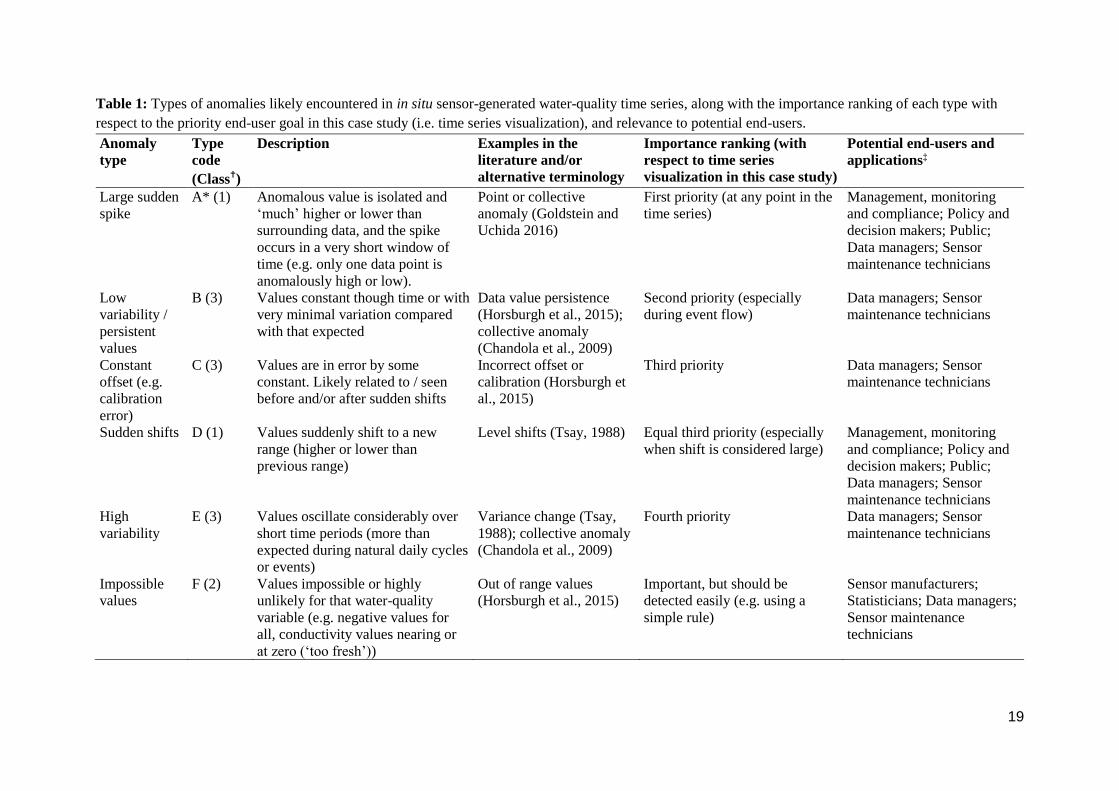
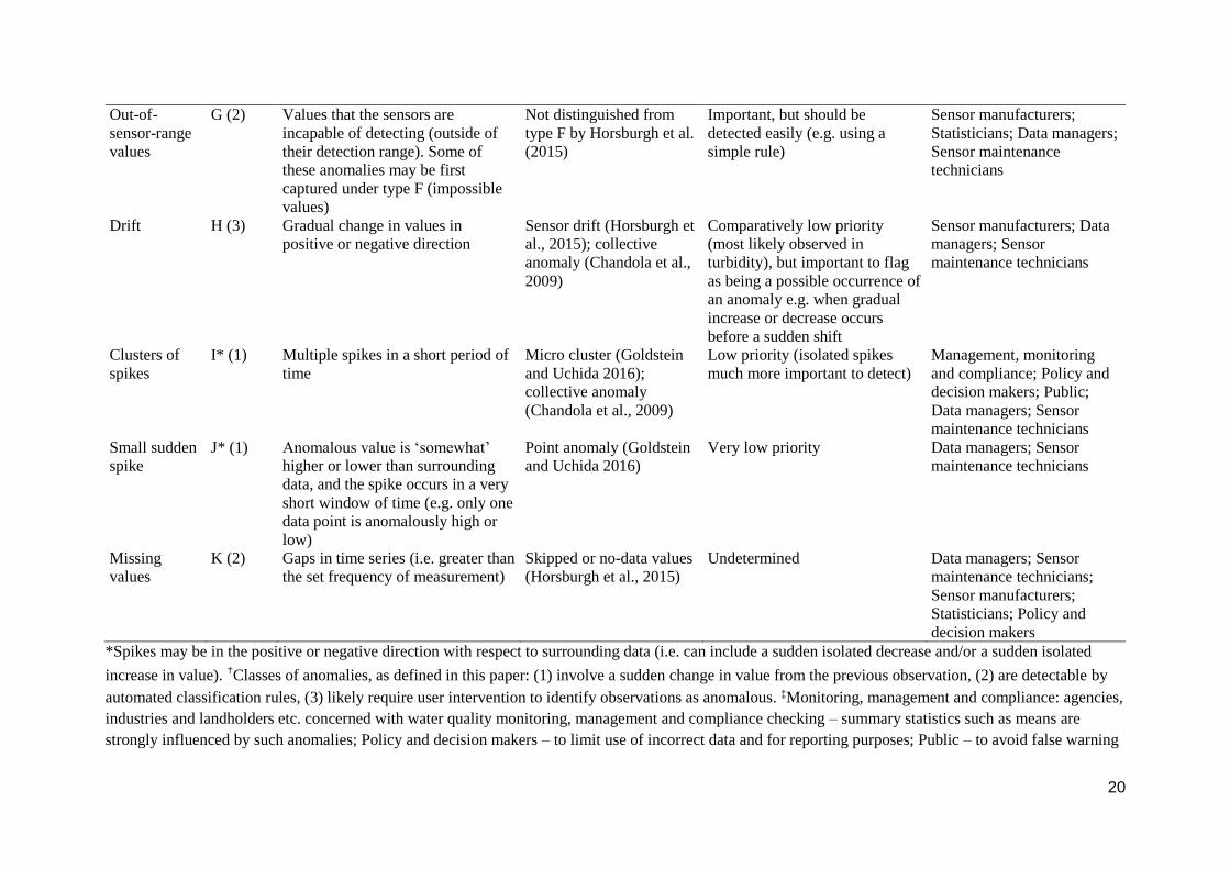
Table 1: Types of anomalies likely encountered in in situ sensor-generated water-quality time series, along with the importance ranking of each type with

respect to the priority end-user goal in this case study (i.e. time series visualization), and relevance to potential end-users.

Anomaly

type

Type

code

(Class✝)

Description Examples in the

literature and/or

alternative terminology

Importance ranking (with

respect to time series

visualization in this case study)

Potential end-users and

applications‡

Large sudden

spike

A* (1) Anomalous value is isolated and

‘much’ higher or lower than

surrounding data, and the spike

occurs in a very short window of

time (e.g. only one data point is

anomalously high or low).

Point or collective

anomaly (Goldstein and

Uchida 2016)

First priority (at any point in the

time series)

Management, monitoring

and compliance; Policy and

decision makers; Public;

Data managers; Sensor

maintenance technicians

Low

variability /

persistent

values

B (3) Values constant though time or with

very minimal variation compared

with that expected

Data value persistence

(Horsburgh et al., 2015);

collective anomaly

(Chandola et al., 2009)

Second priority (especially

during event flow)

Data managers; Sensor

maintenance technicians

Constant

offset (e.g.

calibration

error)

C (3) Values are in error by some

constant. Likely related to / seen

before and/or after sudden shifts

Incorrect offset or

calibration (Horsburgh et

al., 2015)

Third priority Data managers; Sensor

maintenance technicians

Sudden shifts D (1) Values suddenly shift to a new

range (higher or lower than

previous range)

Level shifts (Tsay, 1988) Equal third priority (especially

when shift is considered large)

Management, monitoring

and compliance; Policy and

decision makers; Public;

Data managers; Sensor

maintenance technicians

High

variability

E (3) Values oscillate considerably over

short time periods (more than

expected during natural daily cycles

or events)

Variance change (Tsay,

1988); collective anomaly

(Chandola et al., 2009)

Fourth priority Data managers; Sensor

maintenance technicians

Impossible

values

F (2) Values impossible or highly

unlikely for that water-quality

variable (e.g. negative values for

all, conductivity values nearing or

at zero (‘too fresh’))

Out of range values

(Horsburgh et al., 2015)

Important, but should be

detected easily (e.g. using a

simple rule)

Sensor manufacturers;

Statisticians; Data managers;

Sensor maintenance

technicians

20

Out-of-

sensor-range

values

G (2) Values that the sensors are

incapable of detecting (outside of

their detection range). Some of

these anomalies may be first

captured under type F (impossible

values)

Not distinguished from

type F by Horsburgh et al.

(2015)

Important, but should be

detected easily (e.g. using a

simple rule)

Sensor manufacturers;

Statisticians; Data managers;

Sensor maintenance

technicians

Drift H (3) Gradual change in values in

positive or negative direction

Sensor drift (Horsburgh et

al., 2015); collective

anomaly (Chandola et al.,

2009)

Comparatively low priority

(most likely observed in

turbidity), but important to flag

as being a possible occurrence of

an anomaly e.g. when gradual

increase or decrease occurs

before a sudden shift

Sensor manufacturers; Data

managers; Sensor

maintenance technicians

Clusters of

spikes

I* (1) Multiple spikes in a short period of

time

Micro cluster (Goldstein

and Uchida 2016);

collective anomaly

(Chandola et al., 2009)

Low priority (isolated spikes

much more important to detect)

Management, monitoring

and compliance; Policy and

decision makers; Public;

Data managers; Sensor

maintenance technicians

Small sudden

spike

J* (1) Anomalous value is ‘somewhat’

higher or lower than surrounding

data, and the spike occurs in a very

short window of time (e.g. only one

data point is anomalously high or

low)

Point anomaly (Goldstein

and Uchida 2016)

Very low priority Data managers; Sensor

maintenance technicians

Missing

values

K (2) Gaps in time series (i.e. greater than

the set frequency of measurement)

Skipped or no-data values

(Horsburgh et al., 2015)

Undetermined Data managers; Sensor

maintenance technicians;

Sensor manufacturers;

Statisticians; Policy and

decision makers

*Spikes may be in the positive or negative direction with respect to surrounding data (i.e. can include a sudden isolated decrease and/or a sudden isolated

increase in value). ✝Classes of anomalies, as defined in this paper: (1) involve a sudden change in value from the previous observation, (2) are detectable by

automated classification rules, (3) likely require user intervention to identify observations as anomalous. ‡Monitoring, management and compliance: agencies,

industries and landholders etc. concerned with water quality monitoring, management and compliance checking – summary statistics such as means are

strongly influenced by such anomalies; Policy and decision makers – to limit use of incorrect data and for reporting purposes; Public – to avoid false warning

21

of water quality breaches; Data managers – for quality control and assurance and to increase confidence in the data by reporting the presence of such

anomalies; Sensor maintenance technicians – to ensure timely and correct calibration and maintenance of equipment; Sensor manufacturers – to improve

performance, e.g. extend battery life, improve wiper quality to further minimise biofouling; Statisticians – for AD methods to better detect other non-trivial

anomaly types and/or for methods requiring regular and frequent observations.

22

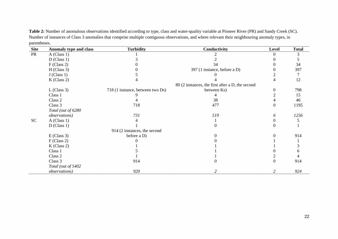
Table 2: Number of anomalous observations identified according to type, class and water-quality variable at Pioneer River (PR) and Sandy Creek (SC).

Number of instances of Class 3 anomalies that comprise multiple contiguous observations, and where relevant their neighbouring anomaly types, in

parentheses.

Site Anomaly type and class Turbidity Conductivity Level Total

PR A (Class 1) 1 2 0 3

D (Class 1) 3 2 0 5

F (Class 2) 0 34 0 34

H (Class 3) 0 397 (1 instance, before a D) 0 397

J (Class 1) 5 0 2 7

K (Class 2) 4 4 4 12

L (Class 3) 718 (1 instance, between two Ds)

80 (2 instances, the first after a D, the second

between Ks) 0 798

Class 1 9 4 2 15

Class 2 4 38 4 46

Class 3 718 477 0 1195

Total (out of 6280

observations) 731 519 6 1256

SC A (Class 1) 4 1 0 5

D (Class 1) 1 0 0 1

E (Class 3)

914 (2 instances, the second

before a D) 0 0 914

F (Class 2) 0 0 1 1

K (Class 2) 1 1 1 3

Class 1 5 1 0 6

Class 2 1 1 2 4

Class 3 914 0 0 914

Total (out of 5402

observations) 920 2 2 924

23

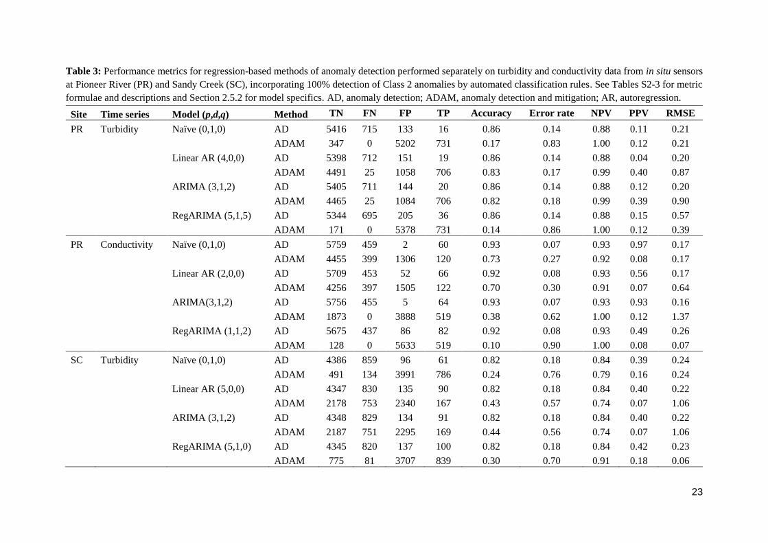
Table 3: Performance metrics for regression-based methods of anomaly detection performed separately on turbidity and conductivity data from in situ sensors

at Pioneer River (PR) and Sandy Creek (SC), incorporating 100% detection of Class 2 anomalies by automated classification rules. See Tables S2-3 for metric

formulae and descriptions and Section 2.5.2 for model specifics. AD, anomaly detection; ADAM, anomaly detection and mitigation; AR, autoregression.

Site Time series Model (p,d,q) Method TN FN FP TP Accuracy Error rate NPV PPV RMSE

PR Turbidity Naïve (0,1,0) AD 5416 715 133 16 0.86 0.14 0.88 0.11 0.21

ADAM 347 0 5202 731 0.17 0.83 1.00 0.12 0.21

Linear AR (4,0,0) AD 5398 712 151 19 0.86 0.14 0.88 0.04 0.20

ADAM 4491 25 1058 706 0.83 0.17 0.99 0.40 0.87

ARIMA (3,1,2) AD 5405 711 144 20 0.86 0.14 0.88 0.12 0.20

ADAM 4465 25 1084 706 0.82 0.18 0.99 0.39 0.90

RegARIMA (5,1,5) AD 5344 695 205 36 0.86 0.14 0.88 0.15 0.57

ADAM 171 0 5378 731 0.14 0.86 1.00 0.12 0.39

PR Conductivity Naïve (0,1,0) AD 5759 459 2 60 0.93 0.07 0.93 0.97 0.17

ADAM 4455 399 1306 120 0.73 0.27 0.92 0.08 0.17

Linear AR (2,0,0) AD 5709 453 52 66 0.92 0.08 0.93 0.56 0.17

ADAM 4256 397 1505 122 0.70 0.30 0.91 0.07 0.64

ARIMA(3,1,2) AD 5756 455 5 64 0.93 0.07 0.93 0.93 0.16

ADAM 1873 0 3888 519 0.38 0.62 1.00 0.12 1.37

RegARIMA (1,1,2) AD 5675 437 86 82 0.92 0.08 0.93 0.49 0.26

ADAM 128 0 5633 519 0.10 0.90 1.00 0.08 0.07

SC Turbidity Naïve (0,1,0) AD 4386 859 96 61 0.82 0.18 0.84 0.39 0.24

ADAM 491 134 3991 786 0.24 0.76 0.79 0.16 0.24

Linear AR (5,0,0) AD 4347 830 135 90 0.82 0.18 0.84 0.40 0.22

ADAM 2178 753 2340 167 0.43 0.57 0.74 0.07 1.06

ARIMA (3,1,2) AD 4348 829 134 91 0.82 0.18 0.84 0.40 0.22

ADAM 2187 751 2295 169 0.44 0.56 0.74 0.07 1.06

RegARIMA (5,1,0) AD 4345 820 137 100 0.82 0.18 0.84 0.42 0.23

ADAM 775 81 3707 839 0.30 0.70 0.91 0.18 0.06

24

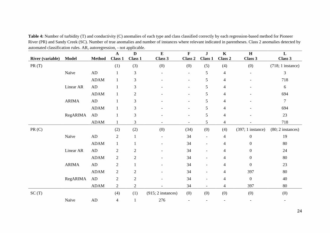
Table 4: Number of turbidity (T) and conductivity (C) anomalies of each type and class classified correctly by each regression-based method for Pioneer

River (PR) and Sandy Creek (SC). Number of true anomalies and number of instances where relevant indicated in parentheses. Class 2 anomalies detected by

automated classification rules. AR, autoregression, - not applicable.

River (variable) Model Method

A

Class 1

D

Class 1

E

Class 3

F

Class 2

J

Class 1

K

Class 2

H

Class 3

L

Class 3

PR (T) (1) (3) (0) (0) (5) (4) (0) (718; 1 instance)

Naïve AD 1 3 - - 5 4 - 3

ADAM 1 3 - - 5 4 - 718

Linear AR AD 1 3 - - 5 4 - 6

ADAM 1 2 - - 5 4 - 694

ARIMA AD 1 3 - - 5 4 - 7

ADAM 1 3 - - 5 4 - 694

RegARIMA AD 1 3 - - 5 4 - 23

ADAM 1 3 - - 5 4 - 718

PR (C) (2) (2) (0) (34) (0) (4) (397; 1 instance) (80; 2 instances)

Naïve AD 2 1 - 34 - 4 0 19

ADAM 1 1 - 34 - 4 0 80

Linear AR AD 2 2 - 34 - 4 0 24

ADAM 2 2 - 34 - 4 0 80

ARIMA AD 2 1 - 34 - 4 0 23

ADAM 2 2 - 34 - 4 397 80

RegARIMA AD 2 2 - 34 - 4 0 40

ADAM 2 2 - 34 - 4 397 80

SC (T) (4) (1) (915; 2 instances) (0) (0) (0) (0) (0)

Naïve AD 4 1 276 - - - - -

25

ADAM 4 1 780 - - - - -

Linear AR AD 4 0 85 - - - - -

ADAM 4 1 161 - - - - -

ARIMA AD 4 0 85 - - - - -

ADAM 4 1 162 - - - - -

RegARIMA AD 4 1 94 - - - - -

ADAM 4 1 833 - - - - -

SC (C) (1) (1) (0) (0) (0) (0) (0) (0)

Naïve AD 1 1 - - - - - -

ADAM 1 1 - - - - - -

Linear AR AD 1 1 - - - - - -

ADAM 1 1 - - - - - -

ARIMA AD 1 1 - - - - - -

ADAM 1 1 - - - - - -

RegARIMA AD 1 1 - - - - - -

ADAM 1 1 - - - - - -

26

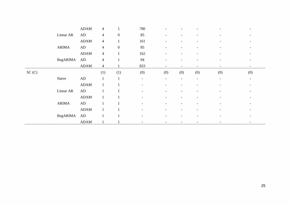
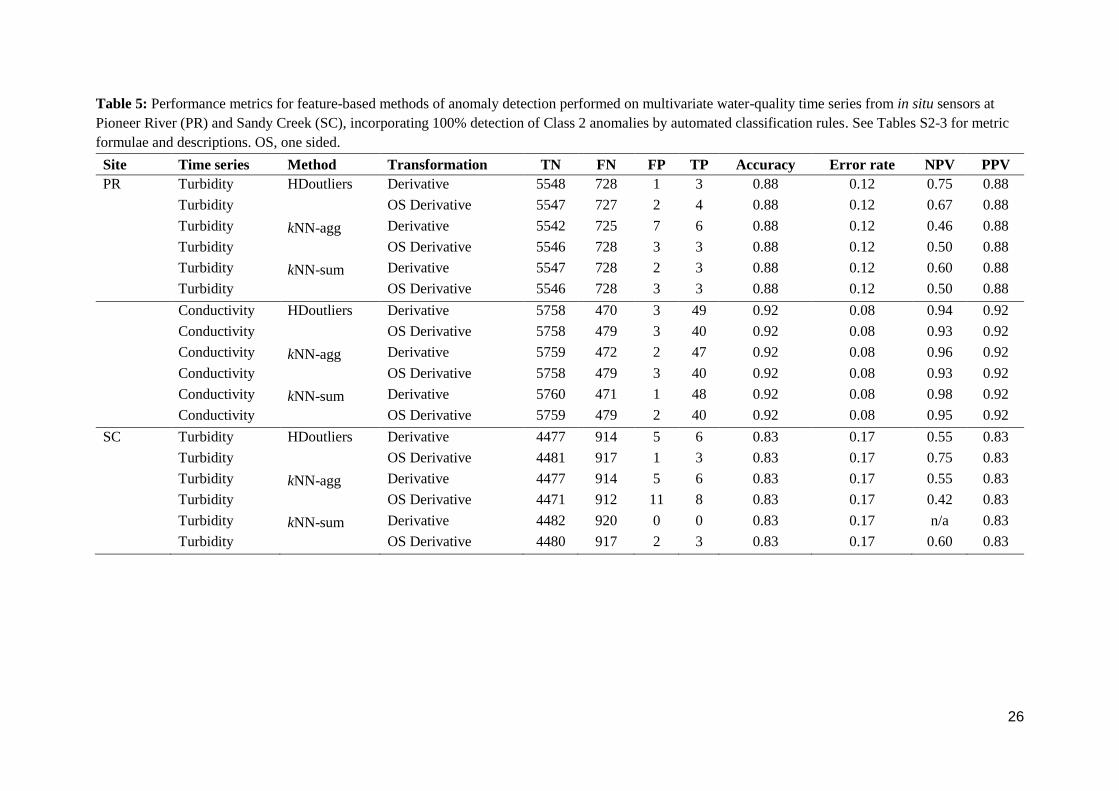
Table 5: Performance metrics for feature-based methods of anomaly detection performed on multivariate water-quality time series from in situ sensors at

Pioneer River (PR) and Sandy Creek (SC), incorporating 100% detection of Class 2 anomalies by automated classification rules. See Tables S2-3 for metric

formulae and descriptions. OS, one sided.

Site Time series Method Transformation TN FN FP TP Accuracy Error rate NPV PPV

PR Turbidity HDoutliers Derivative 5548 728 1 3 0.88 0.12 0.75 0.88

Turbidity OS Derivative 5547 727 2 4 0.88 0.12 0.67 0.88

Turbidity kNN-agg Derivative 5542 725 7 6 0.88 0.12 0.46 0.88

Turbidity OS Derivative 5546 728 3 3 0.88 0.12 0.50 0.88

Turbidity kNN-sum Derivative 5547 728 2 3 0.88 0.12 0.60 0.88

Turbidity OS Derivative 5546 728 3 3 0.88 0.12 0.50 0.88

Conductivity HDoutliers Derivative 5758 470 3 49 0.92 0.08 0.94 0.92

Conductivity OS Derivative 5758 479 3 40 0.92 0.08 0.93 0.92

Conductivity kNN-agg Derivative 5759 472 2 47 0.92 0.08 0.96 0.92

Conductivity OS Derivative 5758 479 3 40 0.92 0.08 0.93 0.92

Conductivity kNN-sum Derivative 5760 471 1 48 0.92 0.08 0.98 0.92

Conductivity OS Derivative 5759 479 2 40 0.92 0.08 0.95 0.92

SC Turbidity HDoutliers Derivative 4477 914 5 6 0.83 0.17 0.55 0.83

Turbidity OS Derivative 4481 917 1 3 0.83 0.17 0.75 0.83

Turbidity kNN-agg Derivative 4477 914 5 6 0.83 0.17 0.55 0.83

Turbidity OS Derivative 4471 912 11 8 0.83 0.17 0.42 0.83

Turbidity kNN-sum Derivative 4482 920 0 0 0.83 0.17 n/a 0.83

Turbidity OS Derivative 4480 917 2 3 0.83 0.17 0.60 0.83

27

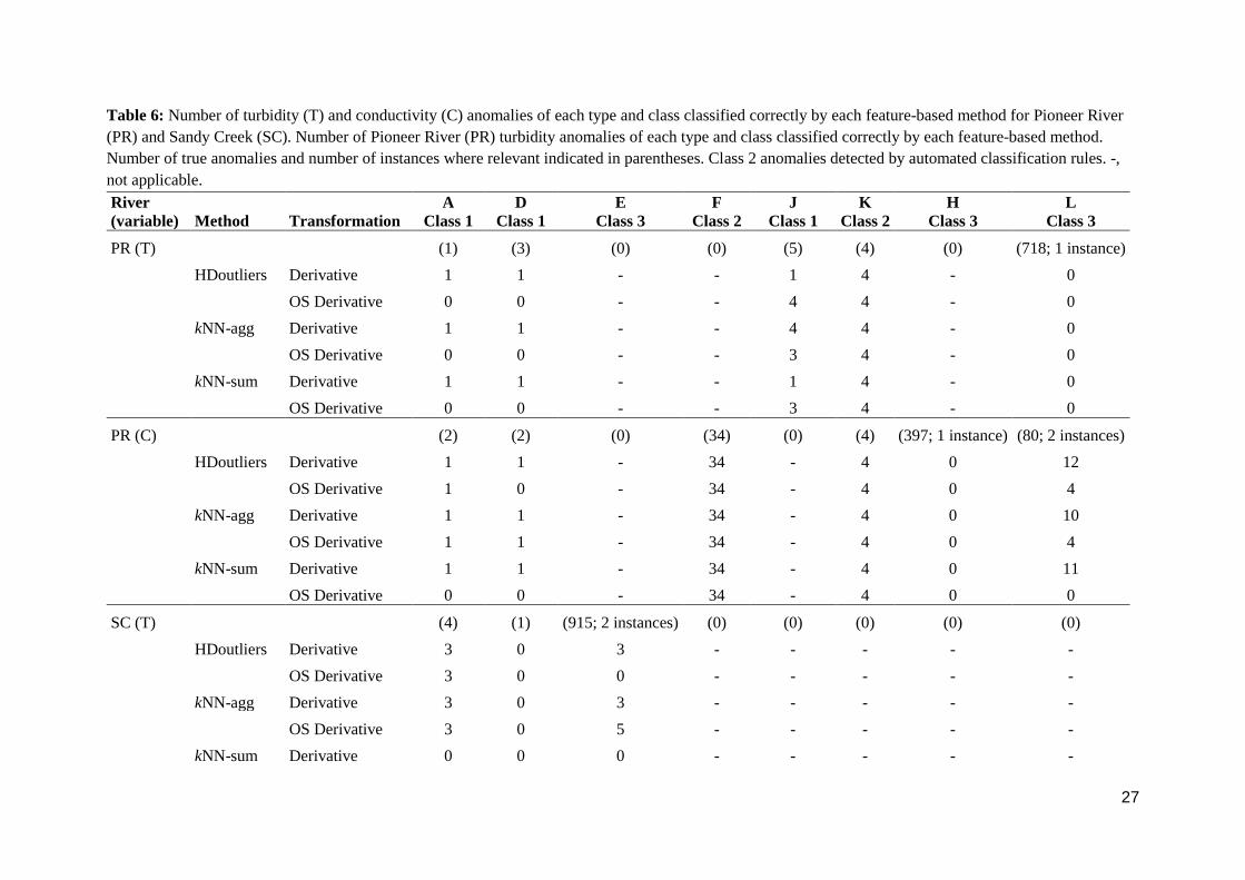
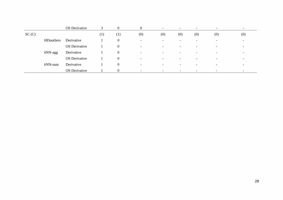
Table 6: Number of turbidity (T) and conductivity (C) anomalies of each type and class classified correctly by each feature-based method for Pioneer River

(PR) and Sandy Creek (SC). Number of Pioneer River (PR) turbidity anomalies of each type and class classified correctly by each feature-based method.

Number of true anomalies and number of instances where relevant indicated in parentheses. Class 2 anomalies detected by automated classification rules. -,

not applicable.

River

(variable) Method Transformation

A

Class 1

D

Class 1

E

Class 3

F

Class 2

J

Class 1

K

Class 2

H

Class 3

L

Class 3

PR (T) (1) (3) (0) (0) (5) (4) (0) (718; 1 instance)

HDoutliers Derivative 1 1 - - 1 4 - 0

OS Derivative 0 0 - - 4 4 - 0

kNN-agg Derivative 1 1 - - 4 4 - 0

OS Derivative 0 0 - - 3 4 - 0

kNN-sum Derivative 1 1 - - 1 4 - 0

OS Derivative 0 0 - - 3 4 - 0

PR (C) (2) (2) (0) (34) (0) (4) (397; 1 instance) (80; 2 instances)

HDoutliers Derivative 1 1 - 34 - 4 0 12

OS Derivative 1 0 - 34 - 4 0 4

kNN-agg Derivative 1 1 - 34 - 4 0 10

OS Derivative 1 1 - 34 - 4 0 4

kNN-sum Derivative 1 1 - 34 - 4 0 11

OS Derivative 0 0 - 34 - 4 0 0

SC (T) (4) (1) (915; 2 instances) (0) (0) (0) (0) (0)

HDoutliers Derivative 3 0 3 - - - - -

OS Derivative 3 0 0 - - - - -

kNN-agg Derivative 3 0 3 - - - - -

OS Derivative 3 0 5 - - - - -

kNN-sum Derivative 0 0 0 - - - - -

28

OS Derivative 3 0 0 - - - - -

SC (C) (1) (1) (0) (0) (0) (0) (0) (0)

HDoutliers Derivative 1 0 - - - - - -

OS Derivative 1 0 - - - - - -

kNN-agg Derivative 1 0 - - - - - -

OS Derivative 1 0 - - - - - -

kNN-sum Derivative 1 0 - - - - - -

OS Derivative 1 0 - - - - - -

29

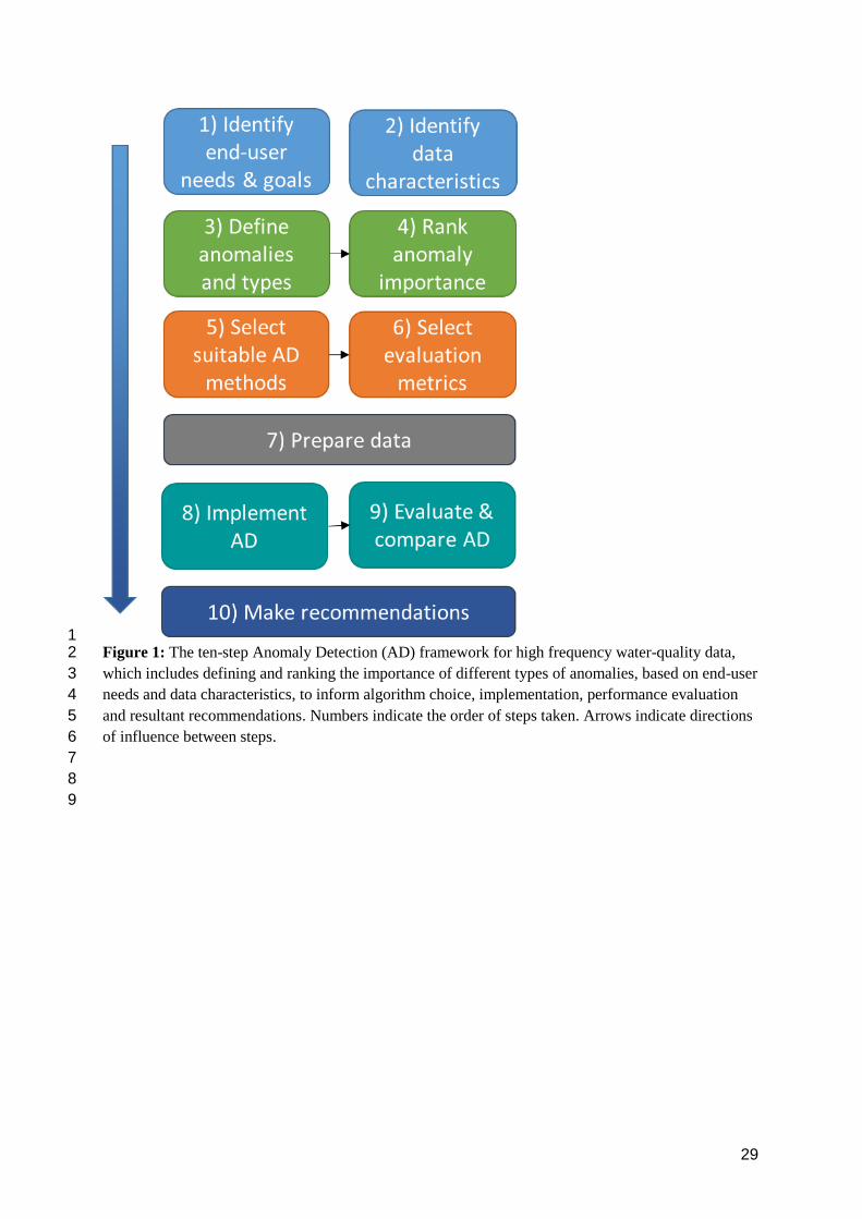
1 Figure 1: The ten-step Anomaly Detection (AD) framework for high frequency water-quality data, 2

which includes defining and ranking the importance of different types of anomalies, based on end-user 3

needs and data characteristics, to inform algorithm choice, implementation, performance evaluation 4

and resultant recommendations. Numbers indicate the order of steps taken. Arrows indicate directions 5

of influence between steps. 6

7

8

9

1

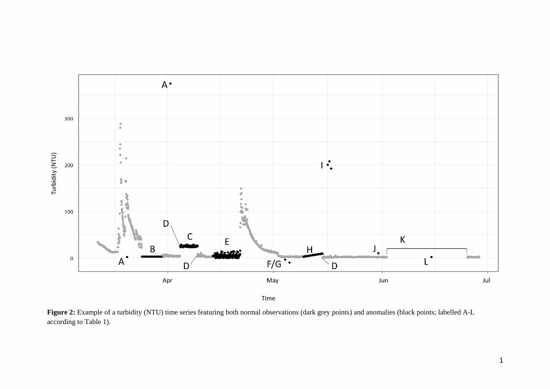
Figure 2: Example of a turbidity (NTU) time series featuring both normal observations (dark grey points) and anomalies (black points; labelled A-L

according to Table 1).

2

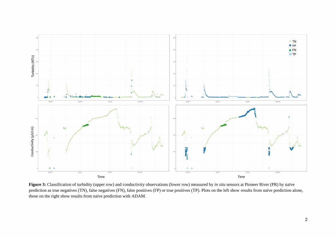
Figure 3: Classification of turbidity (upper row) and conductivity observations (lower row) measured by in situ sensors at Pioneer River (PR) by naïve

prediction as true negatives (TN), false negatives (FN), false positives (FP) or true positives (TP). Plots on the left show results from naïve prediction alone,

those on the right show results from naïve prediction with ADAM.

3

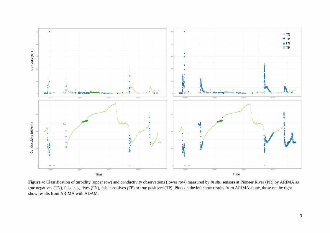
Figure 4: Classification of turbidity (upper row) and conductivity observations (lower row) measured by in situ sensors at Pioneer River (PR) by ARIMA as

true negatives (TN), false negatives (FN), false positives (FP) or true positives (TP). Plots on the left show results from ARIMA alone, those on the right

show results from ARIMA with ADAM.

4

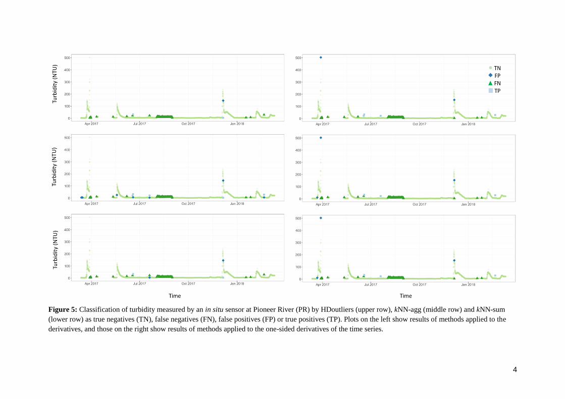
Figure 5: Classification of turbidity measured by an in situ sensor at Pioneer River (PR) by HDoutliers (upper row), kNN-agg (middle row) and kNN-sum

(lower row) as true negatives (TN), false negatives (FN), false positives (FP) or true positives (TP). Plots on the left show results of methods applied to the

derivatives, and those on the right show results of methods applied to the one-sided derivatives of the time series.

1

Supplementary materials

The supplementary materials for the article by Leigh et al. “A framework for automated anomaly

detection in high frequency water-quality data from in situ sensors” comprise the following:

1. Bivariate relationships and time series showing anomalous and non-anomalous observations

for water quality data collected from Pioneer River and Sandy Creek (Figures S1-3)

2. Results of the regression-based and feature-based methods applied to the conductivity time

series at Sandy Creek (Tables S1-5);

3. Time series plots not included in the main article that show the observations classified as true

positives, false positives, true negatives or false negatives according to each method applied to

each time series of water-quality data at each site (Figures S4-S12);

4. Diagnostic plots for the regression-based methods requiring training that were implemented in

the main article (Figures S13-20);

5. Files (supplied separately) containing the time series data, supplied by the Queensland

Department of Environment and Science (please refer to the Department's website for the

disclaimer to these data: https://www.des.qld.gov.au/legal/disclaimer/), and the anomaly-type

coding used in the main article (data_pioneer.csv and data_sandy.csv); and

6. Files (supplied separately) containing the R code used to implement the regression-based

methods on the time series data, and to calculate performance metrics, as outlined in the main

article (PioneerRiver.R, SandyCreek.R, NaivePredictor.R, Prediction.R and

ADPerformance.R).

2

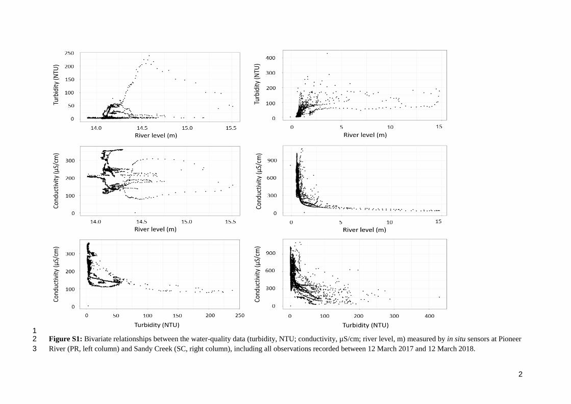
1 Figure S1: Bivariate relationships between the water-quality data (turbidity, NTU; conductivity, µS/cm; river level, m) measured by in situ sensors at Pioneer 2

River (PR, left column) and Sandy Creek (SC, right column), including all observations recorded between 12 March 2017 and 12 March 2018. 3

3

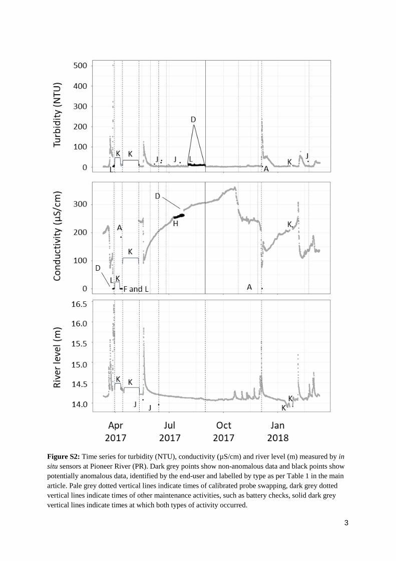
Figure S2: Time series for turbidity (NTU), conductivity (µS/cm) and river level (m) measured by in

situ sensors at Pioneer River (PR). Dark grey points show non-anomalous data and black points show

potentially anomalous data, identified by the end-user and labelled by type as per Table 1 in the main

article. Pale grey dotted vertical lines indicate times of calibrated probe swapping, dark grey dotted

vertical lines indicate times of other maintenance activities, such as battery checks, solid dark grey

vertical lines indicate times at which both types of activity occurred.

4

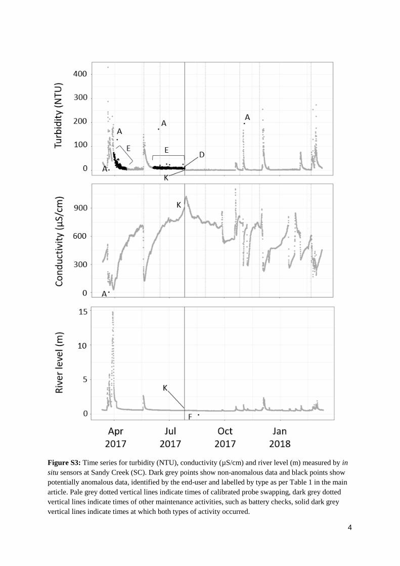
Figure S3: Time series for turbidity (NTU), conductivity (µS/cm) and river level (m) measured by in

situ sensors at Sandy Creek (SC). Dark grey points show non-anomalous data and black points show

potentially anomalous data, identified by the end-user and labelled by type as per Table 1 in the main

article. Pale grey dotted vertical lines indicate times of calibrated probe swapping, dark grey dotted

vertical lines indicate times of other maintenance activities, such as battery checks, solid dark grey

vertical lines indicate times at which both types of activity occurred.

5

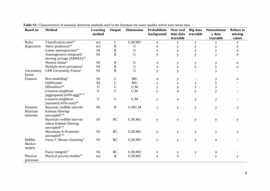
Table S1: Characteristics of anomaly detection methods used in the literature for water quality and/or time series data.

Based on Method Learning

method

Output Dimensions Probabilistic

background

Near-real

time data

tractable

Big-data

tractable

Nonstationar

y data

tractable

Robust to

missing

values

Rules Classification rules*1 n/a C U,M,MU n y y y y

Regression Naïve prediction*2 n/a R U n y y y n

Linear autoregression*2 SS R U n y y y n

Autoregressive integrated

moving average (ARIMA)*2

SS R U n y y y n

Nearest cluster2 SS R U n y y y n

Multiple-level perceptron2 SS R U n y y y n

Uncertainty

fusion

GPR Uncertainty Fusion3 SS R U y y - y -

Features Box-modelling4 SS C MU n y - y n

OddStream5 SS C MU y y y y -

HDoutliers*6 U C U,M y n y y -

k-nearest neighbour

(aggregated) (kNN-agg)*7,8

U C U,M y n y y -

k-nearest neighbour

(summed) kNN-sum)*8

U C U,M y n y y -

Dynamic

Bayesian

networks

Bayesian credible interval-

Kalman filtering-

uncoupled9,10

SS R U,MU,M y y y y y

Bayesian credible interval-

robust Kalman filtering-

uncoupled9,10

SS RC U,M,MU y y y y y

Maximum-A-Posteriori-

uncoupled9,10

SS RC U,M,MU y y y y y

Hidden

Markov

models

Fuzzy C-Means clustering11 SS RC U,M,MU y y y n -

Fuzzy integrals11 SS RC U,M,MU y y y n -

Physical

processes

Physical process models12 n/a R U,M,MU n n - y y

6

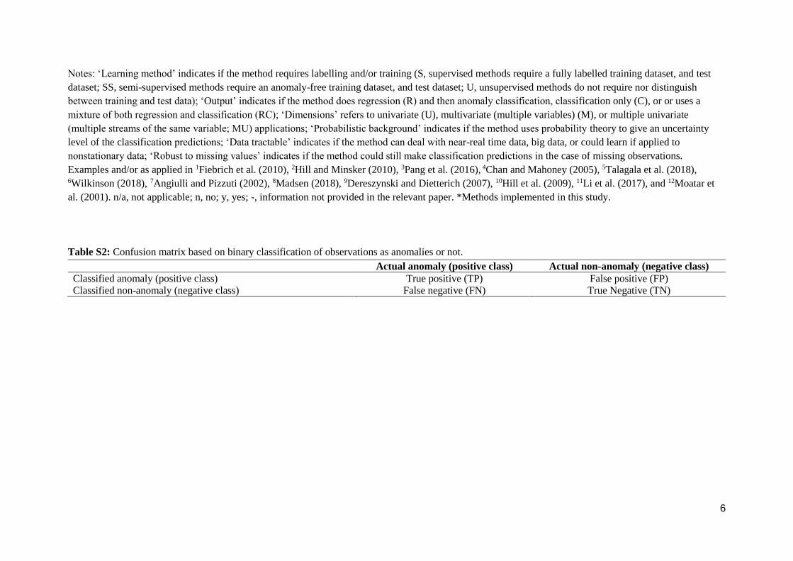
Notes: ‘Learning method’ indicates if the method requires labelling and/or training (S, supervised methods require a fully labelled training dataset, and test

dataset; SS, semi-supervised methods require an anomaly-free training dataset, and test dataset; U, unsupervised methods do not require nor distinguish

between training and test data); ‘Output’ indicates if the method does regression (R) and then anomaly classification, classification only (C), or or uses a

mixture of both regression and classification (RC); ‘Dimensions’ refers to univariate (U), multivariate (multiple variables) (M), or multiple univariate

(multiple streams of the same variable; MU) applications; ‘Probabilistic background’ indicates if the method uses probability theory to give an uncertainty

level of the classification predictions; ‘Data tractable’ indicates if the method can deal with near-real time data, big data, or could learn if applied to

nonstationary data; ‘Robust to missing values’ indicates if the method could still make classification predictions in the case of missing observations.

Examples and/or as applied in 1Fiebrich et al. (2010), 2Hill and Minsker (2010), 3Pang et al. (2016), 4Chan and Mahoney (2005), 5Talagala et al. (2018), 6Wilkinson (2018), 7Angiulli and Pizzuti (2002), 8Madsen (2018), 9Dereszynski and Dietterich (2007), 10Hill et al. (2009), 11Li et al. (2017), and 12Moatar et

al. (2001). n/a, not applicable; n, no; y, yes; -, information not provided in the relevant paper. *Methods implemented in this study.

Table S2: Confusion matrix based on binary classification of observations as anomalies or not.

Actual anomaly (positive class) Actual non-anomaly (negative class)

Classified anomaly (positive class) True positive (TP) False positive (FP)

Classified non-anomaly (negative class) False negative (FN) True Negative (TN)

7

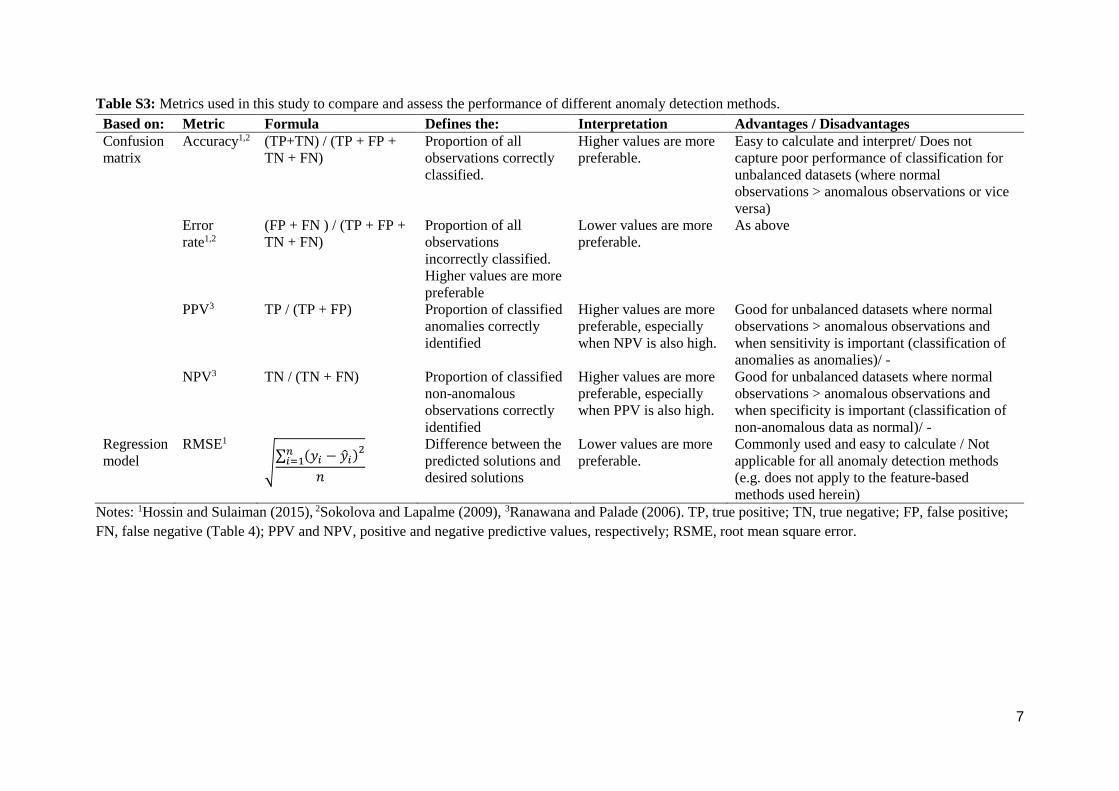
Table S3: Metrics used in this study to compare and assess the performance of different anomaly detection methods.

Based on: Metric Formula Defines the: Interpretation Advantages / Disadvantages

Confusion

matrix

Accuracy1,2 (TP+TN) / (TP + FP +

TN + FN)

Proportion of all

observations correctly

classified.

Higher values are more

preferable.

Easy to calculate and interpret/ Does not

capture poor performance of classification for

unbalanced datasets (where normal

observations > anomalous observations or vice

versa)

Error

rate1,2

(FP + FN ) / (TP + FP +

TN + FN)

Proportion of all

observations

incorrectly classified.

Higher values are more

preferable

Lower values are more

preferable.

As above

PPV3 TP / (TP + FP) Proportion of classified

anomalies correctly

identified

Higher values are more

preferable, especially

when NPV is also high.

Good for unbalanced datasets where normal

observations > anomalous observations and

when sensitivity is important (classification of

anomalies as anomalies)/ -

NPV3 TN / (TN + FN) Proportion of classified

non-anomalous

observations correctly

identified

Higher values are more

preferable, especially

when PPV is also high.

Good for unbalanced datasets where normal

observations > anomalous observations and

when specificity is important (classification of

non-anomalous data as normal)/ -

Regression

model

RMSE1

√∑ (𝑦𝑖 − �̂�𝑖)𝑛

𝑖=12

𝑛

Difference between the

predicted solutions and

desired solutions

Lower values are more

preferable.

Commonly used and easy to calculate / Not

applicable for all anomaly detection methods

(e.g. does not apply to the feature-based

methods used herein)

Notes: 1Hossin and Sulaiman (2015), 2Sokolova and Lapalme (2009), 3Ranawana and Palade (2006). TP, true positive; TN, true negative; FP, false positive;

FN, false negative (Table 4); PPV and NPV, positive and negative predictive values, respectively; RSME, root mean square error.

8

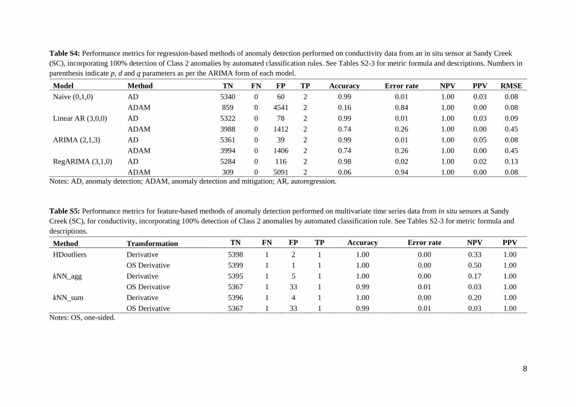
Table S4: Performance metrics for regression-based methods of anomaly detection performed on conductivity data from an in situ sensor at Sandy Creek

(SC), incorporating 100% detection of Class 2 anomalies by automated classification rules. See Tables S2-3 for metric formula and descriptions. Numbers in

parenthesis indicate p, d and q parameters as per the ARIMA form of each model.

Model Method TN FN FP TP Accuracy Error rate NPV PPV RMSE

Naïve (0,1,0) AD 5340 0 60 2 0.99 0.01 1.00 0.03 0.08

ADAM 859 0 4541 2 0.16 0.84 1.00 0.00 0.08

Linear AR (3,0,0) AD 5322 0 78 2 0.99 0.01 1.00 0.03 0.09

ADAM 3988 0 1412 2 0.74 0.26 1.00 0.00 0.45

ARIMA (2,1,3) AD 5361 0 39 2 0.99 0.01 1.00 0.05 0.08

ADAM 3994 0 1406 2 0.74 0.26 1.00 0.00 0.45

RegARIMA (3,1,0) AD 5284 0 116 2 0.98 0.02 1.00 0.02 0.13

ADAM 309 0 5091 2 0.06 0.94 1.00 0.00 0.08

Notes: AD, anomaly detection; ADAM, anomaly detection and mitigation; AR, autoregression.

Table S5: Performance metrics for feature-based methods of anomaly detection performed on multivariate time series data from in situ sensors at Sandy

Creek (SC), for conductivity, incorporating 100% detection of Class 2 anomalies by automated classification rule. See Tables S2-3 for metric formula and

descriptions.

Method Transformation TN FN FP TP Accuracy Error rate NPV PPV

HDoutliers Derivative 5398 1 2 1 1.00 0.00 0.33 1.00

OS Derivative 5399 1 1 1 1.00 0.00 0.50 1.00

kNN_agg Derivative 5395 1 5 1 1.00 0.00 0.17 1.00

OS Derivative 5367 1 33 1 0.99 0.01 0.03 1.00

kNN_sum Derivative 5396 1 4 1 1.00 0.00 0.20 1.00

OS Derivative 5367 1 33 1 0.99 0.01 0.03 1.00

Notes: OS, one-sided.

9

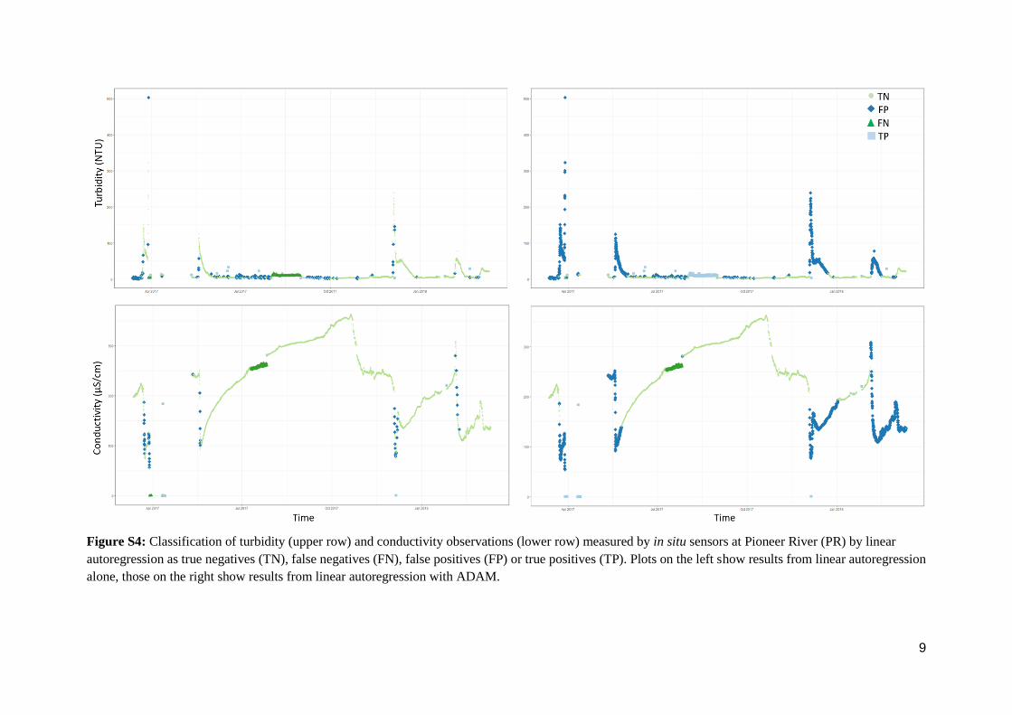
Figure S4: Classification of turbidity (upper row) and conductivity observations (lower row) measured by in situ sensors at Pioneer River (PR) by linear

autoregression as true negatives (TN), false negatives (FN), false positives (FP) or true positives (TP). Plots on the left show results from linear autoregression

alone, those on the right show results from linear autoregression with ADAM.

10

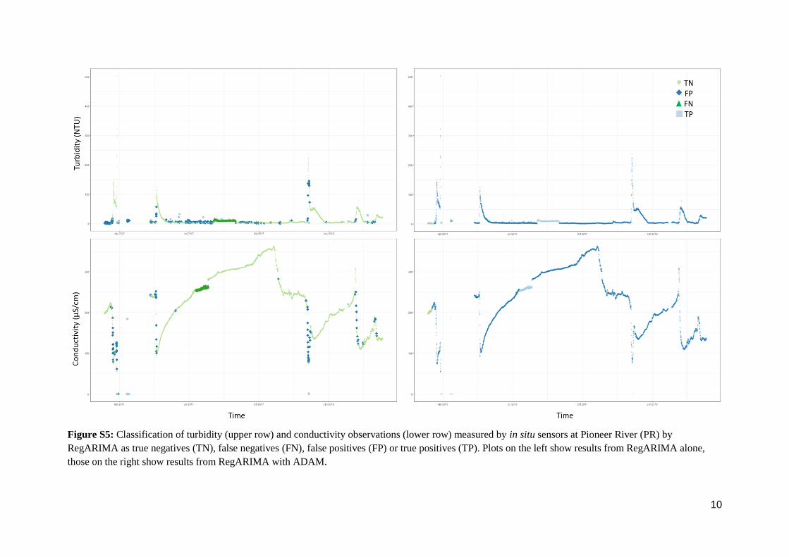
Figure S5: Classification of turbidity (upper row) and conductivity observations (lower row) measured by in situ sensors at Pioneer River (PR) by

RegARIMA as true negatives (TN), false negatives (FN), false positives (FP) or true positives (TP). Plots on the left show results from RegARIMA alone,

those on the right show results from RegARIMA with ADAM.

11

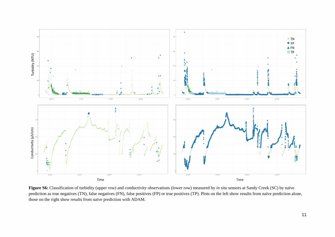
Figure S6: Classification of turbidity (upper row) and conductivity observations (lower row) measured by in situ sensors at Sandy Creek (SC) by naïve

prediction as true negatives (TN), false negatives (FN), false positives (FP) or true positives (TP). Plots on the left show results from naïve prediction alone,

those on the right show results from naïve prediction with ADAM.

12

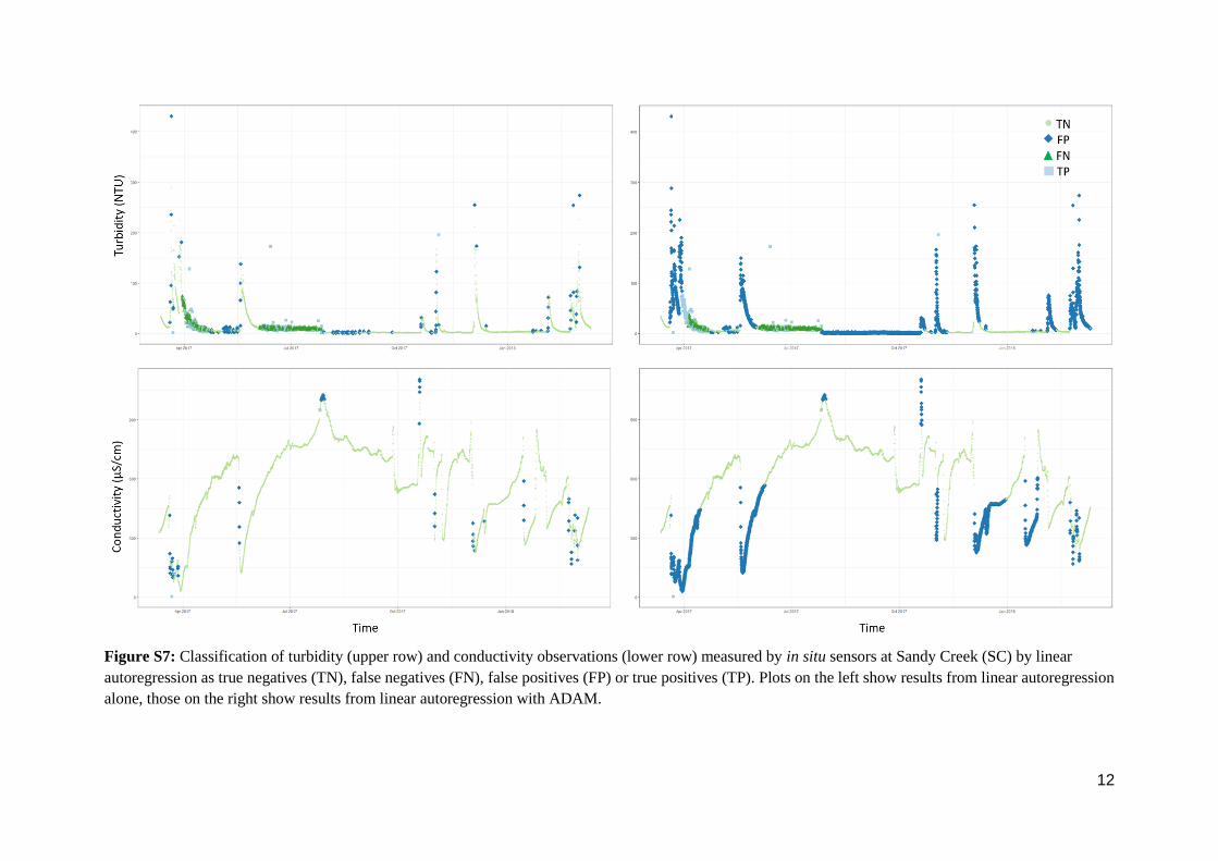
Figure S7: Classification of turbidity (upper row) and conductivity observations (lower row) measured by in situ sensors at Sandy Creek (SC) by linear

autoregression as true negatives (TN), false negatives (FN), false positives (FP) or true positives (TP). Plots on the left show results from linear autoregression

alone, those on the right show results from linear autoregression with ADAM.

13

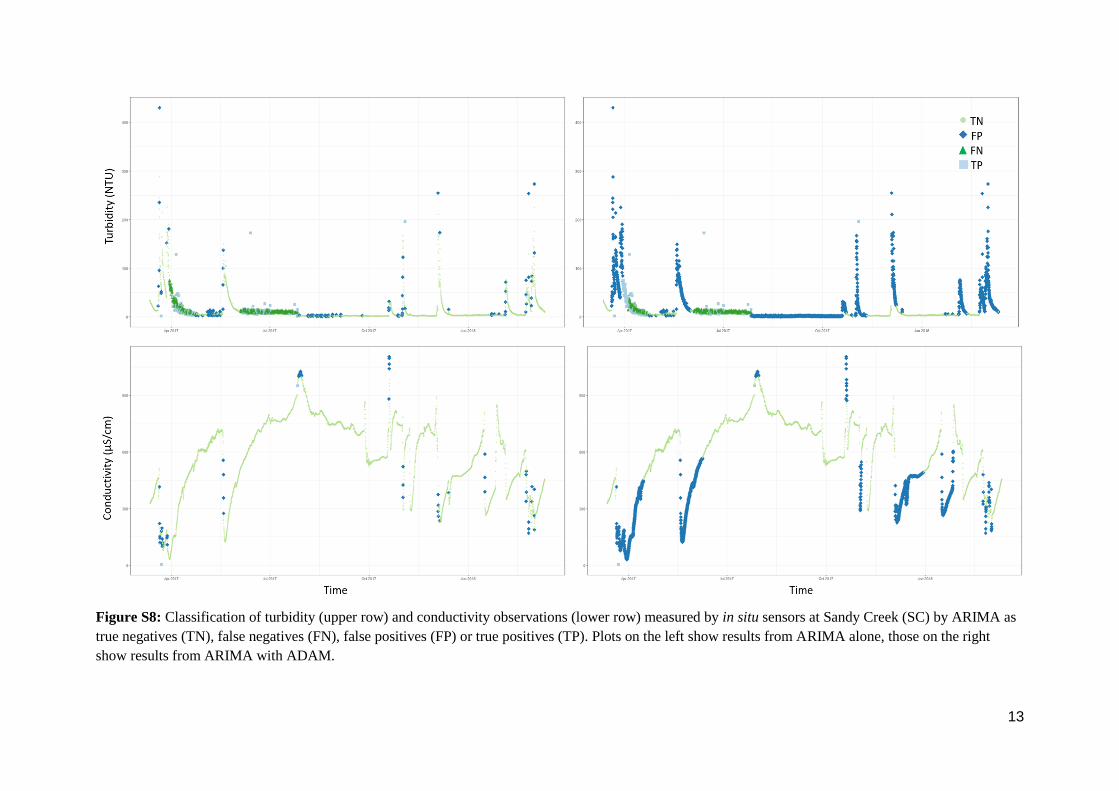
Figure S8: Classification of turbidity (upper row) and conductivity observations (lower row) measured by in situ sensors at Sandy Creek (SC) by ARIMA as

true negatives (TN), false negatives (FN), false positives (FP) or true positives (TP). Plots on the left show results from ARIMA alone, those on the right

show results from ARIMA with ADAM.

14

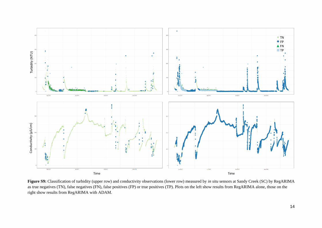
Figure S9: Classification of turbidity (upper row) and conductivity observations (lower row) measured by in situ sensors at Sandy Creek (SC) by RegARIMA

as true negatives (TN), false negatives (FN), false positives (FP) or true positives (TP). Plots on the left show results from RegARIMA alone, those on the

right show results from RegARIMA with ADAM.

15

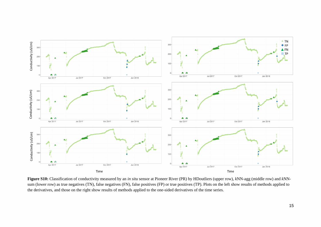
Figure S10: Classification of conductivity measured by an in situ sensor at Pioneer River (PR) by HDoutliers (upper row), kNN-agg (middle row) and kNN-

sum (lower row) as true negatives (TN), false negatives (FN), false positives (FP) or true positives (TP). Plots on the left show results of methods applied to

the derivatives, and those on the right show results of methods applied to the one-sided derivatives of the time series.

16

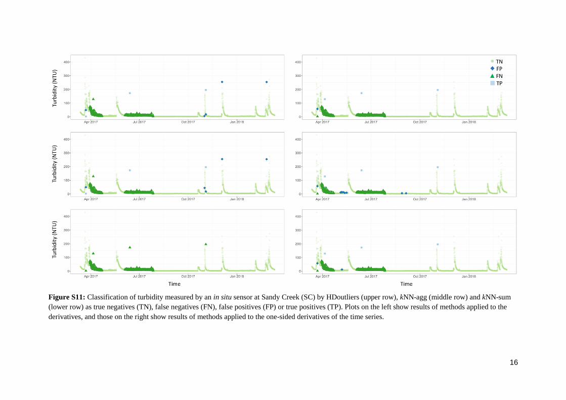
Figure S11: Classification of turbidity measured by an in situ sensor at Sandy Creek (SC) by HDoutliers (upper row), kNN-agg (middle row) and kNN-sum

(lower row) as true negatives (TN), false negatives (FN), false positives (FP) or true positives (TP). Plots on the left show results of methods applied to the

derivatives, and those on the right show results of methods applied to the one-sided derivatives of the time series.

17

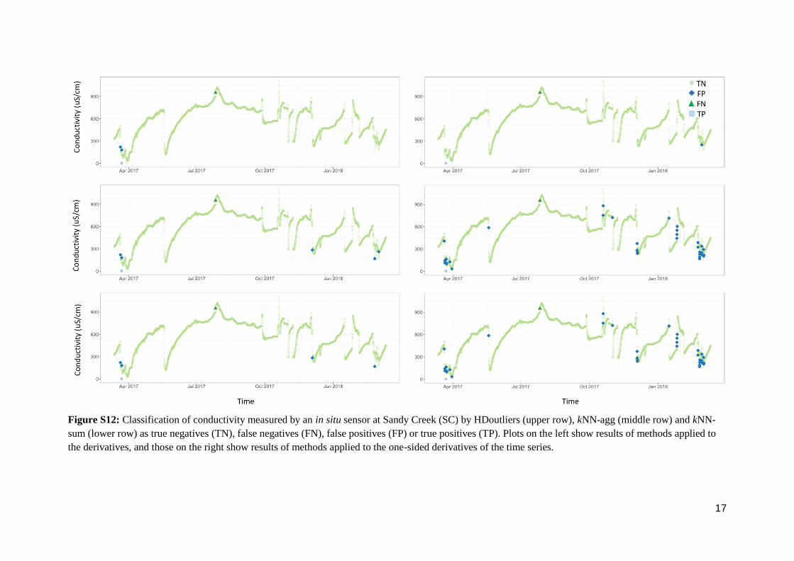
Figure S12: Classification of conductivity measured by an in situ sensor at Sandy Creek (SC) by HDoutliers (upper row), kNN-agg (middle row) and kNN-

sum (lower row) as true negatives (TN), false negatives (FN), false positives (FP) or true positives (TP). Plots on the left show results of methods applied to

the derivatives, and those on the right show results of methods applied to the one-sided derivatives of the time series.

18

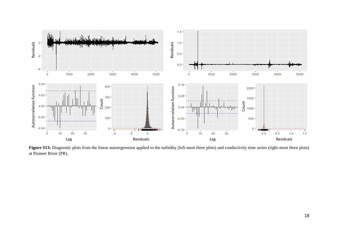
Figure S13: Diagnostic plots from the linear autoregression applied to the turbidity (left-most three plots) and conductivity time series (right-most three plots)

at Pioneer River (PR).

19

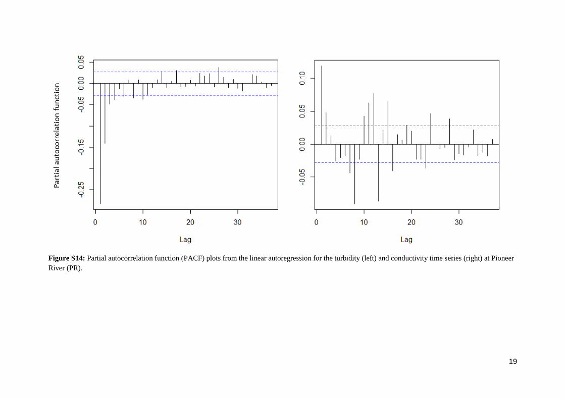
Figure S14: Partial autocorrelation function (PACF) plots from the linear autoregression for the turbidity (left) and conductivity time series (right) at Pioneer

River (PR).

20

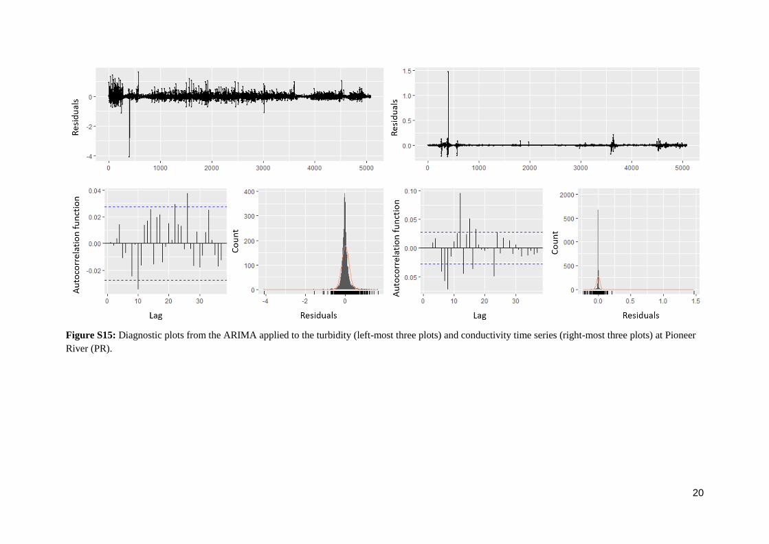
Figure S15: Diagnostic plots from the ARIMA applied to the turbidity (left-most three plots) and conductivity time series (right-most three plots) at Pioneer

River (PR).

21

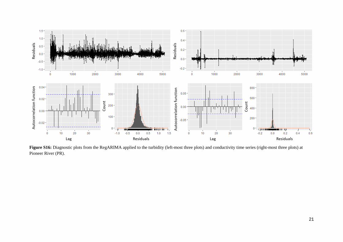
Figure S16: Diagnostic plots from the RegARIMA applied to the turbidity (left-most three plots) and conductivity time series (right-most three plots) at

Pioneer River (PR).

22

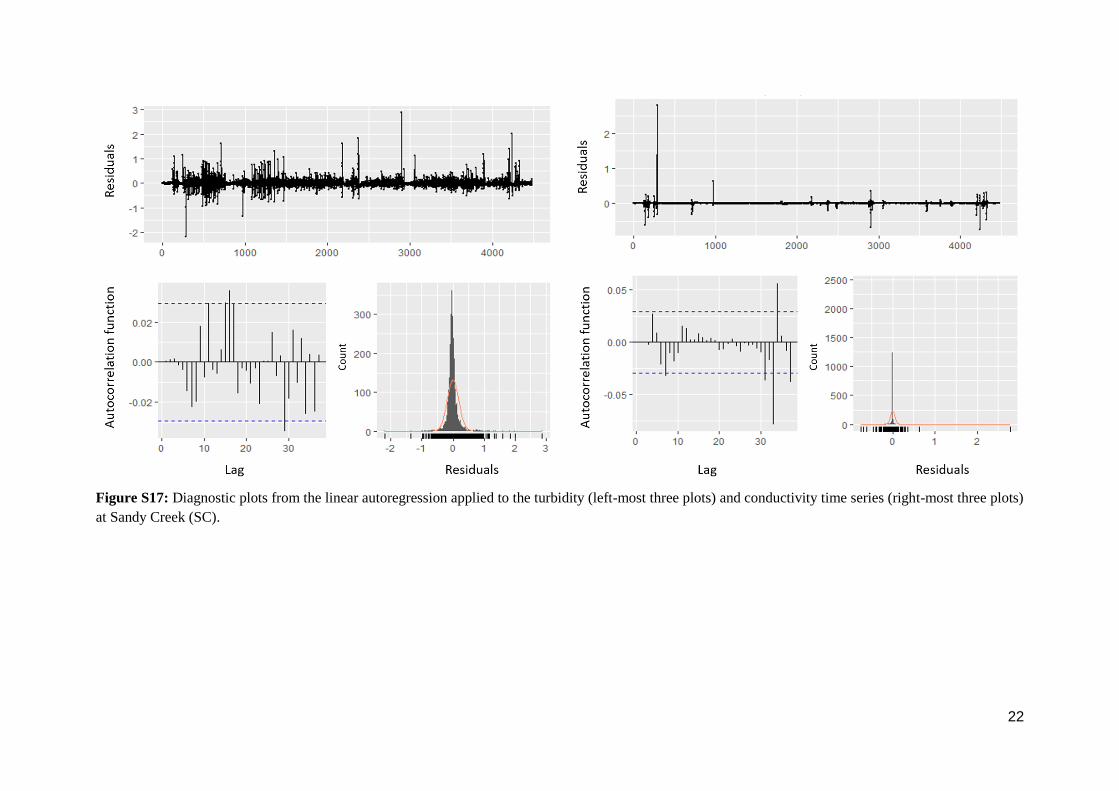
Figure S17: Diagnostic plots from the linear autoregression applied to the turbidity (left-most three plots) and conductivity time series (right-most three plots)

at Sandy Creek (SC).

23

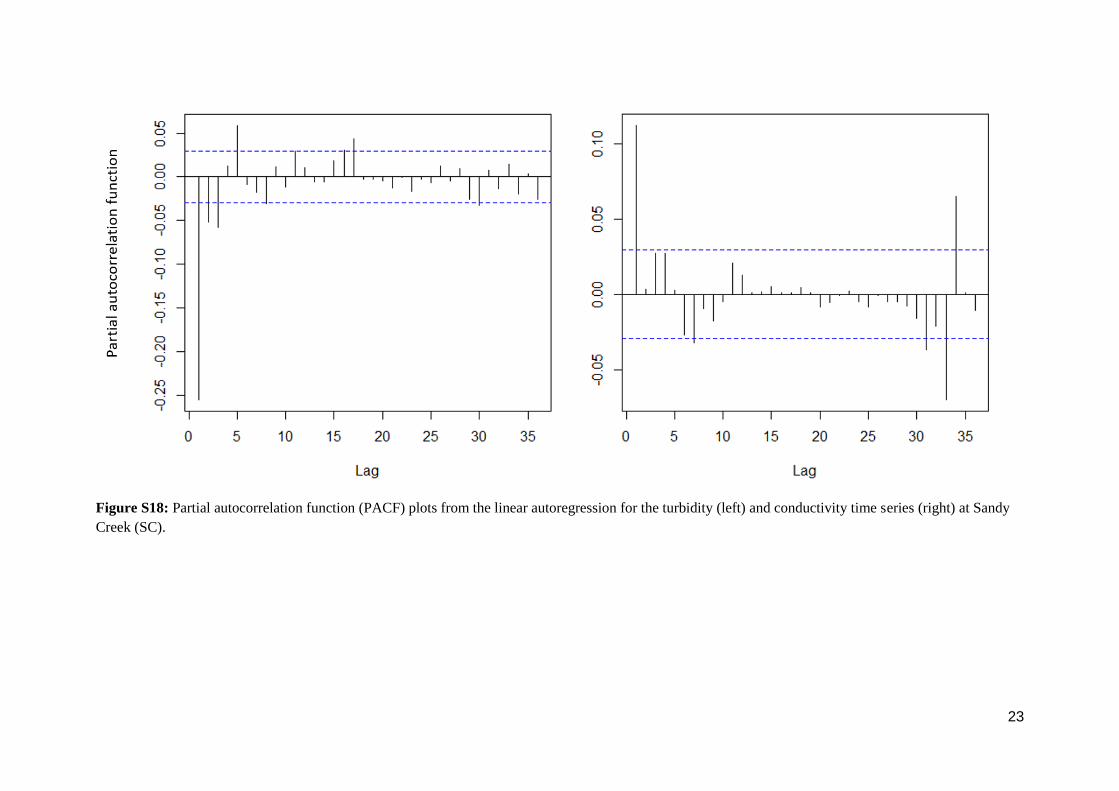
Figure S18: Partial autocorrelation function (PACF) plots from the linear autoregression for the turbidity (left) and conductivity time series (right) at Sandy

Creek (SC).

24

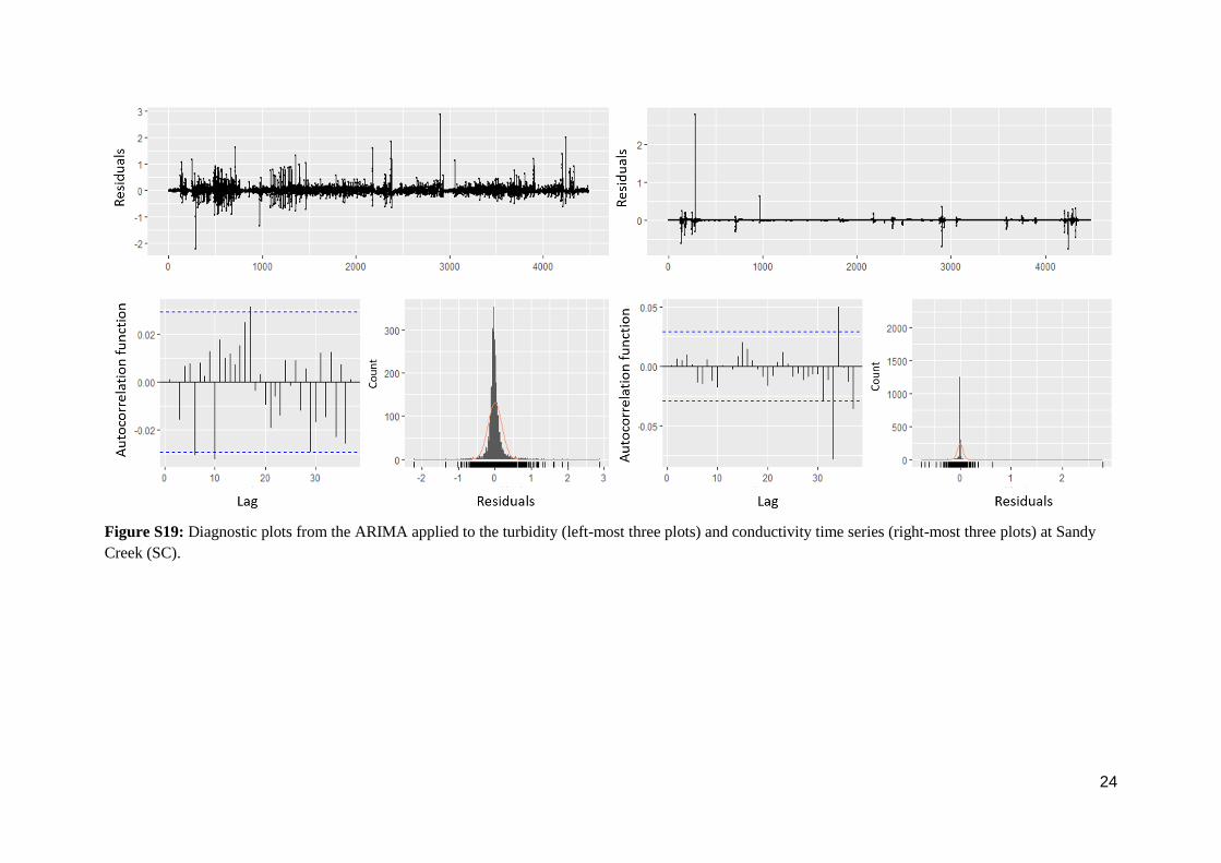
Figure S19: Diagnostic plots from the ARIMA applied to the turbidity (left-most three plots) and conductivity time series (right-most three plots) at Sandy

Creek (SC).

25

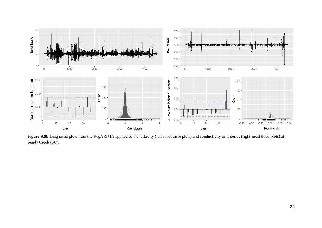
Figure S20: Diagnostic plots from the RegARIMA applied to the turbidity (left-most three plots) and conductivity time series (right-most three plots) at

Sandy Creek (SC).

26

References

Angiulli F. and Pizzuti C., Fast outlier detection in high dimensional spaces, In: European Conference on Principles of Data Mining and Knowledge

Discovery, 2002, Springer; Berlin, Heidelberg, 15–27.

Chan P.K. and Mahoney M.V., Modeling multiple time series for anomaly detection, In: Proceedings of the Fifth IEEE International Conference on Data

Mining, 2005, IEEE Computer Society; Washington, DC, USA, 90–97.

Fiebrich C.A., Morgan C.R., McCombs A.G., Hall P.K., Jr. and McPherson R.A., Quality assurance procedures for mesoscale meteorological data, J. Atmos.

Ocean. Technol. 27, 2010, 1565–1582.

Dereszynski E.W. and Dietterich T.G., Probabilistic models for anomaly detection in remote sensor data streams, In: Proceedings of the Twenty-third

Conference on Uncertainty in Artificial Intelligence, 2007, AUAI Press; Vancouver, BC, Canada, 75–82.

Hill D.J. and Minsker B.S., Anomaly detection in streaming environmental sensor data: a data-driven modeling approach, Environ. Model. Softw. 25, 2010,

1014–1022.

Hill D.J., Minsker B.S. and Amir E., Real-time Bayesian anomaly detection in streaming environmental data, Water Resour. Res. 45, 2009, W00D28.

Hossin M. and Sulaiman M.N., A review on evaluation metrics for data classification evaluations, Int. J. Data Min. Knowl. Manag. Process 5, 2015, 1–11.

Li J., Pedrycz W. and Jamal I., Multivariate time series anomaly detection: a framework of Hidden Markov Models, Appl. Soft Comput. 60, 2017, 229–240.

Madsen J.H., DDoutlier: Ddistance & density-based outlier detection. R package version 0.1.0, https://CRAN.R-project.org/package=DDoutlier, 2018.

Moatar F., Miquel J. and Poirel A., A quality-control method for physical and chemical monitoring data. Application to dissolved oxygen levels in the river

Loire (France), J. Hydrol. 252, 2001, 25–36.

Pang J., Liu D., Peng Y. and Peng X., Anomaly detection based on uncertainty fusion for univariate monitoring series, Measurement 95, 2017, 280–292.

Ranawana R. and Palade V., Optimized precision: a new measure for classifier performance evaluation, In: IEEE Congress on Evolutionary Computation,

2006, IEEE; Vancouver, BC, Canada, 2254–2261.

Sokolova M. and Lapalme G., A systematic analysis of performance measures for classification tasks, Inf. Process. Manag. 45, 2009, 427–437.

Talagala P., Hyndman R., Smith-Miles K., Kandanaarachchi S. and Munoz M., Anomaly Detection in Streaming Nonstationary Temporal Data. Working

Paper No. 4/18, 2018, Department of Econometrics and Business Statistics, Monash University.

Wilkinson L., Visualizing big data outliers through distributed aggregation, IEEE Trans. Vis. Comput. Graph. 24, 2018, 256–266.