A Framework for Component Based Software Architectures

by

K.M. van Hee, R.A. van der Toom, J. van der Woude and P.A.C Verkoulen

99--13

Eindhoven University of Technology Department of Mathematics and Computing Science

A Framework for Component Based Software Architectures

by

K.M. van Hee, R.A. van der Toom, J. van der Woude and P.A.C Verkoulen

ISSN 0926-4515

All rights reserved editors: prof.dr. J.C.M. Baeten

prof. dr. P.A.J. Hilbers

Reports are available at: http://www.win.tue.nVwin/cs

Computing Science Reports 99/13 Eindhoven, September 1999

99/13

A Framework for Component Based Software Architectures

K.M. van Heel, R.A. van def Toorn\ 1. van def Woude\ P.A.C. Verkoulen 1,2

'Eindhoven University of Technology, Department of Mathematics and Computing Science,

P.O. Box 513, NL-5600 MB, Eindhoven, The Netherlands {wsinhee, rvdtoom, japie, verkoulen}@win.tue.ni

20rigin DTS Infrastructure Solutions, P.O. Box 6435, NL-562l BA, Eindhoven, The Netherlands

peter. verkoulen@nl.origin-it.com

Abstract. A framework to design component based software architectures is presented. The framework incorporates concepts from workflow management and object orientation. The notation for defining architectures is based on the Unified Modelling Language. For semantics we use coloured Petri nets with time. Keywords: UML, Petri nets, software architecture, workflow nets, object-orientation, components

1 Introduction

In systems modelling there is a tendency to describe the essence of systems at higher levels of abstraction. The architecture of a system is such a high-level model. There are many modelling languages to describe systems at a high level of abstraction. These languages consist of a number of diagram techniques to describe a variety of views of a system. An example of such a language is the Unified Modeling Language [3]. A drawback of UML is that the views are not integrated. Therefore, UML does not guarantee that the views are consistent.

A way to prevent these problems is to use an executable model. If a model is executable, a computer can simulate the behaviour of the system; it is unambiguous and complete in the sense that all details to compute the behaviour of the system are defined. Executability of a model does not imply that it is a good description of the real system, however, the behaviour of the modelled system can be compared to the behaviour of the real system by running the executable model. It is an advantage if a language for executable models is based on a formal model, because then the semantics are well-defined and formal verification methods can be developed. There are several well-known modelling tools based on coloured Petri nets, for instance: ExSpect and Design ePN [4], [5]. These tools have no particular domain of application: they can be used to model all discrete dynamic systems. A consequence

of this is that they have no efficient notations for component based architectures that accommodate reuse of components.

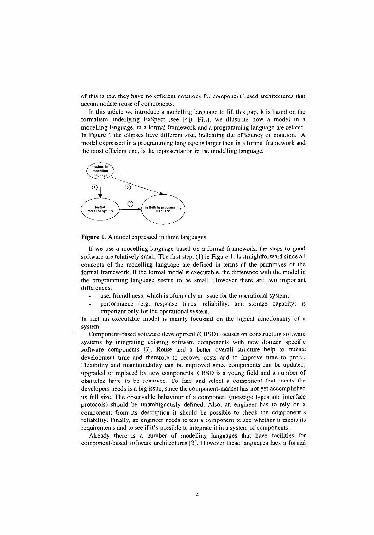
In this article we introduce a modelling language to fill this gap. It is based on the formalism underlying ExSpect (see [4]). First, we illustrate how a model in a modelling language, in a formal framework and a programming language are related. In Figure 1 the ellipses have different size, indicating the efficiency of notation. A model expressed in a programming language is larger then in a formal framework and the most efficient one, is the representation in the modelling language.

system in mDoeJJing language

CD

formal model 01 system

CD }-__ ~ system in programming language

Figure 1. A model expressed in three languages

If we use a modelling language based on a formal framework, the steps to good software are relatively small. The first step, (l) in Figure I, is straightforward since all concepts of the modelling language are defined in terms of the primitives of the formal framework. If the formal model is executable, the difference with the model in the programming language seems to be small. However there are two important differences:

user friendliness, which is often only an issue for the operational system; performance (e.g. response times, reliability, and storage capacity) is important only for the operational system.

In fact an executable model is mainly focussed on the logical functionality of a system.

'Component-based software development (CBSD) focuses on constructing software systems by integrating existing software components with new domain specific software components [7]. Reuse and a better overall structure help to reduce development time and therefore to recover costs and to improve time to profit. Flexibility and maintainability can be improved since components can be updated, upgraded or replaced by new components. CBSD is a young field and a number of obstacles have to be removed. To find and select a component that meets the developers needs is a big issue, since the component-market has not yet accomplished its full size. The observable behaviour of a component (message types and interface protocols) should be unambiguously defined. Also, an engineer has to rely on a component; from its description it should be possible to check the component's reliability. Finally, an engineer needs to test a component to see whether it meets its requirements and to see if it's possible to integrate it in a system of components.

Already there is a number of modelling languages that have facilities for component-based software architectures [3]. However these languages lack a formal

2

base. In terms of Figure 1 this implies that the formal model is missing. Therefore, analysis and simulation are not possible. In our framework for component based software architectures we provide concepts for executable system architectures in which:

components and their interactions with an environment are formally defined; the observable behaviour of components can be described and validated by simulation; components can be easily added, removed and replaced by other components.

The component framework we propose is based on coloured Petri nets with time [4, 5]. Timed coloured Petri nets have proven to be eligible for building compact models of complex systems. They have a formal semantics, a graphical notation, high expressiveness and there are many analysis techniques and software tools available. So, it is "proven technology" and is therefore a good start for a modelling language for CBSD. Petri nets are also applied to model workflow management systems, as described in [I]. This resulted in workflow nets (WF-nets).

In our framework, we will use WF-nets because they provide an excellent formalism to describe the dynamics of components, often referred to as transactions, protocols or object life cycles. We will also use the concept of object orientation [3] to describe data aspects of a system and to obtain a structure that integrates encapsulation, polymorphism and inheritance. Moreover, object oriented concepts are a pre-requisite for component technology; it gives the system the structure it requires to be 'componentised'.

2 Components as Petri Nets

Since Petri nets play an important role in defining the semantics of our notation, we summarise some elementary properties of Petri nets. For more details see [4], [5] and [6].

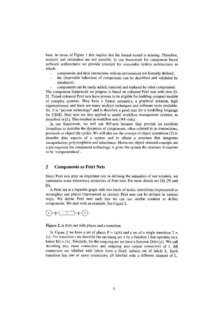
A Petri net is a bipartite graph with two kinds of nodes: transitions (represented as rectangles) and places (represented as circles). Petri nets can be defined in various ways. We define Petri nets such that we can use similar notation to define components. We start with an example. See Figure 2.

Figure 2. A Petri net with places and a transition.

In Figure 2 we have a set of places P = {a,b} and a set of a single transition T = {t}. For transition t we describe the incoming arc x by a function I that operates on t, hence I(t) = {x}. Similarly, for the outgoing arc we have a function O(t)={y}. We call incoming arcs input connectors and outgoing arcs output connectors of t. All connectors are labelled with labels from a fixed, infinite set of labels L. Each transition has one or more connectors, all labelled with a different element of L.

3

However, two transitions may usc the same connector labels. Note that the connectors x and yare attached to places. Places that are attached to input connectors are input places of a transition, likewise, output places are attached to output connectors. The function that matches (or glues) connectors to places is the function M. The function M operates on connectors for each transition separately, hence M(t,-) operates on the connectors of t. In Figure 2 we have M(t,x) = a and M(t,y) = b.

Definition 1. (Classical Petri net) A classical Petri net is a five tuple (P, T, I, 0, M) where (i) P is a finite set of places, (ii) T a finite set of transitions, (iii) I a function that assigns a set of input connectors to a transition, (iv) 0 a functiolL that assigns a set of output connectors to a transition and (v) M : T X L 1-7 P a match-junction that 'glues' for each transition the in- and

output connectors of the transition to places; M is a partial function that is only defined for connectors of transitions,

such that P and T are disjoint, for all transitions t the match function M(t,o) is defined for all connectors oft, V t E T: V x E I(t) u OCt): M(t,x) E P, V t E T: I(t) n OCt) = 0, each transition has at least one input connector.

In the places of a Petri net tokens may reside. The configuration of all tokens in a net is called the state of the net. If all input places of a transition have at least one token, the transition may fire, which means that the transition consumes from all its input places one token and that it produces for all its output places one token. (In fact it is a little more complicated: for each input connector a token is consumed and for each output connector one is produced and two or more connectors may be connected to the same place.) The firing of a transition determines a state-transition of the net. Given an initial state and a (finite or infinite) sequence of firings, we obtain a trace of the behaviour of the net.

In classical Petri nets, tokens are valueless and therefore transitions do not have logic. In coloured nets tokens have a value (traditionally called a "colour") and therefore transitions have "logic" to determine the values of the produced tokens as a function of the values of the consumed tokens. They also have "logic" to determine which tokens may be consumed and which tokens may not be consumed by a transition. This is called a pre-condition. It is a Boolean function on the input tokens. If the function value is "true", the transition may fire. Another feature is that in some output places no token need to be produced. In timed nets all tokens have a timestamp that is interpreted as the earliest moment the token might be consumed. The timestamp is computed in the transition that produces the token.

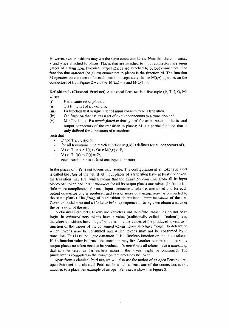
Apart from a classical Petri net, we will also use the notion of an open Petri net. An open Petri net is a classical Petri net in which at least one of the connectors is not attached to a place. An example of an open Petri net is shown in Figure 3.

4

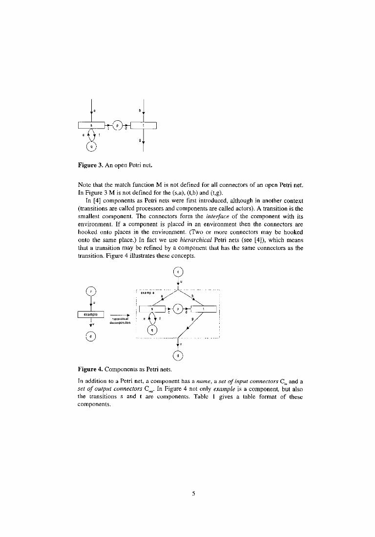
Figure 3. An open Petri net.

Note that the match function M is not defined for all connectors of an open Petri net. In Figure 3 M is not defined for the (s,a), (t,b) and (t,g).

In [4] components as Petri nets were first introduced, although in another context (transitions are called processors and components are called actors). A transition is the smallest component. The connectors form the interface of the component with its environment. If a component is placed in an environment then the connectors are hooked onto places in the environment. (Two or more connectors may be hooked onto the same place.) In fact we use hierarchical Petri nets (see [4]), which means that a transition may be refined by a component that has the same connectors as the transition. Figure 4 illustrates these concepts.

-hierarchical decomposilion

example

Figure 4. Components as Petri nets.

In addition to a Petri net, a component has a name, a set of input connectors Cin

and a set of output connectors C"". In Figure 4 not only example is a component, but also the transitions sand t are components. Table 1 gives a table format of these components.

5

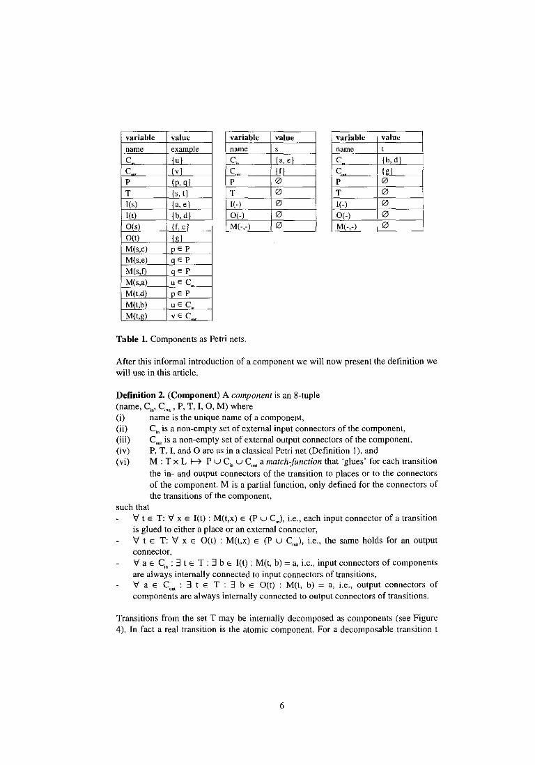
variable value variable value variable value

name example name s name t

C {u} C {a, e} C {b, d}

C {v I C {f} C {g} p {p,q} P 0 P 0

T {s, t} T 0 T 0 I(s) (a, e) l( -) 0 1(-) 0

I(t) {b,d} 0(-) 0 0(-) 0 O(s) (f, c I M(-,-) 0 M(-,-) 0 Oft) { g}

M(s,c) pE P

M(s,e) q E P

M(s,!) _ q E P

M(s,a) u E C M(t,d) pE P

M(t,b) uE C M(t,g) vEe

Table 1. Components as Petri nets.

After this informal introduction of a component we will now present the definition we will use in this article.

Definition 2, (Component) A component is an 8-tuple (name, C;n' COlli' P, T, I, 0, M) where (i) name is the unique name of a component, (ii) C;n is a non-empty set of external input connectors of the component, (iii) C'1ll1 is a non-empty set of external output connectors of the component, (iv) P, T, I, and 0 are as in a classical Petri net (Definition 1), and (vi) M : T X L H PuC;" u C,'"' a match-function that 'glues' for each transition

the in- and output connectors of the transition to places or to the connectors of the component. M is a partial function, only defined for the connectors of the transitions of the component,

such that V t E T: V x E I(t) : M(t,x) E (P u Cm)' i.e., each input connector of a transition is glued to either a place or an external connector, V t E T: V x E Oft) : M(t,x) E (P u C" .. ), i.e., the same holds for an output connector, V a E C;" : :3 t E T : :3 b E I(t) : M(t, b) = a, i.e., input connectors of components are always internally connected to input connectors of transitions, 'if a E C,,'" : :3 t E T : :I b E Oft) : M(t, b) = a, i.e., output connectors of components are always internally connected to output connectors of transitions.

Transitions from the set T may be internally decomposed as components (see Figure 4). In fact a real transition is the atomic component. For a decomposable transition t

6

we have that C;n := I(t) and C'~11 := OCt), and we call it an internal component, i.e., a component in a component. In this sense Definition 2 is recursive. If all internal components are atomic, i.e., transitions, and jf the sets C;n and C"U! are empty, then we have a Petri net as in Definition 1. (For a precise treatment of the transformation of hierarchical nets into classical nets we refer to [4].)

3 Structnred Components

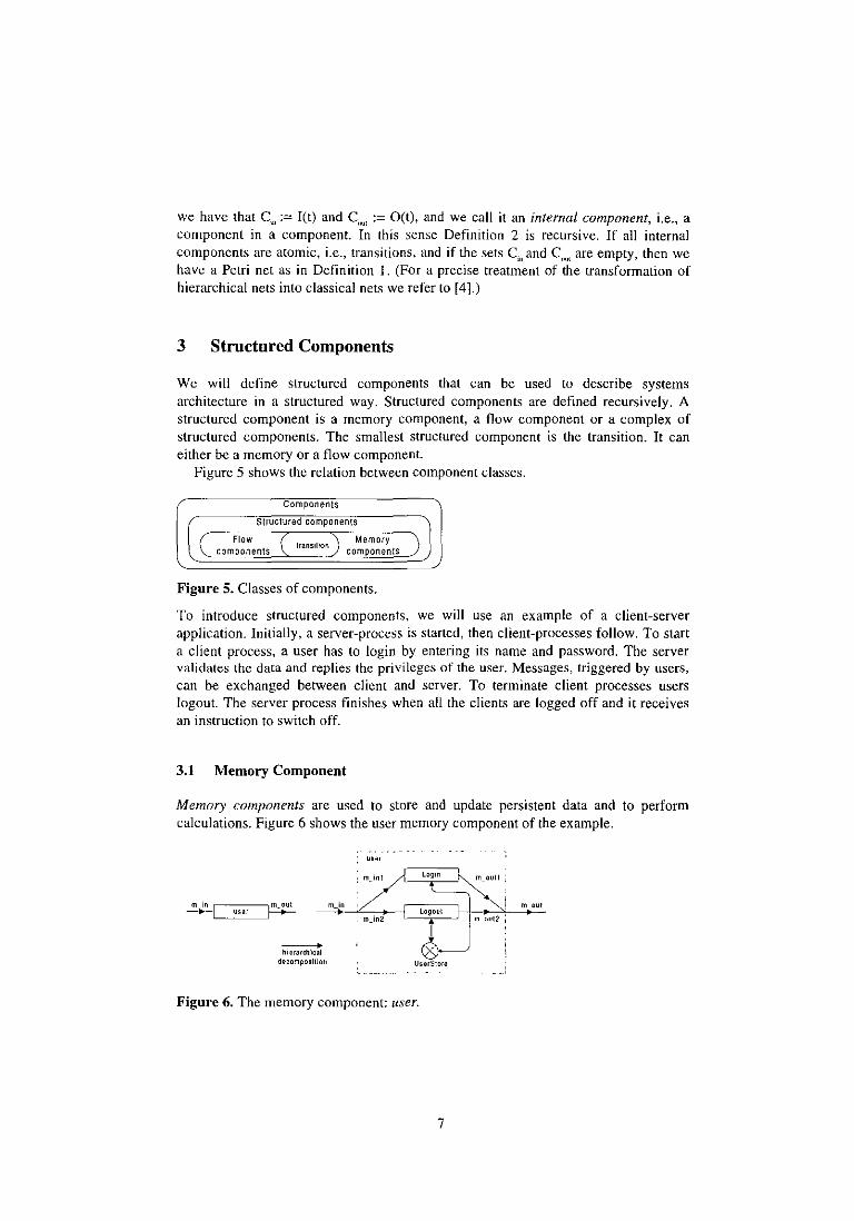
We will define structured components that can be used to describe systems architecture in a structured way. Structured components are defined recursively. A structured component is a memory component, a flow component or a complex of structured components. The smallest structured component is the transition. It can either be a memory or a flow component.

Figure 5 shows the relation between component classes.

Components

Structured components

( Flow ( components transition) co~ep~~~~ts )

Figure S. Classes of components.

To introduce structured components, we will use an example of a client-server application. Initially, a server-process is started, then client-processes follow. To start a client process, a user has to login by entering its name and password. The server validates the data and replies the privileges of the user. Messages, triggered by users, can be exchanged between client and server. To terminate client processes users logout. The server process finishes when all the clients are logged off and it receives an instruction to switch off.

3.1 Memory Component

Memory components are used to store and update persistent data and to perform calculations. Figure 6 shows the user memory component of the example.

~ user ~

---> hierarch"lcat

decomposition

USer

mJn2

Figure 6. The memory component: user.

7

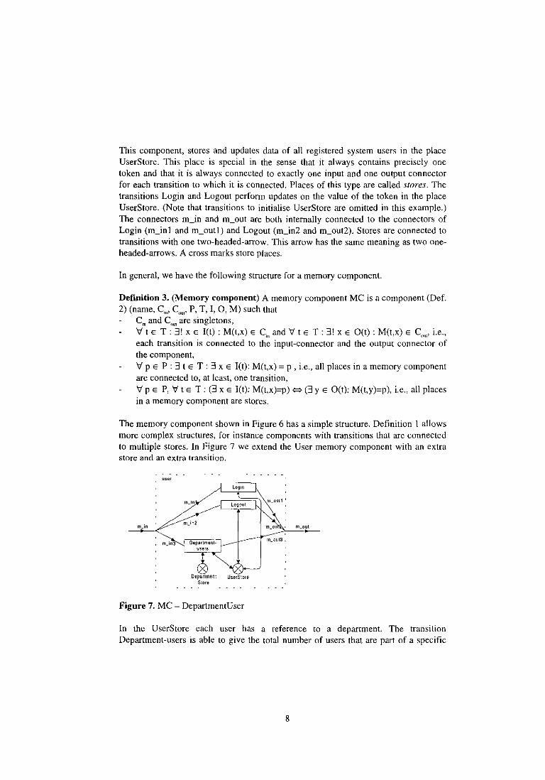
This component, stores and updates data of all registered system users in the place UserStore. This place is special in the sense that it always contains precisely one token and that it is always connected to exactly one input and one output connector for each transition to which it is connected. Places of this type are called stores. The transitions Login and Logout perform updates on the value of the token in the place UserStore. (Note that transitions to initialise UserStore are omitted in this example.) The connectors m_in and m_out are both internally connected to the connectors of Login (m_in! and m_outl) and Logout (m_in2 and m_out2). Stores are connected to transitions with one two-headed-arrow. This arrow has the same meaning as two one­headed-arrows. A cross marks store places.

In general, we have the following structure for a memory component.

Definition 3. (Memory component) A memory component Me is a component (Oef. 2) (name, C,,,, C,,.,, P, T, I, 0, M) such that

C in and C"III are singletons, V t E T : :I! x E I(t) : M(t,x) E C,,, and V t E T : :I! x E OCt) : M(t,x) E C""" i.e., each transition is connected to the input-connector and the output connector of the component, V PEP: :I t E T : :I x E I(t): M(t,x) = p , i.e., all places in a memory component are connected to, at least, one transition, V PEP, V t E T: (:I x E I(t): M(t,x)=p) <=> (:I y E OCt): M(t,y)=p), i.e., all places in a memory component are stores.

The memory component shown in Figure 6 has a simple structure. Definition I allows more complex structures, for instance components with transitions that are connected to mUltiple stores. In Figure 7 we extend the User memory component with an extra store and an extra transition.

user

mJn3

mJn2

Oepanment Slore

lIserStore

Figure 7. MC - DepartmentUser

In the UserStore each user has a reference to a department. The transition Department-users is able to give the total number of users that are part of a specific

8

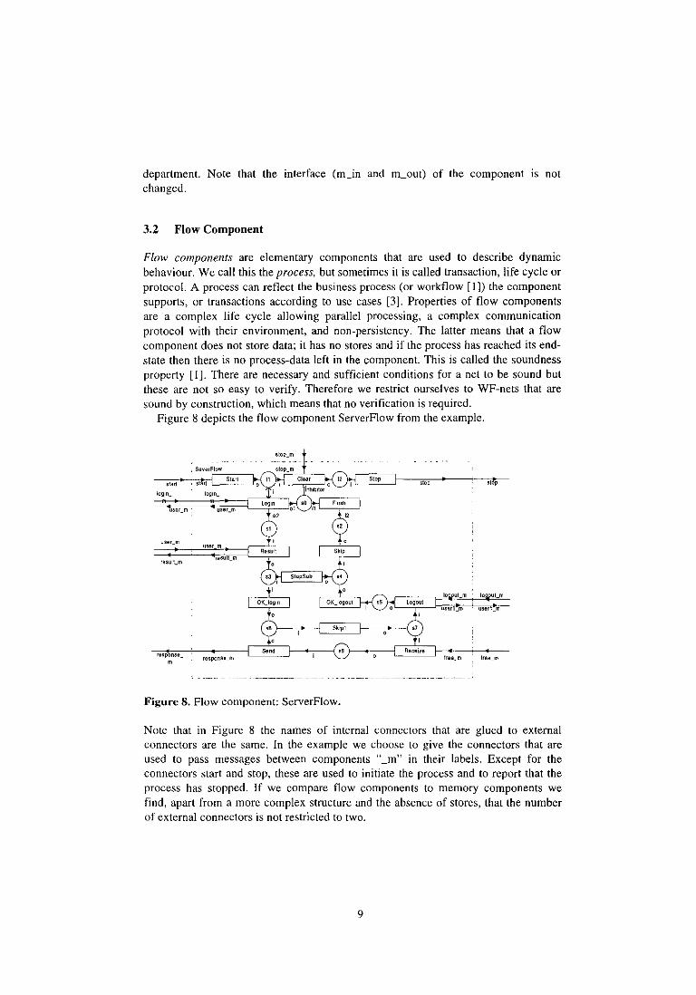
department. Note that the interface (m_in and m_out) of the component is not changed.

3.2 Flow Component

Flow components are elementary components that are used to describe dynamic behaviour. We call this the process, but sometimes it is called transaction, life cycle or protocol. A process can reflect the business process (or workflow [1]) the component supports, or transactions according to use cases [3]. Properties of flow components are a complex life cycle allowing parallel processing, a complex communication protocol with their environment, and non-persistency. The latter means that a flow component does not store data; it has no stores and if the process has reached its end­state then there is no process-data left in the component. This is called the soundness property [I]. There are necessary and sufficient conditions for a net to be sound but these are not so easy to verify. Therefore we restrict ourselves to WF-nets that are sound by construction, which means that no verification is required.

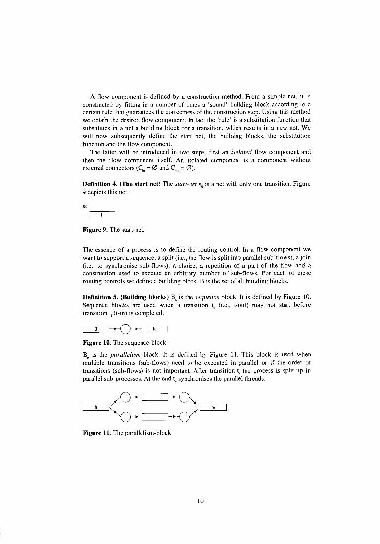
Figure 8 depicts the flow component ServerFlow from the example.

,"

Figure 8. Flow component: ServerFiow.

Note that in Figure 8 the names of internal connectors that are glued to external connectors are the same. In the example we choose to give the connectors that are used to pass messages between components "_m" in their labels. Except for the connectors start and stop, these are used to initiate the process and to report that the process has stopped. If we compare flow components to memory components we find, apart from a more complex structure and the absence of stores, that the number of external connectors is not restricted to two.

9

A flow component is defined by a construction method. From a simple net, it is constructed by fitting in a number of times a 'sound' building block according to a certain rule that guarantees the correctness of the construction step. Using this method we obtain the desired flow component. In fact the 'rule' is a substitution function that substitutes in a net a building block for a transition, which results in a new net. We will now subsequently define the start net, the building blocks, the substitution function and the flow component.

The latter will be introduced in two steps, first an isolated flow component and then the flow component itself. An isolated component is a component without external connectors (C,,, = 0 and C,,,,, = 0).

Definition 4. (The start net) The start-net So is a net with only one transition. Figure 9 depicts this net.

so:

Figure 9. The start-net.

The essence of a process is to define the routing control. In a flow component we want to support a sequence, a split (i.e., the flow is split into parallel sub-flows), ajoin (i.e., to synchronise sub-flows), a choice, a repetition of a part of the flow and a construction used to execute an arbitrary number of sub-flows. For each of these routing controls we define a building block. B is the set of all building blocks.

Definition 5. (Building blocks) B, is the sequence block. It is defined by Figure 10. Sequence blocks are used when a transition t" (i.e., t-out) may not start before transition t, (t-in) is completed.

Figure 10. The sequence-block.

B, is the parallelism block. It is defined by Figure II. This block is used when mUltiple transitions (sub-flows) need to be executed in parallel or if the order of transitions (sub-flows) is not important. After transition ti the process is split-up in parallel sub-processes. At the end t" synchronises the parallel threads.

Figure 11. The parallelism-block.

10

B)s the choice block, defined in Figure 12. It makes a choice between two or more transitions. Choices typically depend on token values or on incoming communication (triggers).

Figure 12. The choice·block.

Bj is the iteration block, defined in Figure 13. It is used to repeat a specific transition (or a number of transitions) a number of times until a specific condition becomes false (or some other event occurs).

Figure 13. The iteration·block.

FinaIly, we define block B,: the repeater block. It starts an arbitrary number of similar transitions or sub-flows simultaneously. A classical example where this kind of construction is applied is in handling an order for a customer (tlow) in which several order-lines (sub-flows) have to be processed. The repeater block is defined in Figure 14.

\; to

Figure 14. The repeater-block.

The repeater block requires explanation. It is a net in which the transition tj fires initially. Thereafter, a token in place p I may be consumed by transition tl or transition t2. Which of these transitions consumes the token depends on the token value or on tokens that are send to t 1 or t2 by communication connectors of t I and t2. These connectors are not visible in Figure 14. Suppose t2 fires. The token of p I is immediately placed back in pI. In p3 and p4 also tokens are produced. P4 is the input place of transition t4, which can be extended to a sub-flow. Now only t2 and t4 may fire. TI may not fire because the connection between tl and p3 is an inhibitor arc; this

II

means that tl may only fire if p3 is empty! Suppose t4 fires, then t3 is enabled. If t3 fires then place p3 is empty and tl and t" may subsequently fire to stop the flow. Note that as long as tl did not fire it is possible by t2 to start new sub-flows. All sub-flows need to end before the main flow can end.

The grey transitions in the repeater block are transitions that may not be replaced (see Def. 6) by other building blocks, replacement of these transitions would violate correct behaviour of the repeater block.

Note that: building blocks have precisely one start and one stop transition, denoted by t, and t", (This notation will be used in the definition of the substitution function.) building blocks are defined for the case n=2 (two parallel paths, two choices, one way there and one way back in a repetition). The construction method allows that the blocks are more generally defined for an arbitrary number of parallel paths, choices and repetitions, the inhibitor is only introduced in the net by block B,.

We now use the previous definitions to introduce the substitution-function. The

substitution function operates on an isolated component, therefore Cin = 0 and C"y\ =

121. We omit them in the following definition.

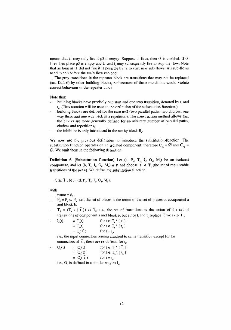
Definition 6, (Substitution function) Let (a, P" T" I" 0", M,l be an isolated component, and let (b, T", I", 0", M") E B and choose t E T" (the set of replaceable transitions of the net a). We define the substitution function

with name = d, P, = P, uP", i.e., the set of places is the union of the set of places of component a and block b, T, = (T" \ {t }) u T", i.e., the set of transitions is the union of the set of

transitions of component a and block b" but since t; and t" replace t we skip t , VI) = I.,(t) for t E T, \ { t }

= I"(t) for t E T" \ { t, } = I.n) for t = t"

i.e., the input connectors remain attached to same transition except for the

connectors of t , these are re-defined for tp

O,(t) = O,(t) for t E T, \ { t } = O"(t) for t E T" \ { t" } = 0,( t ) for t = t",

i.e., Od is defined in a similar way as 1,1'

12

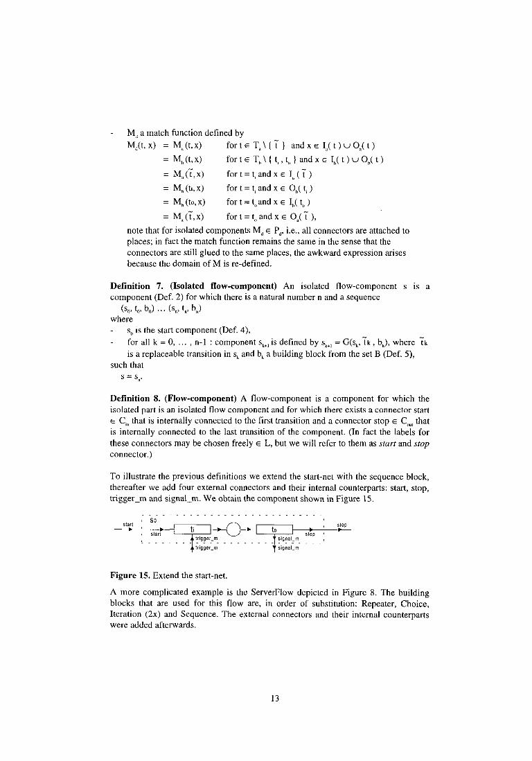
M" a match function defined by

M.,(t, x) = M" (t, x) for t E T" \ { t} and x E 1,,( t ) u OJ t )

= Mh(t,x)

= M,,(t,x)

M.(Ii,x)

M. (to, x)

= M"a,x)

for t E T. \ { t, ' t" } and x E 1.( t ) u 0.( t)

for t = t, and x E '" (I ) for t = t, and x E 0.( t, )

for t = t" and x E ,.( t" )

for t = t" and x E OJ t ), note that for isolated components Md E Pd' i.e., all connectors are attached to places; in fact the match function remains the same in the sense that the connectors are still glued to the same places. the awkward expression arises because the domain of M is re-defined.

Definition 7, (Isolated How-component) An isolated flow-component s IS a component (Def. 2) for which there is a natural number n and a sequence

(s()' tn' bo) ... (S", tn' bll)

where sf) is the start component (Def. 4),

for all k = 0, ... ,0-1 : component Sk+l is defined by Sk+l = G(Sk' tk, bk), where tk

is a replaceable transition in s, and b, a building block from the set B (Def. 5), such that

s = suo

Definition 8. (Flow-component) A t1ow-component is a component for which the isolated part is an isolated flow component and for which there exists a connector start E C jn that is internally connected to the first transition and a connector stop E C

OUl that

is internally connected to the last transition of the component. (In fact the labels for these connectors may be chosen freely E L, but we will refer to them as start and stop connector. )

To illustrate the previous definitions we extend the start-net with the sequence block, thereafter we add four external connectors and their internal counterparts: start, stop, trigger_m and signal_m. We obtain the component shown in Figure 15.

start So

start t;

trigger_m

trigger_m

Figure 15. Extend the start-net.

t. stop

slgnal_m

r signal_m

stop

A more complicated example is the ServerFlow depicted in Figure 8. The building blocks that are used for this t10w are, in order of substitution: Repeater, Choice, Iteration (2x) and Sequence. The external connectors and their internal counterparts were added afterwards.

13

Flow components are very close to WF-nets [IJ. Differences are that: flow components are components, they are open nets and not Petri nets; only nets that can be constructed by a graph grammar (building blocks) are allowed, there are constructions that can not be made with the graph grammar but that do exist in WF-nets; the repeater is a construction that is not allowed in WF-nets, because of the inhibitor arc; flow components have connectors to support communication between the flow component and its environment.

3.3 Structured Component

A structured component may encapsulate other structured components according to certain rules. To the environment, this new structured component defines an interface and inside the component the nested components are glued together by adding places between them. Components from the outside may not communicate directly with the nested components, but need to use the interface.

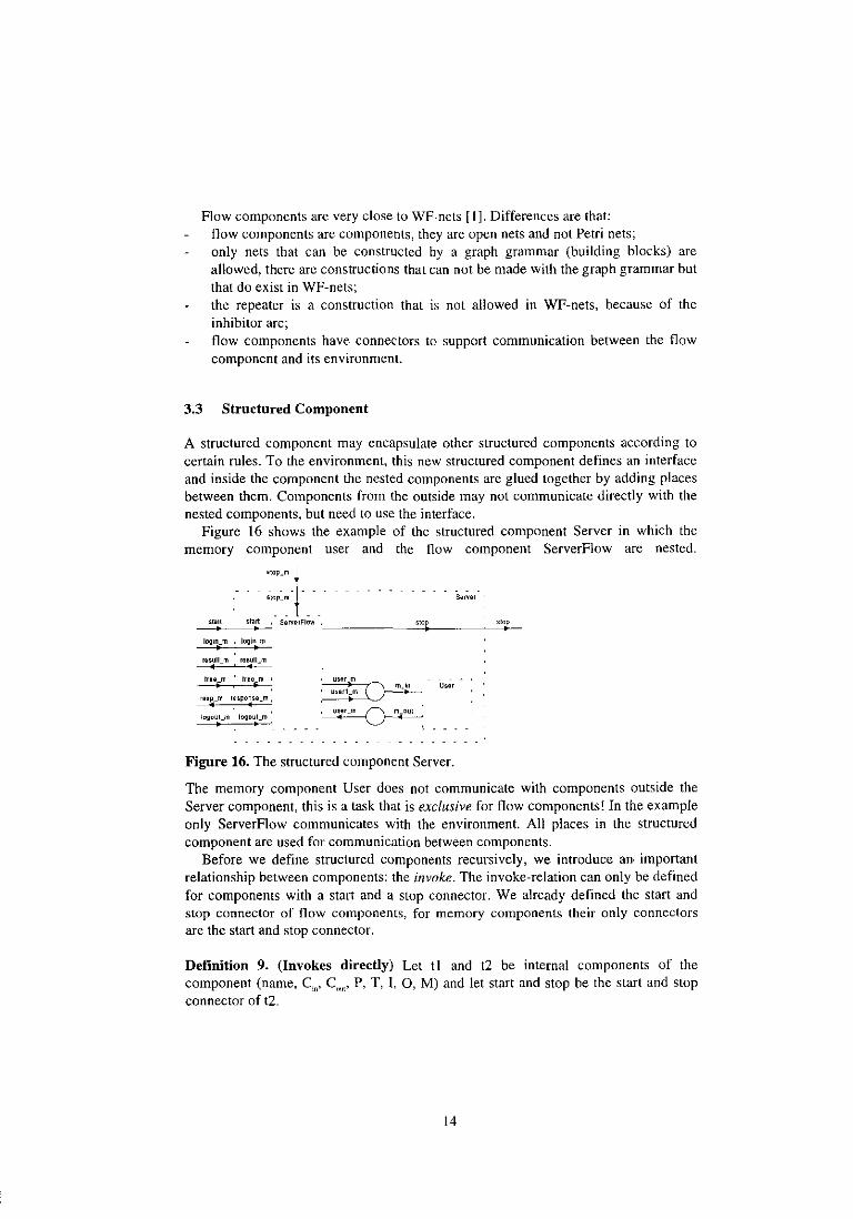
Figure 16 shows the example of the structured component Server in which the memory component user and the flow component ServerFlow are nested.

re5~" m ' m&~lcm '

Irum'lreem, If,

r&.~ m r~spo~S&_m,

logout m , logout_m I •

Usar

Figure 16. The structured component Server.

The memory component User does not communicate with components outside the Server component, this is a task that is exclusive for flow components! In the example only ServerFiow communicates with the environment. All places in the structured component are used for communication between components.

Before we define structured components recursively, we introduce an important relationship between components: the invoke. The invoke-relation can only be defined for components with a start and a stop connector. We already defined the start and stop connector of flow components, for memory components their only connectors are the start and stop connector.

Definition 9. (Invokes directly) Let tl and t2 be internal components of the component (name. C,", C"", P, T, I, 0, M) and let start and stop be the start and stop connector of t2.

14

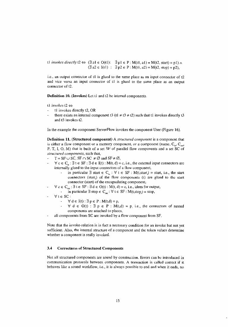
tl invokes directly t2 <=> (3 al E O(tl): (3a2E I(tl) :

:i pi E P: M(t!, al) = M(t2, start) = pi)" 3 p2 E P: M(t!, a2) = M(t2, stop) = p2),

i.e., an output connector of tl is glued to the same place as an input connector of t2 and vice versa an input connector of t1 is glued to the same place as an output connector of t2.

Definition 10. (Invokes) Let tI and t2 be internal components.

tI invokes t2 <=> tl invokes directly t2, OR there exists an internal component t3 (tl '" t3 '" t2) such that tI invokes directly t3 and t3 invokes t2.

In the example the component ServerFiow invokes the component User (Figure 16).

Definition 11. (Structured component) A structured component is a component that is either a flow component or a memory component, or a component (name, Cin • C

OUI'

P, T, I, 0, M) that is built of a set SF of parallel flow components and a set SC of structured components, such that,

T = SF uSC, SF n SC '" 0 and SF", 0, VeE C;, : 3 t E SF: 3 d E I(t) : M(t, d) = c, i.e., the external input connectors are internally glued to the input connectors of a flow component,

in particular 3 start E C;" : V t E SF : M(t,start,) = start, i.e., the start connectors (start[) of the flow components (t) are glued to the start connector (start) of the encapsulating component,

VeE C,., : 3 t E SF: 3 d E OCt) : M(t, d) = c, i.e., idem for output, in particular 3 stop E C,,"' : V t E SF: M(t,stop,) = stop,

V t E SC: V d E let) : 3 PEP: M(t,d) = p, V d E OCt) : 3 PEP : M(t,d) = p, i.e., the connectors of nested components are attached to places,

all components from SC are invoked by a flow component from SF.

Note that the invoke-relation is in fact a necessary condition for an invoke but not yet sufficient. Also, the internal structure of a component and the token values determine whether a component is really invoked.

3.4 Correctness of Structured Components

Not all structured components are sound by construction. Errors can be introduced in communication protocols between components. A transaction is called correct if it behaves like a sound workflow, i.e., it is always possible to end and when it ends, no

15

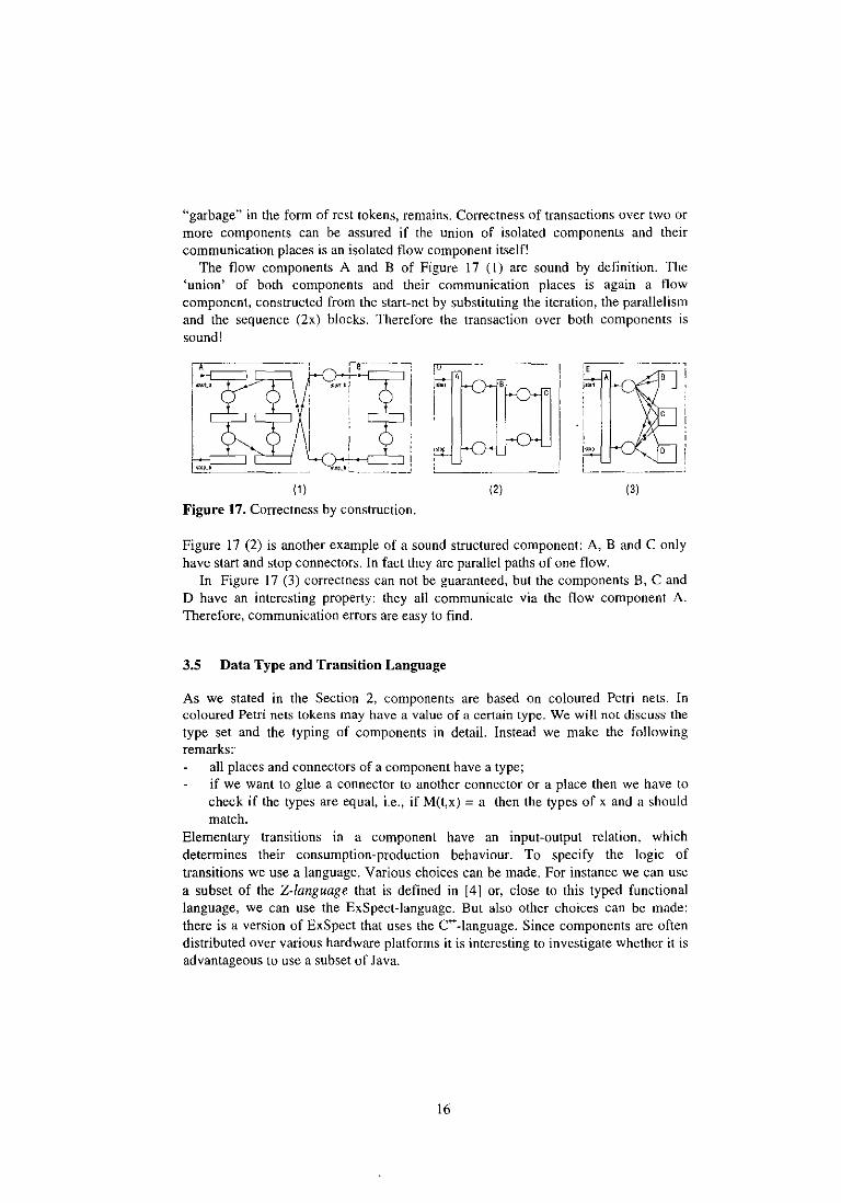
"garbage" in the form of rest tokens, remains. Correctness of transactions over two or more components can be assured if the union of isolated components and their communication places is an isolated tlow component itself!

The flow components A and B of Figure 17 (I) are sound by definition. The 'union' of both components and their communication places is again a flow component, constructed from the start-net by substituting the iteration, the parallelism and the sequence (2x) blocks. Therefore the transaction over both components is sound!

~,.---- -

(1) (2)

Figure 17. Correctness by construction.

I i

, !

! I"op

L~ _________ , (3)

Figure 17 (2) is another example of a sound structured component: A, Band Conly have start and stop connectors. In fact they are parallel paths of one flow.

In Figure 17 (3) correctness can not be guaranteed, but the components B, C and D have an interesting property: they all communicate via the flow component A. Therefore, communication errors are easy to find.

3.5 Data Type and Transition Language

As we stated in the Section 2, components are based on coloured Petri nets. In coloured Petri nets tokens may have a value of a certain type. We will not discuss the type set and the typing of components in detail. Instead we make the following remarks:

all places and connectors of a component have a type; if we want to glue a connector to another connector or a place then we have to check if the types are equal, i.e., if M(t,x) = a then the types of x and a should match.

Elementary transitions in a component have an input-output relation, which detennines their consumption-production behaviour. To specify the logic of transitions we use a language. Various choices can be made. For instance we can use a subset of the Z-language that is defined in [4] or, close to this typed functional language, we can use the ExSpect-language. But also other choices can be made: there is a version of ExSpect that uses the C++-language. Since components are often distributed over various hardware platforms it is interesting to investigate whether it is advantageous to use a subset of Java.

16

4 Classes and Objects

There is a relation between the static structure and the dynamic behaviour of components on one hand and classes [3] and objects on the other hand. We will discuss this analogy.

Flow components handle transactions or cases of a particular type. Therefore, all places of onc flow component are of the same type; we call it the flow type of the component. The flow component is considered as a class of this type. Each method of this class corresponds to a transition. Objects in this class are called flow objects. They refer to the transaction-data and are represented in the semantic model by a set of tokens of the same transaction (possibly more then one because of parallel paths). Note that flow objects have a life cycle and describe the dynamic structure of the component. They have a relatively short life and live exclusive in a flow component. If the flow reached its end state, they cease to exist.

Memory components operate on data objects (i.e., entities that have significance in the 'real' world, for instance customer data or invoices), on case data (i.e., the subject of a case, a case-owner, a date, decisions made) or on other persistent entities. A memory component offers the opportunity to access data of various types. Each store in the memory component may correspond to a different type and a transition may update multiple stores. Therefore, a memory component is more general than a class. A class method is only allowed to operate on objects of one type. A transition in a memory component corresponds to a method or a sequence of methods invoking each other, and so a memory component may represent more than one class. The objects of the classes are called memory objects. A set of memory objects of the same class is represented by a single token in a store. Memory objects have a relatively long life and live exclusively in memory components. They remain in a store even when the component is idle. In other words they are persistent. Memory object may have links to other objects in the same or different classes.

Communication places are used to connect components. They are attached to two transitions, one of each component: the first produces a token and second consumes a token. This corresponds to communication classes with a create- and a destroy­method only (no updates). The objects of this class are messages and are of the same type as the type of the place. Each message is represented by only one token. Messages have a very short life and they live exclusively between components. Flow or memory objects create them during a transaction.

5 Integrated Views and UML

Consistency of system views can be assured when they are based on an integrated model. This means that they can be derived by fixed rules or generated by running a simulation. From a structured component model we derive a number of views that are supported graphically by UML: the component view, the sequence diagram and the class diagram. Other views from UML such as activity diagrams and state diagrams are omitted because they are less general then coloured Petri nets.

17

5.1 The Component View

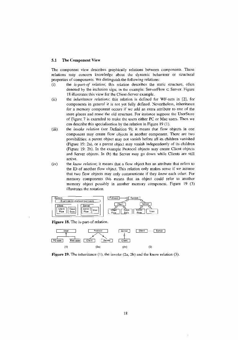
The component view describes graphically relations between components. These relations may concern knowledge about the dynamic behaviour or structural properties of components. We distinguish the following relations: (i) the is-port-oj relation; this relation describes the static structure, often

denoted by the inclusion sign; in the example: ServerFiow c Server. Figure 18 illustrates this view for the Client-Server example.

(ii) the inheritance relations; this relation is defined for WF-nets in [2], for components in general it is not yet fully defined. Nevertheless, inheritance for a memory component occurs if we add an extra attribute to one of the. store places and reuse the old structure. For instance suppose the UserS tore of figure.7 is extended to make the users either PC or Mac users. Then we can describe this specialisation by the relation in Figure 19 (I).

(iii) the invoke relation (see Definition 9); it means that flow objects in one component may create flow objects in another component. There are two possibilities: a parent object may not vanish before all its children vanished (Figure 19: 2a), or a parent object may vanish independently of its children (Figure 19: 2b). In the example Protocol objects may create Client objects and Server objects. In (b) the Server may go down while Clients are still active.

(iv) the know relation; it means that a tlow object has an attribute that refers to

the ID of another flow object. This relation only makes sense if we assume that two flow objects may only communicate if they know each other. For memory components this means that an object could refer to another memory object possihly in another memory component. Figure 19 (3) illustrates the notation.

System I Client server protocol (contract)

Figure 18, The is-part-of relation.

(1) (2,) (2b) (3)

Figure 19. The inheritance (1), the invoke (2a, 2b) and the know relation (3).

18

5.2 The Sequence Diagram

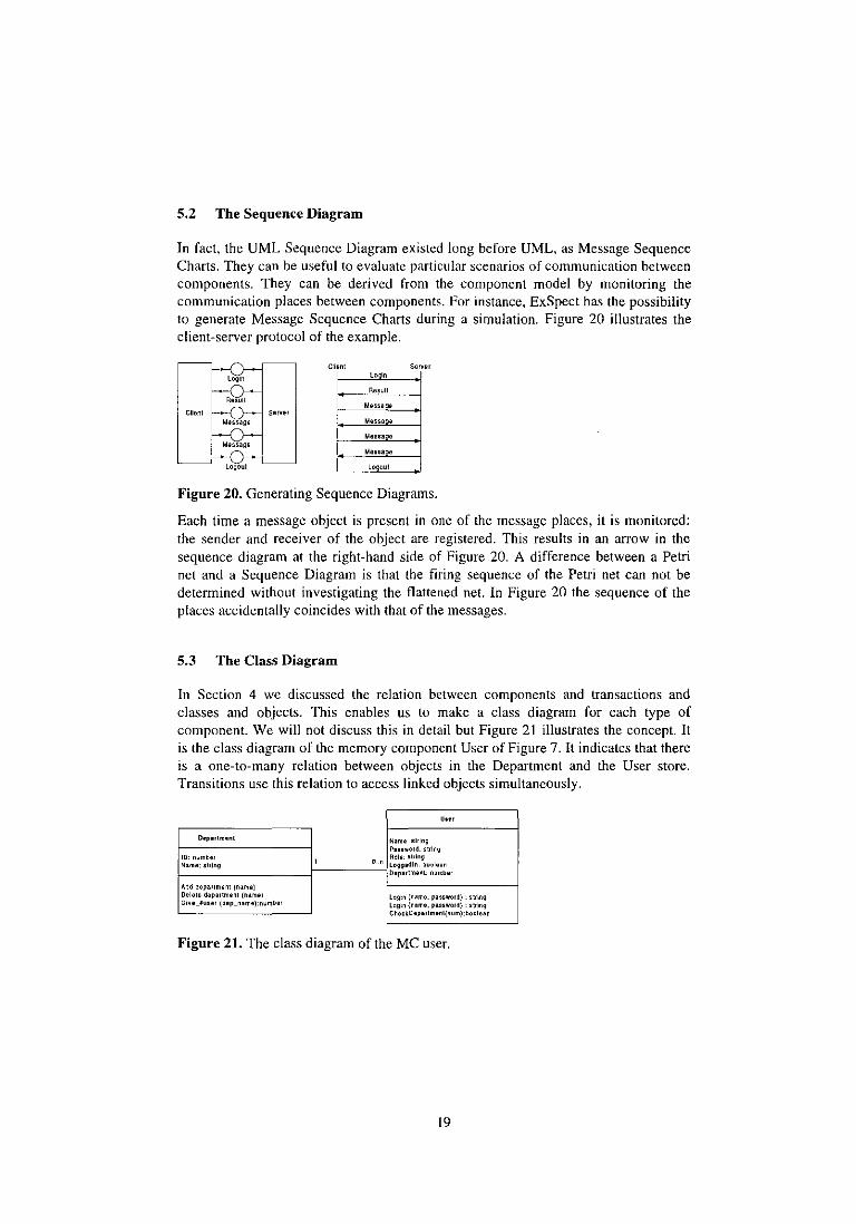
In fact, the UML Sequence Diagram existed long before UML. as Message Sequence Charts. They can be useful to evaluate particular scenarios of communication between components. They can be derived from the component model by monitoring the communication places between components. For instance, ExSpect has the possibility to generate Message Sequence Charts during a simulation. Figure 20 illustrates the client-server protocol of the example.

Client Sarve,

Login login

Result

Result Messa'l9

Client sorve' Massage Massa"

Messa e Massage

Menage

Logout Lo out

Figure 20. Generating Sequence Diagrams.

Each time a message object is present in one of the message places, it is monitored: the sender and receiver of the object arc registered. This results in an arrow in the sequence diagram at the right-hand side of Figure 20. A difference between a Petri net and a Sequence Diagram is that the firing sequence of the Petri net can not be determined without investigating the flattened net. In Figure 20 the sequence of the places accidentally coincides with that of the messages.

5.3 The Class Diagram

In Section 4 we discussed the relation between components and transactions and classes and objects. This enables us to make a class diagram for each type of component. We will not discuss this in detail but Figure 21 illustrates the concept. It is the class diagram of the memory component User of Figure 7. It indicates that there is a one-to-many relation between objects in the Department and the User store. Transitions use this relation to access linked objects simultaneously.

Uur

D'p.rlm.nl Nam. 'Iring Pa .. word: siring

I~.:::~m::"::':'~:::~~::~'~ _____ -I ____ "_ .. --jn ~;~~.~I:~~gboole'n t- Doparlmanl: O"rr.ber

Add dOpaJimOnl (namo) Delale depaJlrn.nl (nam"l Giv"_,u •• , (dop_n,mo):number

r--------1 Login (name. pas.word) Siring Login (namo. password) : 'Irlng ChockDopaJimOnl(num): bool •• n

Figure 21. The class diagram of the Me user.

19

6 Conclusions

In this paper we have demonstrated a way to describe components and the interaction between components in a formal way using coloured Petri nets. We distinguished three kinds of components namely flow components, memory components and structured components. Concepts from workflow management and object orientation are incorporated in these components and give them a well-founded structure. Together the components form a framework to describe and evaluate component­based (software) architectures. Important advantages of the framework are that it can be used to define system views formally and to extend inheritance concepts to components. In this way the framework forms a formal basis under (view) languages like UML. The tool ExSpect is suitable to develop and test structured componeots, but it does not support system views and correctness checks. It would be useful to extend ExSpect with these features.

References

I. W,M,P. van der Aalst. Verification of Workflow Nets. In P. Azoma and G. Balbo, editors, Proceedings of the International Conference on Information and Process Integration in Enterprises (I PIC '96), p. 179-201, 1996.

2. W.M.P. van der Aalst and T. Basten. Life Cycle Inheritance: A Petri-Net-Based Approach. In P. Azema and G. Balbo, editors, Proceedings of the 18th International Conference, on the Application and Theory of Petri Nets (ICATPN '97), Springer Verlag, Berlin, 1997.

3. G. Booch, J. Rumbaugh and I. Jacobson. The Unified Modeling Language User Guide. Addison Wesley, 1998.

4. K.M. van Hee. Information Systems Engineering: a Formal Approach. Cambridge University Press, 1994.

5. K. Jensen and G. Rozenberg, editors. High-level Petri Nets: Theory and Application. Springer-Verlag, New York, 1991.

6. W. Reisig, Petrinetze, eine Einflihrung. Springer-Verlag 1985 (2'· edition 1991). 7. C. Szyperski, Component Software: Beyond Object-Oriented Programming,

Addison Wesley, 1998.

20

Computing Science Reports

In this series appeared:

96101

96102

96/03

96105

96/06

96/07

96/08

96/09

96110

96/11

96112

96/13

96/14

96115

96117

96/18

96119

96120

96/21

96122

96/23

96124

96/25

97102

97/03

97/04

97/05

97/06

97/07

97/08

M. Voorhoeve and T. Basten

P. de Bra and A. Aerts

W.M.P. van dec Aalst

T. Basten and W.M.P. v.d. Aalst

W.M.P. van dec Aalst and T. Basten

M. Voorhoeve

A.T.M. Aerts, P,M.E. De Bra, J.T. de Munk

F. Oignum. H. Weigand, E. Verharen

R. B100, H. Geuvers

T. Laan

F. Kamareddine and T. Laan

T. Borghuis

S.H.J. Bos and M.A. Reniers

M.A. Reniers and J J. Vereijken

E. Boiten and P. Hoogendijk

P,D.V. van dec Stak

M.A Reniers

L. Feijs

L. Bijlsma and R. NederpeJt

M.e.A. van de Graaf and GJ. Houben

W.M.P. van dec Aalst

M. Voorhoeve and W. van dec Aalst

M. Vaccari and R.C. Backhouse

J. Hooman and O. v. Roosmalen

J. Blanco and A. v. Deursen

1.C.M. Baeten and l.A. Bergstea

J.C.M. Baeten and 1.J. Vereijken

M. Franssen

J.C.M. Baeten and l.A. Bergstra

P. Hoogendijk and R.C Backhouse

Department of Mathematics and Computing Science Eindhoven University of Technology

Process Algebra with Autonomous Actions, p. 12.

Multi-User Publishing in the Web: DreSS, A Document Repository Service Station, p.12

Parallel Computation of Reachable Dead States in a Free-choice Petri Net, p. 26.

A Process-Algebraic Approach to Life-Cycle Inheritance Inheritance = Encapsulation + Abstraction, p. 15.

Life-Cycle Inheritance A Petri-Nel-Based Approach. p. 18.

Structural Petri Net Equivalence, p. 16.

0008 Support for WWW Applications: Disclosing the internal structure of Hyperdocuments. p. 14.

A Fonnal Specification of Deadlines using Dynamic Deantic Logic, p. 18.

Explicit Substitution: on the Edge of Strong Normalisation, p. 13.

AUTOMATH and Pure Type Systems. p. 30.

A Correspondence between Nuprl and the Ramified Theory of Types, p. 12.

Priorean Tense Logics in Modal Pure Type Systems, p. 61

The /2 C·bus in Discrete-Time Process Algebra, p. 25.

Completeness in Discrete-Time Process Algebra, p. 139.

Nested collections and poiytypism, p. II.

Rea]-Time Distributed Concurrency Control Algorithms with mixed time constraints, p.71.

Static Semantics of Message Sequence Charts, p. 71

Algebraic Specification and Simulation of Lazy FunctionaJ Programs in a concurrent Environment, p. 27.

Predicate caJculus: concepts and misconceptions, p. 26.

Designing Effective Workflow Management Processes, p. 22.

StructuraJ Characterizations of sound workflow nets, p. 22.

Conservative Adaption of Workflow, p.22

Deriving a systolic regular language recognizer, p. 28

A Programming-Language Extension for Distributed ReaJ-Time Systems, p. 50.

Basic ConditionaJ Process Algebra. p. 20.

Discrete Time Process Algebra: Absolute Time, Relative Time and Parametric Time. p.26.

Discrete-Time Process Algebra with Empty Process, p. 51.

Tools for the Construction of Correct Programs: an Overview, p. 33.

Bounded Stacks, Bags and Queues. p. 15.

When do datatypes commute? p. 35.

97/09 Proceedings of the Second International Communication Modeling- The Language/Action Perspective, p. 147.

97110

97111

97/12

97/13

97114

97115

97116

97/17

97/18

98/01

98/02

98/03

98/04

98/05

98/06

Workshop on Communication Modeling, Veldhoven, The Netherlands, 9-10 June, 1997.

P.C.N. v. Gorp, E.J. Luit, D.K. Hammer E.H.L. Aarts

A. EngelS, S. Mauw and M.A. Reniers

D. Hauschildt, E. Verbeek and w. van der Aalst

W.M.P. van der Aalst

J.P. Groote, F. Monin and J. Springintveld

M. Franssen

W.M.P. van der Aals(

M. Vaccari and R.C. Bnckhouse

Werkgemeenschap Infonnatiewetenschap redactie: P.M.E. De Bra

W. Van der Aalst

M. Voorhoeve

J.CM. Baeten and J.A. Bergstra

RC. Backhouse

D. Dams

G. v.d. Bergen, A. Kaldewaij V.J. Dielissen

Distributed real-time systems: a survey of applications and a general design model, p. 31.

A Hierarchy of Communication Models for Message Sequence Charts, p. 30.

WOFLAN: A Petri-net-based Workflow Ana1yzer, p.30.

Exploring the Process Dimension of Workflow Management, p. 56.

A computer checked algebraic verification of a distributed summation algorithm, p. 28

AP-: A Pure Type System for First Order Loginc with Automated Theorem Proving, p.35.

On the verification of Inter-organizational workflows, p. 23

Calculating a Round-Robin Scheduler, p. 23.

lnfonnatiewetenschap 1997 Wetenschappelijke bijdragen aan de Vijfde Interdisciplinaire Conferentie Infonnatiewetenschap, p. 60.

Formalization and Verification of Event-driven Process Chains, p. 26.

State I Event Net Equivalence. p. 25

Deadlock Behaviour in Split and ST Bisimulation Semantics. p. 15.

Pair Algebras and Galois Connections, p. 14

Flat Fragments of CTL and CTL": Separating the Expressive and Distinguishing Powers. P. 22.

Maintenance of the Union of Intervals on a Line Revisited, p. to.

98/07 Proceedings of the workhop on Workflow Management: Net-based Concepts. Models. Techniques and Tools (WFM'98) June 22, 1998 Lisbon, Portugal edited by W. v.d. Aalst, p. 209

98/08 Informal proceedings of the Workshop on User Interfaces for Theorem Provers. Eindhoven University of Technology, 13-15 July 1998

edited by R.C. Backhouse, p. 180

98/09 K.M. van Hee and RA. Reijers An ana1yrical method for assessing business processes, p. 29.

98110 T. Basten and J. Hooman Process Algebra in PVS

98/11 J. Zwanenburg The Proof-assistemt Yarrow, p. 15

98112 Ninth ACM Conference on Hypertext and Hypermedia Hypertext '98

98113

98/14

99/01

99/02

99/03

99/04

Pittsburgh, USA, June 20-24, 1998 Proceedings ofthe second workshop on Adaptive Hypertext and Hypennedia.

J.F. Groote, F. Monin and J. v.d. Pol

T. Verhoeff (artikel voigt)

V. Bos and J.J.T. Kleijn

H.M.W. Verbeek, T. Basten and W.M.P. van der Aalst

R.C. Backhouse and P. Hoogendijk

S. Andova

Edited by P. Brusilovsky and P. De Bra, p. 95.

Checking verifications of protocols and distributed systems by computer. Extended version of a tutorial at CONCUR'98, p. 27.

Structured Operational Semantics of X , p. 27

Diagnosing Workflow Processes using Woflan. p. 44

Final Dialgebras: From Categories to Allegories, p. 26

Process Algebra with Interleaving Probabilistic Parallel Composition, p. 81

99/05

99/06

99/07

99/08

99/09

99110

99111

99112

M. Franssen, R.C. Veltkamp and W. Wesselink Efficient Evaluation of Triangular B-splines, p. I3

T. Basten and W. v.d. Arnst Inheritance ofWorkflows: An Approach to tackling problems related to change, p. 66

P. Brusilovsky and P. De 8m Second Workshop on Adaptive Systems and User Modeling on the World Wide Web, p. 119.

D. Bosnacki. S. Mauw, and T. Willemse Proceedings of the first intemationaJ syposium on Visual Fonnal Methods _ VFM'99

J. v.d. Pol, J. Hooman and E. de Jong Requirements Specification and Analysis of Command and Control Systems

T.A.C. Willemse The Ana1ysis of a Conveyor Belt System, a case study in Hybrid Systems and timed J1 CRL, p. 44.

J.C.M. Baeten and CA. Middelburg Process Algebra with Timing: Real Time and Discrete Time, p. 50.

S. Andova Process Algebra with Probabilistic Choice, p. 38.