A Framework for Identifying Accounting Characteristics for Asset

Pricing Models, with an Evaluation of Book-to-Price

Stephen H. Penman

Columbia Business School

shp38@columbia.edu

Francesco Reggiani

University of Zurich

francesco.reggiani@business.uzh.ch

Scott A. Richardson

London Business School

srichardson@london.edu

İrem Tuna

London Business School

ituna@london.edu

December, 2017

We are grateful to the Editor, Lu Zhang, and an anonymous referee for their helpful comments on prior drafts. We

thank Andrew Ang, David Ashton, Ray Ball, Stephen Brown, Jason Chen, Peter Christensen, Kent Daniel,

Francisco Gomes, Antti Ilmanen, Ralph Koijen, Matt Lyle, Patricia O’Brien, Jim Ohlson, Tapio Pekkala, Ruy

Ribeiro, Tjomme Rusticus, Kari Sigurdsson as well as seminar participants at Bristol University, London Business

School, Norges Bank Investment Management, Stockholm School of Economics, The University of Chicago Booth

School of Business, University of Waterloo, University of Technology Sydney, University of Zurich for helpful

discussions and comments. Earlier versions of the paper were under the title, “An Accounting-Based Characteristic

Model for Asset Pricing”. Francesco Reggiani acknowledges support from PwC Switzerland.

A Framework for Identifying Accounting Characteristics for Asset

Pricing Models, with an Evaluation of Book-to-Price

Abstract

We provide a framework for identifying accounting numbers that indicate risk and expected

return. Under specified accounting conditions for measuring earnings and book value, book-to-

price (B/P) indicates expected returns, providing justification for B/P in asset pricing models.

However, the framework also points to earnings-to-price (E/P) as a risk characteristic. Indeed,

E/P, rather than B/P, is the relevant characteristic when there is no expected earnings growth, but

the weight shifts to B/P with growth. Using this framework we resolve a puzzle: in contrast to

previous empirical research, we find that leverage is positively associated with future returns, as

predicted by theory.

Keywords: Book-to-price; earnings-to-price: growth and risk; accounting principles

JEL Classifications: G11 G12 M41

1

A Framework for Identifying Accounting Characteristics for Asset

Pricing Models, with an Evaluation of Book-to-Price

1. Introduction

A long stream of papers documents correlations between firm characteristics and future stock

returns. Empirical asset pricing research interprets some of these observed “characteristic”

correlations as evidence of a risk-return relationship and then proceeds to construct asset pricing

models with common risk factors based on the characteristics, as in Fama and French (1993).

Many of the characteristics involve accounting numbers, such as book-to-price, book rate-of-

return, and investment. However, these characteristics have largely been identified simply by

observing what predicts returns in the data, a data mining exercise that has resulted in a

proliferation of characteristics.1 A number of explanations for the phenomena have been offered,

although many of these are just conjectures. Presumably to emphasize the severity of the

problem, Novy-Marx (2014) finds that returns predicted by many of the observed characteristics

can be explained by sunspots, the conjunction of the planets, the temperature recorded at Central

Park Weather Station in Manhattan, and other seeming absurdities.

This paper presents a framework for identifying valid accounting characteristics for

asset pricing, yielding additional conditions for the identification beyond simply predicting

returns in the data. The framework develops from an expression that connects expected returns to

expectations of earnings and earnings growth, with the connection to risk determined by

accounting conditions. An identified characteristic is one that satisfies those conditions. The

ability to predict returns empirically then serves as validation.

We apply the framework to investigate book-to-price (B/P), identified in a “characteristic

regression model,” by Fama and French (1992) (FF) who then proceeded to construct an asset

pricing model in Fama and French (1993) that includes a book-to-price factor. That model stands

as perhaps the premier empirical asset pricing model, though subsequent research has expanded

1 In a survey of published papers and working papers, Harvey, Liu, and Zhu (2016) find 316 predictors, a number

they say likely under-represents the total. Green, Hand, and Zhang (2013 and 2014) find that, of 333 characteristics

that have been reported as predictors of stock returns, many predict returns incrementally to each other.

2

the set of characteristics to promote additional common factors, resulting in a proliferation of

factors (as well as characteristics).2 There is little theory for why B/P might indicate risk, though

conjectures abound.3 Our framework provides an explanation: under a specified accounting that

bears resemblance to GAAP, B/P forecasts expected earnings growth that the market deems to be

at risk. Our empirical analysis supports the predictions from our framework.

However, while the framework validates B/P in the FF model, it also points to earnings-

to-price (E/P) as a valid characteristic. Indeed, with no expected earnings growth, E/P alone

predicts the expected return and B/P is irrelevant. With growth, the weight shifts to B/P. The

paper also shows that the relative weights are related to firm size, another FF factor: for smaller

firms that typically have higher growth expectations, B/P is important for forecasting returns but,

for large firms with lower growth expectations, B/P is not important while E/P takes primacy.

Further, the paper shows how the relative weights on E/P and B/P depend on the accounting,

with the expected return under fair value accounting (where B/P = 1) given by E/P, but with the

weight shifting to B/P under historical cost accounting (where B/P is typically different from 1).

The paper also applies the framework to investigate the pricing of financing leverage risk

in the FF model. FF factors are said to incorporate financing risk, but there is no formal analysis

as to why. Indeed, Penman, Richardson, and Tuna (2007) show that the FF model does not price

financing leverage appropriately. Our framework separates the components of E/P and B/P that

pertain to operating risk from those that pertain to financing risk, with the expected returns

associated with each identified and reconciled to the expected equity return in accordance with

the Modigliani and Miller (1958) leveraging equation.

This separation enables us to revisit an issue long outstanding in empirical asset pricing:

While a basic tenet of modern finance, formalized in Modigliani and Miller (1958), states that,

for a given level of operating risk, expected equity returns are increasing in financial leverage,

2 Additional factors include momentum (Jegadeesh and Titman, 1993), investment (Liu, Whited, and Zhang, 2009

and Hou, Xue, and Zhang, 2015), profitability (Novy-Marx, 2012 and Fama and French, 2015), accruals quality

(Francis, LeFond, Olsson, and Schipper, 2005), among others.

3 Explanations for book-to-price include: (i) distress risk (Fama and French, 1992), (ii) the risk of “assets in place”

vs. “risk of growth options” (Berk, Green, and Naik, 1999; Zhang, 2005), (iii) low profitability (Fama and French,

1993), (iv) high profitability (Novy-Marx, 2012), (v) investment (Hou, Xue, and Zhang, 2015; Gomes, Kogan, and

Zhang, 2003; and Cooper, Gulen, and Schill, 2008) (vi) operating leverage (Carlson, Fisher, and Giammarino,

2004), and (vii) q-theory (Cochrane, 1991 and 1996 and Lin and Zhang, 2013).

3

research has had difficulty in documenting the positive relation. Indeed, papers largely report

negative returns to leverage.4 This is puzzling given how fundamental is the idea that leverage

requires a return premium. The failure to validate such a fundamental tenant of modern finance is

presumably due to a failure to identify and control for operating risk. By unlevering E/P and B/P

to capture operating risk, we are able to show that equity returns are increasing in leverage. This

not only yields an empirical documentation of the leverage effect that has escaped earlier

research, but also validates our framework: it identifies operating risk such that one observes that

leverage is appropriately priced. And it points to a deficiency in the FF model: both E/P and B/P

are relevant and, once that is recognized, leverage prices according to theory.

Our analysis maintains the standard assumption in asset pricing research that the market

prices risk efficiently. There is no imperative, of course, but we wish to address the research on

its own grounds.

2. The Framework: Connecting E/P and B/P to Expected Returns

The framework involves two key ideas. First, expected returns can be expressed in terms of

expected earnings and subsequent earnings growth, with that expected return determined by the

risk that these expected outcomes will not be realized. Second, given price, B/P and E/P are

accounting phenomena, so how they connect to risk and return depends on the accounting. With

the focus on B/P, the framework establishes conditions for the accounting for book value under

which B/P can (or cannot) indicate the risk of expected earnings and earnings growth not being

realized. Further, as book value and earnings articulate under accounting principles, the

accounting for book value also determines earnings, and thus E/P is also identified as a potential

risk characteristic.

We stress that the framework is not a formal model that connects accounting

characteristics to priced risk. That would require a generally accepted asset pricing model (that

identifies priced risk), and that we (collectively) do not have. While the general form is laid out

in no-arbitrage asset pricing theory in terms of common risk factors and sensitivities to those

factors, it is the identification of factors that has proved difficult. That, of course, is what the ad

4 See Bhandari (1988), Johnson (2004), Nielson (2006), George and Hwang (2010), Ipplolito, Steri and Tebaldi

(2011), and Caskey, Hughes and Liu (2012), for example. Penman, Richardson, and Tuna (2007) report the negative

relation with the FF model.

4

hoc empirical approach is trying to do—identifying characteristics from correlations with returns

in the data—and it is at this level that this paper operates. However, rather than identifying

characteristics simply by observed correlations with returns, the framework sets up additional

conditions to be satisfied. The empirical analysis then tests whether these conditions are indeed

satisfied.

We establish conditions under which (levered) E/P and B/P convey information about

expected levered returns and unlevered E/P and B/P convey information about expected

unlevered returns. Leverage then explains the difference between levered and unlevered expected

returns implied by these multiples consistent with no-arbitrage asset pricing theory. That sets up

our tests of whether leverage is priced empirically according to theory.

2.1 Expected Levered Returns

The data dredging approach to identification of characteristics targets forward stock returns. We

start by expressing these returns in terms of forecasted accounting outcomes via the clean surplus

accounting relation governing financial statements.5 This relation states that the book value of

common equity, B, increases with comprehensive income, Earnings, and decreases with the

distribution of net dividends to equity holders, d: Bt+1 = Bt + Earningst+1 - dt+1. The equation is

typically applied to substitute earnings and book values for dividends in the numerator of the so-

called residual income model (see Ohlson 1995, for example). But that research has nothing to

say about the denominator of the valuation model, the expected return at which the numerator is

discounted―the issue in this paper. Re-arranging the equation, dt+1 = Earningst+1 - (Bt+1 - Bt) and

substituting for net dividends in the stock return (with firm subscripts omitted), the expected

dollar return is explained by expected forward earnings and the expected change in the premium

of price over book value:

E(Pt+1+ dt+1 - Pt) = E[Earningst+1 + (Pt+1 - Bt+1) - (Pt - Bt)] (1)

(Expectations here and everywhere below are at time t when prices are formed.) Dividing

through by Pt to yield the expected one-year-ahead rate-of-return,

5 The formulation requires that clean-surplus accounting must apply only in expectation. Clean-surplus accounting

may be violated in accounting for earnings realizations, but expected deviations from clean-surplus must be mean

zero (as with the unrealized gains and losses on marketable securities that are recorded in comprehensive income

under GAAP and IFRS accounting).

5

))()(

()(

)()( 1111

11

t

tttt

t

tt

t

ttt

P

BPBPE

P

EarningsERE

P

PdPE

(1a)

The identity in equation (1) has long been recognized for realized returns, for example in Easton,

Harris, and Ohlson (1992). We adapt it here to apply to expected returns.6

If there is no expected change in the premium of price over book value, equation (1a)

shows that the expected rate-of-return is equal to the expected (forward) earnings yield.

However, given the earnings yield, a forecast of the expected return is completed with a (price-

denominated) forecast of the change in premium.

That, of course, requires an explanation of what induces a change in premium. First note

that payout does not affect premiums: dividends reduce book value, dollar-for-dollar, under the

clean-surplus accounting operation and also reduce price dollar-for-dollar under Miller and

Modigliani (1961) (M&M) conditions.7 Rather, an expected change in premium is induced by

expected earnings growth, as shown in Shroff (1995). If dividends do not affect the premium, the

expected change in premium due to the change in book value comes from earnings, by the clean-

surplus relation: E(Pt+1 – Bt+1) – (Pt – Bt) = E[(ΔPt+1 + dt+1 – (ΔBt+1 + dt+1)] for all E(dt+1) and,

with E(ΔPt+1 + dt+1) set by a no-arbitrage condition given Pt, the change in premium is

determined by E(ΔBt+1 + dt+1) = E(Earningst+1). Thus, for a given Pt, lower expected t+1earnings

implies an increase in the premium in t+1.8

6 Our focus is on the one-year-ahead expected return, the object of most of the research that predicts returns,

including our empirical work. However, at points below, the expected return is expressed as a constant over future

periods for simplicity, with the understanding that multi-period expected return is not necessarily the expected return

under an equilibrium asset pricing model (as often stated in interpreting bond yields). Our task is simply to identify

characteristics that might direct the construction of an asset pricing model, as in Fama and French (1992).

7 Dividends increase financing leverage and thus the expected return, but that is reflected in the E/P component of

the expected return which is increasing in leverage (see later). Some argue that, because of tax effects, price drops

by less than a dollar per dollar of dividends. Accordingly, we control for the dividend yield in the empirical analysis.

8 In other words, Pt is based on expected life-long earnings at time t so that, for a given price, the lower the earnings

expected for period t+1, the higher are earnings expected after t+1. That is expected earnings growth. This simply

reflects the workings of accrual accounting: accrual accounting allocates earnings to periods so, for total life-long

earnings expected in Pt, lower t+1 earnings means higher earnings in the future. The Internet Appendix

demonstrates.

6

However, while equation (1a) supplies a calculation for the expected return, it holds for

all accounting methods for allocating earnings to periods―even accounting that books earnings

to periods randomly; equation (1) is, after all, a tautology. The clean-surplus relation is not

sufficient; further specification is necessary for the accounting allocation to have implications for

risk and the corresponding expected return. That accounting must convey information about risk

that requires a discount to the current price, Pt, the denominator in equation (1a), to yield an

expected return commensurate with the risk. That is, the discount (in price) of expected life-long

earnings is conveyed by the allocation of those earnings to periods.

We consider four accounting cases. With a focus on B/P, we evaluate how B/P indicates

the expected return in each case, establishing conditions under which B/P bears no relation to the

expected return and conditions under which it does. The latter are the basis for our empirical

tests: are the conditions satisfied in the data? The four cases are demonstrated in the Internet

Appendix9. At all points, we assume that the market prices risk appropriately (market efficiency),

as is standard in asset pricing research.

2.1.1 Accounting where B/P has no Relation to the Expected Return

Mark-to-market accounting. If E(Pt+1 – Bt+1) = Pt – Bt = 0, the expected return equals the forward

earnings yield,t

t

P

EarningsE )( 1 , by equation (1a). The case is illustrated with a mark-to-market

bond. The expected one-period yield on a bond indicates its expected return and, under accrual

accounting, the effective interest method equates the expected earnings yield to the bond yield. A

bond cannot have earnings growth beyond that from a change in the effective amount borrowed,

but that is determined by the coupon rate, that is, payout. Thus, there is no expected change in

premium.

It follows that the FF model does not apply to mark-to-market bonds. Nor does it apply to

equities under mark-to-market accounting: B/P = 1 irrespective of the risk, so B/P cannot

indicate the expected return. However, the expected earnings yield indicates the expected return,

9 The Internet Appendix is available at the following link:

https://www0.gsb.columbia.edu/mygsb/faculty/research/pubfiles/25571/Appendix%20on%20Penman%2

0Web%20Page.pdf

7

yet the earnings yield does not appear in the FF model (while B/P inappropriately does). Case I

in the Internet Appendix demonstrates.

Permanent income accounting (no growth). For stocks, price usually differs from book value

because of historical cost accounting, so one looks to features of historical cost accounting that

induce a premium and thus potentially links B/P to expected returns. A benchmark case is that of

“permanent income” where earnings are recognized such that expected Earningst+1 is sufficient

for all future earnings: with full payout, E(Earningst+τ) = E(Earningst+1) for all τ such that there

is no expected earnings growth. Applying the clean-surplus relation with a constant expected

return, r, the expected premium for all t + τ is given by

).()1(

1).(

)1(

1)(

1

11

1

t

s

tsst

s

ststt BrEarningsEr

BrEarningsEr

BPE

.

Thus expected premiums are constant. Less than full payout results in earnings growth from

retention, but payout does not affect premiums. With no expected change in premium,

t

t

tP

EarningsERE

)()( 1

1

, by equation (1a).

As these conclusions hold for all Pt – B t, it follows that B/P does not indicate the

expected return in the no-growth case. Rather, the E/P ratio conveys the expected return, as in

the case of mark-to-market accounting. Case II in the Internet Appendix demonstrates.

Accounting with growth unrelated to risk and return. In the preceding accounting cases, B/P has

no relation to the expected return. It follows that B/P comes into play only with an expected

change in premium (and expected growth), and that is induced by reducing Earningst+1 and

increasing subsequent earnings (growth), that is, by Earningst+1 other than permanent earnings.

However, equation (1) is a tautology, so shifting earnings recognition from t+1 to the future has

no necessary effect on the left-hand side: the expected return is not affected, with no effect on

price, book value, or Bt/Pt. Case III in the Internet Appendix demonstrates.

2.1.2 Accounting where B/P indicates the Expected Return

The upshot of the accounting cases in section 2.1.1 is that B/P connects to risk only if the

accounting that induces growth (and a change in premium) conveys risk such that Pt is

8

discounted to yield a higher expected return (with the lower price yielding a higher Bt/Pt that

indicates that higher expected return).

To establish accounting conditions for this, we embrace the no-arbitrage Ohlson-Juettner

(2005) valuation model. Assume the form of the model that distinguishes expected short-term

growth from long-term growth:

A1. )1(

)1(1 2

1

r

g

rEarnings

P

t

t

where 11

122

t

tt

Earnings

rDividendsEarningsg > γ – 1 is the growth rate in expected earnings two

years ahead (with t+1dividends reinvested) and γ is (one plus) the growth rate in subsequent

expected abnormal earnings with the property that

t

t

Earnings

Earnings 1 → γ as τ → ∞; that is, γ is the

very long-run growth rate in expected earnings. (Here a subscript greater than t indicates an

expected value). Assume further a forecast of Earningt+2 given by

A2. tttt BEarningsGrDividendsEarnings 112 .

Thus,

1

2 1

t

t

Earnings

BGg (1b)

G can be interpreted as a persistence parameter for earnings, with book value adding to the

forecast through λ. Setting γ = 1,

r

Earnings

BG

rEarnings

P t

t

t

t 1

1

11

Therefore,

)1(1

1

t

t

t

t

Earnings

BG

P

Earningsr

9

t

t

t

t

P

B

P

EarningsG

1)1(

(1c)

The modeling suits our empirical endeavor, for it distinguishes growth in the short term,

g2, (for which one can observe realizations) from long-term growth (that is elusive empirically).

Further, γ is likely to be similar for all firms (in the long run), so g2 and r are the inputs that

discriminate in the cross-section.10 Equation (1c) sees r potentially related to both E/P and B/P,

but our focus at this point is on B/P. Assume further:

A3: λ > 0

The three assumptions yield two propositions which are the subject of our empirical tests:

P1. For a givent

t

P

Earnings 1 , the two-period-ahead earnings growth rate, g2 is increasing

in B/P.

P2. For a givent

t

P

Earnings 1 , r is increasing in B/P.

P1 follows from assumptions A2 and A3 under which g2 is increasing in11

1

ROEEarnings

B

t

t

in

equation (1b) and from the relation,t

t

t

t

t

t

P

Earnings

Earnings

B

P

B 1

1

. P2 follows directly from

equation (1c) and A3.11 Case IV in the Internet Appendix demonstrates.

The analysis is somewhat sterile without an appreciation of the accounting that induces

these properties and specifically λ > 0. Indeed, to predict a positive association between B/P and

earnings growth may come as quite a surprise, for it is commonly stated (without much

10 The analysis can be generalized for γ > 1with no effect on the directional relation between B/P and r. And it can

be generalized for B/P also forecasting γ.

11 Permanent earnings accounting is a special case. Setting λ = 0, r

t

t

P

EarningsG 1)1( which is satisfied for G

– 1 = r and rP

Earnings

t

t 1 , and B/P plays no role. (Earnings grow at the rate, r, because g2 refers to cum-

dividend earnings growth (with reinvested dividends); with full payout, there is no earning growth, as is section

2.1.1). As that holds for all B/P, it also covers the case of mark-to-market accounting, as in section 2.1.1.

10

documentation) that B/P is negatively associated with growth―a high P/B is a growth stock, not

a high B/P. The crucial condition in P1 is the negative relation between ROEt+1 and g2 (due to

assumed λ > 0).

Two features of historical cost accounting under GAAP suggest that accounting induces

this negative correlation, and these features connect the accounting to risk. First, the “realization

principle” that governs the allocation of earnings to periods states: under uncertainty, earnings

recognition is deferred to the future until the uncertainty has been resolved. Deferred earnings

imply higher expected earnings growth but also lower current earnings and ROE, ceteris paribus,

and the application of the principle under uncertainty ties the earnings deferral to risk. As an

empirical matter, Penman and Reggiani (2013) show that the deferral of earnings recognition is

priced in the stock market as if it indicates risk. Second, conservative accounting reduces ROE

by rapid expensing of growing investment, and correspondingly induces earnings growth

(Feltham and Ohlson 1995; Zhang 2000). The rapid expensing is applied when the outcome of

investments (in R&D and advertising, for example) are uncertain. Conservative accounting also

reduces book value, the denominator of ROE, but that serves to yield a higher ROE and lower

growth expectations when growth expectations are realized and uncertainty is (successfully)

resolved (and the forecast of g2 is reduced under A2). Thus, the lower B/P associated with the

high ROE indicates a lower expected return, in accordance with equation (1e).12

This is only suggestive, of course, and there is no necessity that the realization principle

and conservative accounting for risky investments are related to priced risk.13 That is the

empirical question that tests of P1 and P2 investigate.

12 While the conditions for B/P to indicate the expected return in equation (1c) are developed for a positive E/P,

GAAP accounting can produce negative E/P (and negative ROE), along with risky expected earnings growth―as

with negative earnings and ROE due to the expensing of R&D for a start-up firm where the gamble is on the R&D

investment paying off. We note that ROE and investment enter the Investment CAPM of Hou, Chen, and Zhang

(2015) and the extended Fama and French (2015) five-factor model, but with a different development from that here.

13 Modeling how GAAP accounting connects to priced risk is a challenging task. Ohlson (2008) lays out a model

where modified permanent income accounting produces earnings growth, with the growth rate set to equal the risk

premium (and P – B is increasing in the growth rate). However, the accounting does not mirror GAAP accounting.

Note that the framework here stands in contrast to a competing framework in Lyle, Callen, and Elliott (2013) and

Lyle and Wang (2015), for example, where the accounting is governed by an autoregressive process that also does

not represent GAAP; such a process models declining P – B (for P > B) rather than increasing P – B due to expected

earnings growth.

11

The analysis in this section is best viewed as that for a firm with no financing leverage,

for leverage changes the picture.

2.2 Expected Unlevered Returns

A core tenet of financial economics states that financial leverage adds to expected returns, yet

empirical research has had difficulty documenting a leverage risk premium in stock returns. In

this section we show that the accounting framework can be utilized to distinguish the expected

return due to operating risk from that due to financing. In contrast to most asset pricing models

where the leverage component is presumed to be subsumed by proposed factors (without much

explanation), the contribution of leverage to the expected return is explicit. That sets up the

empirical work to investigate whether leverage adds to average stock returns.

The analysis of unlevered returns recasts the balance sheet and income statement to

identify their unlevered components. In the balance sheet, B = NOA – ND where NOA (net

operating assets) denotes the unlevered book value (also called enterprise book value) and ND is

net debt. The clean surplus relation for the enterprise explains changes in NOA rather than

changes in B. The flows that explain the change are no longer Earnings and Net Dividends, but

rather Operating Income from the enterprise, OI, and Net Distributions to all claimants (the sum

of Net Dividends, d, and Net Distributions to Debt Holders, F), often referred to as Free Cash

Flow, FCF. NOA increase with operating income and decrease with net distributions to equity

and net debt holders. Thus, the clean surplus relation for the enterprise states that dt+1 + Ft+1 =

FCFt+1 = OIt+1 - (NOAt+1 - NOAt).

LetNOA

tP 1 be the price of the firm (enterprise price) and ND

tP 1 the price of the net debt. As

equity price,ND

t

NOA

tt PPP 111 , the dollar (levered) stock return can be expressed as:

)()()( 111111

ND

tt

ND

t

NOA

tt

NOA

tttt PFPEPFCFPEPdPE . (2)

That is, the (levered) equity return is the unlevered return after deducting the return to the net

debt holders. The first term on the right hand side is the expected dollar (unlevered) return.

Substituting the clean surplus relation for the unlevered firm and dividing through byNOA

tP yields

the expected unlevered (enterprise) rate of return,NOA

tR 1 :

12

NOA

t

t

NOA

tt

NOA

t

NOA

t

tNOA

tNOA

t

NOA

tt

NOA

t

P

NOAPNOAPE

P

OIERE

P

PFCFPE

)()()()()( 111

11

(2a)

This is the unlevered version of equation (1a); the expected unlevered return is expressed in

terms of the expected enterprise forward earnings yield, )( 1

NOA

t

t

P

OIE , and expected enterprise

earnings growth that produces an expected change in the premium of enterprise price, NOA

tP 1 –

NOAt+1.

It is clear that the same analysis that follows from equation (1a) to relate levered E/P and

B/P to expected (levered) returns also follows from equation (2a) to connect unlevered

(enterprise) E/P and B/P to unlevered returns. Indeed, the demonstrations in cases I – IV in the

Internet Appendix are demonstrations of unlevered relationships when there in zero financing

leverage. Note, in particular, that the conditions for B/P to indicate expected levered returns are

also those for the unlevered B/P to indicate expected unlevered returns.

2.3 Reconciling Levered and Unlevered Numbers and the Effects of Leverage

In this section we show that, just as levered and unlevered returns reconcile through leverage as

an implication of no-arbitrage, so do levered and unlevered E/P and B/P that potentially explain

those returns. From equation (2),

t

ND

tt

ND

t

t

NOA

tt

NOA

tt

P

PFPE

P

PFCFPERE

)()()( 1111

1

t

ND

tND

t

t

NOA

tNOA

tP

PRE

P

PRE )()( 11

)()()( 111

ND

t

NOA

t

t

ND

tNOA

t REREP

PRE , (3)

where )( 1

NOA

tRE is the expected unlevered return, )( 1

ND

tRE is the expected return for net debt, and

t

ND

t

P

Pis the amount of leverage. This, of course, is the Modigliani and Miller (1958) leverage

equation underlying the standard weighted average cost of capital calculation.

13

The same arithmetic reconciles the levered and unlevered earnings yields via financial

leverage. Recognizing that Earningst+1= OIt+1 – Net Interestt+1 (both after-tax) and making the

standard assumption that the book value of debt equals its market value (NDt =ND

tP ),

t

t

NOA

t

t

t

t

NOA

t

t

t

t

ND

InterestNetE

P

OIE

P

ND

P

OIE

P

EarningsE )()()()( 1111

(4)

where NOA

t

t

P

OIE )( 1 is the forward unlevered earnings yield and t

t

ND

InterestNet 1

is the firm’s borrowing

rate as reported in the financial statements. This expression is the accounting analog to the M&M

expected return equation (3). Financial leverage increases the levered E/P over enterprise E/P

provided that the unlevered (enterprise) earnings yield is greater than the borrowing rate.

Leverage is risky and adds to the expected return in equation (3), but leverage also adds to the

expected enterprise earnings yield in the same way, reinforcing the point that the expected

earnings yield is a basis for assessing risk and expected return. Leverage does not affect

premiums: 11111111 )( t

NOA

ttt

ND

t

NOA

ttt NOAPNDNOAPPBP if NDt =ND

tP . Thus, the

effect of leverage on the excepted levered return in equation (1a) is via the expected earnings

yield. Accordingly, without E/P in the model, FF model relies on B/P (or firm size or beta on the

market factor) to pick up leverage.

However, it is doubtful that B/P picks up leverage. Reconciling levered and unlevered

B/P, Penman, Richardson, and Tuna (2007) show that, if NDt =ND

tP ,

1

NOA

t

t

t

t

NOA

t

t

t

t

P

NOA

P

ND

P

NOA

P

B. (5)

Financial leverage, ND/P, increases (levered) B/P for an enterprise book-to-price greater than 1,

but reduces B/P for an enterprise book-to-price less than 1. Thus, if B/P indicates risk, it is

unlikely that it reflects both operating risk and leverage risk in a directionally consistent way.

Penman, Richardson, and Tuna (2007) indicate that it does not: for a sample of over 120,000 US

firm-years over the 1962-2001 period, that paper shows that while unlevered book-to-price is

robustly positively associated with equity returns, financial leverage is robustly negatively

associated with equity returns given the unlevered B/P. The results are robust to violations of the

14

NDt =ND

tP assumption. The negative relation between leverage and returns is strongest for the

group of firms where NOAP

NOA< 1. This is about 80 percent of firms and the firms where B/P is

decreasing in leverage, so the positive relation between B/P and returns in FF is not capturing

financial leverage. In short, both the B/P leveraging equation (5) and related empirical findings

indicate that B/P cannot handle differences in leverage risk in the cross-section.

Under Modigliani and Miller (1958) conditions, leverage does not affect price but adds to

the expected return by the M&M equation (3). By the same math that derives equation (4), it is

easy to show that leverage also adds to expected earnings growth:

InterestNet

t

OI

t

t

tOI

t

tt

ttEarnings

t ggEarnings

InterestNetg

InterestNetOI

InterestNetOIg 111

111

. (6)

Thus, the added expected return from leverage ties to higher expected earnings growth: while

leverage increases expected earnings growth in equation (6), the expected return also increases in

equation (3) to leave price unaffected. The connection of r to expected earnings growth (with

price unaffected) resonates with the propositions in the last subsection under which B/P is related

to r and g2. However, leverage reduces B/P in equation (5), except for the case where NOAP

NOA> 1,

andNOAP

NOAis typically less than 1. Thus, higher risk and growth associated with leverage typically

yields a lower, not higher, B/P.

This seeming conflict is explained by the modeling earlier. There, proposition P1 links

B/P to expected earnings growth, g2, via a negative relationship between B/P and ROEt+1 (for a

given E/P):t

t

tt P

Earnings

ROEP

B 1

1

1 1

. However, with the same math that derives equation (4),

t

tt

t

tt

tt

tt

t

tt

ND

InterestNetRNOA

B

NDRNOA

NDNOA

InterestNetOI

B

EarningsROE 1

11111

1 (7)

Thus, while leverage increases g2, it also increases ROEt+1, provided the unlevered book rate of

return,t

tt

NOA

OIRNOA 1

1

, is greater than the net borrowing rate. Accordingly, while leverage

15

increases r and g, it also increases ROEt+1, and an increase in ROEt+1 implies a lower B/P for a

given E/P. The leverage effect on ROEt+1 implies higher g2, thus the assumption in A2 that λ > 0

is violated.

Accordingly, in assessing the relationship of B/P to expected return, it is important to

differentiate the unlevered B/P from the leverage effect on (levered) B/P. This accords with

different accounting for (unlevered) operating activities versus that for financing activities.

Accounting that induces a positive relationship between B/P and r (by deferring earnings

recognition under uncertainty) is applied to operating activities under GAAP. However, debt is

approximately carried at market value. With approximate mark-to-market accounting, leverage

has no effect on the equity premium and the effect of leverage on the expected equity return is

captured by the E/P ratio. Case V in the Internet Appendix demonstrates.

2.4 Characteristic Regressions

To identify characteristics that indicate expected returns, empirical finance runs cross-sectional

“characteristic” regression models of forward stock returns on observed characteristics to

discover what characteristics predict stock returns. The Fama and French (1992) regression

model with beta, book-to-price, and size is an example. The preceding analysis imposes some

discipline on the specification of characteristic regressions, so this section lays out cross-

sectional regression models implied by that analysis.

The analysis points to E/P as well as B/P as indicators of the expected return. However,

the two are relevant under different accounting conditions, with B/P given weight only in the

case of expected earnings growth and where risk is related to that growth. Thus, with accounting

differing in the cross-section that presumably contains some no-growth firms, estimating a cross-

sectional model that applies to all firms is a doubtful exercise. However, we are interested in how

a cross-sectional model like that of FF would be modified by our analysis and what a typical

model would look like. Further, the earnings deferral accounting that justifies the inclusion of

B/P as a characteristic is pervasive across the cross-section that adheres to GAAP. So, we first

estimate a model that includes both E/P and B/P and then investigate conditions, implied by our

framework, where the weight shifts from B/P to E/P.

16

Under our analysis, E/P is identified and B/P explains returns for a given E/P under

specified conditions. Thus, our starting point is the following characteristic regression:

12

111

)(

t

t

t

t

tt

P

Bb

P

EarningsEbaR . (8)

A test for b1>0 is a test of the relevance of E/P. (We also include size and beta, also FF

characteristics, to ensure that they do not explain the omission of E/P in the FF model). The b2

coefficient is predicted to be positive if, given E/P, B/P indicates growth that is priced as risky.

With this starting point, we then investigate whether B/P is less important in explaining returns

(and E/P more important) in conditions where ex ante there is presumed to be less expected

earnings growth.

A characteristic unlevered return regression is similarly specified based on Equation (2a):

12

111

)(

tNOA

t

t

NOA

t

tNOA

tP

NOA

P

OIER , (9)

This is just a substitution of unlevered variables for the corresponding levered variables in

regression (8). Adding leverage to explain levered returns,

1321

11

)(

t

t

t

NOA

t

t

NOA

t

tt

P

ND

P

NOA

P

OIER (10)

Our framework predicts β3 > 0 if financial leverage adds to expected returns and if the included

operating variables are sufficient to control for operating risk.

However, the E/P and B/P leveraging equations (4) and (5) indicate that there is a “kink”

in the relation between leverage and returns for given unlevered E/P and B/P. For B/P, the kink

is at NOAP

NOA = 1. For E/P, the kink is at NOA

t

t

P

OIE )( 1 equal to the borrowing rate: when the unlevered

yield is less than the borrowing rate, E/P is decreasing in leverage. The Bank of America Merrill

Lynch BBB corporate bond index reports that the average effective yield for BBB rated

corporate issuers over the 1996 to 2011 period is about 6.5 percent. Thus, an after-tax borrowing

rate of about 4 percent (a before-tax rate of 6.5 percent with a 35 percent tax rate) implies that

the kink in equation (4) is at an unlevered E/P of 4 percent (and an unlevered P/E of 25).

17

Accordingly, our estimation of equation (10) is carried out for subsamples around these kinks.

Further, the M&M equation (3) indicates an interaction between operating risk and leverage, a

point stressed in Skogsvik, Skogsvik and Thorsell (2011) who note the importance of interaction

terms when assessing the relation between leverage and returns. Our empirical tests

accommodate this interaction.

The test for β3 > 0 serves to validate our characteristic identification framework. Prior

research has generally found a negative relation between leverage and equity returns, even after

controlling for conjectured operating risk characteristics.14 This negative relation can be

explained by leverage being negatively correlated with omitted operating risk factors. This is not

unreasonable if capital structure decisions are endogenous with respect to the perceived cost of

default and the after-tax benefits of debt financing. Indeed, theoretical models of capital

structure (Leland 1994) suggest that firms with higher levels of operating risk will endogenously

choose lower levels of leverage. Our framework suggests that operating risk can be identified

through the expected enterprise earnings yield and enterprise B/P. If so, we will have controlled

for operating risk, but only if the identified operating variables are sufficient to identify operating

risk. This qualification is important because additional omitted characteristics (with which

leverage is correlated) might indicate risky operating income growth.

We benchmark our regressions against an unlevered version of the FF characteristic

model:

1211 t

t

t

NOA

t

tt

P

ND

P

NOAR (11)

14 Bhandari (1988) finds a positive relation between monthly returns and leverage in annual cross-sectional

regressions over the years 1948-1966 but not from 1966-1979, and finds that most of the leverage effect is

concentrated in Januarys in years before 1966. Johnson (2004) finds a weak unconditional positive relation between

leverage and future returns but, after controlling for underlying firm characteristics (for example, volatility), the

relation between leverage and future returns becomes negative. George and Hwang (2010) document negative

returns to leverage, which they explain with a model of market frictions related to the costs of distress. Nielsen

(2006) finds negative returns to leverage after controlling for the three Fama and French factors and momentum, and

attributes the negative relation to correlated operating characteristics. Other attempts to identify correlated omitted

(operating) characteristics include Gomes and Schmid (2010) and Obreja (2013). Ippolito, Steri, and Tebaldi (2011)

and Caskey, Hughes, and Liu (2012) attribute the negative returns to deviations from optimal capital structure.

18

with an accommodation for the “kink” in the B/P leveraging equation (5). This equation unlevers

the B/P and adds leverage. Penman, Richardson, and Tuna (2007) report a negative coefficient

on leverage from this regression (with and without beta and size, the other two FF

characteristics) and thus conclude that the FF model does not price leverage appropriately.

Among their conjectures is the contention that the model does not deal with operating risk

appropriately (with which leverage may be negatively correlated). Our framework suggests that

the earnings yield is missing. Thus regression (11) serves as a benchmark to evaluate whether the

addition of the unlevered earnings yield in regression (10) turns the observed negative coefficient

on leverage to positive.

3. Data and Summary Statistics

Our analysis covers all U.S. listed firms on Compustat during the years 1962-2013 that also have

prices and monthly stock returns on CRSP. We exclude financial firms (with SIC codes 6000-

6999) because the separation of operating activities and financing activities is less clear for these

firms.

We require the following data items to be available for a firm-year to be included in our

analysis: book value of common equity (Compustat item CEQ), common shares outstanding

(CSHO), earnings before extraordinary items (IB), long-term debt (DLTT), and stock price at the

end of the fiscal year (PRCC). Other variables are set equal to zero if they are missing, but our

results are not particularly sensitive to this treatment. Firms with negative denominators in ratio

calculations (such as NOA

tP ) were deleted from the sample at any stage of the analysis that

required these numbers, as were firms with per-share prices less than 20 cents. Our results are

similar if we instead use a cut-off of $1.00 per-share. A total of 170,096 firm-year observations

are available for our analyses. For the regression analysis, we exclude firm-year observations

where any of the accounting ratios are in the top or bottom 2 percent of the distribution for the

relevant year. The number of firms available for the regression analysis each year ranges from

298 in 1962 to 5,287 in 1997, though that number varies depending on the regression

specification.

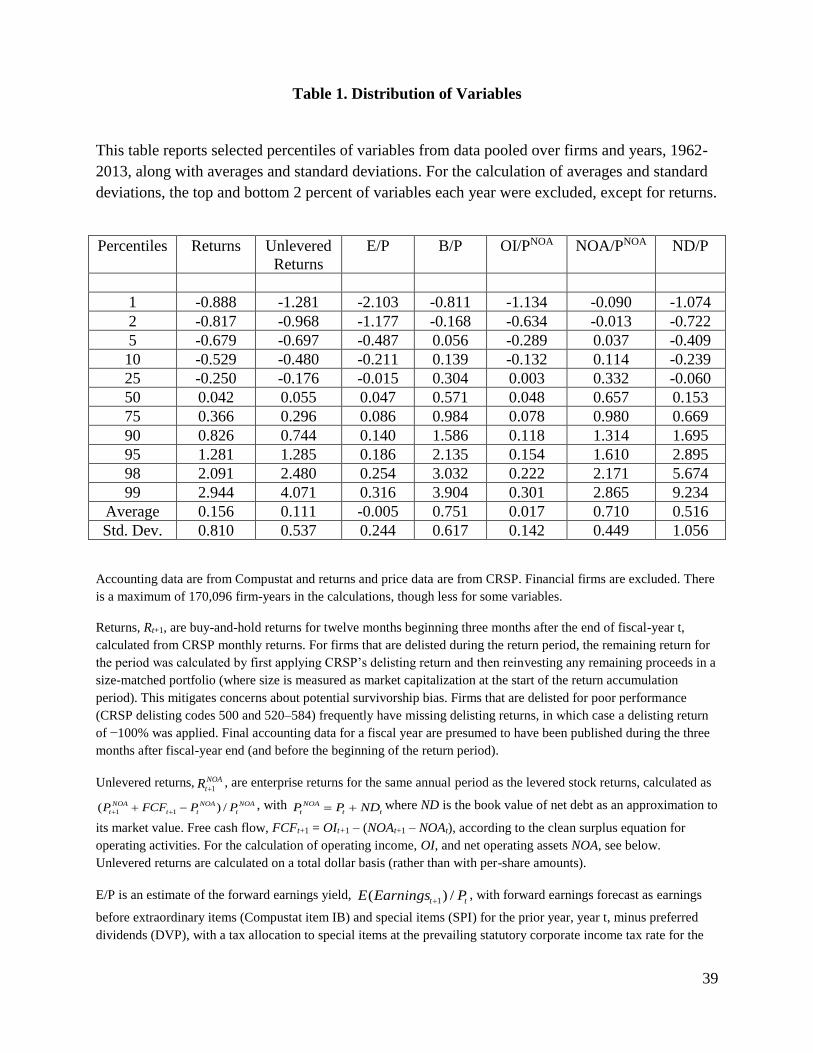
Table 1 summarizes the distribution of variables involved in the analysis. We report

percentiles for all of our primary variables based on the pooled set of data. Inferences are similar

19

when averaging percentiles from sorts each year. The notes to the table describe how each

variable was calculated, but a few additional comments are warranted. The regression

specifications require forecasts of forward earnings (for year t+1). We estimate forward earnings

to be the same as reported earnings for year t before extraordinary and special items. In support,

the average Spearman rank correlation between realized Earningst+1/Pt and Earningst/Pt is 0.672.

Using an estimate of forward earnings based on current (recurring) earnings not only enhances

the coverage to the full range of B/P ratios and firms sizes but also avoids (i) the problems of

(behavioral) biases and noise in analysts’ forecasts evidenced in Bradshaw, Richardson, and

Sloan (2001), Hughes, Liu, and Su (2008), and Wahlen and Wieland (2011), and (ii) the

challenge of “unlevering” earnings forecasts in a consistent manner across both analysts and

firms. The (market) leverage variable is calculated with the standard assumption that the market

value of debt,ND

tP , can be approximated by the book value of net debt, NDt. Penman,

Richardson, and Tuna (2007) find that estimates of Fama and French unlevered regressions are

robust with this approximation in the cases where there have been apparent changes in credit

worthiness that affect the market value.

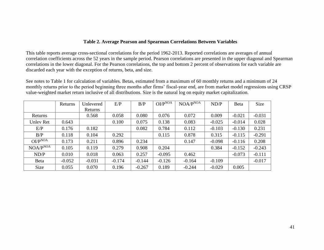
Table 2 reports average Pearson and Spearman cross-sectional correlations between the

variables in table 1, with beta and size added. In all cases, we calculate the pairwise correlation

each year and report averages of correlations across years. E/P and B/P are positively correlated

with both levered and unlevered equity returns for the following year, consistent with the

predictions from equation (1a). E/P and B/P are also correlated with each other (Spearman

correlation of 0.292). E/P and the unlevered earnings yield, OI/PNOA, are highly correlated

(Spearman correlation of 0.896), as are levered B/P and the unlevered B/P, NOAP

NOA, (Spearman

correlation of 0.908). Financial leverage, ND/P, has very little unconditional correlation with

either levered or unlevered returns, but ND/P is positively correlated with both the levered and

unlevered B/P ratios. Leverage is negatively correlated with the unlevered earnings yield. So the

failure of leverage to forecast returns may be due to its correlation with the operating earnings

yield, omitted in most tests in the literature, but appearing in regression equation (8).

4. E/P, B/P and Subsequent Earnings Growth

20

We first conduct tests of P1, a condition that is necessary for B/P to indicate expected returns in

our framework: for a given E/P, is B/P positively related to subsequent earnings growth?

4.1 B/P and Earnings Growth

First, we report the unconditional correlation between B/P and subsequent earnings growth.

Surprisingly, while it is often claimed that B/P is negatively related to growth, there is little

documentation of the relation.15 Panel A of table 3 reports average realized earnings growth

rates two years ahead, corresponding to g2, for ten portfolios formed from ranking firms on

levered B/P each year, and Panel B reports average realized operating income growth rates for

ten portfolios formed on enterprise (unlevered) book-to-price, NOAP

NOA, each year. The averages are

the mean of median growth rates for portfolios each year. These growth rates are those that an

investor would have experienced by investing in the respective portfolios.16 To accommodate

firms with negative earnings and a small earnings base, we compute growth rates by deflating

earnings changes with the absolute values of the level of earnings as described in the notes to

table 3.17 As growth in year t+2 is affected by investment in year t+1, both panels also report

growth rates in residual earnings to control for growth from added investment. In both cases,

residual earnings are calculated with a charge against beginning book value using the risk-free

rate for the relevant year.

15 Chan, Karceski, and Lakonishok (2003) report a weak positive correlation between B/P and earnings growth

when forming portfolios based on realized earnings growth over the next five and ten years. However, in their

regression analysis, they report no evidence of a relation between B/P and future earnings growth but a strong

negative association between B/P and future sales growth. Lakonishok, Shleifer, and Vishny (1994) report a positive

association between B/P and future earnings growth at least when comparing differences in geometric average

growth rates across the top and bottom decile of stocks formed on the basis of B/P. Finally, Chen, Petkova, and

Zhang (2008) and Chen (2017) report a positive association between B/P and subsequent dividend growth. The

mixed previous research on the unconditional relation between B/P and future earnings growth is not surprising as

Penman (1996) demonstrates that B/P can be associated with high growth, no growth, and negative growth.

Research has explored the relation between B/P and profitability (return on equity), for example in Penman (1992)

and Fama and French (1995) who document a negative correlation between the two in the cross-section, but

profitability is not to be confused with earnings growth.

16 The growth rates are not an estimate of expected earnings growth rates because

)(

)()(

1

2

1

2

t

t

t

t

EarningsE

EarningsE

Earnings

EarningsE . Rather, they are the average ex post growth outcomes experienced by investors.

17 The results are robust to calculations of earnings growth as total portfolio earnings in t+2 relative to that in t+1

and are similar when we require base earnings to be positive.

21

For both levered and unlevered B/P ratios, higher B/P is associated with higher growth. The

correlation between B/P and subsequent earnings growth at the individual firm level is low: an

average Spearman correlation of 0.052 and an average Pearson correlation of 0.047. (The

corresponding correlations for the unlevered numbers are 0.040 and 0.039.) Table 3 shows the

correlation is stronger at the portfolio level, with high B/P particularly associated with high

growth. The same pattern is seen in the residual earnings growth rates. Further analysis (not

reported) reveals that the positive relation between B/P and subsequent growth is primarily

associated with mid-cap and small firms; for large firms (the top third by market capitalization),

there is little correlation between portfolio B/P and growth. (We return to this issues in Table 6.)

Of course, growth two years ahead is only one year of the subsequent earnings growth that is

relevant for the determination of expected returns. However, survivorship issues overwhelm any

attempt to measure realized growth other than for the short term.18

4.2 B/P and Earnings Growth, Conditional on E/P

P1 refers to the conditional correlation of B/P with growth (that is, for a given E/P), rather than

the unconditional correlation. Panel A of table 4 reports mean realized growth rates for 25

portfolios formed by ranking firms first on enterprise earnings yield, OI/PNOA, and then, within

each OI/PNOA portfolio, on their enterprise book-to-price,NOAP

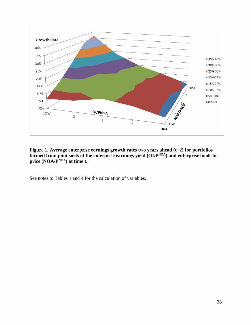
NOA.19 Figure 1 presents a graphical

depiction. Panel B reports average residual enterprise earnings growth rates These joint portfolio

sorts are performed each year; the table reports mean of portfolio median growth rates across

years. Enterprise earnings yield ranks growth negatively as expected; P/E ratios indicate growth.

But, for a given enterprise yield, higher NOAP

NOA is associated with higher subsequent growth on

average. Conditionally, unlevered B/P is a strong indicator of subsequent enterprise earnings

growth. P1 is confirmed. Further analysis (not reported) partitioned firms by market

18 For this table and that for Panel A in Table 4, we repeated the analysis for years t+3 – t+5 ahead with similar

results, albeit presumably with more survivorship bias.

19 Penman and Reggiani (2013) report a similar matrix of portfolios, constructed by dividing the total future levered

earnings expected in price into short-term and long-term components, and show that those portfolios are actually

equivalent to portfolios from a joint sort on E/P and B/P (as here). Long-term earnings relative to short-term

earnings is earnings growth, so the Penman and Reggiani (2013) results underscore our framework where the

expected returns are increasing in expected earnings growth if that expectation is at risk.

22

capitalization and found that, for large firms, portfolio OI/PNOA and subsequent growth are

positively related, but there is little correlation between NOAP

NOA and growth within OI/PNOA

portfolios, expect in the lowest E/P portfolio; the conditional correlation between NOAP

NOA and

subsequent growth is associated primarily with mid-cap and small firms. (Table 6, later, comes

back to this point.)

Panels A and B show that the relationship between enterprise B/P and earnings growth is

particularly strong in the lower enterprise E/P portfolios. The lowest E/P portfolios consist

largely of loss firms where one might expect earnings to be particularly depressed, yielding

higher growth if firms recover, as the table indicates they do, on average. Nevertheless, the

differences across E/P portfolios point to a non-linearity that we accommodate in our subsequent

analysis.

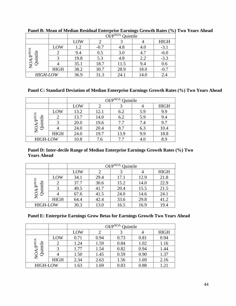
Panels C and D report that earnings growth forecasted by NOAP

NOA is risky. For a given

enterprise E/P, the standard deviation of realized enterprise earnings growth rates is increasing in

enterprise B/P in panel C, as is the inter-decile range (the 90th percentile minus the 10th percentile

of outcomes) in panel D. The inter-decile range is of particular significance because it focuses on

the extreme outcomes about which investors are presumably most concerned.

Panel E reports betas (slope coefficients) from time-series regressions, for each portfolio, of

two year ahead earnings growth rates on the market-wide earnings growth rate for the same year.

These “earnings growth betas” are increasing in enterprise B/P for a given enterprise E/P

portfolio. Not only is the earnings growth of high B/P portfolios more volatile (Panels C and D),

they are also more sensitive to systematic shocks to growth. The reported earnings growth betas

in panel E are based on earnings growth rates for the median firm in each cell. In unreported

tests we have repeated the estimation of earnings growth betas using aggregate earnings growth

across all firms in each cell. This approach will give considerably more weight to larger firms

who are less subject to aggregate market shocks. As expected we see similar, albeit reduced,

differences in earnings growth betas across the 25 cells using this alternative estimation

approach.

23

Panel F reports the fraction of firms that ceased to exist in the second year ahead due to

performance-related reasons, as indicated by CRSP delisting codes.20 The non-survivor rates are

higher for the low E/P portfolio dominated by loss firms, but are also higher for the high B/P

portfolios. Across all panels in the table we see that high enterprise B/P firms are subject to more

extreme earnings growth outcomes as evidenced by (i) the dispersion in portfolio level measures

of earnings growth, and (ii) the sensitivity of growth to shocks to market-wide earnings growth,

and (iii) the higher percentage of non-survivors due to either low payoffs attributable to firm

failure and/or high payoffs due to firms being acquired by other firms.

In summary, given OI/PNOA, NOAP

NOA indicates not only expected earnings growth (panels A

and B) but also the risk surrounding the expected growth (panels C - F). Not only is P1 supported

empirically, but the risk surrounding the expected growth is also related toNOAP

NOA. The analysis is

on an unlevered basis as a prelude to the analysis that adds leverage later, but results are similar

with portfolios formed on levered E/P and B/P with levered earnings growth outcomes.

5. Estimating Characteristic Regressions

5.1 Regressions with Levered Explanatory Variables

The test of P1 confirms the condition in our framework for B/P to indicate expected returns.

With this condition satisfied, we now proceed to P2: for a given E/P, is B/P correspondingly

related to expected returns? While the variation of earnings growth rates in table 4 indicates that

B/P is associated with risky growth outcomes, the risk need not be priced risk. As is standard in

empirical asset pricing, we use average realized returns to infer expected returns that reflect

priced risk. That is, the test of P2 is under the maintained assumption of market efficiency (as is

standard). With our interest in the FF model (with levered B/P), the focus at this point is on

levered E/P and B/P.

Table 5 reports results from estimating regression equations (8) and variants. Cross-

sectional regressions are estimated each year, and the reported coefficients and R2 are averages

20 In unreported tests, we have also examined the fraction of firms that do not have the requisite data to compute

earnings growth in the subsequent year. The pattern is very similar to that reported in panel F.

24

of estimates across years, with t-statistics calculated as the average coefficient estimate relative

to its standard error estimated from the time-series of the coefficients. In unreported analysis we

have estimated all regression specifications using monthly returns rather than annual returns,

with similar results.

Regression I shows that B/P is significantly positively associated with future returns, as is

well known. Regression II estimates equation (8): both E/P and B/P jointly indicate future

returns, with significantly positive coefficients on both variables. The adjusted R2 is an

improvement over that in Regression I with B/P alone. Regression III adds the current dividend-

to-price (D/P). All else equal, dividends reduce future earnings, so the inclusion of D/P helps

correct the forecast of forward earnings for the current payout. Adding D/P also controls for any

tax effects of dividends on returns and the possibility that D/P itself is an indicator of expected

returns via expected dividend growth. The coefficient on D/P is negative, consistent with

earnings displacement, but it is not significant, taking nothing away from E/P and B/P as

expected return characteristics.

Regression IV adds beta and size, the other FF characteristics, to Regression III. Size has

a significant negative coefficient, with E/P and B/P retaining their significance, while beta is

insignificant. Note also that our measure of forward earnings is only an estimate, so any variable

that improves that estimate has a role in the regression regardless of whether it indicates

subsequent earnings growth.

The results for these regressions are consistent over sub-periods—1962-1975, 1976-1985,

1986-1995, and 1996-2013—though the weight on E/P is higher in the earlier periods and the

weight on B/P higher in the later periods. In summary, regression specifications I to IV support

B/P as a valid characteristic, as in the FF model, but also indicates that E/P is missing from that

model.

The analysis in Table 4 indicates a non-linearity across unlevered E/P portfolios in the

relationship between unlevered B/P and subsequent earnings growth. To assess the robustness of

the results in Table 5 to the linearity assumption underlying the regression analysis (and also to

check on the influence of outliers), we also calculated mean t+1 returns from investing in the

portfolios in Table 4, and also for portfolios similarly constructed from a joint sort on levered

25

E/P and B/P rather than their levered components. We merely summarize the results here; the

detail is available on request.

In both cases, average returns are increasing in the E/P ratios, with a significant

difference between the high and low E/P portfolios. Further, mean returns are also increasing in

B/P for each of the E/P portfolios (both for the levered and unlevered ratios), with significant

differences in mean returns between high and low B/P for a given E/P. In short, the returns align

with the growth rates for the portfolios in Panels A and B of Table 4 and also with the measures

of the risk around the growth in Panels C - D of Table 4.

For these same portfolios, we also calculated “alphas” (estimated intercepts) from

estimates of Fama and French time-series factor regressions with three factors and with four

factors (including momentum). The significant intercepts observed confirm that the relation

between B/P and E/P and future returns in our portfolios cannot be explained by the standard set

of factors; the joint sort based on the characteristics identified by our framwork exposes

meaningful variation in realized returns that cannot be explained by FF factor models. Again,

results are available on request.

5.1.1 Relative importance of E/P and B/P in explaining expected returns

While these regressions indicate that both E/P and B/P typically predict returns in the cross-

section, our framework demonstrates that, in the case of no expected earnings growth, only E/P

is relevant. B/P takes on significance only with expected earnings growth, and only when that

growth is at risk of not meeting expectations. Accordingly, we now partition the cross-section

into firms where a priori one expects different levels of expected earnings growth.

Our instrument for expected earnings growth is firm size. This is admittedly a crude

proxy, based on the intuition that smaller firms are typically those with higher growth (and

riskier) prospects while large firms are those where growth expectations have largely been

achieved.21 But there is another reason to partition in size: the FF model includes size as a

21 In unreported results we have used alternative, non-market based measures of firm size. Specifically, we partition

firms into deciles based on book equity and book net operating assets. A challenge with using accounting based

measures of size is that the very same accounting principles that give rise to risky earnings future earnings growth

also affect current accounting estimates in the balance sheet. Conservative accounting creates low estimates of

balance sheet values for business models with risky investment activity, thus sorting on book estimates of size can

26

characteristic as well as B/P (and size loads negative in Regression IV in table 5). However,

rather than viewing size as another characteristic that indicates returns incrementally to B/P, we

view size as a condition under which the weight on E/P in predicting returns shifts to B/P.

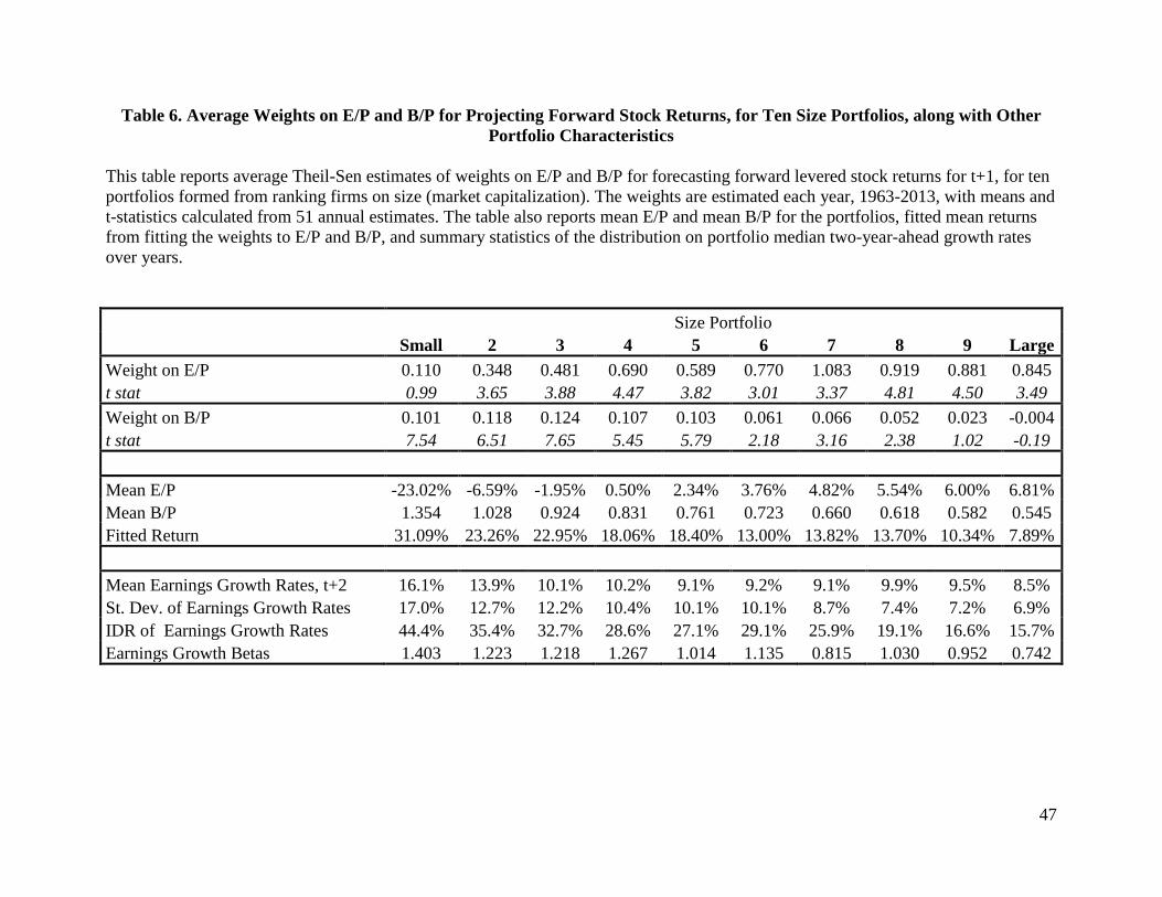
We estimate weights on E/P and B/P for size partitions using the Theil-Sen robust

estimator advocated by Ohlson and Kim (2014). These weights are the median values of w1 and

w2 from fitting PBwPEwRt // 211 for all possible combinations of observations. Table 6

reports the average weights for ten portfolios formed each year from a ranking on firm size.22

The weight on E/P increases with firm size, and approaches to 1.0 for the largest portfolios, the

weight appropriate for no growth under our framework. Correspondingly, the weight on B/P

decreases with firm size, effectively zero for the larger firms. For smaller firms (where higher

growth is expected), the weight shifts from E/P to B/P, again consistent with our framework. The

table also reports mean E/P and B/P for the portfolios, with E/P increasing over portfolios and

B/P decreasing. The fitted returns in the table are calculated by applying the weights to E/P and

B/P for the portfolio (with an intercept). These returns are decreasing in firm size, consistent

with the standard observation that average returns are negatively related to size.23 The last four

rows of the table report the same statistics for two-year-ahead realized growth rates as in Table 4.

It is clear that the weight on B/P and the associated fitted returns are increasing in the portfolio

mean growth rates, their variation around the mean, and their sensitivity to market-wide shocks.

The results here are consistent with observations (in Kothari, Shanken and Sloan, 1995

and Asness, Frazzini, Israel, and Moskowitz, 2015, for example) that the B/P effect in stock

returns is considerably weaker for large firms. But now a rationale is supplied, one that points to

E/P for these firms rather than B/P. Andrade and Chhaochharia (2014) observe that E/P rather

than B/P explains returns for large firms; again, a rationale is supplied here.

confound the issue. That said, we see similar, albeit slightly weaker, relations using book equity and book net

operating assets to partition on size.

22 In a comparison with OLS coefficients, there is considerably less variation in the estimates over years, attributed

to extreme values having less influence.

23 These mean returns should not be interpreted as ex ante expected returns. Realized returns over this sample period

(to which the weights were fitted) were those in an (on average) bull market. Indeed, the fitted returns are (on

average) higher than what one typically views as a reasonable required return. This is particularly so for the small

firms for, in this period, investing in risky growth paid off.

27

It has been observed that the FF portfolio sorts on B/P also imbed a size sort that

obscures the weak B/P effect in large firms (in Lambert and Hübner, 2013 and Asness, Frazzini,

Israel, and Moskowitz, 2015, for example). Consequently, there appears to be a B/P effect in

large firms in FF only because the sort on B/P is actually a sort on size. The analysis here goes

further, to question whether size and B/P are two separate characteristics. Size and B/P are

clearly negatively correlated over portfolios in table 6, and both are associated with risky growth

outcomes. Thus both may be seen as a characteristic that correlates with returns. However, our

framework and table 6 promotes only B/P as a characteristic, but one that receives a higher

weight with smaller firms because smaller firms have higher, riskier growth expectations.

To be sure, firm size is but one of many potential characteristics that could be used to

identify firms with greater expectations of risky future earnings growth. One simple alternative

is to directly measure investment activity that is immediately expensed, but which produces

expected earnings growth from that investment over the initial reduced earnings. The two most

common, and measurable, such investment activities are research and development (R&D)

expenditures and advertising expenditures. In unreported analysis, we have repeated the analysis

in table 6 but instead sort firms on the intensity of R&D and advertising expenditures. We

assume a useful life of three years for R&D and one year for advertising, and deflate this simple

measure of ‘intangible’ assets by either sales or net operating assets. The results are very similar

to that reported in table 6: for firms with greater intangible asset intensity, B/P is more important

in explaining expected returns. This is expected in our framework as the conservative nature of

the accounting system defers the recognition of earnings associated with this risky investment

activity. In such situations, E/P is no longer a sufficient statistic for expected returns.

Overall, the findings in table 6 confirm the insight from our identification framework that

both E/P and B/P identify expected returns. There is, however, an inconsistency with the results

in Fama and French (1992) who suggest that E/P is not significant in monthly cross sectional

after controlling for size, beta, and B/P. Our analysis here suggests an explanation. As observed,

the FF sorts confound size and B/P such that the return spread within large firms is attributed to

B/P rather than size. While confirming the insignificance of B/P for large firms, table 6 also

28

shows that E/P and size are positively correlated over size portfolios. Thus, for large firms where

E/P is particularly important, size proxies for E/P.24

5.2 Regressions with Unlevered Explanatory Variables and Added Leverage

In this section, we attempt to validate our identification approach by revisiting the puzzling

negative relation between financial leverage and future equity returns observed in previous

papers. The negative relation has been attributed to a failure to control for operating risk

characteristics appropriately. So, we test whether a positive relation is now observed after

controlling for the operating risk characteristics identified.

We start by confirming that the negative relation observed earlier holds for our sample.

Regression I in table 7 reports the estimates of benchmark FF regression (11). As in Penman,

Richardson, and Tuna (2007), there is a negative relation between financial leverage and future

returns. In unreported analysis, we split each cross-section based on whether NOAP

NOA is greater

than or less than one, that is, around the “kink” in equation (5). As in Penman, Richardson, and

Tuna (2007), the negative leverage relation is strongest for NOAP

NOA less than one where the

majority of firms lie and where leverage decreases B/P; the average coefficient on leverage (not

reported in the table) is -0.030 with an associated test statistic of -3.22. Adding beta and size to

the regressions does not alter the picture, and thus the conclusion remains that the FF model does

not accommodate leverage risk.

24 Holding aside the modelling supporting our analysis, it is important to reconcile our empirical tests with those of

Fama and French (1992). If we (i) restrict our time period to their sample period,1963-1990, (ii) compute ‘E’ and

‘B’ consistent with Fama and French (1992), (iii) use the same lagging conventions (i.e., use financial statement data

from the most recent fiscal year-end no later than December of year t when looking at returns that start in July of

year t+1), (iv) include an indicator variable for negative firms and only compute E/P for firms where E > 0, and (v)

use monthly return intervals as opposed to the annual return intervals, we continue to find that both B/P and E/P are

associated with the cross section of future stock returns. It is only when we (i) require all components of ‘E’ and ‘B’

as measured by Fama and French (1992) to be non-missing (i.e., non-missing income statement deferred taxes,

preferred dividends, and balance sheet deferred taxes), and (ii) include all firms (i.e., do not remove securities with

closing share price of less than $0.20) that we can find a sub-sample where, empirically at least, E/P is not

significant in explaining future stock returns. This is not surprising as the smallest firms are those firms with the

largest expectations for earnings growth, and one would expect B/P to be more important as it captures those

expectations of subsequent earnings growth.

29

Regression II adds the enterprise (unlevered) earnings yield, the missing operating

characteristic identified, to the benchmark regression, as in equation (10). The mean coefficient

on leverage is now close to zero. The addition of unlevered size and beta in Regression III does

not change this coefficient significantly. These findings are similar when excluding firms with

operating losses and those with negative net debt (that is, cash-rich firms). They also hold for

various sub-periods from 1962-2013.25

However, the analysis in section 2.3 indicates there is an interaction effect between

leverage and operating risk to be accommodated. The remaining regressions in table 7 recognize

these points by exploiting E/P leveraging equation (4). Regressions IV and V introduce the kink

in equation (4) around the enterprise earnings yield equal to the borrowing rate with the

condition for the leverage effect on the levered E/P to be favorable, NOAP

OI> Rf. We use the 10-

year U.S. Treasury rate, Rf, as the threshold borrowing rate given the scarcity of quality

corporate borrowing cost data back in time. ForNOAP

OI> Rf in regression IV, the average

coefficient on leverage is positive. Further, the average coefficient on the interaction variable in

Regression V is reliably positive. Applying the estimated coefficients to the average values of

both the leverage and the interaction variable in the cross-section, we find that the total effect of

leverage is positive with an associated test statistic (not tabulated) of 2.74. Overall and in

contrast to the typical finding in the literature, the analysis indicates a positive conditional

relation between leverage and future equity returns.

The coefficients on the leverage variables in these regressions could be attributable to

leverage being related to additional omitted aspects of operating risk. But our data suggest

otherwise. First, there is a very low correlation between leverage and future unlevered returns in

table 2. Second, in unreported tests we estimate regression II in table 7 using unlevered returns

as the dependent variable. We find a weak negative relation (test statistic of -1.34), suggesting

(weakly) that firms with higher (lower) leverage have lower (higher) operating risk. The

25 We also split on NOAP

NOA is greater than or less than one, that is, around the “kink” in equation (5). For

NOAP

NOA > 1,

the mean coefficient on leverage was marginally significant for the appropriate one-tail test, but not for NOAP

NOA< 1.

30

weakness of the relation and its negative sign suggest that the positive conditional relation that

we document between leverage and future levered returns cannot easily be explained by leverage

capturing operating risk.

5.2.1 Leverage in Ex Post Return Regressions

The regressions in Table 7 are not very powerful for identifying differences in expected returns.

Indeed, while the reported R2 are higher than typically observed for return regressions, they are

still quite low. As often observed, the reason is that realized returns are a poor metric to detect

small differences in expected returns because the variation in realized returns due to the

unexpected return component is far greater than that of the expected return component (see e.g.,

Elton, 1999), and the relative contribution of leverage to the expected return is typically small.

To increase the power of the tests, we repeat the analysis, but now with a control for the

contemporaneous earnings news that explains part of the unexpected component of realized

returns. The analysis also permits a sharper definition of favorable and unfavorable leverage

where the directional effect of leverage on returns differs. We estimate the following regression

equation:

1432

1

11

t

t

t

NOA

t

t

NOA

t

t

NOA

t

tt

P

ND

P

NOA

P

OI

P

OIR

(12)

The inclusion of realized enterprise earnings,NOA

t

t

P

OI 1 , controls for unexpected returns due to the

contemporaneous realization of earnings news. We also include lagged enterprise earnings,

NOA

t

t

P

OI, because extensive prior research shows that both earnings levels and changes explain

realized stock returns (in Easton and Harris 1991, for example).

Table 8 reports the results. Regression I reports the results from estimating equation

(12). There is a positive coefficient on the realized earnings yield and a significant increase in

average R2 over the regressions reported in table 7. This reinforces the point that expected

earnings are at risk so that their realizations determine realized returns. The average coefficient

on lagged earnings is negative, indicating that lower prior earnings for a given earnings

31

realization—realized earnings growth—is associated with higher returns. This is implied by our

framework where expected earnings growth is at risk, so realizations of growth move returns.

After controlling for earnings realizations, there is a positive but still insignificant association

between leverage and future returns.

However, the effect of leverage on returns depends on whether leverage is favorable;

leverage levers up realized returns if outcomes are favorable, but reduces returns if not. So, the

remaining regressions in table 8 partition on the earnings realization. Regression II excludes

firms with operating losses and the remaining regressions examine cases with earnings

realizations greater than and less than the borrowing rate (proxied by the 10-year Treasury rate),

the inflection point for favorable and unfavorable leverage in equation (4). Regressions are run

with and without leverage interaction terms. For regressions III – V that we identify with

favorable leverage, the coefficient on leverage is strongly positive and the overall effect of the

leverage term and the interaction term is positive. In unreported analysis, we estimate regression

II excluding the main effect for leverage and find the coefficient on the interaction variable is

0.909 with a test statistic of 4.81.

Regression VI attempts to capture the case of “unfavorable” leverage. However, an

interaction term cannot be calculated when operating income is negative (the most demonstrable

case of an unfavorable outcome), so we include a loss dummy variable. The average coefficient

on leverage is negative but not statistically different from zero. Thus we don’t observe a negative

leverage effect directly. But the coefficient is considerably less than that for regression III

covering favorable earnings outcomes.

In unreported analysis, we also estimated the regressions by defining favorable outcomes

as OIt+1 > OIt and unfavorable ones as OIt+1 < OIt. For regression I for favorable news, the

coefficient on leverage was 0.035 with a t-statistic of 2.72, while that for unfavorable news was

-0.016 with a t-statistic of -2.14. The interaction coefficient in regression II for favorable news

was 1.244 (t = 3.16) and that for unfavorable news was -0.004 (t = -0.02). In regression V (that

excludes the leverage main effect term), the coefficient on the interaction term was 0.77 (t =

4.16) for favorable news and -0.026 (t = -0.15) for unfavorable news. In summary, after

controlling for operating risk characteristics and the contemporaneous earnings news, we can

32

identify a robust positive relation between leverage and future returns, albeit asymmetric, with

the relation stronger in the cases we have identified leverage as favorable.

These regressions emphasize the ex post nature of leverage. Given the negative relation

between leverage and returns typically observed in prior research, the results are important. But

they also shows that our framework identifies a characteristic regression model where leverage is

priced positively.

6. Conclusion

This paper develops a framework for identifying characteristics that indicate expected returns.

Expected returns can be described in terms of expected forward earnings and subsequent

earnings growth under conditions prescribed by accounting principles. Characteristics that

indicate expected earnings and subsequent earnings growth that are at risk also indicate the

expected return for bearing that risk, assuming the market prices risk efficiently.

The paper takes the framework to a critique of asset pricing models where book-to-price

appears as a characteristic. We establish accounting conditions under which B/P indicates

expected returns and those where it does not. The conditions under which B/P is a valid risk

characteristic involve a particular form of accounting that resembles GAAP. We test empirically

whether these conditions are satisfied. Our framework and the accompanying empirical tests

show that B/P indicates expected returns because it forecasts expected earnings growth and the

risk that the expectation may not be met. In one sense, the paper justifies B/P in the Fama and

French asset pricing model. However, it also identifies E/P as missing from the Fama and French

model. Indeed, when there is no expected earnings growth, it is E/P that indicates expected

returns and B/P is irrelevant. With expected earnings growth, the weight shifts to B/P, and does

progressively more so with smaller firms where growth expectations are presumably higher.

While the focus is on pricing models with B/P, the framework in the paper is quite general for

identifying characteristics that pertain to risk and return. For example, Penman and Zhu (2014)

take the framework developed in this paper to investigate a number of “anomalies” that have

appeared in empirical analysis.

The framework identifies characteristics that indicate the expected return due to operating

risk versus those that indicate the financing risk premium in expected returns. The paper shows

33

that operating and financing risk characteristics combine to explain the (levered) equity return in

the same way that unlevered stock returns and leverage combine to yield the levered equity

return under Modigliani and Miller (1958). With the separation of operating and financing risk,

we document a positive relation between returns and leverage. This contrasts with prior research

that has consistently found a negative relation between leverage and equity returns, a finding

inconsistent with basic principles of finance. We attribute the earlier negative relation as a failure

to identify operating risk characteristics appropriately. Our finding of a positive relation further

validates our framework.

The paper is written under the assumption that markets rationally price risk, as is standard

in asset pricing in identifying characteristics that indicate risk and return; in order to address this

research, we must be on the same platform. However, we indicate the expected returns for risk

only under this assumption. As always in empirical asset pricing, our empirical findings (and

those in asset pricing research more generally) could be attributed to inefficient pricing if the

characteristics predict returns because the market fails to incorporate information about future

earnings and subsequent earnings growth. Our documentation that the predicted returns are

associated with fundamental (earnings) risk relieves the concern, but the paper in no way

resolves the long-standing debate about market efficiency. That, of course, requires a valid factor

model, but the paper holds out the prospect of developing such a model, one that comes from an

accounting-based framework.

34

References

Andrade, S., and V. Chhaochharia. 2014. Is there a value premium among large stocks?

Unpublished paper, University of Miami.

Asness, C., A. Frazzini, R. Israel, and T. Moskowitz. 2015. Fact, fiction, and momentum

investing. Journal of Portfolio Management 42, 34-52.

Berk, J., R. Green, and V. Naik. 1999. Optimal investment, growth options, and security returns.

Journal of Finance 54, 1153-1608.

Bhandari, L. 1988. Debt/equity ratio and expected common stock returns: Empirical evidence.

Journal of Finance 43, 507-528.

Bradshaw, M., S. Richardson, and R. Sloan. 2001. Do analysts and auditors use information in

accruals? Journal of Accounting Research 39, 45-74.

Carlson, M., A. Fisher, and R. Giammarino. 2004. Corporate investment and asset pricing

dynamics: Implications for the cross-section of returns. Journal of Finance 56, 2577-2603.

Caskey, J., J. Hughes, and J. Liu. 2012. Leverage, excess leverage, and future returns. Review of

Accounting Studies 17, 443-471.

Chan, L., J. Karceski, and J. Lakonishok. 2003. The level and persistence of growth rates. The

Journal of Finance 58, 643-684.

Chen, H. 2017. Do cash flows of growth stocks really grow faster? Journal of Finance 72, 2279-

2330.

Chen, L., R. Petkova, and L. Zhang. 2008. The expected value premium. Journal of Financial

Economics 87, 269-280.

Cochrane, J. 1991. Production-based asset pricing and the link between stock returns and

economic fluctuations. Journal of Finance 46, 209-237.

Cochrane, J. 1996. A cross-sectional test of an investment-based asset pricing model. Journal of

Political Economy 104, 572-621.

Cooper, M., H. Gulen, and M. Schill. 2008. Asset growth and the cross-section of stock returns.

The Journal of Finance 63, 1609-1651.

Easton, P., and T. Harris. 1991. Earnings as an explanatory variable for returns. Journal of

Accounting Research 29, 19-36.

Easton, P., T. Harris, and J. Ohlson. 1992. Aggregate accounting earnings can explain most of

security returns: The case of long event windows. Journal of Accounting and Economics 15

(June-September), 119-142.

35

Elton, E. 1999. Expected return, realized return, and asset pricing tests. Journal of Finance 54,

1999-1220.

Fama, E., and K. French. 1992. The cross-section of expected stock returns. Journal of Finance

47, 427-465.

Fama, E., and K. French. 1993. Common risk factors in the returns of stocks and bonds. Journal

of Financial Economics 33, 3-56.

Fama, E., and K. French. 1995. Size and book-to-market factors in earnings and returns. Journal

of Finance 50, 131-155.

Fama, E., and K. French. 2015. A five-factor asset pricing model. Journal of Financial

Economics 116, 1-22.

Francis, J., R. LaFond, P. Olsson, and K. Schipper. 2005. The market pricing of accruals quality.

Journal of Accounting and Economics 39, 295-327.

George, T., and C. Hwang. 2010. A resolution of the distress and leverage puzzles in the cross

section of stock returns. Journal of Financial Economics 96, 56-79.

Gomes, J., L. Kogan, and L. Zhang. 2003. Equilibrium cross-section of returns. Journal of

Political Economy 111, 693-732.

Gomes, J., and L. Schmid. 2010. Levered returns. Journal of Finance 65, 467-494.

Green, J., J. Hand, and F. Zhang. 2013. The supraview of return predictive signals. Review of

Accounting Studies 18, 692-730.

Green, J., J. Hand, and F. Zhang. 2014. The remarkable multidimensionality in the cross-section

of expected U.S. stock returns. Unpublished paper, University of North Carolina at Chapel Hill.

Harvey, C., Y. Liu, and H. Zhu. 2016. … and the cross-section of expected returns. Review of

Financial Studies 29, 5-68.

Hou, K., C. Xue, and L. Zhang. 2015. Digesting anomalies: An investment approach. Review of

Financial Studies, 28, 650-705.

Hughes, J., J. Liu, and W. Su. 2008. On the relation between predictable market returns and

predictable analysts’ forecast errors. Review of Accounting Studies 13, 266-291.

Ippolito, F., R. Steri, and C. Tebaldi. 2011. The relative leverage premium. Working paper,

Bocconi University, at http://ssrn.com/abstract=1762116.

Jegadeesh, N., and S. Titman. 1993. Returns to Buying Winners and Selling Losers: Implications

for Stock Market Efficiency. The Journal of Finance 48, 65-91.

36

Johnson, T. 2004. Forecast dispersion and the cross section of expected stock returns. Journal of

Finance 59, 1957-1978.

Lakonishok, J., A. Shleifer, and R. Vishny. 1994. Contrarian investment, extrapolation, and risk.

The Journal of Finance 49, 1541-1578.

Lambert, M., and G. Hübner. 2013. Comoment risk and stock returns. Journal of Empirical

Finance and Stock Returns 23, 191-205.

Leland, H. 1994. Corporate debt value, bond covenants, and optimal capital structure. The

Journal of Finance 49, 1213-1252.

Lin, X., and L. Zhang. 2013. The investment manifesto. Journal of Monetary Economics 60,

351-366.

Liu, L., T. Whited, and L. Zhang. 2009. Investment-based expected stock returns. Journal of

Political Economy 117, 1105-1139.

Lyle, M., J. Callen, and R. Elliott. 2013. Dynamic risk, accounting-based valuation and firm

fundamentals. Review of Accounting Studies 18, 899-929.

Lyle, M. and C. Wang. 2015. The cross section of expected holding period returns and their

dynamics: A present value approach. Journal of Financial Economics 116, 505-525.

Miller, M., and F. Modigilani. 1961. Dividend policy, growth and the valuation of shares.

Journal of Business, 34 (October), 411-433.

Modigliani F., and M. Miller. 1958. The cost of capital, corporation finance and the theory of

investment. American Economic Review 48, 261-297.

Nielsen, A. 2006. Corporate governance, capital structure choice and equity prices. Working

paper, Princeton University, at http://ssrn.com/abstract=882055.

Novy-Marx, R. 2012. The other side of value: The gross profitability premium. Journal of

Financial Economics 108, 1-28.

Novy-Marx, R. 2014. Prediciting anomaly performance with politics, the weather, global

warming, sunspots, and the stars. Journal of Financial Economics 112, 137-146.

Obreja, I. 2013. Book-to-market equity, financial leverage and the cross-section of stock returns.

Review of Financial Studies 26, 1146-1189.

Ohlson, J. 1995. Earnings, book values, and dividends in equity valuation. Contemporary

Accounting Research 12, 661-687.

Ohlson, J. 2008. Risk, growth, and permanent earnings. Unpublished paper, New York

University Stern School of Business.

Ohlson, J., and B. Juettner-Nauroth. 2005. Expected EPS and EPS growth as determinants of

value. Review of Accounting Studies 10, 349-365.

37

Ohlson, J., and S. Kim. 2014. Linear valuation without OLS: the Theil-Sen estimation approach.

Review of Accounting Studies, forthcoming. Published online at Springer Link, June 2014.

Penman, S. 1992. An evaluation of accounting rate-of-return. Journal of Accounting, Auditing,

and Finance 6, 233-255,

Penman, S. 1996. The articulation of price-earnings ratios and market-to-book ratios and the

evaluation of growth. Journal of Accounting Research 34, 235-259.

Penman, S., and F. Reggiani. 2013. Returns to buying earnings and book value: Accounting for

growth and risk. Review of Accounting Studies 18, 1021-1049.

Penman, S., S. Richardson, and İ. Tuna. 2007. The book-to-price effect in stock returns:

Accounting for leverage. Journal of Accounting Research 45 (May), 427-467.

Penman, S., and J. Zhu. 2014. Accounting Anomalies, Risk and Return. The Accounting Review

89, 1835-1866.

Shroff, P. 1995. Determinants of the returns-earnings correlation. Contemporary Accounting

Research 12 (Fall), 41-55.

Shumway, T., 1997. The delisting bias in CRSP data. The Journal of Finance, 52, 327 – 340.

Skogsvik, K., S. Skogsvik, and H. Thorsell. 2011. Disentangling the enterprise book-to-price and

leverage effects in stock returns. Unpublished paper, Stockholm School of Economics.

Wahlen, J., and M. Wieland. 2011. Can financial statement analysis beat analysts’

recommendations? Review of Accounting Studies 16, 89-115.

Zhang, L. 2005. The value premium. Journal of Finance 60, 67-103.

38

Figure 1. Average enterprise earnings growth rates two years ahead (t+2) for portfolios

formed from joint sorts of the enterprise earnings yield (OI/PNOA) and enterprise book-to-

price (NOA/PNOA) at time t.

See notes to Tables 1 and 4 for the calculation of variables.

39

Table 1. Distribution of Variables

This table reports selected percentiles of variables from data pooled over firms and years, 1962-

2013, along with averages and standard deviations. For the calculation of averages and standard

deviations, the top and bottom 2 percent of variables each year were excluded, except for returns.

Percentiles Returns Unlevered

Returns

E/P B/P OI/PNOA NOA/PNOA ND/P

1 -0.888 -1.281 -2.103 -0.811 -1.134 -0.090 -1.074

2 -0.817 -0.968 -1.177 -0.168 -0.634 -0.013 -0.722

5 -0.679 -0.697 -0.487 0.056 -0.289 0.037 -0.409

10 -0.529 -0.480 -0.211 0.139 -0.132 0.114 -0.239

25 -0.250 -0.176 -0.015 0.304 0.003 0.332 -0.060

50 0.042 0.055 0.047 0.571 0.048 0.657 0.153

75 0.366 0.296 0.086 0.984 0.078 0.980 0.669

90 0.826 0.744 0.140 1.586 0.118 1.314 1.695

95 1.281 1.285 0.186 2.135 0.154 1.610 2.895

98 2.091 2.480 0.254 3.032 0.222 2.171 5.674

99 2.944 4.071 0.316 3.904 0.301 2.865 9.234

Average 0.156 0.111 -0.005 0.751 0.017 0.710 0.516

Std. Dev. 0.810 0.537 0.244 0.617 0.142 0.449 1.056

Accounting data are from Compustat and returns and price data are from CRSP. Financial firms are excluded. There

is a maximum of 170,096 firm-years in the calculations, though less for some variables.

Returns, Rt+1, are buy-and-hold returns for twelve months beginning three months after the end of fiscal-year t,

calculated from CRSP monthly returns. For firms that are delisted during the return period, the remaining return for

the period was calculated by first applying CRSP’s delisting return and then reinvesting any remaining proceeds in a

size-matched portfolio (where size is measured as market capitalization at the start of the return accumulation

period). This mitigates concerns about potential survivorship bias. Firms that are delisted for poor performance

(CRSP delisting codes 500 and 520–584) frequently have missing delisting returns, in which case a delisting return

of −100% was applied. Final accounting data for a fiscal year are presumed to have been published during the three

months after fiscal-year end (and before the beginning of the return period).

Unlevered returns, NOA

tR 1, are enterprise returns for the same annual period as the levered stock returns, calculated as

NOA

t

NOA

tt

NOA

t PPFCFP /)( 11 , with

tt

NOA

t NDPP where ND is the book value of net debt as an approximation to

its market value. Free cash flow, FCFt+1 = OIt+1 – (NOAt+1 – NOAt), according to the clean surplus equation for

operating activities. For the calculation of operating income, OI, and net operating assets NOA, see below.

Unlevered returns are calculated on a total dollar basis (rather than with per-share amounts).

E/P is an estimate of the forward earnings yield, tt PEarningsE /)( 1, with forward earnings forecast as earnings

before extraordinary items (Compustat item IB) and special items (SPI) for the prior year, year t, minus preferred

dividends (DVP), with a tax allocation to special items at the prevailing statutory corporate income tax rate for the

40

year. Earnings and prices are on a per-share basis, with prices observed three months after fiscal-year end, adjusted

for stock splits and stock dividends during the three months following fiscal-year end.

B/P, the (levered) book-to-price ratio, is book value of common equity at the end of the current fiscal-year t, divided

by price at t. Book value is Compustat’s common equity (CEQ) plus any preferred treasury stock (TSTKP) less any

preferred dividends in arrears (DVPA). Book values and prices are on a per-share basis, with prices observed three

months after fiscal-year end, adjusted for stock splits and stock dividends during the three months following fiscal-

year end.

OI/PNOA is an estimate of the forward unlevered (enterprise) earnings yield, NOA

tt POIE /)( 1, with forward enterprise

earnings (operating income) forecast as operating income for the prior year calculated as earnings (as above) plus

net interest expense and preferred dividends with a tax allocation to net interest at the prevailing statutory tax rate

for the year.

NOA/PNOA is unlevered (enterprise) book-to-price. Net operating assets is book value of equity plus book value of

net debt. See below for the calculation of net debt.

ND/P is market leverage at the end of fiscal-year t, with the market value of debt approximated by its book value,

ND. Net debt is the sum of long-term debt (Compustat item DLTT), debt in current liabilities (DLC), carrying value

of preferred stock (PSTK), preferred dividends in arrears (DVPA), less preferred treasury stock (TSTKP), all

reduced by financial assets (“excess cash”) measured as cash and short-term investments (CHE)

41

Table 2. Average Pearson and Spearman Correlations Between Variables

This table reports average cross-sectional correlations for the period 1962-2013. Reported correlations are averages of annual

correlation coefficients across the 52 years in the sample period. Pearson correlations are presented in the upper diagonal and Spearman

correlations in the lower diagonal. For the Pearson correlations, the top and bottom 2 percent of observations for each variable are

discarded each year with the exception of returns, beta, and size.

See notes to Table 1 for calculation of variables. Betas, estimated from a maximum of 60 monthly returns and a minimum of 24

monthly returns prior to the period beginning three months after firms’ fiscal-year end, are from market model regressions using CRSP

value-weighted market return inclusive of all distributions. Size is the natural log on equity market capitalization.

Returns Unlevered

Returns

E/P B/P OI/PNOA NOA/PNOA ND/P Beta Size

Returns 0.568 0.058 0.080 0.076 0.072 0.009 -0.021 -0.031

Unlev Ret 0.643 0.100 0.075 0.138 0.083 -0.025 -0.014 0.028

E/P 0.176 0.182 0.082 0.784 0.112 -0.103 -0.130 0.231

B/P 0.118 0.104 0.292 0.115 0.878 0.315 -0.115 -0.291

OI/PNOA 0.173 0.211 0.896 0.234 0.147 -0.098 -0.116 0.208

NOA/PNOA 0.105 0.119 0.279 0.908 0.204 0.384 -0.152 -0.243

ND/P 0.010 0.018 0.063 0.257 -0.095 0.462 -0.073 -0.111

Beta -0.052 -0.031 -0.174 -0.144 -0.126 -0.164 -0.109 -0.017

Size 0.055 0.070 0.196 -0.267 0.189 -0.244 -0.029 0.005

42

Table 3. Average Median Earnings Growth Rates Two Years Ahead for Portfolios Formed

by Ranking Firms on Book-to-Price and Enterprise Book-to-Price

Panel A reports means of median realized earnings growth rates and residual earnings growth

rates two years ahead for ten portfolios formed each year, 1963-2013, by ranking firms on book-

to-price, B/P. Panel B reports mean of median enterprise earnings growth rates and residual

enterprise earnings growth rates for portfolios formed by ranking firms each year on enterprise

book-to-price, NOA/PNOA.

Portfolios are formed from ranking all firm observations each calendar year, 1963-2013, on

book-to-price, B/P (Panel A) and enterprise book-to-price, NOA/PNOA (Panel B). Cut-offs for

the portfolios were determined from the ranking in the prior year. Variables are defined in Table

1. Firms with negative book values are excluded.

Reported growth rates are averages of median portfolio t+2 growth rates over years, 1962-2013.

To accommodate negative denominators, earnings growth rates are calculated as

2/)( 12

2

tt

t

EarningsEarnings

Earnings , and similarly so for operating (enterprise) income, OI. This measure

ranges between 2 and -2. Residual earnings are calculated as Earningst+2 – (Rf × Bt+1) and

residual OI in calculated as OIt+2 – (Rf × NOAt+1), with the growth rate over t+1 calculated in the

same way as the earnings growth rate. Rf is the yield on the U.S. 10-year Treasury note for the

respective year.

Panel A: Mean of Median Earnings Growth Rates and Residual Earnings Growth Rates

Two Years Ahead, in Percent

B/P Decile

LOW 2 3 4 5 6 7 8 9 HIGH HIGH-

LOW

Earnings 8.8 9.1 9.0 8.0 9.2 8.6 9.5 10.7 14.1 19.0 10.2

Residual

Earnings 2.2 3.5 4.4 4.6 6.6 7.0 10.0 12.9 17.4 24.3 22.1

Panel B: Mean of Median Enterprise Earnings (OI) Growth Rates and Residual Enterprise

Earnings Growth Rates Two Years Ahead, in Percent

NOA/PNOA Decile

LOW 2 3 4 5 6 7 8 9 HIGH HIGH-

LOW

OI 6.6 10.8 9.9 9.2 9.1 9.6 9.1 10.0 12.1 15.0 8.4

Residual

OI -0.4 3.7 3.3 3.5 2.8 5.5 8.2 14.6 21.6 22.5 22.9

43

Table 4. Average Median Enterprise Earnings Growth Rates Two Years Ahead and

Variation in Growth Rates, for Portfolios Formed from Joint Sorts of the Enterprise

Earnings Yield and Enterprise Book-to-Price

Panel A reports the mean of median realized enterprise earnings growth rates two years ahead for

portfolios formed each year, 1963-2013, on enterprise earnings yield, OI/PNOA and enterprise

book-to-price, NOA/PNOA. Panel B reports corresponding residual earnings growth rates. Panel

C reports the standard deviation of portfolio growth rates over the years, and Panel D reports the

inter-decile range of growth rates. Panel E reports betas (slope coefficients) from a time-series

regression of median portfolio growth rates two years ahead on the market-wide median growth

rate for that year. Panel F gives non-survivor rates for the portfolios.

Portfolios are formed from ranking all firm observations each calendar year, 1963-2013, first on

enterprise earnings-to-price, OI/PNOA, and then, within each OI/PNOA portfolio, on enterprise

book-to-price, NOA/PNOA. Cut-offs for the portfolios are determined from the ranking in the

prior year. Variables are defined in Table 1. Firms with negative values of PNOA are excluded.

Reported growth rates in Panels A and B are means of median portfolio growth rates across

years. Standards deviations and inter-decile ranges in Panels C and D refer to portfolio growth

rates across years. To accommodate negative denominators, growth rates are calculated as

2/)( 12

2

tt

t

OIOI

OI where OI is operating (enterprise) income, calculated as in the notes to Table 1.

This growth rate ranges between 2 and -2. Residual enterprise earnings in Panel B is calculated

as OIt+2 – (Rf × NOAt+1), with the growth rate over t+1 calculated in the same way as the OI

growth rate. Rf is the yield on the U.S. 10-year Treasury note for the year.

The betas (slope coefficients) in Panel E are from a time-series regression of portfolio growth

rates two years ahead on the market-wide growth rate for that year. The market-wide growth rate

is calculated using all firms in the sample for a given year. To align in calendar time, these betas

were estimated using only firms with December 31 fiscal-year ends.

Non-survivors in Panel F are those with delisting codes 500, 520, 550, 551, 552, 560, 561, 570,

572, 574, 575, 580, 581, 582, 583, 584, 585, 587, 589, and 591 on CRSP.

Panel A: Mean of Median Enterprise Earnings Growth Rates (%) Two Years Ahead

OI/PNOA Quintile

LOW 2 3 4 HIGH

NO

A/P

NO

A

Quin

tile

LOW 6.6 7.6 10.9 8.6 4.0

2 14.1 12.4 11.2 8.7 3.5

3 23.3 14.5 12.0 7.7 3.7

4 33.4 19.3 11.7 8.6 5.0

HIGH 37.0 23.0 14.9 9.4 3.4

HIGH-LOW 30.4 15.5 4.0 0.9 -0.6

44

Panel B: Mean of Median Residual Enterprise Earnings Growth Rates (%) Two Years Ahead

OI/PNOA Quintile

LOW 2 3 4 HIGH

NO

A/P

NO

A

Quin

tile

LOW 1.2 -0.7 4.8 4.0 -3.1

2 9.4 0.5 3.0 4.7 -6.0

3 19.8 5.3 4.8 2.2 -3.3

4 35.1 18.7 11.5 9.4 0.6

HIGH 38.2 30.7 28.9 18.0 -0.7

HIGH-LOW 36.9 31.3 24.1 14.0 2.4

Panel C: Standard Deviation of Median Enterprise Earnings Growth Rates (%) Two Years Ahead

OI/PNOA Quintile

LOW 2 3 4 HIGH

NO

A/P

NO

A

Quin

tile

LOW 13.2 12.1 6.2 5.9 9.9

2 13.7 14.0 6.2 5.9 9.4

3 20.0 19.6 7.7 7.4 9.7

4 24.0 20.4 8.7 6.3 10.4

HIGH 24.0 19.7 13.9 9.9 18.8

HIGH-LOW 10.8 7.6 7.7 4.0 8.9

Panel D: Inter-decile Range of Median Enterprise Earnings Growth Rates (%) Two

Years Ahead

OI/PNOA Quintile

LOW 2 3 4 HIGH

NO

A/P

NO

A

Quin

tile

LOW 34.1 29.4 17.1 12.9 21.8

2 37.7 30.6 15.2 14.0 22.9

3 49.5 41.7 20.4 15.5 21.5

4 67.6 41.5 24.0 14.6 24.1

HIGH 64.4 42.4 33.6 29.8 41.2

HIGH-LOW 30.3 13.0 16.5 16.9 19.4

Panel E: Enterprise Earnings Grow Betas for Earnings Growth Two Years Ahead

OI/PNOA Quintile

LOW 2 3 4 HIGH

NO

A/P

NO

A

Quin

tile

LOW 0.71 0.94 0.73 0.81 0.94

2 1.24 1.59 0.84 1.02 1.16

3 1.77 1.54 0.82 0.94 1.44

4 1.50 1.45 0.59 0.90 1.37

HIGH 2.34 2.63 1.56 1.69 2.16

HIGH-LOW 1.63 1.69 0.83 0.88 1.21

45

Panel F: Fraction (%) of Firms Delisted Between Year t+1 and t+2 for Performance

Related Reasons

OI/PNOA Quintile

LOW 2 3 4 HIGH

NO

A/P

NO

A

Quin

tile

LOW 6.21 1.63 0.43 0.30 0.56

2 7.20 2.07 0.39 0.31 0.63

3 7.34 2.34 0.72 0.41 0.54

4 8.02 3.01 0.95 0.77 1.00

HIGH 6.29 3.47 2.17 1.39 1.51

HIGH – LOW 0.08 1.84 1.74 1.09 0.95

46

Table 5. Average Coefficient Estimates and Test Statistics for Levered Characteristic

Regressions

This table reports average coefficients estimates from 52 annual cross-sectional regressions of

forward stock returns (for t+1) on time-t levered characteristics, along with t-statistics and

average adjusted R-square, 1962-2013.

Reported coefficients are averages from yearly cross-sectional regressions for the years, 1962-

2013. The t-statistics, reported in parentheses below the average coefficient estimates, are the

average coefficient divided by a standard error estimated from the time series of coefficient

estimates. To minimize the influence of outliers, the top and bottom two percent of the

explanatory variables were deleted each year. Variables are defined in notes to Table 1 and Table

2. The divide yield is dividends per share for year t divided by price at the end of year t, dpst/Pt.

I

II

III

IV

Intercept 0.081

(2.72)

0.069

(2.26)

0.081

(2.52)

0.152

(3.70)

E/P

0.348

(2.52)

0.478

(2.75)

0.401

(2.68)

B/P 0.103

(5.97)

0.092

(5.51)

0.096

(5.29)

0.069

(4.58)

Size -0.013

(-2.72)

Beta 0.009

(0.68)

Div. Yield -0.866

(-1.48)

-0.536

(-1.44)

Adj-R2 0.015 0.026 0.039 0.055

# Firm-Years 170,096 166,022 164,381 140,838

47

Table 6. Average Weights on E/P and B/P for Projecting Forward Stock Returns, for Ten Size Portfolios, along with Other

Portfolio Characteristics

This table reports average Theil-Sen estimates of weights on E/P and B/P for forecasting forward levered stock returns for t+1, for ten

portfolios formed from ranking firms on size (market capitalization). The weights are estimated each year, 1963-2013, with means and

t-statistics calculated from 51 annual estimates. The table also reports mean E/P and mean B/P for the portfolios, fitted mean returns

from fitting the weights to E/P and B/P, and summary statistics of the distribution on portfolio median two-year-ahead growth rates

over years.

Size Portfolio

Small 2 3 4 5 6 7 8 9 Large

Weight on E/P 0.110 0.348 0.481 0.690 0.589 0.770 1.083 0.919 0.881 0.845

t stat 0.99 3.65 3.88 4.47 3.82 3.01 3.37 4.81 4.50 3.49

Weight on B/P 0.101 0.118 0.124 0.107 0.103 0.061 0.066 0.052 0.023 -0.004

t stat 7.54 6.51 7.65 5.45 5.79 2.18 3.16 2.38 1.02 -0.19

Mean E/P -23.02% -6.59% -1.95% 0.50% 2.34% 3.76% 4.82% 5.54% 6.00% 6.81%

Mean B/P 1.354 1.028 0.924 0.831 0.761 0.723 0.660 0.618 0.582 0.545

Fitted Return 31.09% 23.26% 22.95% 18.06% 18.40% 13.00% 13.82% 13.70% 10.34% 7.89%

Mean Earnings Growth Rates, t+2 16.1% 13.9% 10.1% 10.2% 9.1% 9.2% 9.1% 9.9% 9.5% 8.5%

St. Dev. of Earnings Growth Rates 17.0% 12.7% 12.2% 10.4% 10.1% 10.1% 8.7% 7.4% 7.2% 6.9%

IDR of Earnings Growth Rates 44.4% 35.4% 32.7% 28.6% 27.1% 29.1% 25.9% 19.1% 16.6% 15.7%

Earnings Growth Betas 1.403 1.223 1.218 1.267 1.014 1.135 0.815 1.030 0.952 0.742

48

Table 7. Average Coefficient Estimates and Test Statistics for Unlevered Characteristic

Regressions

This table reports average coefficients estimates from 52 annual cross-sectional regressions of

forward stock returns (for t+1) on time t operating characteristics and leverage, along with t-

statistics and average adjusted R-square, 1962-2013.

See notes to Table 5. Unlevered size is the natural log of enterprise market capitalization,

measured as equity market capitalization plus the book value of net debt (in millions of dollars).

Rf is the yield on the U.S. 10-year Treasury note for the relevant year. All other variables are

defined in notes to Table 1 and Table 2. Firms with negative values of PNOA are excluded.

I

II

III

IV

OI/PNOA>Rf

V

OI/PNOA>Rf

Intercept 0.069

(2.13)

0.050

(1.55)

0.139

(3.34)

0.028

(0.83)

0.045

(1.40)

OI/PNOA

0.655

(3.39)

0.546

(3.53)

1.364

(5.13)

1.176

(5.04)

NOA/PNOA 0.126

(6.12)

0.093

(4.60)

0.070

(3.58)

0.029

(1.55)

0.029

(1.52)

UnLevSize -0.015

(-2.71)

Beta 0.011

(0.77)

ND/P

-0.017

(-2.15)

-0.002

(-0.21)

0.000

(0.04)

0.036

(2.17)

-0.046

(-1.60)

OI/PNOA*ND/P 1.018

(2.71)

Adj-R2

# Firm-Years

0.018

164,657

0.032

160,929

0.057

138,147

0.021

56,808

0.022

56,808

49

Table 8. Average Coefficient Estimates and Test Statistics for Characteristic Regressions with Realized Returns and Realized

Earnings

This table reports average coefficients estimates from 51 annual cross-sectional regressions of stock returns for year t+1on the

contemporaneous realized enterprise earnings yield for the same year, leverage and other characteristics, along with t-statistics and

average adjusted R-square, 1962-2012.

Reported coefficients are averages from yearly cross-sectional regressions for the years, 1962-2012. The t-statistics, reported in

parentheses below the average coefficient estimates, are the average coefficient divided by a standard error estimated from the time

series of coefficient estimates. To minimize the influence of outliers, the top and bottom two percent of the explanatory variables were

deleted each year. Variables are defined in notes to Table 1 and Table 2. Firms with negative values of PNOA are excluded. ILOSS is an

indicator variable equal to one when OIt+1 < 0, and zero otherwise. NOA

tt POI /1 is the realized operating income in year t+1 relative

enterprise price at t and Rf is the yield on the U.S. 10-year Treasury note for the relevant year.

I

II NOA

tt POI /1> 0

III NOA

tt POI /1>Rf

IV NOA

tt POI /1>Rf

V NOA

tt POI /1>Rf

VI NOA

tt POI /1<Rf

Intercept 0.028

(0.86)

-0.009

(-0.33)

0.034

(0.91)

0.064

(1.83)

0.047

(1.31)

0.016

(0.46) NOA

tt POI /1 2.652

(8.26)

4.461

(15.28)

4.596

(11.10)

4.252

(12.47)

4.407

(11.90)

2.147

(2.97) NOA

tt POI / -1.747

(-6.73)

-2.361

(-8.98)

-2.535

(-8.66)

-2.468

(-9.05)

-2.428

(-9.29)

-1.353

(-4.71)

NOA

tt PNOA /

0.085

(4.23)

-0.008

(-0.41)

-0.044

(-2.06)

-0.043

(-1.97)

-0.052

(-2.14)

0.039

(1.33)

NDt/Pt 0.007

(0.70)

-0.052

(-2.78)

0.084

(5.68)

-0.072

(-2.32)

-0.010

(-0.68) NOA

tt POI /1*ND/P 1.468

(4.22)

1.616

(3.39)

1.009

(4.83)

ILOSS -0.068

(-1.46)

Adj-R2 0.134 0.183 0.153 0.167 0.161 0.099

No. of Firm-Years 149,972 115,852 61,311 61,311 61,311 88,661