Universit ` a degli Studi di Pisa Facolt` a di Scienze Matematiche, Fisiche e Naturali Corso di Laurea Magistrale in Informatica A Framework to compare text annotators and its applications October 2012 Master Degree Thesis Candidate Marco Cornolti [email protected]Supervisor Prof. Paolo Ferragina [email protected]Universit` a di Pisa Co-Reviewer Prof.ssa Anna Bernasconi [email protected]Universit` a di Pisa Academic Year 2011/2012
Transcript
Universita degli Studi di Pisa
Facolta di Scienze Matematiche, Fisiche e Naturali
Texts in human languages have a low logical structure and are inherently am-
biguous because of this structure and the presence of polysemous terms. Never-
theless, the typical approach of Information Retrieval to manage text documents
has been, up to now, based on the Bag-of-words model (BoW) [38]. In this
model, texts are represented as the multi-set of terms they contain, thus dis-
carding any possible structure or positional relations existing among the terms.
Moreover, terms are interpreted as sequence of characters and mapped to inde-
pendent dimensions into a huge Euclidean space, so that synonymy and poly-
semy issues are not taken into account at all. Because of its simplicity, BoW
is at the core of most (if not all) current text retrieval systems; but anyone is
aware of its obvious limitations.
Recently, some research groups tried to overcome these limitations by propos-
ing a novel approach which consists of adding some “contextual information”
to text representation, identifying meaningful mentions in the input text and
linking them to their corresponding topics provided by a proper ontology. See
Figure 1.1 for an example. This process is nowadays called “text annotation”
and the software systems which implement it are called “topic annotators” or
“topic-retrieval systems”. These systems differ to each other by the ontology
used to extract the annotated concepts (E.g. Wordnet [10], CiC [24], Wikipedia,
Yago 2 [16]) and by the algorithms employed to derive these annotations.
The power of these systems resides in the underlying structure which in-
terconnects the topics attached to the texts within the ontology. The most
successful systems are currently the ones based on Wikipedia, and these sys-
tems have been applied to improve the performance of IR tools on many classic
problems such as: the categorization or the clustering of documents; the topic-
3
based search over a web collection, and so on.
The success in the use of Wikipedia lies in the fact that this online ency-
clopedia offers free (as in freedom) and open access to a huge knowledge base
that, despite not being guaranteed to be correct, provides a very high quality
thanks to the process used to author Wikipedia pages [22]. Wikipedia is open
to the contribute of everyone, including anonymous users, and pages authoring
is collaborative. The lack of a central authority potentially leads to a low reli-
ability, but since the review process is distributed as well, involuntary mistakes
or malicious errors are quickly found and corrected [25].
Wikipedia is a huge mine of semi-structured information. First of all, Wiki-
pedia pages can be seen as a representation of specific and unambiguous topics.
Their abstract and their content give a detailed description of the topic, meta-
data like the hits count and the revisions give information about the popularity
of the concept and how frequently its description changes, pages are catego-
rized by a rich set of categories, and anchors of links to a Wikipedia page offer
a set of commonly used synonyms for the concept the page is about. But
the most interesting information lies into the structure of its graph, where the
nodes are the Wikipedia pages and the edges are the links between pages: the
shape of the graph can tell much about how semantically close two pages are
[31, 40, 12, 15, 34].
Many topic-retrieval systems use this direct graph, and the whole informa-
tion that Wikipedia offers, to solve synonymy and polysemy issues in the input
text [14, 28, 5, 8, 9]. The approaches followed by the systems differ in the way
this information is exploited.
Our Contribution
These systems give surprisingly good results, but the research have followed
specific and target-oriented trends, leading to disuniform terminology and ap-
proaches, despite targeting the same set of problems. To address the research,
it is fundamental to have a consistent framework that offers a formal base upon
which it’s possible to build new theories, algorithms and systems.
Moreover, there is no improvement without measuring, and literature gives
a plenty of ways to determine the performance of a system. Unfortunately, the
used methods are inconsistent with each other.
The aim of this thesis is to formalize such a framework, presenting both
some of the problems related to topic-retrieval and a set of measures to assess
the performance of the systems in solving those problems. The result of this
work is a benchmarking framework software that performs the measures on the
systems.
4
Figure 1.1: An example of a topic retrieval task: from the un-structured texton the left, the unambiguous topics are extracted.
In Chapter 2, we discuss the formal framework, presenting the problems
related to topic-retrieval. To solve the lack of uniformity in the measures, our
contribution is the presentation in Chapter 3 of a set of metrics that can be used
to fairly compare the topic annotators to each other. Despite sounding straight-
forward, the definition of this metrics hides non-trivial issues. The implemented
benchmarking software based on these metrics is presented in Chapter 4.
In Chapter 5 a snapshot of the state-of-the-art topic annotators is given,
as well as the available datasets to perform the benchmarking. Results of the
benchmark of these annotators on the dataset are given in Chapter 6 and show
that some systems, like TagMe, Illinois Wikifier and Wikipedia Miner, give good
results with a rather low runtime, suggesting their application to large-scale
datasets.
In Chapter 7 some lines of possible future development are presented.
To facilitate the reading of this thesis, all defined formulas are reported in a
table in Appendix A, with a brief description.
5
Chapter 2
Some topic retrieval
problemsWhat’s in a name? that which we call a rose
By any other name would smell as sweet.
– William Shakespeare, Romeo and Juliet, Act II
2.1 Terminology
As stated in the Introduction, literature about topic retrieval presents a wide
variability of terminologies. The following terminology, that will be used in the
next chapters of this thesis, is a compromise between the popularity of a term
in literature, its clarity, and the avoidance of conflicts with other works that
may lead to ambiguity.
• A concept is a Wikipedia page. It can be uniquely identified by its Page-ID
(an integer value).
• A mention is the occurrence of a sequence of terms located in a text. It
can be codified as a pair 〈p, l〉 where p is the position of the occurrence
and l is the length of the sub-string including the sequence of terms.
• A score is a real value s ∈ R, s ∈ [0, 1] that can be assigned to an
annotation or a tag. Higher values of the score indicate that the annotation
(or tag) is more likely to be correct.
• A tag is the linking of a natural language text to a concept and is codified
as the concept c the text refers to. A tag may have a score: a scored tag
is encoded as a pair 〈c, s〉, where s is the score.
6
This thesis Milne-Witten[33]
Han-Sun-Zhao[13]
Ferragina etal. [11]
Ratinov et al.[36]
Meij et al. [27]
concept sense entity sense Wikipedia ti-tle
concept
mention anchor name mention spot mention
tag annotation
annotation link entity linking annotation mapping
score score ρ-score score
Table 2.1: Terminology used by some of the works in literature.
• An annotation is the linking of a mention in a natural language text to a
concept. It can be codified as a pair 〈m, c〉 where m is the mention and c
is the concept. An annotation may have a score: a scored annotation can
be codified as 〈m, c, s〉, where s is the score.
Table 2.1 reports a “vocabulary” of the different terminology used in other
publications.
2.2 Definition of problems
We define a set of problems related to the retrieval of concepts in natural lan-
guage texts. The difference between these problems can be seen as subtle but
leads to different approaches to measure the performance of a topic-retrieval
system. The definition of the problems related to topic retrieval is given in Ta-
ble 2.2, where each problem comes with the type of the input (that is, the type
of a problem instance) and output (the type of the solution). Figure 2.1 shows
some examples of input and correct output for the given problems.
2.2.1 The topic-retrieval problems and their applications
Problems presented Table 2.2 face different applications. Let’s give some shallow
examples. For a document clustering based on the document topics, we are
interested in finding only the tags, and not the annotations of a document, hence
this application would depend on the the solution of C2W and its scored variant
Sc2W. Successful applications of this problem are presented in [18, 20, 39].
Rc2W, that returns concepts ordered by the likelihood that they are correct,
can as well be used. Applications such as user profiling and document retrieval
are as well based on these problems.
Annotations are useful for assisting human reading. Reading a text, like
an article on an on-line newspaper, the meaning of some mentions could be
unclear. Annotating the text adding a link from these mentions to the right
7
Problem Input Output Description
Disambiguate to Wikipedia(D2W)
Text,Set ofmen-tions
Set of annotationsthat, to each men-tion given as input,assign a (possiblynull-) concept.
Given a list of men-tions, find the concept ex-pressed by each mention(null if the concept couldnot be found). This prob-lem has been defined in[36].
Concepts to Wikipedia (C2W) Text Set of tags Identify the set of con-cepts that are explicitlymentioned in a text.
Scored concepts to Wikipedia(Sc2W)
Text Set of scored tagswith distinct con-cepts
Identify the set of con-cepts that are explicitlymentioned in a text. Tagsare assigned a score rep-resenting the likelihoodthat the tag is correct.
Annotate to Wikipedia (A2W) Text Set of annotations Identify the relevant men-tions of the text andthe concepts expressed bythose mentions.
Scored-annotate to Wikipedia(Sa2W)
Text Set of scored anno-tations
Identify the relevant men-tions of the text andthe concepts expressed bythose mentions. Annota-tions are assigned a scorerepresenting the likeli-hood that the annotationis correct.
Ranked-concepts to Wikipedia(Rc2W)
Text List of tags Identify the set of con-cepts that are cited in atext. The concepts areranked by the probabilitythat the concept is cor-rect.
Table 2.2: Description of topic-retrieval problems
8
Figure 2.1: Examples of instances of the topic-retrieval problems and theircorrect solution. Mentions are highlighted in red, (scored) tags in blue, (scored)annotations in green. Concepts are in italics.
9
Reduction Instance adaptation Solution adaptation
A2W ∝ Sa2W No adaptation. discard the scores, take only the concepts with ascore higher than a given threshold.
D2W ∝ A2W Take only the text,discard the mentions.
let M be the set of mentions to disambiguate, partof the instance. Take only the annotations 〈m, c〉 ofthe solution such that m ∈ M . Set the concept ofall other mentions in M to null.
Sc2W ∝ Sa2W No adaptation. Discard the mentions, take only the concepts andtheir score. Let A = a1, · · · , an be the solution ofproblem Sa2W. If two annotations ai and aj havethe same concept, discard the one with lower score.
Rc2W ∝ Sc2W No adaptation. Take only the concepts with a score higher than agiven threshold. Rank the concepts by their score,discard the scores.
C2W ∝ Rc2W No adaptation. Turn the list into a set.
C2W ∝ A2W No adaptation. Discard the mentions, take only the set of concepts.
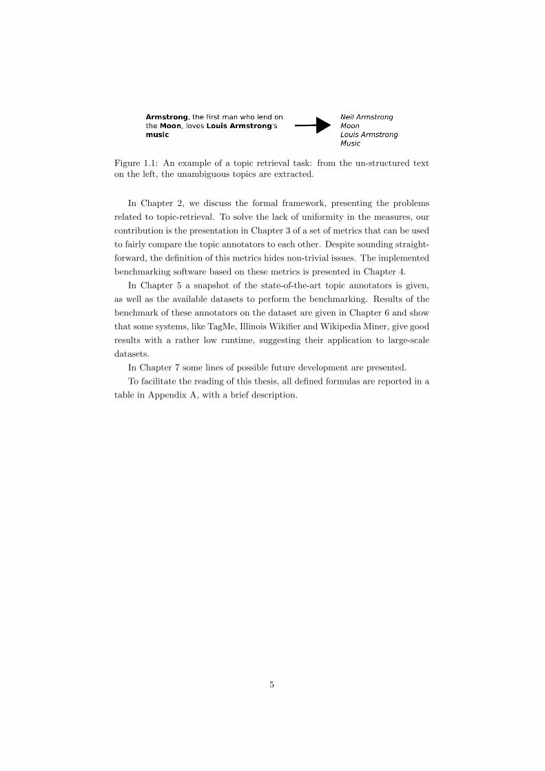
Table 2.3: Reduction between problems. A ∝ B means A can be reduced to B(hence B is harder than A).
Wikipedia concept would help a human understand the text. This is called text
augmenting and lies upon the solution of A2W and its scored variant Sa2W.
D2W could also be used for this application, interactively asking the human
user which mentions should be annotated.
2.3 Our contribution: A hierarchy of problems
It is of key importance to note that the defined problems are strictly related
to each other, and some of them can be reduced to others. Note that A ∝ B
indicates that A reduces to B, so that an instance IA of A can be adapted in
polynomial time to an instance IB of B and a solution SB of B can be adapted
in polynomial time to a solution SA of A. In this case, we say that B is harder
than A, since an algorithm that solves B also solves A. For a presentation of
the reduction theory, see [7].
Let’s give an example. If a solution SA2W for the A2W problem is found, it
can be adapted in polynomial time (O(n) where n is the size of the output) to
a solution SC2W of the C2W problem, by simply discarding the mentions and
leaving the retrieved concepts. The instance IC2W of the problem C2W does
not even need any adaptation to fit to problem A2W, since both problems have
texts as instances (thus IA2W = IC2W and the adaptation is O(1)).
We can safely assume the reductions presented in Table 2.3.
Keeping in mind that the reduction between problems is transitive and re-
flexive, this leads to a hierarchy of problems illustrated by the graph in Figure
10
Figure 2.2: Preordering of the reductions between problems.
2.2. The most general problems is Sa2W, and all other problems reduce to it.
Problems D2W and C2W are the most specific. The complete chains in the
preordering of the problems are:
C2W ∝ Rc2W ∝ Sc2W ∝ Sa2W
C2W ∝ A2W ∝ Sa2W
D2W ∝ A2W ∝ Sa2W
Throwing a rope to the next chapters, it is fundamental to point out that,
for the purpose of benchmarking the annotation systems, the performance of
two systems S′ (solving problem P ′) and S′′ (solving problem P ′′) can be fairly
compared only if they respectively solve P ′ and P ′′, and there is a problem P
such that P ∝ P ′ ∧ P ∝ P ′′. In this hypothesis, the evaluation can be done
with respect to the ability of systems S′ and S′′ to solve problem P . Since
the preordering of the reductions is reflexive, obviously two systems can be
compared if they both solve problem P or if they solve respectively P ′ and P ′′,
and P ′ ∝ P ′′.Keeping an eye on the graph in Figure 2.2, note that the performances of
systems S′ and S′′ in solving problem P can be compared if and only if a
reverse-path exists from problem P to P ′ and from problem P to P ′′.
Also note that, if P ′ ∝ P ′′, a dataset giving a gold standard (i.e. an expected
output) for P ′′ can be adapted to be used as a gold standard for P ′, using the
same techniques presented in Table 2.3.
11
2.4 Conclusions
This chapter has presented the basic terminology that will be used in the follow-
ing chapters. We also presented the first part of the formal framework, defining
a set of problems related to topic retrieval. These problems show different fea-
tures, but can be framed into a preordering representing the reduction between
them. This lets two systems natively solving two different problems P ′ and P ′′
be fairly compared to each other with respect to their ability to solve a third
problem P such that P ∝ P ′ ∧ P ∝ P ′′.
12
Chapter 3
New evaluation metricsWe judge ourselves by what we feel capable of doing,
while others judge us by what we have already done.
– Henry Wadsworth Longfellow, Kavanagh: A Tale.
The issue of establishing a baseline, shared by the community, to evaluate
the performance of systems that solve the problems presented in Chapter 2 is of
crucial importance to help the development of new algorithms and to address
the research in this field. In this chapter, some metrics for the evaluation of
correctness are proposed. The aim is to establish a set of experiments that fairly
evaluate the performance of a system (Section 3.1) and evaluate how similar two
systems are (Section 3.4). The performance of a system mainly depends on four
factors:
1. The ability of the system in recognizing the mentions (for problems Sa2W
and A2W).
2. The ability of the system in assigning a set of candidate concepts to each
mention (for problems Sa2W, A2W and D2W) or to the whole text (Sc2W,
Rc2W, C2W);
3. The ability of the system in selecting the right concept (disambiguation);
4. The ability of the system in assigning the score (for problems Sc2W,
Sa2W) or the ranking (for Rc2W) to the annotations or tags.
While Section 3.1 presents a set of metrics to evaluate the performance of
the full chain of these abilities (1-4) for all problems, some of them can be tested
in-depth and separately: Section 3.2 focuses the metrics on the evaluation of
finding mentions (ability 1), while metrics presented in Section 3.3 evaluates the
ability of finding the right concepts (abilities 2 and 3).
13
3.1 Metrics for correctness evaluation
Experiments are performed checking the output of the tagging systems against
the gold standard given by a dataset. Of course, for each problem a different
set of metrics has to be defined. This section covers all the problems presented
in Chapter 2. Classical measures like the true positives, false positives, false
negatives, precision and recall are generalized and built on top of a set of binary
relations. These binary relations represent a match between two tags or two
annotations. The necessity of the generalization comes from the need that two
annotations or tags, to be considered as matching, do not need to be equal
but, more generally, have to satisfy a match relation. Things will be clearer
continuing the reading of the next subsections. In the meanwhile, the following
definitions are given:
Definition 1 Let X be the set of elements such that a solution of problem P
is a subset of X. Let r ⊆ X be the output of the system for an instance I of
problem P , g ⊆ X be the gold standard given by the dataset for instance I and
M a symmetric match relation on X. The following higher-order functions are
defined:
true positives tp(r, g,M) = {x ∈ r | ∃x′ ∈ g : M(x′, x)}false positives fp(r, g,M) = {x ∈ r | 6 ∃x′ ∈ g : M(x′, x)}false negatives fn(r, g,M) = {x ∈ g | 6 ∃x′ ∈ r : M(x′, x)}true negatives tn(r, g,M) = {x 6∈ r | 6 ∃x′ ∈ g : M(x′, x)}
Generally, a dataset offers more than one instance. Thus, an output of a
system checked against all the instances provided by a dataset consists of a list
of results, one for each instance. The following commonly used metrics [26] are
re-defined, generalized with the matching relation M .
Definition 2 Let G = [g1, g2, · · · , gn] be the gold standard given by a dataset
that contains n instances I1, · · · , In, given as input to a system, gi being the
gold standard for instance Ii. Let R = [r1, · · · , rn] be the output of the system,
where ri is the result found by the system for instance Ii. The following metrics
are defined:
14
precision P (r, g,M) = |tp(r,g,M)||tp(r,g,M)|+|fp(r,g,M)|
Note that, if the binary relation M is the equality (M(a, b) ⇔ a = b), the
measures presented above become the classical Information Retrieval measures.
Now that this layer of metrics have been defined, we can play on the match
relation M .
3.1.1 Metrics for the C2W problem
For the C2W problem, the match relation to use is quite straightforward. The
output of a C2W system is a set of tags. Keeping in mind that a tag is codified
as the concept it refers to, the following definitions are given:
Definition 3 Let T be the set of all tags. A Strong tag match is a binary
relation Mt on T between two tags t1 and t2. It is defined as
Mt(t1, t2)⇐⇒ d(t1) = d(t2)
Where d is the dereference function (see Definition 4)
Definition 4 Let L be the set of redirect pages, C be the set of non-redirect
pages (thus C ∩ L = ∅) in Wikipedia. Dereference is a function
d : L ∪ C ∪ {null} 7→ C ∪ {null}
such that:
d(p) =
p if p ∈ C
p′ if p ∈ L
null if p = null
where p′ ∈ C is the page p redirects to.
15
Definition 3 and the dereference function worth an explanation. In Wikipe-
dia, a page can be a redirect to another, e.g. “Obama” and “Barrack Hussein
Obama” are redirects to “Barack Obama”. Redirects are meant to ease the
finding of pages by the Wikipedia users. Redirects can be seen as many-to-one
bindings from all synonyms (pages in L) to the most common form of the same
concept (pages in C). Two concepts identified by c1 and c2, where c1 6= c2 but
d(c1) = d(c2) (meaning that c1 redirects to c2 or that c1 and c2 redirect to the
same page c3) represent the same concept and thus must be considered as equal.
It is obvious that the Strong tag match relation Mt is reflexive (∀x ∈T. Mt(x, x)), symmetric (Mt(y, x) ⇔ Mt(x, y)), and transitive (Mt(x, y) ∧Mt(y, z)⇒Mt(x, z)).
To achieve the actual metrics for the C2W problem, the number of true/false
positives/negatives, precision, recall and F1 must be computed according to
Definitions 1 and 2, using M = Mt.
3.1.2 Metrics for the D2W problem
D2W output consists of a list of annotations, some of them possibly with null -
concept. To compare two annotations, the following match function, as well
reflexive, symmetric and transitive, is given.
Definition 5 Let A be the set of all annotations. A Strong annotation match
is a binary relation Ms on A between two annotations a1 = 〈〈p1, l1〉, c1〉 and
a2 = 〈〈p2, l2〉, c2〉 . It is defined as
Ms(a1, a2)⇐⇒
p1 = p2
l1 = l2
d(c1) = d(c2)
Where d is the dereference function (see Definition 4).
Note that in D2W it does not make sense to count the negatives, since
the mentions of the annotations contained in the output are the same as the
mentions given as input, and only the concepts can be either correct (true
positive) or wrong (false positive). To compute the number of true and false
positives, as long as the precision, functions defined in Definition 1 and 2 can
be used, with M = Ms.
3.1.3 Metrics for the A2W problem
As in D2W, the output of a A2W problem is a set of annotations. The main
difference is that in A2W the mentions are not given as input and must be found
by the system.
16
A possible set of metrics for A2W would be analogue to those given in Defi-
nitions 1 and 2 with M = Ms (Definition 5). But the Strong annotation match
will result to be true only if the mention matches perfectly, and this approach
leaves aside some cases of matches that should still be considered as right. Sup-
pose a A2W annotator is given as input the sentence “The New Testament is the
basis of Christianity”. A correct annotation returned by the annotation system
could be 〈〈4, 13〉,New Testament〉 (correctly mapping the mention “New Testa-
ment” to the concept New Testament). But suppose the gold standard given by
the dataset was another similar and correct annotation 〈〈0, 17〉,New Testament〉(mapping the mention “The New Testament” to the same concept). Since the
mentions differ, a metric based on the Strong annotation match would count
one false positive and one false negative, whereas only one true positive should
be counted. Definition 5 can be relaxed as described in Definition 6 to match
annotations with overlapping mentions and same concept.
Definition 6 Let A be the infinite set of all annotations. A Weak annotation
match is a binary relation Mw on A between two annotations a1 = 〈〈p1, l1〉, c1〉and a2 = 〈〈p2, l2〉, c2〉. Let e1 = p1 + l1 − 1 and e2 = p2 + l2 − 1 be the indexes
of the last character of the two mentions. The relation is defined as
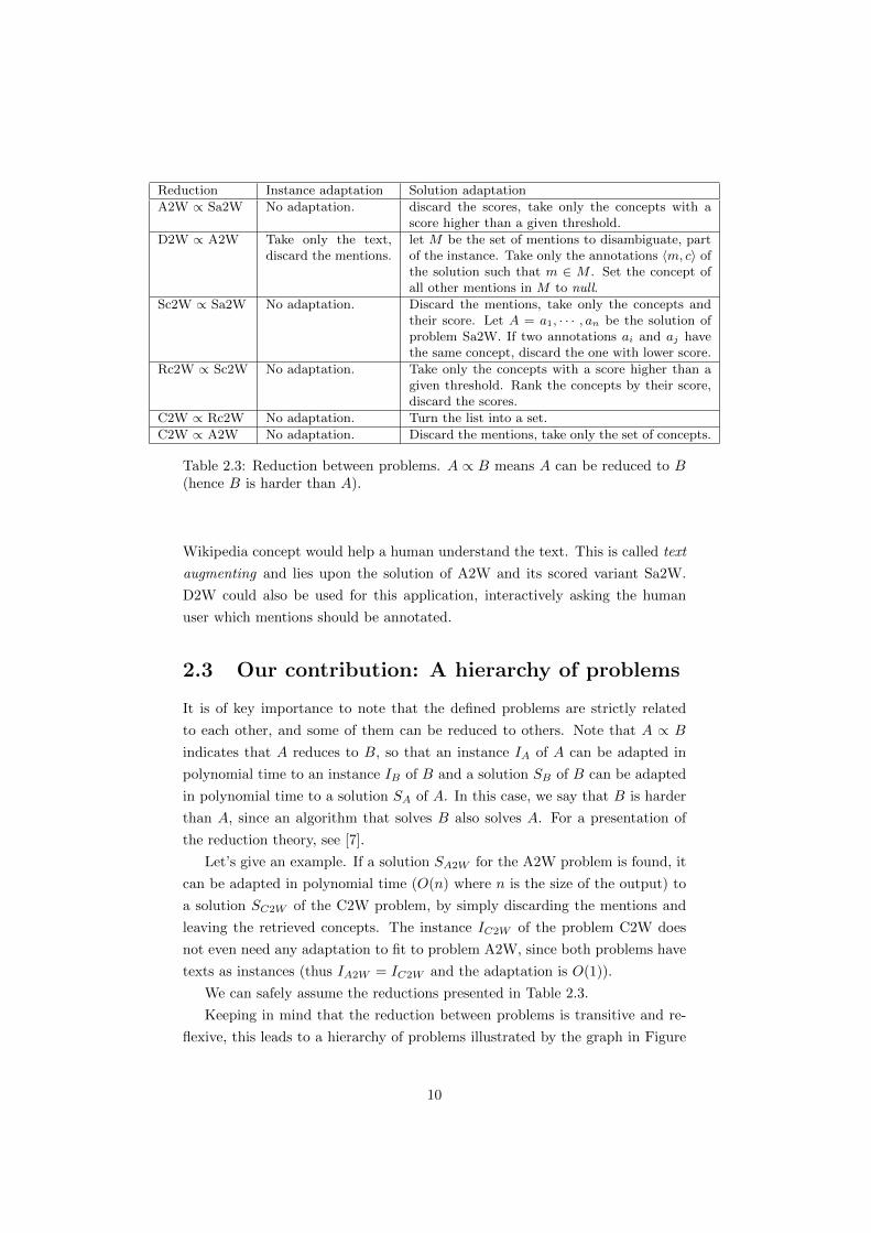
Smacro and Smicro share the same properties as S′: they range in [0, 1],
their value is 0 if and only if, for each i ∈ [1, · · · , n], there is not one single
element in ai that matches with an element in bi and vice-versa, and their value
is 1 if and only if, for each i ∈ [1, · · · , n] and for all elements in ai, there is
a matching element in bi, and vice-versa. If M is reflexive and A = B, then
Smacro(A,B,M) = Smicro(A,B,M) = 1.
20
3.4.3 Combining S with M∗
Let S be any of Smacro or Smacro. The meaning of the value given by this
similarity measure depends only on the match relation M it is combined with.
For C2W and Sc2W, the only defined matching function is M = Mt. In this
case, S give a measure of how many of the concepts found by t1 and t2 are in
common.
For all problems whose output is a set of annotations (Sa2W, A2W, D2W),
any match relation M ∈ {Ms,Mw,Mm,Mc} can be used, with the following
meaning:
• S(A,B,Ms) gives the fraction of common annotations (having same con-
cept and same mention).
• S(A,B,Mw) gives the fraction of common overlapping annotations (hav-
ing same concept and overlapping mention).
• S(A,B,Mm) gives the fraction of common overlapping mentions found in
the text.
• S(A,B,Mc) gives the fraction of common concepts found in the text.
3.4.4 Measuring true positives and true negatives similar-
ity in detail
S-measures can be used not only to check the whole output of two systems. The
focus can instead be put on measuring how many of the true positives and true
negatives two systems have in common, to see whether their correct spots and
mistakes are similar or not. To do this, we can simply take a subset of elements
of A and B representing the true positives or the false negatives.
Definition 11 Let G = [g1, · · · , gn] be the gold standard for a dataset, gi ⊆ Xbeing the gold standard for instance Ii. Let O = [o1, · · · , on] be the output of
a system, oi ⊆ X being the output for instance Ii. Let M be a reflexive and
symmetric binary relation on X. The following definitions are given:
T (O,G,M) = [tp(o1, g1,M), · · · , tp(on, gn,M)]
F (O,G,M) = [fp(o1, g1,M), · · · , fp(on, gn,M)]
Where tp and fp are the true positives and the false positives functions defined
in Definition 1.
T (O,G,M) and F (O,G,M) are lists containing, for each instance Ii, re-
spectively the true positives and the false positives contained in the output oi
according to the match relation M and the gold standard gi.
21
The fraction of common true positives between outputs A and B is hence
given by S(T (A,G,M), T (B,G,M),M) whereas the fraction of common false
negatives is given by S(F (A,G,M), F (B,G,M),M), where S can be either
Smicro or Smacro.
3.5 Conclusions
This chapter has presented the second part constituting the formal framework
employed in this thesis. The classical measures of Information Retrieval have
been generalized adding a match relation M . This includes the basic measure-
ment of true/false positives/negatives for the solution of a single instance and
the F1, precision and recall measurements, in their macro- and micro- version,
for a set of solutions to instances given, for example, by a dataset. M is a binary
relation defined on a generic set X such that the output of a system is formed
by a subset of X. Playing on M , we can focus the measurement on specific fea-
tures of the comparison. For every problem, we defined a proper match relation
that, combined with the defined measures, lets us evaluate the performance of
a system in solving that problem. Other proposed match relations let us focus
the measures on certain aspects of a system.
We also defined a way of comparing the output of two systems, as well
based on a match relation. This S measure is inspired by the Jaccard similarity
measure but takes as parameter a match relation M . The similarity can be
restricted to the true positives or the false positives using functions T and F .
22
Chapter 4
The comparison frameworkComparisons are odious.
– Archbishop Boiardo, Orlando Innamorato.
It has been developed a benchmarking framework that runs experiments
on systems that solve problems given in Chapter 2 in order to measure the
performance of the systems and their similarity. The framework is based on
the metrics given in Chapter 3, providing an implementation of the proposed
measures and match relations. The target was to create a framework that is
easily extendible with new problems, new annotation systems, new datasets,
new match relations and new metrics not yet defined. This work is intended to
be released to the public, as a contribution to the scientific community working
on the field of topic retrieval. We would like it to become a basis for further
experiments, that anyone can reproduce on its own. Distributing this work open
source and with a clear documentation is a condition to let anyone assess its
fairness or propose modifications to the code.
The framework is written in Java and implements the actual execution of
the systems on a given dataset, the caching of the results, the measuring of the
performance in terms of correctness and runtime against a given dataset, the
computation of the similarity between systems, the reduction between problems
(that is, given two problems P ′, P ′′ such that P ′ ∝ P ′′, adapting an instance
of P ′ to P ′′ and adapt the solution of P ′′ to P ′). Datasets and topic-retrieval
systems are implemented as plugins.
4.1 Code structure
The code of the comparison framework is organized in 8 Java packages. All
package names begin with it.acubelab.annotatorBenchmark:
23
.data contains classes representing basic objects needed by the framework:
Annotation, ScoredAnnotation, Tag, ScoredTag.
.cache contains the caching system for the results of the experiment. Caching
is needed to avoid the repetition of experiments that may last for days,
depending on the size of the dataset. The package also contains, in class
Benchmark, the core of the framework, namely the methods to actually
perform the experiments and store the results in the cache. Caching is
done by simply storing the result in an object of the class BenchmarkResults
and serializing it to a file.
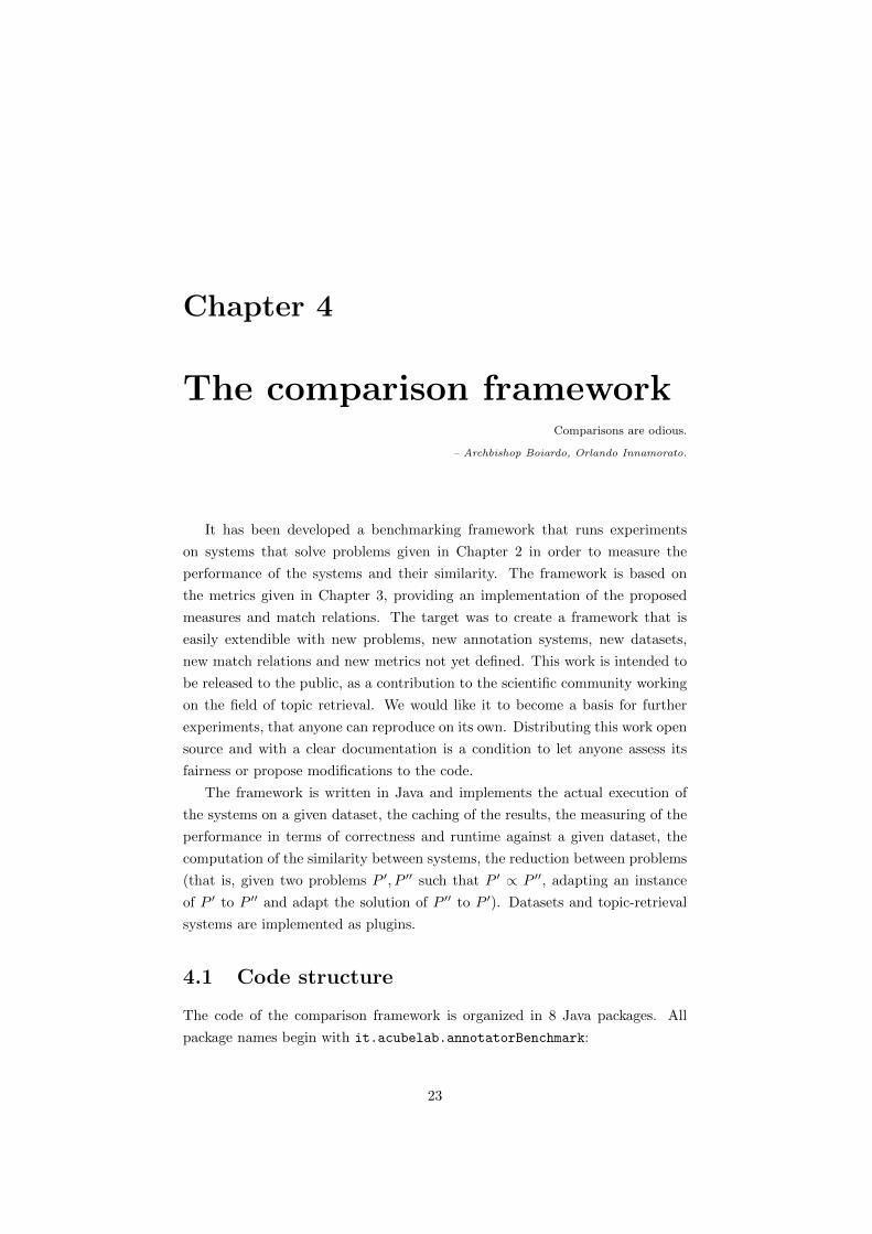
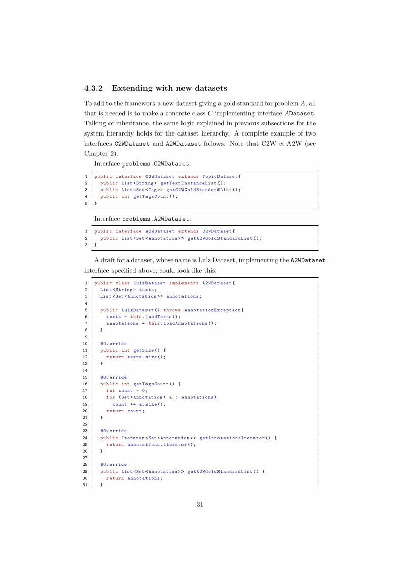
.problems contains interfaces representing a dataset for the problems defined in
Chapter 2 (such interfaces are called PDataset, where P is the name of the
problem, E.g. A2WDataset, C2WDataset) and the interfaces for a system
solving one of them (called PSystem, E.g. A2WSystem, C2WSystem)1. The
class hierarchy reflects the preordering of the problems given in Figure
2.2: if P ∝ Q then a system that solve Q can as well solve P . Speaking
of interfaces, this is reflected in the fact that a system that implements
interface QSystem (which defines a method for solving an instance of Q)
must also implement methods in PSystem (which defines a method for
solving an instance of P ), and thus QSystem extends PSystem. The
hierarchy of these classes is reported in Figure 4.2.
.datasetPlugins contains some implementations of PDataset interfaces of
package .problems. These classes provide standard datasets used in lit-
erature.
.systemPlugins contains some implementations of PSystem interfaces of pack-
age .problems, providing actual access to the topic-retrieval systems.
These classes are the glue between the benchmarking framework and the
topic-retrieval systems. Generally, in their implementation, to solve an
instance of a problem, they query the system through its web service or
running it locally.
.metrics contains the implementation of the metrics presented in Chapter 3.
The abstract class Metrics provides the methods for finding the true/false
positives/negatives and for computing precision, recall, F1 and similarity.
These methods need, as parameter, an object representing a match rela-
tion, like those given in Section 3.1. The implementations of the match
relations (StrongTagMatch, StrongAnnotationMatch, etc.) are as well
1Interfaces for problems for which there is no system (natively or not) solving it or datasetsgiving a gold standard for it, were not implemented in this version of the benchmarkingframework. They will be added if needed.
24
Figure 4.1: Automatically-generated UML class diagram with the packages ofthe annotator benchmark framework and their dependencies.
contained in this package. Classes representing a match relation on type
E implement the generic interface MatchRelation, using E as type param-
eter.
.utils contains some general-purpose utilities used along the whole frame-
work. This includes some Exceptions; some data-storing utilities; Export,
the utility to export a dataset in XML form; ProblemReduction that im-
plements the adaptations of instances and solutions needed for problem
reductions; and WikipediaApiInterface, that provides some methods to
query the Wikipedia API to retrieve information about concepts (Wikipe-
dia pages). In particular, WikipediaApiInterface.dereference(int)
implements the de-reference function d defined in Definition 4.
.scripts contains example scripts that run the benchmark on the datasets and
print data in gnuplot and LATEX style.
The packages form a kind of four-“layer” structure2, depicted in Figure 4.1.
At the two bottom layers lie the utility package and the data package, sparsely
used by all other packages. The third layer provides the abstract part of the
framework, including the interfaces and the implementation of the metrics mea-
surement. The fourth and most concrete layer provide both the caching and the
implementations of some datasets and systems.
2The layer term is abused, since packages in the upper layer may depend on all lowerlayers, and not only on the layer just below.
25
Figure 4.2: Hierarchy of interfaces that topic annotators must implement, re-flecting the hierarchy of the problems presented in 2.2.
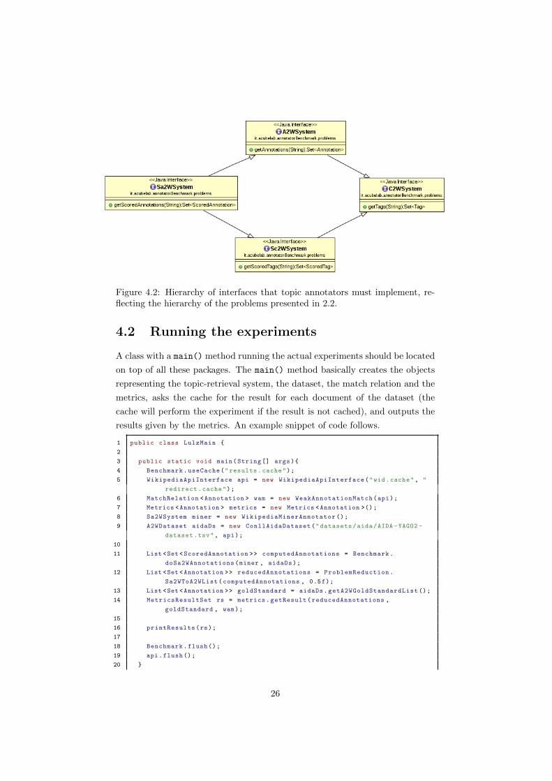
4.2 Running the experiments
A class with a main() method running the actual experiments should be located
on top of all these packages. The main() method basically creates the objects
representing the topic-retrieval system, the dataset, the match relation and the
metrics, asks the cache for the result for each document of the dataset (the
cache will perform the experiment if the result is not cached), and outputs the
results given by the metrics. An example snippet of code follows.
1 public class LulzMain {
2
3 public static void main(String [] args){
4 Benchmark.useCache("results.cache");
5 WikipediaApiInterface api = new WikipediaApiInterface("wid.cache", "
redirect.cache");
6 MatchRelation <Annotation > wam = new WeakAnnotationMatch(api);
7 Metrics <Annotation > metrics = new Metrics <Annotation >();
8 Sa2WSystem miner = new WikipediaMinerAnnotator ();
9 A2WDataset aidaDs = new ConllAidaDataset("datasets/aida/AIDA -YAGO2 -
dataset.tsv", api);
10
11 List <Set <ScoredAnnotation >> computedAnnotations = Benchmark.
doSa2WAnnotations(miner , aidaDs);
12 List <Set <Annotation >> reducedAnnotations = ProblemReduction.
Sa2WToA2WList(computedAnnotations , 0.5f);
13 List <Set <Annotation >> goldStandard = aidaDs.getA2WGoldStandardList ();
Figure 4.3: Main classes and interfaces involved in running the Wikipedia Minerannotator on the Conll/AIDA dataset. Both system and dataset will be pre-sented in Chapter 5
27
21
22 public static void printResults(MetricsResultSet rs){
23 // print the results
24 }
25 }
Let’s have a closer look at the snippet of code above. Figure 4.3 shows the
hierarchy of the classes and interfaces involved in this snippet. Lines 4-9 prepare
the environment: the cache containing the results of the problems is bound to
file results.cache. An object representing the API to Wikipedia is created
and assigned to variable api. This object is needed by the match method of
the WeakAnnotationMatch object, assigned to variable wam, that implements
the Weak annotation match: as defined in Definition 6, this match relation
is based on the dereference function, implemented by the Wikipedia API. An
object representing the Wikipedia Miner annotator – discussed in Chapter 5 –
is created and assigned to variable miner. In the implementation, this object
queries the Wikipedia Miner web service passing a document as parameter and
returning the resulting set of scored annotations. Furthermore, the dataset
AIDA/CoNLL is created, loading the instances (i.e. documents) and the gold
standard from a file.
Lines 11-14 call some methods to gather the actual output of the Wikipedia
Miner system for the dataset AIDA/CoNLL. If this system has already been
called for some of the text contained in the dataset, the result stored in the cache
will be quickly returned instead of calling the Wikipedia Miner web service.
Since Wikipedia Miner solve problem Sa2W, while the dataset represent a gold
standard for problem A2W, the output of Wikipedia Miner (for each document,
a set of scored annotations) must be adapted to the output of A2W, discarding
the scores and taking only the annotations above a given threshold. In the code
snippet, the adaption of the solution is done in line 12 and the threshold on the
score is set to 0.5. In line 14 the object representing the metrics is called, passing
as parameter the list of solutions adapted to A2W, the A2W gold standard given
by the dataset, and the Weak annotation match object. The metrics object
computes the actual measures like the true positives, the precision, the F1, etc.
Results are returned in an object of class MetricsResultSet whose content is
printed to the screen calling method printResults in line 16.
Lines 18-19 flush the cache of the results and of the Wikipedia API to a file
in a permanent memory, to guarantee a faster execution if the Main method is
executed twice.
28
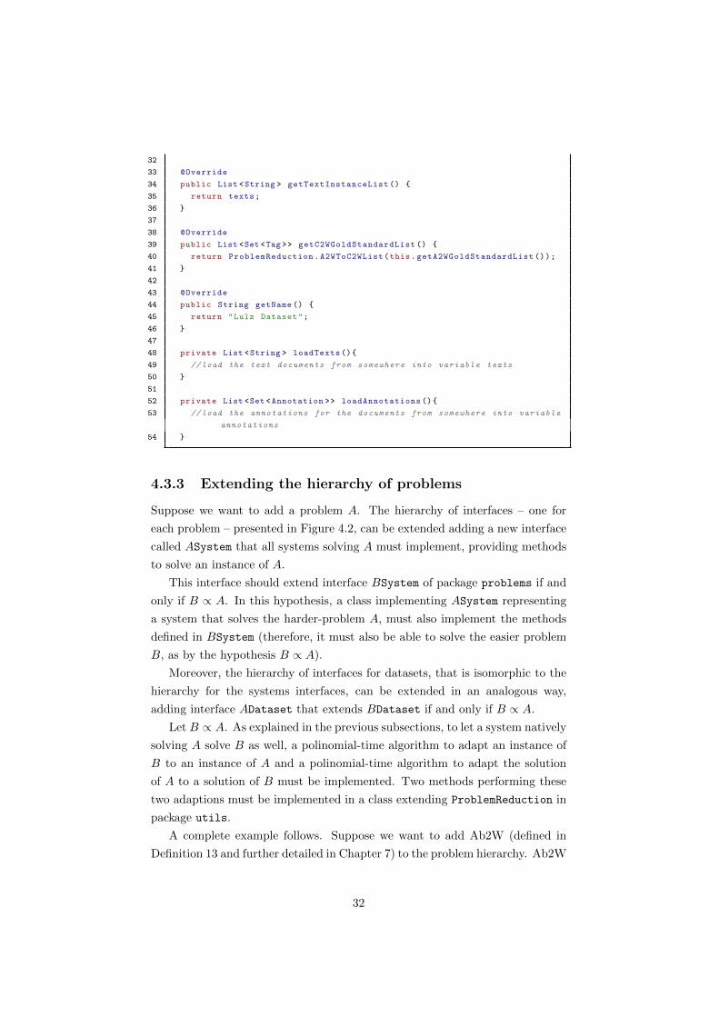
4.3 Extending the framework
An important feature of this benchmarking framework is that it can be easily
extended with new problems, new annotation systems, new datasets, new match
relations and new metrics. Let’s have a closer look at how an implementation
should be done for each of these categories.
4.3.1 Extending with new systems
To add to the framework a new system that solves a problem A, all that is
needed is to create a class that implements interface ASystem. Note that a
single system may natively solve more than one problem. In this case, the class
will implement one interface for each problem solved.
Suppose we want to add a new system called Cool Annotator that natively
solve A, and let B be a problem such that B ∝ A that Cool Annotator does not
natively solve. Let CoolAnnotator the concrete class representing the system,
implementing ASystem (and thus BSystem). CoolAnnotator will implement
a method defined in ASystem to solve problem A. The implementation of the
method defined in BSystem to solve problem B should simply
1. call routine methods to adapt the instance IB of problem B to an instance
IA of problem A. This takes polynomial time;
2. call the method defined in ASystem for solving problem A on the instance
IA, it will return solution SA;
3. adapt SA to a solution SB of problem B. This takes polynomial time;
4. return SB .
Methods for adapting the instances and the solutions from a problem to
another are implemented in the class ProblemReductions in package utils.
Here follows a complete example for A = A2W, B = T2W (thus, the reduction
is T2W ∝ A2W). The following interfaces are involved:
Interface problems.C2WSystem:
1 public interface C2WSystem extends TopicSystem {
2 public Set <Tag > solveC2W(String text) throws AnnotationException;
3 }
Interface problems.A2WSystem:
1 public interface A2WSystem extends C2WSystem{
2 public Set <Annotation > solveA2W(String text) throws AnnotationException
;
3 }
29
A draft for an annotator natively solving A2W (and thus solving C2W as
well), implementing the A2WSystem interface specified above, could look like
this:
1 public class CoolAnnotator implements A2WSystem{
2 private long lastTime = -1;
3
4 @Override
5 public Set <Annotation > solveA2W(String text) {
To introduce the extension of the metrics, we first have to explain how the
classes involved in the metrics measurement ineract with each other.
Package metrics contains class Metrics which implements the measures
defined in Chapter 3 (precision, recall, F1, etc). All methods for computing such
metrics take as argument a match relation M , implemented as an object of type
MatchRelation. For each match relation M given in Chapter 3, there is a class
implementing the interface MatchRelation that provides an implementation of
M in the method match.
Class Metrics is generic in that it has type variable T such that the measures
are computed over systems that return sets of objects of type T (E.g. T can be
Tag, Annotation, etc.). Therefore, measures like micro- and macro- F1, recall
and precision are performed for lists of sets of T-objects (a set for each instance
given by a dataset). Also interface MatchRelation has generic type variable
E, such that the match test is done on elements of type E. Of course, to use a
MatchRelation<E> with Metrics<T>, it must be T = E.
In other words, to assess the overall consistency, it must be true that:
34
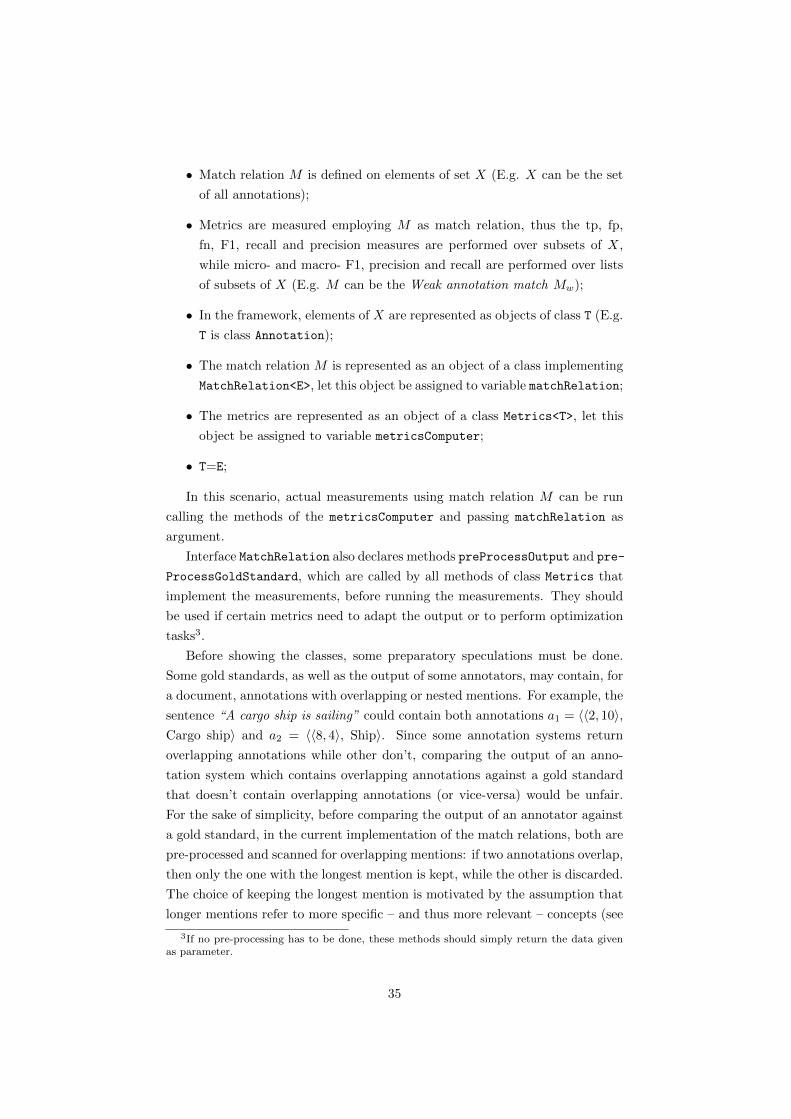
• Match relation M is defined on elements of set X (E.g. X can be the set
of all annotations);
• Metrics are measured employing M as match relation, thus the tp, fp,
fn, F1, recall and precision measures are performed over subsets of X,
while micro- and macro- F1, precision and recall are performed over lists
of subsets of X (E.g. M can be the Weak annotation match Mw);
• In the framework, elements of X are represented as objects of class T (E.g.
T is class Annotation);
• The match relation M is represented as an object of a class implementing
MatchRelation<E>, let this object be assigned to variable matchRelation;
• The metrics are represented as an object of a class Metrics<T>, let this
object be assigned to variable metricsComputer;
• T=E;
In this scenario, actual measurements using match relation M can be run
calling the methods of the metricsComputer and passing matchRelation as
argument.
Interface MatchRelation also declares methods preProcessOutput and pre-
ProcessGoldStandard, which are called by all methods of class Metrics that
implement the measurements, before running the measurements. They should
be used if certain metrics need to adapt the output or to perform optimization
tasks3.
Before showing the classes, some preparatory speculations must be done.
Some gold standards, as well as the output of some annotators, may contain, for
a document, annotations with overlapping or nested mentions. For example, the
sentence “A cargo ship is sailing” could contain both annotations a1 = 〈〈2, 10〉,Cargo ship〉 and a2 = 〈〈8, 4〉, Ship〉. Since some annotation systems return
overlapping annotations while other don’t, comparing the output of an anno-
tation system which contains overlapping annotations against a gold standard
that doesn’t contain overlapping annotations (or vice-versa) would be unfair.
For the sake of simplicity, before comparing the output of an annotator against
a gold standard, in the current implementation of the match relations, both are
pre-processed and scanned for overlapping mentions: if two annotations overlap,
then only the one with the longest mention is kept, while the other is discarded.
The choice of keeping the longest mention is motivated by the assumption that
longer mentions refer to more specific – and thus more relevant – concepts (see
3If no pre-processing has to be done, these methods should simply return the data givenas parameter.
35
the example of “Cargo ship” against “Ship”). Note that, using metrics based
on Weak annotation match, annotations with longer mentions are more likely
to result as a true positive.
Here follows the listing of (parts of) some classes involved in the extension
of the metrics.
Class metrics.Metrics implements the measures presented in Chapter 3:
1 public class Metrics <T> {
2
3 public MetricsResultSet getResult(List <Set <T>> outputOrig , List <Set <T>>
goldStandardOrig , MatchRelation <T> m) {
4 List <Set <T>> output = m.preProcessOutput(outputOrig);
5 List <Set <T>> goldStandard = m.preProcessGoldStandard(goldStandardOrig
5.2.1 Overview of the algorithmic features of the topic-
retrieval systems
The topic-retrieval systems, while addressing the same area of problems, exploit
different techniques.
TagMe searches the input text for mentions picked up by the set of Wikipedia
page titles, anchors and redirects. Each mention is associated to a set
of candidate concepts the mention may refer to. The disambiguation is
done exploiting the structure of the Wikipedia graph, trying to bind the
mentions to concepts that are related to each other, using the relatedness
measure [31] introduced in the Wikification algorithm, that takes into
account the amount of common in-going and outgoing links between the
two pages. TagMe disambiguation is enriched with a voting scheme, in
which all possible bindings between mentions and concepts express a vote
for the others, and the combination with highest vote average is selected.
Wikipedia Miner is an implementation of the Wikification algorithm pre-
sented in [33], one of the first approaches to the disambiguation to Wiki-
pedia. This system performs disambiguation before the identification of
mentions. Disambiguation is done with a machine-learning approach that
trains with links taken from Wikipedia pages (thus created by Wikipe-
dia users). Semantic relatedness between pages is not computed with the
relatedness measure of the original Wikification algorithm but is as well
machine-learned.
AIDA searches for mentions using the Stanford NER Tagger and uses the
YAGO2 knowledge base [16], which provides a catalog of concepts and the
relationships among concepts, including their semantic distance. AIDA
disambiguation comes in three variants:
PriorOnly Mentions are bound to the concept that is most commonly
bound in the knowledge base.
LocalDisambiguation Uses the local similarity disambiguation tech-
nique, that disambiguates each mention independently, without en-
forcing a semantic coherence among the mentions.
CocktailParty YAGO2 is used to perform a collective disambiguation of
the mentions: using a graph-based approach, the mapping between
mentions and concepts that preserves the highest coherence between
each other is iteratively found.
Illinois Wikifier as TagMe, the input text is searched for mentions extracted
by Wikipedia anchors and titles using the Illinois NER system [35]. The
42
Figure 5.1: Part of an example document (news story) given in the AIDA/-CoNLL dataset with its annotations, constituting the gold standard for thisdocument.
disambiguation problem is formulated as an optimization problem. As in
the other systems, a global approach is adopted, which instead of disam-
biguating each mention at a time, tries to disambiguate them all together,
preserving the highest coherence. Illinois Wikifier uses an original re-
latedness measure between Wikipedia pages based on NGD (Normalized
Google similarity distance) and PMI (Pointwise mutual information).
CMNS is meant to treat very short documents (e.g. Twitter posts). It gen-
erates a ranked list of candidate concepts for all N-grams in the input
text. The list is created through lexical matching and language modeling.
The disambiguation is done with a method based on supervised machine
learning that takes as input a set of documents and, for each document,
a set of annotations done by a human.
5.3 Available datasets
A noteworthy publication of a new system always comes along with test results
on peculiar datasets to assess its performance. Unfortunately, each system is
tested on different datasets and with different tricks and measures. Table 5.2
give a description for some of the published datasets, that were implemented in
the benchmarking framework.
Some extract of documents given by the datasets as instances, together with
the gold standard proposed by the dataset, are given in Figures 5.1, 5.2, 5.3,
5.4 and 5.5.
43
Dataset Description Publishedin
AIDA/CoNLL Contains a subset of the the original CoNLL 2003 entityrecognition task dataset. The documents are taken from theReuters Corpus V1 and consists of news stories. A quitelarge subset of mentions (though not all of them), includingthe most important ones, are annotated. Topics are anno-tated at each occurrence of a mention.
[17]
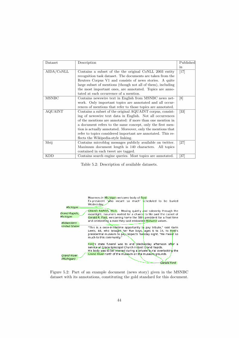
MSNBC Contains newswire text in English from MSNBC news net-work. Only important topics are annotated and all occur-rences of mentions that refer to those topics are annotated.
[8]
AQUAINT Contains a subset of the original AQUAINT corpus, consist-ing of newswire text data in English. Not all occurrencesof the mentions are annotated: if more than one mention ina document refers to the same concept, only the first men-tion is actually annotated. Moreover, only the mentions thatrefer to topics considered important are annotated. This re-flects the Wikipedia-style linking.
[33]
Meij Contains microblog messages publicly available on twitter.Maximum document length is 140 characters. All topicscontained in each tweet are tagged.
[27]
KDD Contains search engine queries. Most topics are annotated. [37]
Table 5.2: Description of available datasets.
Figure 5.2: Part of an example document (news story) given in the MSNBCdataset with its annotations, constituting the gold standard for this document.
44
Figure 5.3: Part of an example document (news story) given in the Aquaintdataset with its annotations, constituting the gold standard for this document.
Figure 5.4: Three example documents (twitter messages) given in the Meijdataset with their tags, constituting the gold standard for these documents.
Figure 5.5: Three example documents (search engine queries) given in the KDDdataset with their annotations, constituting the gold standard for these docu-ments.
45
Dataset NativeProblem
Docs Ann(Tags)
DistinctTopics
Avg.Ann/-Doc
Avg.length
Ann.fre-quency
AIDA/CO-NLL A2W 1393 27815 5591 20.0 1130 56−1
MSNBC A2W 20 658 279 32.9 3316 101−1
AQUAINT A2W 50 727 572 14.5 1415 98−1
Meij Rc2W 502 812 567 1.6 80 50−1
KDD A2W 1596 674 557 0.4 24 60−1
Table 5.3: Column Native Problem indicates the problem for which the datasetoffers a set of instances and their gold standard solutions. Docs is the numberof documents (instances) contained in the dataset. Ann (Tags) is the numberof overall annotations or tags in the dataset. Distinct Topics is the numberof distinct topics that appear in the dataset. Avg. Ann/Doc is the averagenumber of annotations or tags per document. Avg. length is the average lengthof a document in the dataset, in characters. Ann. frequency is the frequencyof annotations or tags per character (a value of n−1 indicates an average of oneannotation or tag every n characters).
Some datasets include annotations to concepts that no longer exist as pages
in the current version of Wikipedia. This may happen if a page have been
deleted or if its name was changed, and the dataset refers to an older version
of Wikipedia. In the implementation of the benchmarking system, annotations
with non-existing concepts are discarded.
Table 5.3 gives figures about the datasets. These figures help understanding
the nature of the datasets: AIDA/CO-NLL, MSNBC and AQUAINT address
about the same kind of documents (news stories written in good english and
good punctuation), the first being the most rich and complete, the others con-
taining longer documents (with less annotations). Meij is focused on twitter
messages (short text often with abbreviations and poor punctuation) and is
quite rich as well. KDD is focused on search engine queries (few keywords).
5.4 Comparing two systems for a given dataset
Figure 5.6 shows how two topic retrieval systems can be compared to each other
and the datasets they can be compared against. Keeping an eye at the graph,
the performance of systems S′ and S′′ in solving problem P can be compared
if and only if a reverse-path exists from problem P to system S′ and from
problem P to system S′′, and there is a dataset D representing a gold standard
for problem P ′|P ∝ P ′. In this case, the performance of systems S′ and S′′ can
be measured with respect to their ability to solve the instances of problem P
provided by dataset D. E.g.: The only way of comparing CMNS and Illinois
46
Illinois CMNS Wikipedia Miner AIDA
TagMe Sa2W*, Sc2W,A2W, Rc2W,D2W, C2W
Rc2W, C2W Sa2W*, Sc2W,A2W, Rc2W,D2W, C2W
Sa2W*, Sc2W,A2W, Rc2W,D2W, C2W
Illinois Rc2W, C2W Sa2W*, Sc2W,A2W, Rc2W,D2W, C2W
Sa2W*, Sc2W,A2W, Rc2W,D2W*, C2W
CMNS Rc2W, C2W Rc2W, C2W
WikipediaMiner
Sa2W*, Sc2W,A2W, Rc2W,D2W, C2W
Table 5.4: Comparability of the topic-retrieval systems for each problem. Prob-lems addressed natively by both systems are marked with a *.
Figure 5.6: Framing of the systems and datasets in the problem hierarchy. Eachsystem and each dataset is associated to the problem(s) it addresses natively.Systems are highlighted in pink, while datasets in yellow.
Wikifier is to compare their ability to solve problem C2W, and the comparison
can be done with respect to their ability to solve the instances provided by any
of the described datasets, since all of them can be adapted to give an instance
and a gold standard for the C2W problem, while Illinois Wikifier and TagMe
can be compared to each other for their ability to solve A2W, for example using
dataset AQUAINT.
The comparability between systems derived from the graph in Figure 5.6 is
presented in the matrix in Table 5.4.
5.5 Conclusions
In this chapter, we presented some of the publicly available systems, selected for
their originality, that solve problems related to topic retrieval. For each systems,
the problem(s) natively solved is reported, together with its main features. Since
the reviewed systems are all based upon Wikipedia as a knowledge basis, we
47
briefly presented some features of this online encyclopedia.
Some publicly available datasets, representing a set of instances and a gold
standard for some problems, have been reviewed, together with their main fea-
tures. These datasets can be used to perform experiments and check the ability
of a system in solving the problems for the instances given by the dataset.
48
Chapter 6
Experimental ResultsE quindi uscimmo a riveder le stelle.
– Dante Alighieri, La Divina Commedia, Canto XXXIV
Let’s put all the pieces together: in this chapter, benchmarking results given
by the framework illustrated in Chapter 4 are presented and commented. Ex-
periments were run benchmarking the topic retrieval systems with the datasets
presented in Chapter 5. The measures of performance and similarity are those
proposed in Chapter 3. Problems presented in Chapter 2 and their reductions
are the underlying basis for the analysis.
6.1 Setting up the experiments
6.1.1 Employed software and APIs
The benchmark has been done using the most up-to-date APIs or software made
available by their authors. TagMe has been tested using the publicly available
APIs [3] in September 2012; experiments on AIDA have been performed using
the AIDA RMI Service updated on 30/07/2012 [1]; experiments on Wikipe-
dia Miner have been performed querying the API publicly available at [4] in
September 2012; Illinois Wikifier has been downloaded from [2] in August 2012
and run locally.
6.1.2 Performed experiments
Three experiments, each exploring the ability of the systems on certian kinds
of datasets, have been set up. Configurations for the experiments are given in
Table 6.1.
49
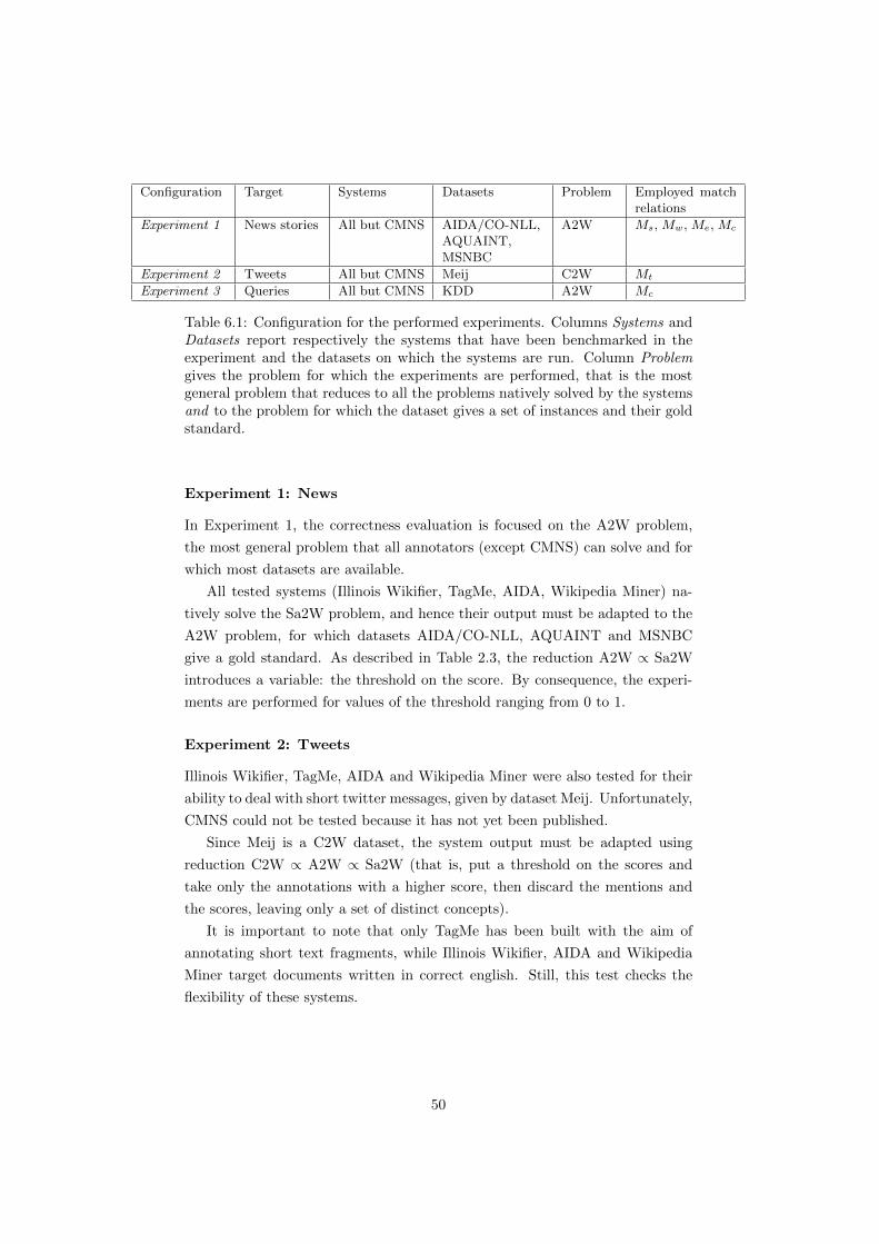
Configuration Target Systems Datasets Problem Employed matchrelations
Experiment 1 News stories All but CMNS AIDA/CO-NLL,AQUAINT,MSNBC
A2W Ms, Mw, Me, Mc
Experiment 2 Tweets All but CMNS Meij C2W Mt
Experiment 3 Queries All but CMNS KDD A2W Mc
Table 6.1: Configuration for the performed experiments. Columns Systems andDatasets report respectively the systems that have been benchmarked in theexperiment and the datasets on which the systems are run. Column Problemgives the problem for which the experiments are performed, that is the mostgeneral problem that reduces to all the problems natively solved by the systemsand to the problem for which the dataset gives a set of instances and their goldstandard.
Experiment 1: News
In Experiment 1, the correctness evaluation is focused on the A2W problem,
the most general problem that all annotators (except CMNS) can solve and for
which most datasets are available.
All tested systems (Illinois Wikifier, TagMe, AIDA, Wikipedia Miner) na-
tively solve the Sa2W problem, and hence their output must be adapted to the
A2W problem, for which datasets AIDA/CO-NLL, AQUAINT and MSNBC
give a gold standard. As described in Table 2.3, the reduction A2W ∝ Sa2W
introduces a variable: the threshold on the score. By consequence, the experi-
ments are performed for values of the threshold ranging from 0 to 1.
Experiment 2: Tweets
Illinois Wikifier, TagMe, AIDA and Wikipedia Miner were also tested for their
ability to deal with short twitter messages, given by dataset Meij. Unfortunately,
CMNS could not be tested because it has not yet been published.
Since Meij is a C2W dataset, the system output must be adapted using
reduction C2W ∝ A2W ∝ Sa2W (that is, put a threshold on the scores and
take only the annotations with a higher score, then discard the mentions and
the scores, leaving only a set of distinct concepts).
It is important to note that only TagMe has been built with the aim of
annotating short text fragments, while Illinois Wikifier, AIDA and Wikipedia
Miner target documents written in correct english. Still, this test checks the
flexibility of these systems.
50
Experiment 3: Search engine queries (a preliminary study)
KDD dataset containing search engine queries is for problem A2W, and can
be given as input to Illinois Wikifier, TagMe, AIDA and Wikipedia Miner.
Nonetheless, in this case, we are not interested in computing annotations, but
only in concepts. That’s why the only match function adopted is the Concept
annotation match defined in Definition 8.
In this case, none of the systems were designed to address this kind of doc-
uments, made only of keywords. To work on this dataset, major modifications
should be applied to the reviewed systems. A study more focused on this task is
presented in [19]. For systems are used as they come, the results are extremely
poor, though showing some interesting results about their flexibility.
6.2 Results for Experiment 1: news
6.2.1 Finding the annotations
Note that each of the Sa2W annotators give a different meaning to the score, so
it does not make sense to compare the performance of two annotators for the
same threshold. The question that can instead be answered is: If an annotator
knew its optimal threshold on the score, which annotator would perform best?
To answer this question, the metrics presented in Chapter 3 have been
measured. The interesting data is the maximum value of F1micro(Rt, G,Mw)
reached varying the threshold t, where Mw is the Weak annotation match, G is
the gold standard, Rt is the result of the system adapted as an output of the
A2W problem using t as threshold. This measure for the tagging systems is
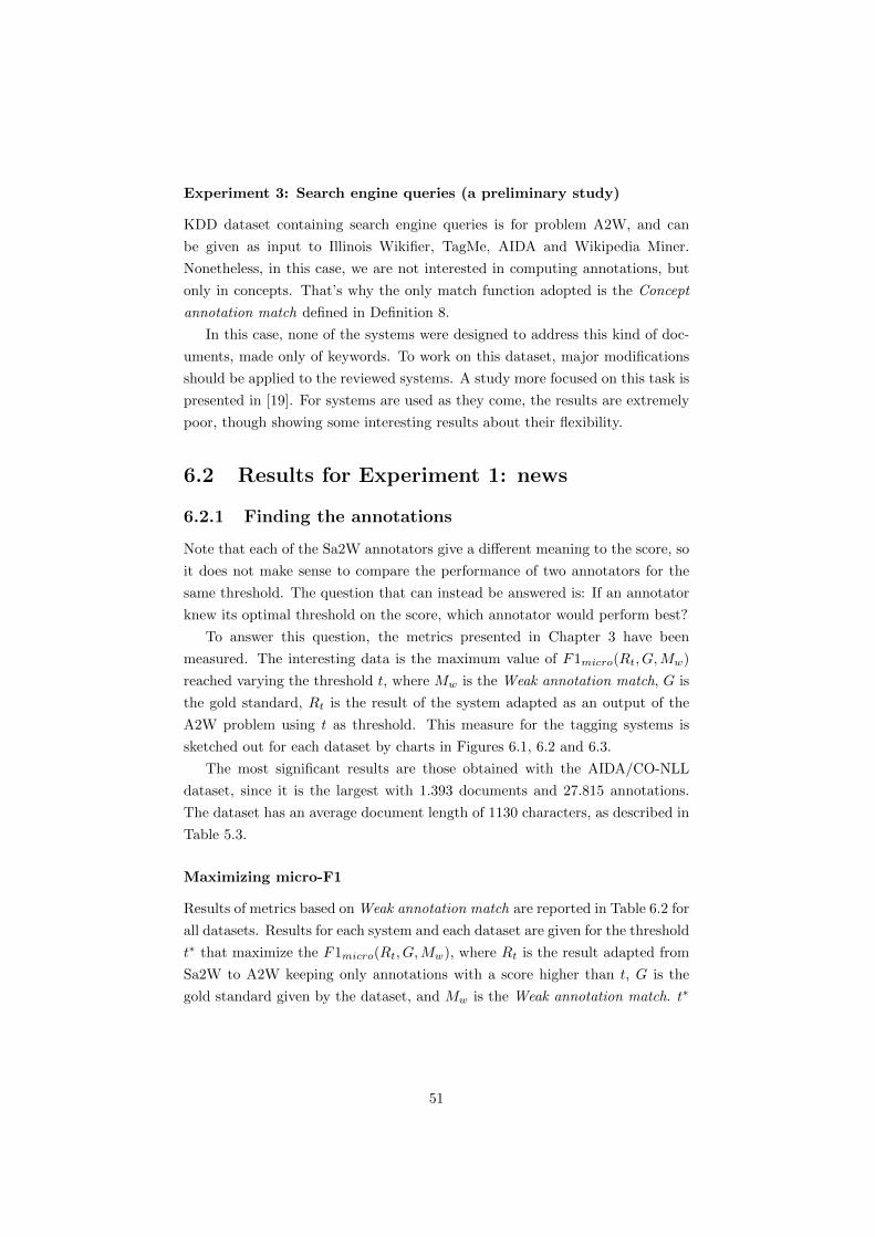
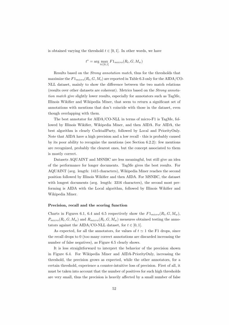
sketched out for each dataset by charts in Figures 6.1, 6.2 and 6.3.
The most significant results are those obtained with the AIDA/CO-NLL
dataset, since it is the largest with 1.393 documents and 27.815 annotations.
The dataset has an average document length of 1130 characters, as described in
Table 5.3.
Maximizing micro-F1
Results of metrics based on Weak annotation match are reported in Table 6.2 for
all datasets. Results for each system and each dataset are given for the threshold
t∗ that maximize the F1micro(Rt, G,Mw), where Rt is the result adapted from
Sa2W to A2W keeping only annotations with a score higher than t, G is the
gold standard given by the dataset, and Mw is the Weak annotation match. t∗
51
is obtained varying the threshold t ∈ [0, 1]. In other words, we have
t∗ = arg maxt∈[0,1]
F1micro(Rt, G,Mw)
Results based on the Strong annotation match, thus for the thresholds that
maximize the F1micro(Rt, G,Ms) are reported in Table 6.3 only for the AIDA/CO-
NLL dataset, mainly to show the difference between the two match relations
(results over other datasets are coherent). Metrics based on the Strong annota-
tion match give slightly lower results, especially for annotators such as TagMe,
Illinois Wikifier and Wikipedia Miner, that seem to return a significant set of
annotations with mentions that don’t coincide with those in the dataset, even
though overlapping with them.
The best annotator for AIDA/CO-NLL in terms of micro-F1 is TagMe, fol-
lowed by Illinois Wikifier, Wikipedia Miner, and then AIDA. For AIDA, the
best algorithm is clearly CocktailParty, followed by Local and PriorityOnly.
Note that AIDA have a high precision and a low recall - this is probably caused
by its poor ability to recognize the mentions (see Section 6.2.2): few mentions
are recognized, probably the clearest ones, but the concept associated to them
is mostly correct.
Datasets AQUAINT and MSNBC are less meaningful, but still give an idea
of the performance for longer documents. TagMe gives the best results. For
AQUAINT (avg. length: 1415 characters), Wikipedia Miner reaches the second
position followed by Illinois Wikifier and then AIDA. For MSNBC, the dataset
with longest documents (avg. length: 3316 characters), the second most per-
forming is AIDA with the Local algorithm, followed by Illinois Wikifier and
Wikipedia Miner.
Precision, recall and the scoring function
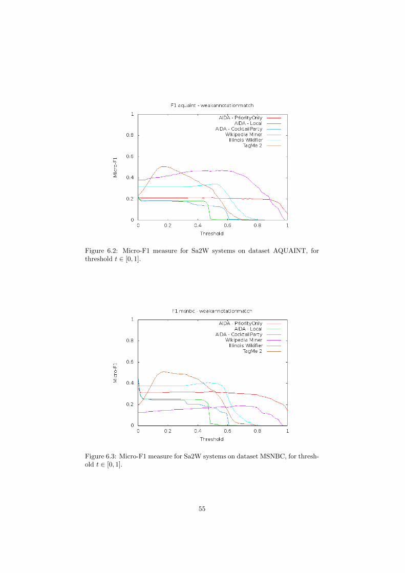
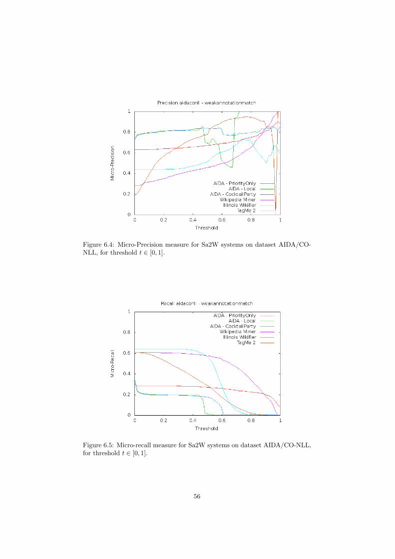
Charts in Figures 6.1, 6.4 and 6.5 respectively show the F1micro(Rt, G,Mw),
Pmicro(Rt, G,Mw) and Rmicro(Rt, G,Mw) measures obtained testing the anno-
tators against the AIDA/CO-NLL dataset, for t ∈ [0, 1].
As expected, for all the annotators, for values of t ' 1 the F1 drops, since
the recall drops to 0 (too many correct annotations are discarded increasing the
number of false negatives), as Figure 6.5 clearly shows.
It is less straightforward to interpret the behavior of the precision shown
in Figure 6.4. For Wikipedia Miner and AIDA-PriorityOnly, increasing the
threshold, the precision grows as expected, while the other annotators, for a
certain threshold, experience a counter-intuitive loss of precision. First of all, it
must be taken into account that the number of positives for such high thresholds
are very small, thus the precision is heavily affected by a small number of false
Wikipedia Miner 0.594 0.520 0.495 0.547 15227 15537 12587
Table 6.2: The main results about correctness is shown in this table.Column F1micro indicates the maximum micro-F1 measure computed asF1micro(Rt∗ , G,Mw), where t∗ is the threshold that maximizes the micro-F1.Column Best Threshold indicates t∗. Columns Pmicro and Rmicro indicate themicro-precision and micro-recall for the same threshold t∗. Columns tp, fp, fnrespectively show the overall true positives, false positives and false negativesfor the results of the dataset, still for threshold t∗.
Wikipedia Miner 0.594 0.474 0.413 0.556 15472 22034 12343
Table 6.3: Results based on Strong annotation match (Only for AIDA/CONLLdataset). Column F1micro indicates the maximum micro-F1 measure computedas F1micro(Rt∗ , G,Ms). For a description of the other columns, see Table 6.2.
53
Figure 6.1: Micro-F1 measure for Sa2W systems on dataset AIDA/CO-NLL,for threshold t ∈ [0, 1].
positives. Anyhow, this behavior demonstrates that a certain number of wrong
annotations have a high score. Note that this behavior does not have a big
influence on the F1 measure, since for these thresholds the recall is very close
to 0, and so is the F1.
The behaviour of the precision and recall in Figures 6.4 and 6.5 give an
evidence of the performance of an important feature of an annotation system.
As said in the introduction of Chapter 3, one factor which the performance of
a system depends upon how good the system is in assigning the score to the
annotations. This issue should be inspected more in-depth, but some assump-
tions can be made: Let p(a) be the probability that annotation a is correct, and
let s(a) be the scoring function. The ideal scoring function is s∗(a) = p(a). A
good scoring function should obviously assign higher scores to annotations that
are more likely to be correct, thus it should be s(a′) ≥ s(a′′) ⇔ p(a′) ≥ p(a′′).
In this scenario, functions describing precision and recall would be respectively
monotonically non-decreasing and monotonically non-increasing.
While for the recall chart in Figure 6.5 this property seems to be respected,
the precision chart given in Figure 6.4 indicates a failure for the scoring functions
of AIDA-Local, AIDA-CockailParty, Illinois Wikifier and TagMe, that, in some
cases, assign a high score to wrong annotations, while the scoring functions of
Wikipedia Miner and AIDA-PriorityOnly seem to perform better.
54
Figure 6.2: Micro-F1 measure for Sa2W systems on dataset AQUAINT, forthreshold t ∈ [0, 1].
Figure 6.3: Micro-F1 measure for Sa2W systems on dataset MSNBC, for thresh-old t ∈ [0, 1].
55
Figure 6.4: Micro-Precision measure for Sa2W systems on dataset AIDA/CO-NLL, for threshold t ∈ [0, 1].
Figure 6.5: Micro-recall measure for Sa2W systems on dataset AIDA/CO-NLL,for threshold t ∈ [0, 1].
Wikipedia Miner 0.484 0.682 0.607 0.779 21610 13976 6139
Table 6.4: Results based on Mention annotation match (Only for AIDA/CONLLdataset). Column F1micro indicates the maximum micro-F1 measure computedas F1micro(Rt∗ , G,Mm). For a description of the other columns, see Table 6.2.
6.2.2 Finding the mentions
As illustrated in Section 3.2, the sub-task of finding the mentions can be mea-
sured using the same micro-F1, micro-recall and micro-precision measures com-
bined with the Mention annotation match relation M = Mm.
The value of F1micro(Rt∗ , G,Mm) (for the threshold t∗ that maximizes it)
for the experiment ran on the AIDA/CO-NLL dataset is given for each system
in Table 6.4 and basically shows the performance of the NER algorithms used
by the annotation systems. Methods of the AIDA system use the same NER
system (Stanford NER tagger) and obviously have the same result, that is the
lowest one in terms of F1 but provides a very high precision. Illinois Wikifier
(that uses the Illinois Named Entity Tagger) shows similar results to Wikipedia
Miner. TagMe has a higher precision but a lower recall.
6.2.3 Finding the concepts
Keeping in mind Section 3.3, the sub-task of finding the concepts can be mea-
sured with the same metrics used in the other tests, combined with the Concept
annotation match M = Mc.
The value of F1micro(Rt∗ , G,Mc) (for the threshold t∗ that maximizes it) for
the experiment ran on the AIDA/CO-NLL dataset is given for each system in
Table 6.5. TagMe outperforms the other annotators in terms of F1 and recall,
while the highest precision is achieved by AIDA-CocktailParty, that has a very
low recall. The CocktailParty algorithm seems to be the best in the choice of
the AIDA algorithms, being slightly better than Local and significantly better
Wikipedia Miner 0.594 0.532 0.489 0.582 9708 10132 6962
Table 6.5: Results based on Concept annotation match (Only for AIDA/CONLLdataset). Column F1micro indicates the maximum micro-F1 measure computedas F1micro(Rt∗ , G,Mc). For a description of the other columns, see Table 6.2.
6.2.4 Output similarity
As described in Section 3.4, the outputs of two annotators can be compared to
understand how similar they are. This is measured with the Smicro and Smacro
measures given in Definition 10, combined with any match relation, depending
on what we want to check the similarity of, as described in Subsection 3.4.3.
Similarity of the annotations
In Table 6.6 are reported values of the similarity measure Smacro(At′ , Bt′′ ,Mw)
defined in Definition 10, where A and B are the output of each pair of annotators
and At′ and Bt′′ are the output keeping only annotations with a score above the
thresholds that maximize the micro-F1 (those reported in Table 6.2). These sets
include true positives and false positives found by the tagging systems. As match
relation M , the Weak annotation match Mw has been used. In other words, the
Smacro(At′ , Bt′′ ,Mw) measure given in Table 6.6 represents the similarity of the
best output of two systems, including both true and false positives.
As said in Subsection 3.4.4, the fraction of true positives can be measured
in detail. Table 6.7 is analogous to Table 6.6 except that the similarity
Smacro(T (At′ , G,Mw), T (Bt′′ , G,Mw),Mw)
is not computed on the whole output, but is restricted to the true positives
using the T function defined in Definition 11. Hence, this measure shows how
many of the correct annotations two systems have in common.
As expected, the highest similarities are between the methods of the AIDA
system, that all use the same NER algorithm. A similarity around 50% is also
shown between Illinois Wikifier, Wikipedia Miner and TagMe, while these three
58
TagMe 2 IllinoisWikifier
AIDA-Local
AIDA-CocktailParty
AIDA-PriorityOnly
WikipediaMiner
TagMe 2 1.000 0.407 0.325 0.318 0.342 0.533
Illinois Wiki-fier
1.000 0.246 0.245 0.240 0.545
AIDA-Local 1.000 0.921 0.821 0.306
AIDA-CocktailParty
1.000 0.808 0.300
AIDA-PriorityOnly
1.000 0.317
WikipediaMiner
1.000
Table 6.6: Similarity between the annotation systems, given as the Smacro mea-sure on the best outputs for the AIDA/CONLL dataset.
TagMe 2 IllinoisWikifier
AIDA-Local
AIDA-CocktailParty
AIDA-PriorityOnly
WikipediaMiner
TagMe 2 1.000 0.600 0.444 0.435 0.463 0.686
Illinois Wiki-fier
1.000 0.430 0.427 0.431 0.691
AIDA-Local 1.000 0.963 0.899 0.471
AIDA-CocktailParty
1.000 0.884 0.464
AIDA-PriorityOnly
1.000 0.490
WikipediaMiner
1.000
Table 6.7: Similarity between the annotation systems, given as the Smacro mea-sure on the true positives of the best outputs for the AIDA/CONLL dataset.
systems are rather dissimilar to the AIDA system. Results in Table 6.7 enhances
those in Table 6.6.
Similarity of the mentions
To check the similarity of the systems in recognizing the mentions, the same S
measure has been computed using M = Mm, that is, the Mention annotation
match is used as match relation. Here, the measure
Smacro(T (At′ , G,Mm), T (Bt′′ , G,Mm),Mm)
represents how much of the correct output have overlapping annotations. At′
and Bt′′ are selected using the thresholds reported in Table 6.4, that maximize
the recognition of mentions. Moreover, At′ and Bt′′ are restricted to the true
59
TagMe 2 IllinoisWikifier
AIDA-Local
AIDA-CocktailParty
AIDA-PriorityOnly
WikipediaMiner
TagMe 2 1.000 0.700 0.498 0.498 0.498 0.754
Illinois Wiki-fier
1.000 0.503 0.502 0.503 0.819
AIDA-Local 1.000 0.999 1.000 0.545
AIDA-CocktailParty
1.000 0.999 0.545
AIDA-PriorityOnly
1.000 0.545
WikipediaMiner
1.000
Table 6.8: Similarity between the annotation systems in recognizing the men-tions, given as the Smacro measure on the outputs that maximize the F1 for therecognition of mentions. Results for the AIDA/CONLL dataset.
positives using the T function defined in Definition 11.
Results are shown in Table 6.8. The mention recognition for the AIDA
algorithm is the same, and thus show a similarity of 1. Wikipedia Miner shares
around 75% of mentions with TagMe and Illinois Wikifier, while AIDA have only
about 50% of mentions in common with the other systems. These data seem
to indicate that a big part of the performance of a system in solving problem
Sa2W and A2W is determined by the way mentions are recognized in the text.
Similarity of the concepts
The similarity for the concepts,
Smacro(T (At′ , G,Mm), T (Bt′′ , G,Mm),Mm)
is reported in Table 6.9. At′ and Bt′′ are selected using the thresholds reported
in Table 6.4, that maximize the recognition of concepts. Moreover, At′ and Bt′′
are restricted to the true positives using the T function defined in Definition 11.
Hence, values reported in Table 6.9 show how many of the correct concepts are
in common between two systems.
The similarity between the AIDA algorithms is still the highest, and all sim-
ilarities are above 50%, indicating that more than half of the retrieved concepts
are in common. A rather high similarity is shown between Wikipedia Miner,
TagMe and Illinois Wikifier.
60
TagMe 2 IllinoisWikifier
AIDA-Local
AIDA-CocktailParty
AIDA-PriorityOnly
WikipediaMiner
TagMe 2 1.000 0.675 0.526 0.525 0.525 0.750
Illinois Wiki-fier
1.000 0.541 0.542 0.534 0.720
AIDA-Local 1.000 0.968 0.918 0.569
AIDA-CocktailParty
1.000 0.904 0.564
AIDA-PriorityOnly
1.000 0.580
WikipediaMiner
1.000
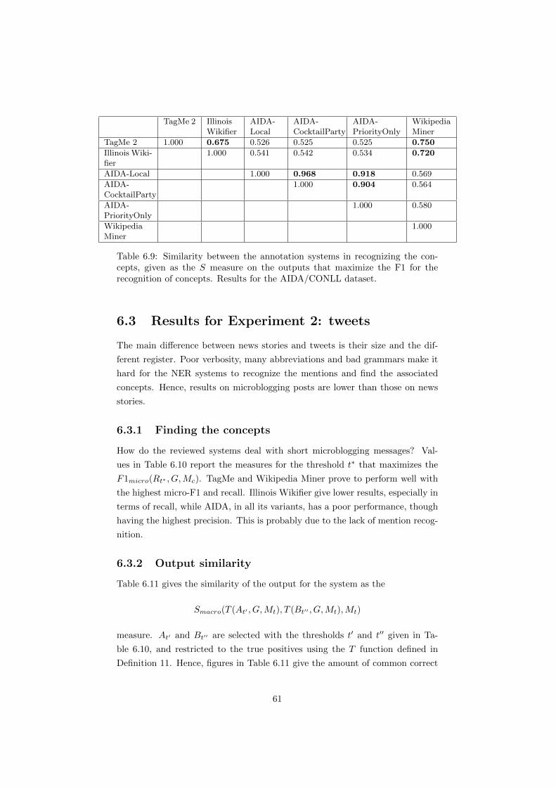
Table 6.9: Similarity between the annotation systems in recognizing the con-cepts, given as the S measure on the outputs that maximize the F1 for therecognition of concepts. Results for the AIDA/CONLL dataset.
6.3 Results for Experiment 2: tweets
The main difference between news stories and tweets is their size and the dif-
ferent register. Poor verbosity, many abbreviations and bad grammars make it
hard for the NER systems to recognize the mentions and find the associated
concepts. Hence, results on microblogging posts are lower than those on news
stories.
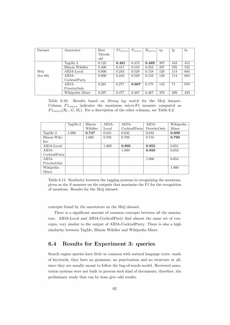
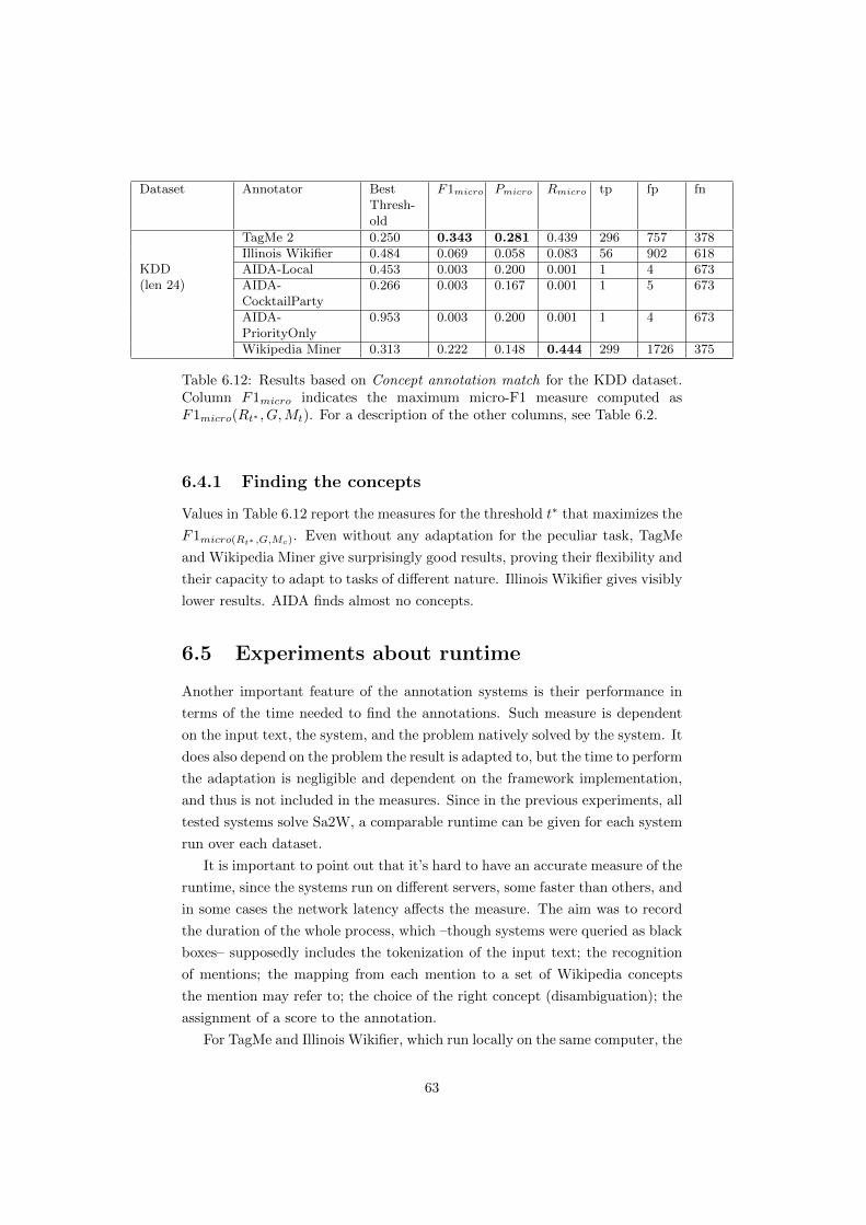
6.3.1 Finding the concepts
How do the reviewed systems deal with short microblogging messages? Val-
ues in Table 6.10 report the measures for the threshold t∗ that maximizes the
F1micro(Rt∗ , G,Mc). TagMe and Wikipedia Miner prove to perform well with
the highest micro-F1 and recall. Illinois Wikifier give lower results, especially in
terms of recall, while AIDA, in all its variants, has a poor performance, though
having the highest precision. This is probably due to the lack of mention recog-
nition.
6.3.2 Output similarity
Table 6.11 gives the similarity of the output for the system as the
Smacro(T (At′ , G,Mt), T (Bt′′ , G,Mt),Mt)
measure. At′ and Bt′′ are selected with the thresholds t′ and t′′ given in Ta-
ble 6.10, and restricted to the true positives using the T function defined in
Definition 11. Hence, figures in Table 6.11 give the amount of common correct
Wikipedia Miner 0.297 0.477 0.487 0.467 379 399 433
Table 6.10: Results based on Strong tag match for the Meij dataset.Column F1micro indicates the maximum micro-F1 measure computed asF1micro(Rt∗ , G,Mt). For a description of the other columns, see Table 6.2.
TagMe 2 IllinoisWikifier
AIDA-Local
AIDA-CocktailParty
AIDA-PriorityOnly
WikipediaMiner
TagMe 2 1.000 0.747 0.631 0.635 0.632 0.809
Illinois Wiki-fier
1.000 0.705 0.709 0.716 0.790
AIDA-Local 1.000 0.995 0.955 0.651
AIDA-CocktailParty
1.000 0.959 0.653
AIDA-PriorityOnly
1.000 0.654
WikipediaMiner
1.000
Table 6.11: Similarity between the tagging systems in recognizing the mentions,given as the S measure on the outputs that maximize the F1 for the recognitionof mentions. Results for the Meij dataset.
concepts found by the annotators on the Meij dataset.
There is a significant amount of common concepts between all the annota-
tors. AIDA-Local and AIDA-CocktailParty find almost the same set of con-
cepts, very similar to the output of AIDA-CocktailParty. There is also a high
similarity between TagMe, Illinois Wikifier and Wikipedia Miner.
6.4 Results for Experiment 3: queries
Search engine queries have little in common with natural language texts: made
of keywords, they have no grammar, no punctuation and no structure at all,
since they are usually meant to follow the bag-of-words model. Reviewed anno-
tation systems were not built to process such kind of documents, therefore, the
preliminary study that can be done give odd results.
Wikipedia Miner 0.313 0.222 0.148 0.444 299 1726 375
Table 6.12: Results based on Concept annotation match for the KDD dataset.Column F1micro indicates the maximum micro-F1 measure computed asF1micro(Rt∗ , G,Mt). For a description of the other columns, see Table 6.2.
6.4.1 Finding the concepts
Values in Table 6.12 report the measures for the threshold t∗ that maximizes the
F1micro(Rt∗ ,G,Mc). Even without any adaptation for the peculiar task, TagMe
and Wikipedia Miner give surprisingly good results, proving their flexibility and
their capacity to adapt to tasks of different nature. Illinois Wikifier gives visibly
lower results. AIDA finds almost no concepts.
6.5 Experiments about runtime
Another important feature of the annotation systems is their performance in
terms of the time needed to find the annotations. Such measure is dependent
on the input text, the system, and the problem natively solved by the system. It
does also depend on the problem the result is adapted to, but the time to perform
the adaptation is negligible and dependent on the framework implementation,
and thus is not included in the measures. Since in the previous experiments, all
tested systems solve Sa2W, a comparable runtime can be given for each system
run over each dataset.
It is important to point out that it’s hard to have an accurate measure of the
runtime, since the systems run on different servers, some faster than others, and
in some cases the network latency affects the measure. The aim was to record
the duration of the whole process, which –though systems were queried as black
boxes– supposedly includes the tokenization of the input text; the recognition
of mentions; the mapping from each mention to a set of Wikipedia concepts
the mention may refer to; the choice of the right concept (disambiguation); the
assignment of a score to the annotation.
For TagMe and Illinois Wikifier, which run locally on the same computer, the
Table 6.13: The average time needed by the annotation systems to annotate thedocuments contained in the datasets. In the first column, the average length ofthe documents contained in the dataset is reported.
runtime has been recorded as the difference between the system time after and
before the library call; For AIDA, the time has been recorded as that returned
by the method getOverallRuntime() of the RMI Service, and thus does not
include network latency; For Wikipedia Miner, that is accessed through a web
service, the time has been recorded as the difference between the system time
after and before the query, and the timing has been calibrated subtracting the
time needed to process an empty query.
Despite the heterogeneity and roughness of the methods used to record the
timings, the figures differ enough to give a meaningful idea of how fast the
annotation systems work. Data for each system and dataset is given in Table
6.13.
Results show that TagMe and Wikipedia Miner have similar runtime per-
64
Figure 6.6: Average runtime (in log-scale) for dataset AIDA/CO-NLL and bestachieved F1 measures (metrics based on Weak annotation match).
formance, suggesting their deployment in large-scale data processing. Illinois
Wikifier is about 3 times slower. AIDA with PriorityOnly algorithm is the
fastest one (this is due to the trivial disambiguation process) while the other
methods, Local and CocktailParty are way slower, with the first being about 10
times and the latter being 30 times slower than TagMe and Wikipedia Miner.
For all of them, the time needed to find the annotations looks linear in the size
of the text – which is good. Chart in Figure 6.6 compares the runtime and
the achieved best F1 measure for the systems when performing tests on the
AIDA/CO-NLL dataset.
6.6 Conclusions
This chapter have reported the results given by the benchmarking framework
applied on the systems and datasets presented in the previous chapters. Three
experiments were run, each focusing on a different kinds of datasets: the news
stories, the twitter messages and the search engine queries. Commenting the
results, we highlighted some features and some weaknesses of the systems.
All systems can be improved but, at least for news and tweets, results are
encouraging. TagMe seems to outperform the other systems in each of the three
experiments, though other systems show interesting results. AIDA seems to
have a main weakness in the recognition of mentions.
65
For the queries, all systems clearly need a major adaptation. TagMe and
Wikipedia Miner incredibly give meaningful results even on this kind of dataset.
Despite not being satisfactory, results encourage the application of these systems
on search engine queries.
The similarity of the system outputs have also been measured, showing a
rather high similarity between TagMe, Illinois Wikifier and Wikipedia Miner,
while AIDA seem to find rather distinct annotations.
The measured runtime show the fundamental property that the time needed
to annotate a document is linear in the size of the document. This makes it
possible, especially for faster systems like TagMe, Wikipedia Miner and Illinois
Wikifier, to apply them to large-scale datasets.
66
Chapter 7
Future DevelopmentsGutta cavat lapidem non vi, sed saepe cadendo
– Latin proverb.
This thesis gives a contribution to a line of research that is moving its first
steps of development, and forecasting its future advancement is a hard job of
imagination. Though, some lines of expansion can be sketched out. First of
all, new algorithms and systems can be developed to enhance the performance
in solving the topic-retrieval problems. Moreover, the benchmark needs a clear
documentation provided in Javadoc that has not yet been done, and will prob-
ably need to be maintained reflecting the state of the art measures, even fixing
the bugs its code certainly hides. On the theoretical side, the measures pre-
sented in Chapter 3 can be expanded to inspect certain aspects of a system
performance.
7.1 Definition of new problems
The problems defined in Chapter 2 are not the only problems related to topic
retrieval. New problems can be formulated, exploring new horizons for this
research area.
7.1.1 Assigning a relevance to a topic
Most of the systems presented in Chapter 5 assign to the annotations a likelihood
score, expressing the probability that the annotation is correct, but none of them
deal with the task of finding the relevance of the topics, i.e. how important the
topic is to describe the content of the input text. This information would be
crucial to assist text categorization, text clustering and the document retrieval.
67
Figure 7.1: Examples of instances of the Ab2W and RelA2W problems andtheir correct solution. Scored tags are highlighted in blue, scored annotationsin green. Concepts are in italics.
Definition 12 Relevance scored annotations to Wikipedia (Rsa2W) is the prob-
lem of identifying the set of annotations in a text and assign them both a
likelihood score s and a relevance score r indicating how relevant the topic is
to describe the contents of the text. The solution consists of a set of tuples
〈m, c, s, r〉 where m is the mention (a pair (p, l) where p is the index of the
character where the mention begin and l is the length of the mention), c is
the concept, s is the likelihood score and r is a real number r ∈ R, r ∈ [0, 1]
indicating the relevance of the concept to describe the topics of the input text.
An example instance of this problem and its solution is given in Figure 7.1.
7.1.2 Finding relevant non-mentioned topics
Another natural expansion of the problems presented in Chapter 2 can be the
definition of a new problem, Ab2W.
Definition 13 Abstraction to Wikipedia (Ab2W) is the problem of identifying
the set of concepts that are mentioned in the input text, assigning them both a
relevance score and a likelihood score, plus the concepts the text expresses, even
though they are not mentioned in the text (i.e. they are implicitly expressed).
A solution of an instance of this problem is a pair (sa, st) consisting of two
sets: the first including scored annotations (for the concepts that are explicitly
mentioned in the text), the latter including scored tags (for the concepts that
are implicitly expressed by the text).
An example instance of this problem and its solution is given in Figure 7.1.
68
Figure 7.2: The new preordering of the problem reductions, including Ab2Wand Rsa2W
7.1.3 Framing in the problem hierarchy
To properly expand the hierarchy of problems presented in Section 2.3, note
that Sa2W ∝ Rsa2W ∝ Ab2W, since a solution to the Ab2W problem can be
adapted in O(() 1) to a solution of the Rsa2W problem discarding the set st
(containing scored tags of concepts not mentioned in the text) and keeping the
set sa (containing scored annotations of concepts mentioned in the text), while
a solution to the Rsa2W problem can be adapted in O(()n) to a solution of
the Sa2W problem discarding, for each annotation 〈m, c, s, r〉, the relevance r,
leaving just a set of scored annotations 〈m, c, s〉.Expanding the preordering of the problems, Ab2W is located on the very
left, since it is the hardest and most general, and all other problems reduce to
it. The new hierarchy is given in the graph in Figure 7.2 and is described by
the following chains:
C2W ∝ Rc2W ∝ Sc2W ∝ Sa2W ∝ Rsa2W ∝ Ab2W
C2W ∝ A2W ∝ Sa2W ∝ Rsa2W ∝ Ab2W
D2W ∝ A2W ∝ Sa2W ∝ Rsa2W ∝ Ab2W
7.1.4 Metrics for the new problems
To measure the correctness of the relevance assigned by a system to an annota-
tion, the concepts of the annotations could be ranked by their relevance score,
and new metrics to measure the quality of the ranking should be defined, based
on classical measures like MRR and MAP.
Metrics to measure the performance of a system solving Ab2W could be
based on metrics defined in Definition 2 with M = Mt for the set of tags st,
and M = Mw for the set of annotations sa.
69
7.2 Chimera: mixing systems together
Some systems seem to perform better for some aspects, other may be better
for others. Since to solve a problem P some systems share the same steps,
implementing them differently, would it be possible to use an implementation
for a step given by a system and the implementation for the next step of another
system?
Let’s consider a case study. Both TagMe, Illinois Wikifier and AIDA, to
solve the A2W problem, basically follow these steps:
1. Find the mentions;
2. Associate a set of candidates to each mention;
3. Select a candidate for each mention (disambiguation).
The first step is done by a NER system. For Illinois Wikifier and AIDA, the
implementation for problem A2W includes all three steps, while the implemen-
tation for D2W simply excludes the first step (mentions are given in the input,
though there is no need to find them).
It would be interesting, for example, to perform step 1 using the set of
mentions found by TagMe and perform steps 2 and 3 with Illinois Wikifier
or AIDA. A way of doing this, given an instance I of problem A2W (a text
document), is to run TagMe on I, convert the output of TagMe to an instance
of the D2W problems (the new instance I ′ would be the same text provided by
I with the addition of the mention found by TagMe), and solve I ′ with AIDA’s
or Illinois Wikifier’s native D2W implementation.
The new system, mixing TagMe and AIDA or TagMe and Illinois Wikifier,
would be able to natively solve Sa2W.
Chimera, a plugin for the benchmarking framework, could be developed in
such direction.
7.3 Conclusions
In this last chapter, we sketched out the possible future lines of development. A
new problem, Ab2W, has been defined. This problem is particularly meaningful
for some applications like document clustering, involving the retrieval of topics
that are not specifically mentioned in a text, though being highly relevant to
describe the topics the text is about.
Another fundamental task, that helps all applications, is that of finding the
relevance of an annotation, i.e. the importance of its topic for describing the
contents of the document.
70
Chimera, an expansion of the benchmarking framework, aiming to mix sys-
tems features, has been outlined.
71
Appendices
72
Appendix A
Formulary
To facilitate the reading, in Table A.1 is reported a list of formulas defined in
this thesis along with a brief description.
73
Formula Defined in Short description
tp(r, g,M) Def. 1, p. 13 The set of true positives (correctly retrieved elements) for an instance.fp(r, g,M) Def. 1, p. 13 The set of false positives (incorrectly retrieved elements) for an in-
stance.fn(r, g,M) Def. 1, p. 13 The set of false negatives (incorrectly non-retrieved elements) for an
instance.tn(r, g,M) Def. 1, p. 13 The set of true negatives (correctly non-retrieved elements) for an
instance.P (r, g,M) Def. 2, p. 13 Precision (fraction of the retrieved elements that are correct) for an
instance.R(r, g,M) Def. 2, p. 13 Recall (fraction of the correct elements that were retrieved) for an
instance.F1(r, g,M) Def. 2, p. 13 F1 measure (mix of precision and recall) for an instance.Pmacro(R,G,M) Def. 2, p. 13 Average precision for a set of instances.Rmacro(R,G,M) Def. 2, p. 13 Average recall for a set of instances.F1macro(R,G,M) Def. 2, p. 13 Average F1 for a set of instances.Pmicro(R,G,M) Def. 2, p. 13 Overall precision, not counting the belonging of an element to any
particular instance.Rmicro(R,G,M) Def. 2, p. 13 Overall recall, not counting the belonging of an element to any par-
ticular instance.F1micro(R,G,M) Def. 2, p. 13 Overall F1, not counting the belonging of an element to any particular
instance.d(p) Def. 4, p. 14 Dereference function: given a page, return its non-redirect concept.Mt(t1, t2) Def. 3, p. 14 Strong tag match binary relation: match occur if two tags have the
same (dereferenced) concept.Ms(a1, a2) Def. 5, p. 15 Strong annotation match binary relation: match occur if two anno-
tations have the same (dereferenced) concept and equal mention.Mw(a1, a2) Def. 6, p. 16 Weak annotation match binary relation: match occur if two annota-
tions have the same (dereferenced) concept and overlapping mention.Mm(a1, a2) Def. 7, p. 17 Mention annotation match binary relation: match occur if two an-
notations have overlapping mentions.Mc(a1, a2) Def. 8, p. 18 Concept annotation match binary relation: match occur if two anno-
tations have the same (dereferenced) concept.S′(a, b,M) Def. 9, p. 19 Similarity measure over two solutions of an instance.Smacro(A,B,M) Def. 10, p. 19 Average similarity for two lists of solutions.Smicro(A,B,M) Def. 10, p. 19 Overall similarity for two lists of solutions, counting matches inde-
pendently on the solution they belong to.T (O,G,M) Def. 11, p. 20 Mapping of function tp over the elements of lists O, G.F (O,G,M) Def. 11, p. 20 Mapping of function fp over the elements of lists O, G.
Table A.1: Formulary reporting the formulas defined in the thesis.