A Free Energy Model for Hysteresis in

Ferroelectric Materials

Ralph C. Smith Stefan SeeleckeDepartment of Mathematics Mechanical and Aerospace Engineering

Center for Research in Scientific Computation Center for Research in Scientific ComputationNorth Carolina State University North Carolina State University

Raleigh, NC 27695 Raleigh, NC 27695rsmith@eos.ncsu.edu stefan seelecke@ncsu.edu

Zoubeida Ounaies Joshua SmithDepartment of Mechanical Engineering Department of Physics

Virginia Commonwealth University North Carolina State UniversityRichmond VA 23284-3015 Raleigh, NC 27695

zounaies@vcu.edu jrsmith3@unity.ncsu.edu

Abstract

This paper provides a theory for quantifying the hysteresis and constitutive nonlinearities in-herent to piezoceramic compounds through a combination of free energy analysis and stochastichomogenization techniques. In the first step of the model development, Helmholtz and Gibbs freeenergy relations are constructed at the lattice or domain level to quantify the relation between thefield and polarization in homogeneous, single crystal compounds which exhibit uniform effectivefields. The effects of material nonhomogeneities, polycrystallinity, and variable effective fields aresubsequently incorporated through the assumption that certain physical parameters, including thelocal coercive and effective fields, are randomly distributed and hence manifestations of stochasticdensity functions associated with the material. Stochastic homogenization in this manner provideslow-order macroscopic models with effective parameters that can be correlated with physical prop-erties of the data. This facilitates the identification of parameters for model construction, modelupdating to accommodate changing operating conditions, and control design utilizing model-basedinverse compensators. Attributes of the model, including the guaranteed closure of biased minorloops in quasistatic drive regimes, are illustrated through examples.

i

1 Introduction

The capability of piezoelectric materials to both actuate and sense derives from the noncentrosym-metric nature of the compounds. At very low input field levels, changes in the ionic structureproduce reversible changes in the polarization whereas dipole switching at higher field inputs yieldsirreversible increments in the polarization. This generates strains in the material and provides it withactuator capabilities. Alternatively, applied stresses also alter the ionic configuration which gener-ates the voltages measured in piezoelectric sensors. The two mechanisms are respectively termed theconverse and direct piezoelectric effects.

The coupled converse and direct electromechanical effects are highly sensitive and repeatablewhich makes PZT transducers the present choice for applications such as nanopositioning and sensing.For example, the PZT positioning elements in an atomic force microscope (AFM) can be used toachieve angstrom-level displacements while PZT sensors are presently being investigated for use inmultistage nanopositioners [7]. However, the polar mechanisms which provide piezoelectric materialswith the dual converse and direct effects, and extreme electromechanical sensitivity, also producevarying degrees of hysteresis and constitutive nonlinearities as illustrated in Figure 1 for PZT5A.Hysteresis is an inherent property of noncentrosymmetric compounds at all drive levels and is due tothe irreversible changes which accompany dipole switching; furthermore, saturation at the domainlevel and material nonhomogeneities contribute nonlinear effects. Both the hysteresis and constitutivenonlinearities must be accommodated for high performance applications utilizing PZT actuators andsensors.

For a broad range of applications, feedback laws can be employed to mitigate the deleteriouseffects of hysteresis and constitutive nonlinearities. This has led to the successful use of piezoelectrictransducers in applications ranging from hybrid motor design to structural acoustic control (e.g., see[4, 9, 14, 38]). In other regimes, however, noise to signal ratios and fundamental control issues limitthe degree to which feedback design can solely be employed to linearize the response of piezoelectricactuators. For example, the positioning elements in atomic force microscopes and nanopositionersare comprised of stacked or cylindrical PZT actuators. At low drive frequencies, high gain feedbacklaws are presently employed to attenuate hysteresis and nonlinearities thus leading to the phenomenal

−6 −4 −2 0 2 4 6−0.5

−0.4

−0.3

−0.2

−0.1

0

0.1

0.2

0.3

0.4

0.5

Electric Field (MV/m)

Pol

ariz

atio

n (C

/m2 )

Figure 1. Hysteresis measured at 200 mHz in PZT5A for peak inputs of 600 V, 800 V, 1000 V and1600 V.

1

success of the devices. However, at the higher frequencies required for large scale product diagnosticsor real-time monitoring of biological processes, the efficacy of feedback laws is diminished by inherentthermal and measurement noise. Robust control design can be used to extend the frequency rangesof operation [27], but the loop shaping and gains required to attenuate hysteresis have the negativeeffect of accentuating high frequency noise. One technique for circumventing these limitations isto develop feedforward or feedback loops which utilize highly accurate and efficient model-basedinverse compensators. Models designed for this use must satisfy at least three properties: (i) theymust accommodate transient dynamics, (ii) they must guarantee closure of biased minor loops, and(iii) they must be sufficiently efficient to permit real-time control implementation. In this paper,we develop a macroscopic polarization model through the combination of free energy principles atthe lattice level and stochastic homogenization techniques which guarantees properties (i) and (ii).Furthermore, initial investigations attest to its potential for real-time control implementation (iii).

To provide a context for the approach, we first summarize techniques that have recently beendeveloped for quantifying the hysteretic field-polarization relation in piezoelectric materials. Thesetechniques can be roughly categorized as employing energy principles, phenomenological principles,or a combination of the two, to construct microscopic, mesoscopic (domain or lattice level), ormacroscopic models.

Microscopic and mesoscopic models typically employ fundamental electromagnetic or elastic en-ergy relations to quantify the nonlinear dependence of the polarization P on input fields E [19].These theories provide a framework for fundamentally quantifying material properties at the lat-tice level and may be necessary for optimal material design. However, for control applications, thelarge number of required parameters and states precludes real-time implementation using presenthardware.

Macroscopic models are typically based on phenomenological principles, thermodynamic tenets,or energy formulations employed in concert with homogenization techniques. The former categoryincludes Preisach models, which were originated for magnetic hysteresis [22], and have subsequentlybeen extended to piezoceramic materials [10, 26]. The advantage of Preisach theory lies in itsgenerality and strong mathematical foundations which provide a framework for quantifying hysteresiswhen the underlying physics is poorly understood. However, the generality of the technique alsoyields models which have a large number of nonphysical parameters. Hence physical attributes of thedata are difficult to utilize when identifying parameters or updating models to accommodate changingoperating conditions although a number of extensions to the classical Preisach theory have recentlybeen proposed to facilitate identification of parameters through correlation with physical principles[8, 20]. Moreover, the original Preisach theory does not accommodate reversible effects or variabletemperature, broadband operating conditions, and the modifications required to accommodate theseeffects can significantly diminish the efficiency of resulting models.

Macroscopic models based on energy techniques provide a compromise between microscopic ormesoscopic models and solely phenomenological models. Models in this category include the theoryof Chen and Lynch [5], quasistatic hysteresis models of Huang and Tiersten [12] and the domain walltheory of Smith, Hom and Ounaies [32, 33]. While the underlying assumptions, specific formulations,and final goals differ in the respective approaches, similar strategies are employed when constructingmodels. In each case, energy relations are derived at the lattice or domain level and averagingtechniques are invoked to obtain macroscopic models having a small number of effective parameters.For example, in the theory of [5], energy relations at the grain level are combined with macroscopicaveraging over grain configurations to quantify strains and polarization in the aggregate material.In the domain wall theory of [32, 33], energy principles are employed to quantify local changes inpolarization due to domain wall movement. These effects are then averaged to obtain macroscopicmodels for bulk material characterization and control design.

2

The theory presented here is based on energy relations derived at the lattice or domain level withstochastic homogenization techniques employed to construct macroscopic models having a smallnumber of effective parameters. In the first step of the development, Boltzmann principles are usedto construct an expression for the Helmholtz energy through a balance of the internal energy dueto positive or negative dipole configurations and entropy effects. The inclusion of the electrostaticwork term provides a Gibbs relation which quantifies changes in the energy landscape due to anapplied field. It is illustrated that minimization of the Gibbs energy yields a local polarization modelthat quantifies the phase transition from the ferroelectric to paraelectric state as temperatures areincreased through the Curie point. Furthermore, this local relation is also the Ising model employedas an anhysteretic kernel in the domain wall theory of [32, 33]. For implementation purposes, twoasymptotic approximations are invoked: (i) a quadratic approximation to the Gibbs energy is con-structed for fixed temperature regimes, and (ii) an algebraic model is constructed for the limitingcase of negligible thermal activation. This provides a highly efficient technique for quantifying theE-P relation in single crystal, homogeneous materials with uniform effective fields. In the final stepof the model development, the effects of polycrystallinity, material nonhomogeneities, and nonuni-form effective fields are incorporated by considering physical parameters such as the coercive andeffective fields to be manifestations of stochastic distributions. This is motivated by the assumptionthat different domains have different energy characteristics, and it yields macroscopic models withparameters that effectively homogenize or average the material properties. It is illustrated throughfits to experimental data that in spite of the incorporation of stochastic averages, several of theeffective parameters can be directly correlated with physical properties of the data to aid parameteridentification and model updating. It is also illustrated that the model enforces the deletion propertyand guarantees closure of both symmetric and asymmetric, biased minor loops. The model does notenforce congruency near saturation which reflects the observation that the measured E-P responseof the materials also does not exhibit congruency in these regions.

We note that while the specific motivation differs, analogous concepts involving stochastically dis-tributed parameters are employed in Preisach formulations for magnetic compounds [8] and discretemodels for shape memory alloys (SMA) based on elastic chains constructed from bi-stable elements[23, 24, 25].

To place the theory in a broader context, we note that the free energy analysis used to constructthe Helmholtz and Gibbs relations is an extension of the Muller-Achenbach-Seelecke theory for SMA[21, 29, 30] whereas an analogous technique utilizing free energy relations in concert with stochasticdistributions for the coercive and effective fields has been developed and implemented for ferromag-netic compounds [31]. Hence the technique provides a general methodology for quantifying hysteresisand constitutive nonlinearities inherent to a broad range of ferroic compounds [35]. Furthermore, itis illustrated in [37] that the theory provides an energy basis for Preisach models with two importantdifferences: (i) the physical nature of parameters in the proposed model facilitates correlation withproperties of the data, and (ii) temperature and relaxation dependencies are incorporated in the basisrather than in parameters as is the case for Preisach formulations. The latter property eliminates thenecessity of vector-valued weights or lookup tables for material characterization and control design.

2 Free Energies for Materials with Homogeneous Lattices

Energy formulations for commonly employed ferroelectric materials can be motivated by changeswhich occur in the ionic structure during phase transitions and in response to input fields andstresses. To simplify the discussion, we will focus on barium titanate BaTiO3 and the piezoelectriccompound Pb(Zr,Ti)O3 or PZT. As detailed in [18], currently employed PZT transducer materials

3

are comprised of PbTi1−xO3 and PbZrxO3 with x chosen to optimize electromechanical coupling.The motivating discussion will emphasize PbTiO3 but analogous conclusions hold for PbZrO3 andBaTiO3.

These compounds are isostructural with the mineral perovskite (CaTiO3) and exhibit what istermed a perovskite structure comprised of a cubic form at temperatures T above the Curie point Tc

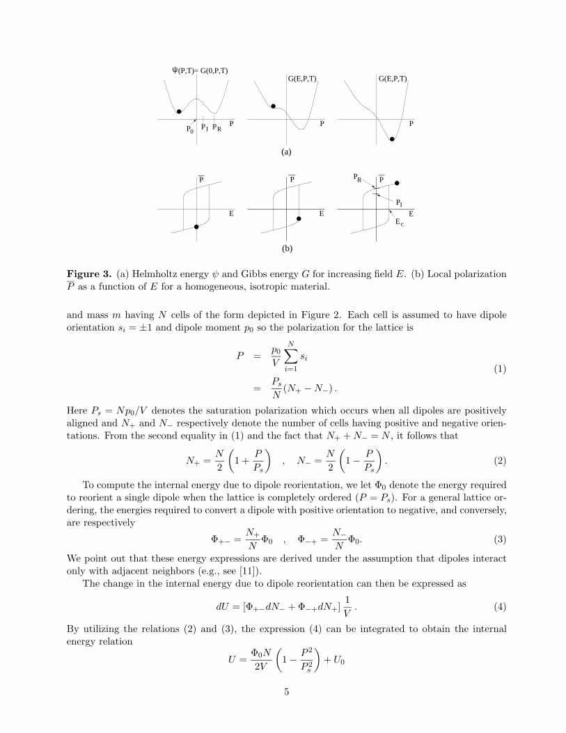
and a tetragonal form for T < Tc. We initially consider the idealized case of homogeneous materialshaving uniform lattices; hence for T > Tc, a unit cell at any point in the material will have the cubicionic structure illustrated for PbTi1−xO3 in Figure 2a. At temperatures below Tc, the materialsdistorts from the cubic to tetragonal form through the biasing of Ti4+ ions toward O2− pairs asillustrated for BaTiO3 on page 71 of [16]. In the absence of an applied electric field E, this ionicconfiguration produces a double well potential energy profile which varies as a function of the Ti4+

position. As depicted in Figure 3, the application of an electric field distorts the energy landscape anda dipole switch occurs when the equilibrium value determining the Ti4+ position exceeds the unstableequilibrium due to the central O2− pairs. At the macroscopic scale, this produces a discontinuousjump in the polarization as experimentally illustrated for single crystal BaTiO3 on pages 72-76 of [16].

2.1 Helmholtz Energy

We consider two techniques to quantify the Helmholtz free energy depicted in Figure 2c and 3b;the first is based on statistical mechanics principles and the second, while motivated by the first, isphenomenological.

Based on the assumption of material homogeneity, we consider a uniform lattice of volume V

3

Hel

mho

ltz F

ree

Ene

rgy

0(c)

Ti Displacement

xPb

(b)(a)

Ti O

Pb

O

TiP

Figure 2. (a) Perovskite structure of PbTiO3 in the cubic form above Tc. (b) Tetragonal structureof PbTiO3 for T < Tc and resulting spontaneous polarization. (c) Helmholtz free energy as a functionof Ti position along the x3-axis.

4

I

(b)

(a)

c

RI0

G(E,P,T)G(E,P,T)ψ(P,T)= G(0,P,T)

R

P P P P P P

E E

PP PP

EE

P

Figure 3. (a) Helmholtz energy ψ and Gibbs energy G for increasing field E. (b) Local polarizationP as a function of E for a homogeneous, isotropic material.

and mass m having N cells of the form depicted in Figure 2. Each cell is assumed to have dipoleorientation si = ±1 and dipole moment p0 so the polarization for the lattice is

P =p0

V

N∑i=1

si

=Ps

N(N+ −N−) .

(1)

Here Ps = Np0/V denotes the saturation polarization which occurs when all dipoles are positivelyaligned and N+ and N− respectively denote the number of cells having positive and negative orien-tations. From the second equality in (1) and the fact that N+ + N− = N , it follows that

N+ =N

2

(1 +

P

Ps

), N− =

N

2

(1− P

Ps

). (2)

To compute the internal energy due to dipole reorientation, we let Φ0 denote the energy requiredto reorient a single dipole when the lattice is completely ordered (P = Ps). For a general lattice or-dering, the energies required to convert a dipole with positive orientation to negative, and conversely,are respectively

Φ+− =N+

NΦ0 , Φ−+ =

N−N

Φ0. (3)

We point out that these energy expressions are derived under the assumption that dipoles interactonly with adjacent neighbors (e.g., see [11]).

The change in the internal energy due to dipole reorientation can then be expressed as

dU = [Φ+−dN− + Φ−+dN+]1V

. (4)

By utilizing the relations (2) and (3), the expression (4) can be integrated to obtain the internalenergy relation

U =Φ0N

2V

(1− P 2

P 2s

)+ U0

5

where U0 denotes the energy for the completely ordered state. Since internal energy measures arerelative, we take U0 = 0 in subsequent relations.

The Helmholtz energy for the lattice is given by

ψ = U − ST

where S denotes the entropy. From classical statistical mechanics arguments in combination withStirling’s formula (e.g., see [11]), the entropy is given by

S =k

Vln

[(NN+

)]

=k

Vln

[N !

N−! N+!

]

=kN

V

[ln 2− 1 + P/Ps

2ln

(1 +

P

Ps

)− 1− P/Ps

2ln

(1− P

Ps

)]

=−kN

2V Ps

[P ln

(P + Ps

Ps − P

)+ Ps ln

(1−

(P

Ps

)2)]

+ S0

where k denotes Boltzmann’s constant and S0 = kNV ln 2. As with U0, we neglect S0 in the final

relation for the Helmholtz energy since we are interested in a relative, rather than absolute, measureof energy.

The resulting Helmholtz free energy is

ψ(P, T ) =Φ0N

2V

[1− (P/Ps)2

]+

TkN

2V Ps

[P ln

(P + Ps

Ps − P

)+ Ps ln(1− (P/Ps)2)

]

=EhPs

2[1− (P/Ps)2

]+

EhT

2Tc

[P ln

(P + Ps

Ps − P

)+ Ps ln(1− (P/Ps)2)

].

(5)

In the second expression of (5), Eh = NΦ0V Ps

is a bias field and Tc = Φ0k denotes the Curie tempera-

ture for the material. As illustrated in Figure 4, the relation (5) yields a double well potential attemperatures T < Tc whereas behavior indicative of paraelectric materials is reflected by the singlepotential produced at T > Tc. However, the logarithmic nature of the entropic term reduces theefficiency of algorithms which employ this relation and makes it difficult to correlate parameters inthe model with physically measured properties of the data.

A second technique for constructing the free energy, which addresses these difficulties, is basedon the observation that for fixed temperatures, a first-order approximation to the Helmholtz relation(5) exhibits a quadratic dependence on the polarization in neighborhoods of all three equilibria. Thismotivates the piecewise quadratic definition

ψ(P ) =

12η(P + PR)2 , P ≤ −PI

12η(P − PR)2 , P ≥ PI

12η(PI − PR)

(P 2

PI− PR

), |P | < PI

(6)

for the Helmholtz energy for fixed temperature regimes. As illustrated in Figure 3a, PI and PR

respectively denote the positive inflection point and polarization at which the minimum occurs. Therelation between these points and local properties of the hysteresis kernel will be established insubsequent discussion. It will also be illustrated later that η can be interpreted as the reciprocalslope ∂E

∂P of the hysteron in the post-switching linear regime.

6

−0.25 −0.2 −0.15 −0.1 −0.05 0 0.05 0.1 0.15 0.21

1.01

1.02

1.03

1.04

1.05

1.06

1.07

1.08x 10

5

Polarization (C/m2)

Hel

mho

ltz F

ree

Ene

rgy

−0.25 −0.2 −0.15 −0.1 −0.05 0 0.05 0.1 0.15 0.21

1.05

1.1

1.15

1.2

1.25

1.3

1.35x 10

5

Polarization (C/m2)

Hel

mho

ltz F

ree

Ene

rgy

(a) (b)

Figure 4. Helmholtz free energy specified by (5) for (a) T < Tc, and (b) T > Tc.

2.2 Gibbs Energy

To construct a Gibbs free energy which exhibits the behavior depicted in Figure 3a, the relationUE = −p · E quantifying the potential energy of a dipole p in the field E is combined with theHelmholtz energy throughout the lattice to yield

G = ψ − EP (7)

for ψ given by (5) or (6). In the absence of applied stresses, the Gibbs relation (7) is used tocharacterize the energy landscape for homogeneous materials having a uniform lattice structure.

2.3 Local Average Polarization

The probability of obtaining the energy level G for a lattice volume V is specified throughBoltzmann principles to be

µ(G) = Ce−GV/kT (8)

where C is an integration constant chosen to yield a probability of 1 for integration over all admissibleinput values. For model identification, the volume V is typically chosen to yield relaxation behaviorappropriate for the material under consideration.

For a uniform input field E, the local average polarization at the lattice level is given by

P = x+ 〈P+〉+ x− 〈P−〉 (9)

where x+ and x− denote the fractions of dipoles having positive and negative orientations and 〈P+〉and 〈P−〉 are the expected polarization levels associated with positively and negatively orienteddipoles.

The evolution of the dipole fractions is specified by the differential equations

x+ = −p+−x+ + p−+x−

x− = −p−+x− + p+−x+

which can be simplified tox+ = −p+−x+ + p−+(1− x+) (10)

7

through the identity x++x− = 1. Here p+− denotes the likelihood of a dipole switching from positiveto negative orientation whereas p−+ denotes the likelihood of switching from negative to positive(we avoid defining p+− and p−+ as probabilities since they can be unbounded). The likelihoods arecomputed by specifying the probability of achieving the energy required for a jump multiplied bythe frequency at which jumps are attempted. This yields the relations

p+− =

√kT

2πmV 2/3

e−G(E,P0(T ),T )V/kT∫ ∞

P0(T )e−G(E,P,T )V/kT dP

p−+ =

√kT

2πmV 2/3

e−G(E,−P0(T ),T )V/kT∫ P0(T )

−∞e−G(E,P,T )V/kT dP

where P0(T ) is the unstable equilibrium of G and m denotes the mass of the lattice. The denominatorin both cases arises from evaluation of the integration constant C. When implementing the model,we typically replace P0(T ) by the inflections points PI and −PI , respectively, in the relations forp+− and p−+ to obtain

p+− =

√kT

2πmV 2/3

e−G(E,PI ,T )V/kT∫ ∞

PI

e−G(E,P,T )V/kT dP

p−+ =

√kT

2πmV 2/3

e−G(E,−PI ,T )V/kT∫ −PI

−∞e−G(E,P,T )V/kT dP

.

(11)

This simplifies the approximation of the integrals and can be motivated by observing that if oneconsiders the forces ∂G

∂P due to the applied field, maximum restoring forces occur at PI and −PI

(e.g., see pages 332-333 of [6]). Furthermore, for materials with low thermal activation, the pointsP0 and −PI coincide in the limit as thermal activation is reduced to zero for positive fields while PI

and P0 coincide for negative fields as illustrated in Figure 5.The expected polarizations are given by

〈P+〉 =∫ ∞

P0(T )Pµ(G) dP , 〈P−〉 =

∫ P0(T )

−∞Pµ(G) dP .

Specification of the probabilities using (8) and formulation of the integrals in terms of the inflectionpoints yields the relations

〈P+〉 =

∫ ∞

PI

Pe−G(E,P,T )V/kT dP∫ ∞

PI

e−G(E,P,T )V/kT dP

, 〈P−〉 =

∫ −PI

−∞Pe−G(E,P )V/kT dP∫ −PI

−∞e−G(E,P )V/kT dP

(12)

quantifying the expected polarizations respectively due to positively and negatively oriented dipoles.The summed products of the expectations and phase fractions (9) quantifies the local polarization

P at the lattice level. For materials which are homogeneous and isotropic, this local polarizationwill be uniform throughout the material and hence it will also quantify the macroscopic polarization

8

Ec

PI

P

Pmin P0Pmin

−PI

= − ηEP PR

PR

= ηEP PR+

E

P

− EP

(b)(a)

G ψ=

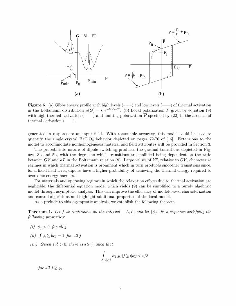
Figure 5. (a) Gibbs energy profile with high levels (– – –) and low levels (——) of thermal activationin the Boltzmann distribution µ(G) = Ce−GV/kT . (b) Local polarization P given by equation (9)with high thermal activation (– – –) and limiting polarization P specified by (22) in the absence ofthermal activation (——).

generated in response to an input field. With reasonable accuracy, this model could be used toquantify the single crystal BaTiO3 behavior depicted on pages 72-76 of [16]. Extensions to themodel to accommodate nonhomogeneous material and field attributes will be provided in Section 3.

The probabilistic nature of dipole switching produces the gradual transitions depicted in Fig-ures 3b and 5b, with the degree to which transitions are mollified being dependent on the ratiobetween GV and kT in the Boltzmann relation (8). Large values of kT , relative to GV , characterizeregimes in which thermal activation is prominent which in turn produces smoother transitions since,for a fixed field level, dipoles have a higher probability of achieving the thermal energy required toovercome energy barriers.

For materials and operating regimes in which the relaxation effects due to thermal activation arenegligible, the differential equation model which yields (9) can be simplified to a purely algebraicmodel through asymptotic analysis. This can improve the efficiency of model-based characterizationand control algorithms and highlight additional properties of the local model.

As a prelude to this asymptotic analysis, we establish the following theorem.

Theorem 1. Let f be continuous on the interval [−L, L] and let {φj} be a sequence satisfying thefollowing properties:

(i) φj > 0 for all j

(ii)∫

φj(y)dy = 1 for all j

(iii) Given ε, δ > 0, there exists j0 such that∫|y|≥δ

φj(y)|f(y)|dy < ε/3

for all j ≥ j0.

9

Then for x ∈ [−L, L], φk ∗ f converges to f ; that is∫φj(x− y)f(y)dy → f(x).

Proof. From (ii) it follows that

f(x) = f(x)∫

φj(y)dy =∫

f(x)φj(y)dy

so that for x ∈ [−L, L],

φj ∗ f(x)− f(x) =∫

φj(y)f(x− y)dy −∫

φj(y)f(x)dy

=∫

φj(y)[f(x− y)− f(x)]dy .

Furthermore, from the continuity of f , it follows that for fixed ε, there exists δ such that

|f(x− y)− f(x)| < ε/3

for |y| < δ. For this δ, we write

φj ∗ f(x)− f(x) =∫|y|<δ

φj(y)[f(x− y)− f(x)]dy +∫|y|≥δ

φj(y)[f(x− y)− f(x)]dy < ε

for sufficiently large j. The integral over the region |y| < δ is bounded by ε/3 due to the continuityof f whereas the integral over |y| ≥ δ is bounded by 2ε/3 for sufficiently large j as a result of (iii).The convergence follows directly. ¤

We note that if we replace property (iii) by the requirement∫|y|≥δ

φj(y)dy < ε

and add the assumption that f is measurable and bounded on lR, the sequence φj is termed a Diracsequence on lR, and Theorem 1 is a 1-D version of Theorem 3.1 from page 228 of [13].

2.4 Asymptotic Polarization Relation in Absence of Thermal Activation

We now consider initial dipole fractions x−, x+, and a positive field E for which G(Pmin) ≤ G(P0)and G(Pmin) < G(Pmin) as depicted in Figure 5a. For simplicity, we consider the piecewise quadraticHelmholtz free energy model (6) and note that analogous asymptotic analysis holds for the statisticalmechanics model (5). In this case, the minima

Pmin(E) =E

η− PR , Pmin(E) =

E

η+ PR (13)

result from the necessary condition ∂G∂P = 0. The coercive field for which Pmin = P0 = −PI is given

byEc = η(PR − PI) . (14)

10

We illustrate first that for kT/V > 0, the Boltzmann probability (8) exhibits Gaussian behaviorin neighborhoods of Pmin and Pmin with variance proportional to kT/V . We will also illustrate thatin the limit kT/V → 0, µ(G) converges to a Dirac distribution.

For P < −PI , µ(G) can be formulated as

µ(G) =e−[ 1

2η(P+PR)2−EP ]V/kT∫ −PI

−∞e−[ 1

2η(P+PR)2−EP ]V/kT dP

=e−(P−P min)2ηV/2kT∫ −PI

−∞e−(P−P min)2ηV/2kT dP

= C(T, β)e−(P−P min)2/2β2

(15)

where

β =

√kT

ηV

C(T, β) =[∫ −PI

−∞e−(P−P min)2/2β2(T )dP

]−1

.

(16)

We now let j = 1/β and define the sequence

φj(P ) =

{C(T, j)e−(P−P min)2j2/2 , P ≤ −PI

0 , P > −PI .

Since {φj} satisfies (i)-(iii) of Theorem 1, and hence constitutes a Dirac sequence, it follows that

limkT/V→0

µ(G) = limj→∞

φj(P )

= δ(P − Pmin).(17)

Analogous behavior is exhibited at Pmin.The Gaussian behavior of µ, quantified by (15), is depicted in Figure 5a. From the definition of

β, it follows that a decrease in thermal activation is reflected as a decrease in the variance. Thisimplies that a smaller number of dipoles achieve the energy required to overcome the energy barrierwhich yields steeper transitions in the relation between E and P as depicted in Figure 5b.

We now illustrate that the solution to the model (9) converges to the piecewise linear kernelspecified by (13). It is first noted that as kT/V → 0, the limiting solution to (10) is

x+ = x+ + (1− x+)h(P + PI)

=

{x+ , E < Ec

1 , E > Ec

(18)

where the local coercive field Ec is given by (14) and h denotes the Heaviside function. Correspondingvalues for x− are determined through the relation x+ + x− = 1.

11

The expected polarization due to positively oriented dipoles is

〈P+〉 = limkT/V→0

∫ ∞

PI

Pe−G(E,P )V/kT dP∫ ∞

PI

e−G(E,P )V/kT dP

= limj→∞

j√2π

∫ ∞

PI

Pe−(P−Pmin)2j2/2 dP

j√2π

∫ ∞

PI

e−(P−Pmin)2j2/2 dP

= Pmin

(19)

with the limits in the numerator and denominator evaluated using Theorem 1 with f(P ) = P andf(P ) = 1 for P > P0, f(P ) = 0 for P < P0, respectively. Similarly, the limiting value of 〈P−〉 is

〈P−〉 = Pmin . (20)

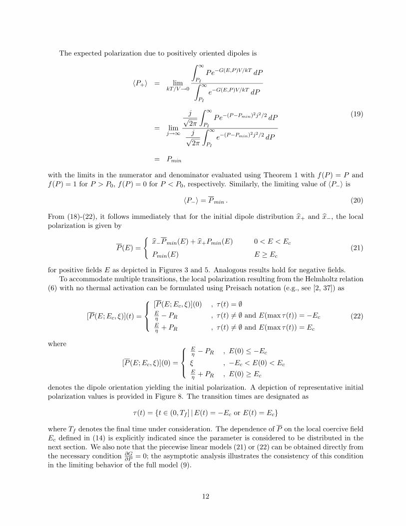
From (18)-(22), it follows immediately that for the initial dipole distribution x+ and x−, the localpolarization is given by

P (E) =

{x−Pmin(E) + x+Pmin(E) 0 < E < Ec

Pmin(E) E ≥ Ec

(21)

for positive fields E as depicted in Figures 3 and 5. Analogous results hold for negative fields.To accommodate multiple transitions, the local polarization resulting from the Helmholtz relation

(6) with no thermal activation can be formulated using Preisach notation (e.g., see [2, 37]) as

[P (E; Ec, ξ)](t) =

[P (E; Ec, ξ)](0) , τ(t) = ∅Eη − PR , τ(t) 6= ∅ and E(max τ(t)) = −Ec

Eη + PR , τ(t) 6= ∅ and E(max τ(t)) = Ec

(22)

where

[P (E; Ec, ξ)](0) =

Eη − PR , E(0) ≤ −Ec

ξ , −Ec < E(0) < Ec

Eη + PR , E(0) ≥ Ec

denotes the dipole orientation yielding the initial polarization. A depiction of representative initialpolarization values is provided in Figure 8. The transition times are designated as

τ(t) = {t ∈ (0, Tf ] |E(t) = −Ec or E(t) = Ec}

where Tf denotes the final time under consideration. The dependence of P on the local coercive fieldEc defined in (14) is explicitly indicated since the parameter is considered to be distributed in thenext section. We also note that the piecewise linear models (21) or (22) can be obtained directly fromthe necessary condition ∂G

∂P = 0; the asymptotic analysis illustrates the consistency of this conditionin the limiting behavior of the full model (9).

12

E

(a)

E

R

(b)

PP P

PI

Ec

Figure 6. (a) Kernel provided by (22), and (b) kernel provided by (23).

Similar analysis can be used to specify the hysteresis kernel which results when G is constructedusing the Helmholtz relation (5) derived through statistical mechanics arguments. The determinationof P through solution of ∂G

∂P = 0 in this case yields

P (E; Eh) = Pstanh(

E + EhP/Ps

EhT/Tc

)

= Pstanh(

E + αP

a(T )

) (23)

whereα =

Eh

Ps, a(T ) =

EhT

Tc. (24)

The behavior of P specified by (23) is compared in Figure 6 with that defined by (21) or (22) whichwas derived from the piecewise quadratic Helmholtz energy. While the two representations yieldsimilar kernel behavior as dipole switching occurs, the model (23) predicts a local saturation valueof Ps and decreasing slope for increasing field whereas the model (22) predicts linear behavior afterdipole switching with slope 1

η .The Ising model (23) has been employed in a number of hysteresis models for ferroelectric mate-

rials and its ubiquity is due to the common underlying assumption that dipoles are aligned in onlytwo configurations: in the direction of the applied field or diametrically opposite to it. As detailed in[32], quantification of the electrostatic energy under this assumption yields the Ising model whereasthe relaxed assumption that dipoles can orient uniformly yields a Langevin model, which agrees withthe Ising model through first-order terms but predicts a slower saturation rate. In both cases, thesemodels were employed to quantify the anhysteretic kernel as an initial step in the development of amacroscopic hysteresis model [32, 33]. The theory developed here differs from the domain wall theoryin [32, 33] in the sense that the Ising model directly quantifies the energy landscape at the latticelevel whereas it provides only an intermediate step in the domain wall theory. The saturation be-havior of the Ising relation has also motivated its use in phenomenological models. Translates of theform P = Pstanh(E ±Ec) were employed by Zhang and Rogers [39], and r(x) = tanh(x) provides asuitable choice for the ridge functions employed in generalized Preisach, or Krasnolselskii-Pokrovskii,characterizations [2, 3]. The model presented here differs in that it focuses on an energy formulationfor domain processes. This yields a low-order model which, as illustrated in the examples, ensuresclosure of biased minor loops.

13

3 Polycrystalline Materials with Variable Effective Fields

The local polarization relations (9), (22) and (23) were derived under the assumption of homogeneousand isotropic material properties and uniform effective fields Ee = E throughout the materials. Theconsideration of the local relations throughout the material yields global models which predict instan-taneous transitions at the coercive field as illustrated in Figures 4, 5 and 6. While such global modelscan accurately quantify single crystal behavior of the type experimentally measured for BaTiO3 (e.g.,see page 76 of [16]), they do not accurately predict the more gradual transition through the remanentpolarization measured in polycrystalline ferroelectric materials. In this section, we incorporate theeffects of nonuniform lattice configurations, polycrystallinity, and variable effective fields to providea macroscopic model which accurately characterizes hysteresis in a variety of ferroelectric materialsand ensures closure of biased minor loops.

3.1 Distributions in Remanence Polarization, Lattice, and Coercive Field

As illustrated in Figure 7, nonuniformities in the lattice produce a distribution of Helmholtz andGibbs free energy profiles which can be manifested as variations in the local coercive field and localremanent polarization and can produce differing saturation behavior after dipole switching. Addi-tional variations in the free energy relations will be produced by stress nonhomogeneities, nonuniformlattice orientations across grain boundaries, and crystalline anisotropies.

(i) (ii)

Pb

Ti

O

(i) (ii)

G

P P

G

(i) (ii)

(c)

(b)

P

E

P

E

(a)

PRP

I

Figure 7. (a) Nonuniform lattice and polycrystalline structure for PZT; (b) Free energies associatedwith lattice widths (i) and (ii); (c) Variations in hysteresis kernel due to differing free energies.

14

For the piecewise quadratic Helmholtz model (6), the variability in the lattice structure canbe incorporated by considering PR, PI or Ec = η(PR − PI) to be manifestations of an underlyingdistribution rather than fixed values as assumed in the previous section for single crystals havinguniform lattices. For this model, we consider variations in the local coercive field Ec and make theassumption that it can be modeled by a log-normal distribution to incorporate the requirement thatEc > 0. This yields the relation

[P (E)](t) =∫ ∞

0[P (E; Ec, ξ)](t)f(Ec) dEc

for the macroscopic polarization where the density f is specified by

f(Ec) = c1 exp

{−

[ln(Ec/Ec)

2c

]2}

(25)

and P is given by (9) or (22). Here c, c1 and Ec are positive constants. In [8], it is illustrated thatif c is small compared with Ec, the mean and variance have the approximate values

〈Ec〉 ≈ Ec , σ ≈ 2Ec c . (26)

As will be illustrated in the examples of Section 4, the relation (26) can be used to obtain initialparameter estimates based on attributes of measured experimental data. For materials in which thetransition during hysteresis is relatively gradual, a second choice for f is a normal distribution withmean Ec and variance σ. The lower integration limit of 0 should be retained to enforce nonnegativelocal coercive fields.

3.2 Nonuniform Effective Fields

The second extension employed to obtain a macroscopic model for the polarization entails theconsideration of effective fields in the material. As noted in [1, 15, 32, 33], the applied field inferroelectric materials is augmented by fields generated by neighboring dipoles which produce non-homogeneous effective fields in the materials. This produces variations about the applied field whichcan significantly alter the measured polarization. To incorporate these field variations, we considerthe effective field to be normally distributed about the applied field. For fixed Ec, the polarizationin this case is given by

[P (E)](t) =∫ ∞

−∞c2[P (Ee; Ec, ξ)](t)e−(E−Ee)2/bdEe . (27)

The introduction of variations in the effective field produces domain switching in advance of theremanence point in accordance with observations from experimental data.

The complete macroscopic polarization model for nonhomogeneous, polycrystalline materials withvariable effective fields, as based on the piecewise quadratic Helmholtz model (6), is then given by

[P (E)](t) = C

∫ ∞

0

∫ ∞

−∞[P (Ee + E, Ec, ξ)](t)e−E2

e/be−[ln(Ec/Ec)/2c]2dEedEc (28)

where P is specified by (9) or (22). We note that while the model (28) incorporates certain relax-ation mechanisms, it does not incorporate dynamic elastic effects. Hence this formulation of thepolarization model should be restricted to low frequency drive regimes.

15

Similar arguments can be employed to construct a macroscopic polarization model based on theHelmholtz free energy relation (5) obtained through statistical mechanics analysis. In this case, weassume that the bias field Eh is a manifestation of an underlying log-normal distribution to obtainthe global relation

[P (E)](t) = C

∫ ∞

0

∫ ∞

−∞[P (Ee + E, Eh, ξ)](t)e−E2

e/be−[ln(Eh/Eh)/2c]2dEedEh. (29)

Here P is specified by (9) or (23).The polarization behavior predicted by (29) differs from that of (28) primarily at high input

field levels. The E-P behavior predicted by (28) reflects the linear behavior associated with thehysteresis kernel (22) after completion of dipole switching whereas the E-P curve produced by (29)saturates to zero slope due to the behavior of the hyperbolic tangent kernels. While both models areappropriate for a number of materials, the saturation behavior and ease with which the respectivemodels can be implemented are effective criteria for choosing between the models (28) and (29) fora given application.

3.3 Implementation Issues

To implement the models (28) or (29), it is necessary to approximate the integrals. This canbe accomplished on the semi-infinite domain using Gauss-Laguerre quadrature and on the infinitedomain using Gauss-Hermite quadrature (e.g., see pages 698-699 of [40]). Alternatively, the expo-nential decay of the kernels can be employed to truncate the domains to finite intervals appropriatefor Gauss-Legendre formulae (see Figure 8a). In all cases, approximation of (28) yields expressionsof the form

[P (E)](t) = C

Ni∑i=1

Nj∑j=1

[P (Eej + E; Eci , ξi)](t)e−E2

ej/b

e−[ln(Eci/Ec)/2c]2viwj (30)

with a similar relation resulting from the approximation of (29). Here Eej , Eci denote the abscissasassociated with respective quadrature formulae and vi, wj are the respective weights.

For the examples reported in Section 4, we employed composite Gauss-Legendre quadrature ontruncated intervals chosen to be commensurate with nontrivial values of the integrands. To illustrate,we provide the abscissas and weights employed in the approximation of the integral (27) on thetruncated domain [−L, L] using a four point composite quadrature rule. Letting hj = −L + jh, thequadrature points and weights on each subinterval [hj−1, hj ] are

Eej1 = hj−1 + h

[12 −

√15+2

√30

2√

35

], wj1 = 49h

12(18+√

30)

Eej2 = hj−1 + h

[12 −

√15−2

√30

2√

35

], wj2 = 49h

12(18−√30)

Eej3 = hj−1 + h

[12 +

√15−2

√30

2√

35

], wj3 = 49h

12(18−√30)

Eej4 = hj−1 + h

[12 +

√15+2

√30

2√

35

], wj4 = 49h

12(18+√

30).

The quadrature points and initial polarization values ξj for E = 0, P = 0, with the hysteresis kernel(22), are depicted for Nq = 2 (Nj = 8) in Figure 8b.

16

EcEc Ec

x

xxx

xx x

x

(d)

(a)

(b)

(c) Ec

E=0

P

−L L −L L

Figure 8. (a) Decay exhibited by f2(Ee) = e−E2e/b and truncated domain [−L, L]. (b) Gaussian

quadrature points • and initial local polarization values ξj (indicated by x) for Nj = 8. (c) Log-normal density f(Ec) = c1e

−[ln(Ec/Ec)/2c]2 having mean Ec. (d) Distribution of hysteresis kernelshaving coercive fields Ec.

A second implementation issue concerns the manner through which the conditional definitionsin (22) are evaluated if this kernel is employed in the hysteresis model. While it is algorithmicallystraightforward to implement these conditions using the transition times τ(t), this must be donefor all quadrature points Eej and Eci for each input field value. Implementation in this mannersignificantly diminishes the speed of the model evaluation and would likely prohibit the use of themodel for real-time control design and implementation.

An alternative is to formulate the local polarization (22) as

P =E

η+ PR∆ (31)

where ∆ = 1 if evaluating on the upper branch of the kernel and ∆ = −1 if evaluating on the lowerbranch. The crux of the algorithm focuses on the efficient construction of ∆ which accommodatesthe vector nature of the effective field values and coercive fields resulting from the quadrature ofthe integrals. Intuitively, the local polarization values associated with each effective field value Eej

will jump when they reach a coercive field Eci . Because both the effective and coercive field valuesare distributed, as depicted in Figure 8, this leads to Ni × Nj relations which must be checked foreach input field value E. Hence for the distributed algorithm, ∆ is an Ni × Nj matrix in whichthe ijth element specifies whether the jth effective field value Eej has crossed the ith coercive valueEci to determine whether the associated polarization value is on the upper or lower branch of thehysteron. The high efficiency of the algorithm is achieved by employing algebraic matrix operationsto construct ∆ rather than conditional statements implemented through if-then constructs.

17

To illustrate the algorithm used to compute P using the approximate relation (30), with P givenby (22), we first define the following matrices

∆init =

−1 · · · −1 1 · · · 1...

......

...−1 · · · −1 1 · · · 1

Ni×Nj

, Ec =

Ec1 · · · Ec1...

...EcNi

· · · EcNi

Ni×Nj

Ek =

Ek + Ee1 · · · Ek + EeNj

......

Ek + Ee1 · · · Ek + EeNj

Ni×Nj

, O =

1 · · · 1...

...1 · · · 1

Ni×Nj

and weight vectors

W T =[w1e

−E2e1

/b, · · · , wNje−E2

eNj/b

]1×Nj

V T =[v1e

−[ln(Ec1/Ec)/2c]2 , · · · , vNie−[ln(EcNi

/Ec)/2c]2]1×Ni

where Ek = E(tk) is the kth value of the input field. The polarization Pk ≈ P (Ek) is then specifiedby the following algorithm.

Algorithm 1.

∆ = ∆init

P = 1ηEc + PRO

for k = 1 : Nk

P = 1ηEk + PR∆

dE = Ek − Ek−1

∆ = sgn((Ek − sgn(dE)Ec). ∗ (P − sgn(dE)P ). ∗ P )

P = 1ηEk + PR∆

Pk = CV T PW

end

In this algorithm, .∗ indicates componentwise matrix multiplication and sgn denotes the signumfunction. Depending on the methods used for programming, the use of Algorithm 1 rather thanutilizing conditional if-then constructs can reduce runtimes by factors in excess of 100 so that fullmultiloop model simulations run in the order of seconds on a workstation. This level of efficiency isnecessary to achieve real-time implementation of control algorithms utilizing this model.

4 Model Validation

To illustrate attributes of the model, we consider two sets of examples. In the first, the capabilityof the model to characterize symmetric, major loop properties of PZT5A, PZT5H and PZT4 isillustrated through comparison with experimental data. For each compound, model parameters

18

are estimated through a least squares fit to data at high drive levels and the resulting model isused to predict the model behavior in lower drive regimes. In all cases, quasistatic drive regimesare considered. The second example illustrates numerically the capability of the model to quantifybiased minor loop behavior including Raleigh loops at low drive levels and multiply nested loops atintermediate levels. In concert, these examples illustrate the flexibility of the model for a variety ofmaterials and operating conditions.

4.1 Determination of Parameters

The continuous model (28) or discretized model (30) contains the parameters PR, η, b, Ec, c andC which must be specified when quantifying a specific PZT compound. Similar parameters arise inthe model derived through statistical mechanics principles. Asymptotic analysis can be employed toobtain initial parameter choice which can then be employed in various least squares formulations todetermine parameters which optimize model fits and predictions.

As illustrated in Figure 5, PR denotes the local remanence polarization for a domain and η is thereciprocal of the slope in the E-P relation after switching. The inclusion of polycrystallinity, variableeffective fields and material nonhomogeneities through the density analysis in Section 3 makes itdifficult to correlate the remanence polarization measured for the bulk material with the local valuePR; hence PR is typically estimated solely through a least squares fit to the data. Moreover, forthe linear relations (22) or (31) for the kernel P , PR and C produce analogous scaling in the bulkpolarization so that they can be combined when estimating parameters. The slope of the localkernel relations scales through the stochastic homogenization process so bulk measurements of thereciprocal slope dE

dP provide initial estimates for η. The distribution f , defined in (25), quantifies

Ei

Ei

E

P

}

E

Pη∼∼ dP

dE

ModelData

Ec

b

(a) (b)

Emin Emax(c)

Figure 9. (a) Asymptotic relations between the parameters η,Ec, b and the slope of the P -E rela-tion after switching, the coercive field and the point where switching commences before remanence.(b) The absolute metric (32) and Euclidean metric (34) between data and the model prediction.(c) Cosine filter (33) used to minimize least squares differences in the switching region.

19

the coercive properties of the E-P relation. The mean Ec quantifies the point at which the primaryswitching occurs as illustrated in Figure 9a; hence Ec is asymptotically given by the coercive fieldfor the bulk material. The variance σ ≈ 2Ecc quantifies the variability in local coercive fields so thatmaterials with steep coercive transitions yield small values of c whereas large parameter values arerequired when characterizing materials with gradual bulk switching. The parameter b quantifies thevariance in the effective field which determines, in part, the degree to which switching occurs beforeremanence is reached. Materials with nearly linear E-P relations at remanence yield small values ofb whereas large values are required to accommodate significant switching before remanence.

Hence physical properties of the data yield initial estimates for η and Ec and provide quali-tative techniques for ascertaining b, c, PR and C. This significantly facilitates the implementationof least squares techniques used to determine model parameters and update these parameters toaccommodate slowly changing operating conditions.

Three least squares techniques have been considered to accommodate the switching and saturationbehavior inherent to hysteresis data. To formulate the least squares problems, let (Ei, Pi), i =1, · · · ,N , denote the field and corresponding polarization data measured throughout the hysteresiscycle. Furthermore, let P (Ei; q) denote parameter-dependent model solutions provided by (28), (29)or (30). For admissible parameters q ∈ Q, we then consider the following optimization problems:

minq

N∑i=1

∣∣∣P (Ei; q)− Pi

∣∣∣2 , (32)

minq

N∑i=1

µi

∣∣∣P (Ei; q)− Pi

∣∣∣2 , µi ≡ cos

[2π · Ei − Emin

Emax − Emin

]+ α, (33)

minq

N∑i=1

d(P (Ei; q)− Pi

). (34)

The functional (32) penalizes absolute differences between the data and model. As illustrated inFigure 9b, it will produce model fits which tend to be more accurate in the high gradient switchingregime than in the low gradient saturation region. For applications which require high accuracythroughout the drive range, two techniques can be employed to modify the manner through whichthe difference between the model and data are penalized. One alternative is to employ the functional(33) which weights the data in the saturation region more heavily through a cosine filter of the typeillustrated in Figure 9c. A more accurate, but computationally more intensive, technique employsthe Euclidean metric d which minizes the distance between the model and data as illustrated inFigure 9b. For each functional, initial parameter choices q0 are obtained through the previouslydiscussed asymptotic relations or a priori material information.

4.2 Experimental Validation for PZT5A, PZT5H and PZT4

To illustrate the accuracy and flexibility of the model and parameter estimation techniques fora variety of compounds, we consider the characterization of PZT5A, PZT5H and PZT4 wafers.In all cases, data was collected at 200 mHz to minimize frequency effects. For consistency, thediscretized model (30), with P given by (22) or (31), was employed in all three cases. However,we note that analogous results have been obtained with the kernel (9) and the discretized versionof the statistical mechanics model (29). Finally, the limits Ni = Nj = 80 in (30) – obtained usingNq = Np = 20 subdivisions with the 4 point Gaussian rule – ensured convergence of the Gaussianquadrature routines.

20

PZT5A

We consider first the characterization of hysteresis exhibited by PZT5A for various input fieldlevels. Data was collected from a rectangular 1.7 cm × 0.635 cm × 0.0381 cm wafer at peak voltagesranging from 600 V to 1600 V. Corresponding field values were computed using the relation

E = V/h

where h = 3.81× 10−4 m denotes the thickness of the wafer. The resulting hysteretic E-P relationsare plotted in Figure 10.

The polarization was modeled using the relation (30) with the piecewise linear kernel (22). Thecoercive field for the 1600 V data is 1.2 × 106 V/m and the slope after field reversal in saturationis 3.6 × 108. These two values were respectively employed as initial estimates for Ec and η. Thefunctional (32) was then employed to estimate the parameters PR = 0.04 C/m2, Ec = 0.96507 ×106 V/m, η = 9×108, c = 0.3582 V2/m2, b = 2.1407×1011 V2/m2 and C = 8.57×10−12 through a fitto the 1600 V data. The model with these parameter values was then used to predict the hystereticE-P relation at the 600 V, 800 V and 1000 V input levels yielding the fits plotted in Figure 10. It isobserved that the model accurately quantifies the hysteresis through the switching region at 1600 Vbut is less accurate near saturation since errors in this region are penalized less by the absolutefunctional (32). The accuracy of the predictions at the lower drive levels attests to the flexibility ofthe model for quantifying the E-P relation through a wide range of field inputs.

The use of the cosine-weighted functional (33) yields the parameters PR = 0.04 C/m2, Ec =0.866010×106 V/m, η = 9.5×108, c = 0.4272 V2/m2, b = 1.9754×1011 V2/m2 and C = 7.9926×10−12

and produces a model fit with slightly improved accuracy in the saturation region but less accuracynear the coercive field and at low drive levels (see Figure 11). Both algorithms provide sufficientaccuracy for quantifying hysteresis inherent to PZT5A for a broad range of applications.

−5 0 5−0.5

0

0.5600 V

−5 0 5−0.5

0

0.5800 V

−5 0 5−0.5

0

0.51000 V

−5 0 5−0.5

0

0.51600 V

Figure 10. PZT5A data (– – –) and model predictions (——) with the parameters PR = 0.04 C/m2,Ec = 0.96507×106 V/m, η = 9×108, c = 0.3582 V2/m2, b = 2.1407×1011 V2/m2, C = 8.57×10−12

determined by the absolute least squares functional (32). Abscissas: electric field (MV/m), ordinates:polarization (C/m2).

21

−5 0 5−0.5

0

0.5600 V

−5 0 5−0.5

0

0.5800 V

−5 0 5−0.5

0

0.51000 V

−5 0 5−0.5

0

0.51600 V

Figure 11. PZT5A data (– – –) and model predictions (——) with the parameters PR = 0.04 C/m2,Ec = 0.866010 × 106 V/m, η = 9.5 × 108, c = 0.4272 V2/m2, b = 1.9754 × 1011 V2/m2, C =7.9926 × 10−12 determined by the cosine-weighted least squares functional (33). Abscissas: electricfield (MV/m), ordinates: polarization (C/m2).

PZT5H

To illustrate the performance of the model for characterizing a second soft PZT compound, weconsider data collected from a 3.81 cm × 0.635 cm × 0.0381 cm PZT5H wafer at input levels rangingfrom 600 V to 2200 V. As with the PZT5A sample, data was collected at 200 mHz to minimizefrequency effects.

For this data set, parameters were estimated through a fit to the 2200 V data and the resultingmodel was used to predict the hysteretic E-P relation at lower drive levels. Initial values for Ec andη were obtained from the coercive field Ec = 0.9×106 V/m and reciprocal slope dE

dP = 3.7×108, aftersaturation, for the 2200 V data. The absolute least squares functional (32) yielded the parametersPR = 0.04 C/m2, Ec = 0.747690 × 106 V/m, η = 6.5 × 108, c = 0.2612 V2/m2, b = 2.8425 ×1011 V2/m2, C = 1.1526× 10−11 and fits depicted in Figure 12. The Euclidean metric (34) yieldedthe parameter values PR = 0.04 C/m2, Ec = 0.698990 × 106 V/m, η = 6.5 × 108, c = 0.3439V2/m2, b = 3.2407× 1011 V2/m2, C = 8.0932× 10−12 and fits depicted in Figure 13. It is observedthat because the absolute metric heavily penalizes discrepancies in high gradient regions, the fits inFigure 12 are very accurate in the coercive region but saturate too quickly. The use of the Euclideanmetric provides more uniform penalties throughout the drive range and hence provides a model whichis accurate both in switching and saturation.

PZT4

The final compound that we consider is the hard material PZT4. Data collected from a 3.81 cm× 0.635 cm × 0.381 cm wafer at input levels of 600 V through 1800 V is plotted in Figure 14. Forthe 1800 V input, the coercive field 1.42 × 106 V/m reflects that more energy is required to turndipoles than in the softer PZT5 compounds.

22

−5 0 5−0.5

0

0.5600 V

−5 0 5−0.5

0

0.51000 V

−5 0 5−0.5

0

0.51600 V

−5 0 5−0.5

0

0.52200 V

Figure 12. PZT5H data (– – –) and model predictions (——) with the absolute least squaresfunctional (32) used to determine the parameters PR = 0.04 C/m2, Ec = 0.747690 × 106 V/m,η = 6.5× 108, c = 0.2612 V2/m2, b = 2.8425× 1011 V2/m2, C = 1.1526× 10−12. Abscissas: electricfield (MV/m), ordinates: polarization (C/m2).

−5 0 5−0.5

0

0.5600 V

−5 0 5−0.5

0

0.51000 V

−5 0 5−0.5

0

0.51600 V

−5 0 5−0.5

0

0.52200 V

Figure 13. PZT5H data (– – –) and model predictions (——) with the Euclidean least squaresfunctional (34) used to determine the parameters PR = 0.04 C/m2, Ec = 0.698990 × 106 V/m,η = 6.5× 108, c = 0.3439 V2/m2, b = 3.2407× 1011 V2/m2, C = 8.0932× 10−12. Abscissas: electricfield (MV/m), ordinates: polarization (C/m2).

23

−4 −2 0 2 4−0.5

0

0.5600 V

−4 −2 0 2 4−0.5

0

0.51000 V

−4 −2 0 2 4−0.5

0

0.51200 V

−4 −2 0 2 4−0.5

0

0.51800 V

Figure 14. PZT4 data (– – –) and model predictions (——) with the parameters PR = 0.045 C/m2,Ec = 1.05×105 V/m, η = 4.0×108, c = 0.3018 V2/m2, b = 2.1924×1011 V2/m2, C = 6.8287×10−12.Abscissas: electric field (MV/m), ordinates: polarization (C/m2).

The three functionals (32)-(34) yield roughly equivalent parameters and the model response withthe parameters PR = 0.045 C/m2, Ec = 1.05 × 105 V/m, η = 4.0 × 108, c = 0.3018 V2/m2,b = 2.1924 × 1011 V2/m2, C = 6.8287 × 10−12, estimated through a fit to the 1800 V data, iscompared with the data in Figure 14. It is observed that while model is very accurate in the highdrive regime, it does not fully quantify the sharp transition prior to coercivity due to limitationsresulting from the choice of the lognormal and normal functions used to respectively characterizethe densities of the coercive and effective fields. This tendency is accentuated when the model issubsequently used to predict the 600 V E-P relation. While the model provides sufficient accuracyfor applications such as control design, the discrepancy illustrates that improvements can be madein the model when modeling hard compounds. We are presently investigating the development ofhigher-order kernels and techniques for identifying general densities to provide additional accuracyfor high performance applications which utilize PZT4 transducers.

4.3 Biased Asymmetric Minor loops

To illustrate the capability of the model to quantify biased minor loops, the field plotted inFigure 15a was input to the model to generate the E-P relation depicted in Figure 15b. Theparameters were taken to be PR = 0.04 C/m2, Ec = 0.698990 × 106 V/m, η = 6.5 × 108, c =0.6877 V2/m2, b = 3.2407 × 1011 V2/m2, C = 8.0932 × 10−12 which are close to those identifiedfor PZT5H (the parameters were modified slightly to highlight aspects of the biased loops). Loop 1illustrates the capability of the model to characterize the quadratic Raleigh behavior experimentallyobserved for low drive levels whereas Loop 2 illustrates that the model enforces closure of biased,asymmetric minor loops on the initial polarization curve. The continuity in slope of the initialcurve, following the closure of Loop 2, illustrates that the model incorporates the deletion property

24

5 10 15 20 25 30 35 40 45 50−2

−1.5

−1

−0.5

0

0.5

1

1.5

2

Time (sec)

Fie

ld (

MV

/m)

−2 −1.5 −1 −0.5 0 0.5 1 1.5 2−0.5

−0.4

−0.3

−0.2

−0.1

0

0.1

0.2

0.3

0.4

0.5

Electric Field (MV/m)

Pol

ariz

atio

n (C

/m2 )

1

2

34

5

6

(a) (b)

Figure 15. (a) Field input E, and (b) polarization predicted by the discretized model (30).

which, along with congruency, forms one of the necessary and sufficient conditions for classicalPreisach models [8]. Loops 3 and 4 illustrate the ability of the model to enforce closure of multiplynested loops while Loop 5 encapsulates biased behavior near saturation. When combined with theexperimental results in Section 4.2, the behavior depicted here provides the model with substantialflexibility for material characterization and control design.

5 Concluding Remarks

The theory presented in this paper provides a technique for quantifying constitutive nonlinearitiesand hysteresis inherent to piezoelectric compounds in a manner conducive to bulk material char-acterization and model-based control design. Through the combination of free energy analysis atthe lattice or domain level with the assumption that certain physical parameters are stochasticallydistributed, macroscopic models having a small number of parameters (5-6) are constructed. Fur-thermore, several of these parameters can be correlated with physical attributes of the E-P datato facilitate parameter identification and model updating to accommodate changing operating con-ditions. The model accommodates transient dynamics in the E-P relation, enforces return pointmemory, and guarantees the closure of both symmetric and biased, asymmetric minor loops. Themodel does not enforce congruency in the saturation regions of the E-P curve which reflects themeasured behavior of the materials in these regions.

The numerical examples and comparison with experimental data illustrate low-frequency, fixed-temperature capabilities of the model. In its present formulation, however, it also incorporates certainrelaxation mechanisms and temperature-dependencies. The latter effect has been validated in thecontext of relaxor ferroelectric compounds (PMN) and a comprehensive set of examples illustratingthe quantification of these properties in PZT will appear in a future publication. The model in itspresent form does not incorporate polarization changes due to variable stresses and these extensionsare under current investigation.

The use of Algorithm 1 renders the model highly efficient so that multiloop simulations run inthe order of seconds on an aging and overworked workstation. In the algorithm described in [34], themonotonicity of the modeled E-P relation was invoked to construct an inverse model for inclusion infeedforward or feedback loops to linearize (at least approximately) the response of actuators operating

25

in nonlinear and hysteretic and nonlinear regimes. The analogous magnetic model and inverse areemployed in [17] to construct robust control designs to achieve high accuracy, high speed positioncontrol for Terfenol-D transducers. Hence the unified nature of the modeling approach facilitatesunified control designs that utilize model-based inverse compensators.

Acknowledgements

The research of R.C.S. was supported in part through the NSF grant CMS-0099764 and in part bythe Air Force Office of Scientific Research under the grant AFOSR-F49620-01-1-0107. The researchof S.S. was supported in part by the National Science Foundation through the grant DMI-0134464.The research of J.S. was supported through the NSF grant CMS-0099764 and the NSF subcontract420-20-78 through Iowa State University. The authors thank Marcelo Dapino, Julie Raye, and ananonymous referee for providing input which helped to improve the paper.

Note: Center for Research in Scientific Computation Technical Reports can be accessed at the website http://www.ncsu.edu/crsc/reports.html.

References

[1] J.C. Anderson, Dielectrics, Reinhold Publishing Corporation, New York, 1964.

[2] H.T. Banks, A.J. Kurdila and G. Webb, “Identification of hysteretic control influence operatorsrepresenting smart actuators Part I: Formulation,” Mathematical Problems in Engineering, 3,pp. 287-328, 1997.

[3] H.T. Banks, A.J. Kurdila and G. Webb, “Identification of hysteretic control influence opera-tors representing smart actuators Part II: Convergent approximations,” Journal of IntelligentMaterial Systems and Structures, 8(6), pp. 536-550, 1997.

[4] H.T. Banks, R.C. Smith and Y. Wang, Smart Material Structures: Modeling, Estimation andControl, Masson/John Wiley, Paris/ Chichester, 1996.

[5] W. Chen and C.S. Lynch, “A model for simulating polarization switching and AF-F phasechanges in ferroelectric ceramics,” Journal of Intelligent Material Systems and Structures, 9,pp. 427-431, 1998.

[6] B.D. Cullity, Introduction to Magnetic Materials, Addison-Wesley, Reading, MA, 1972.

[7] A. Daniele, S. Salapaka, M.V. Salapaka and M. Dahleh, “Piezoelectric scanners for atomic forcemicroscopes: Design of lateral sensors, identification and control,” in Proceedings of the Ameri-can Control Conference, San Diego, CA, pp. 253-257, 1999.

[8] E. Della Torre, Magnetic Hysteresis, IEEE Press, New York, 1999.

[9] M.V. Gandhi and B.S. Thompson, Smart Materials and Structures, Chapman and Hall, NewYork, 1992.

[10] P. Ge and M. Jouaneh, “Modeling hysteresis in piezoceramic actuators,” Precision Engineering,17, pp. 211-221, 1995.

26

[11] D. ter Haar, Elements of Statistical Mechanics, 3rd Ed., Butterworth-Heinemann, Oxford, 1995.

[12] L. Huang and H.F. Tiersten, “An analytic description of slow hysteresis in polarized ferroelectricceramic actuators,” Journal of Intelligent Material Systems and Structures, 9, pp. 417-426, 1998.

[13] S. Lang, Real and Functional Analysis, Springer-Verlag, New York, 1993.

[14] J.E. Miesner and J.P. Teter, “Piezoelectric/magnetostrictive resonant inchworm motor,” Pro-ceedings of SPIE, Smart Structures and Materials, Volume 2190, pp. 520-527, 1994.

[15] T. Mitsui, I. Tatsuzaki and E. Nakamura, An Introduction to the Physics of Ferroelectrics,Gordon and Breach Science Publishers, New York, 1976.

[16] A.J. Moulson and J.M. Herbert, Electroceramic: Materials, Properties, Applications, Chapmanand Hill, New York, 1990.

[17] J.M. Nealis and R.C. Smith, “Control techniques for high performance nonlinear smart systems,”Proceedings of the SPIE, Smart Structures and Materials 2003, to appear.

[18] R.E. Newnham, “Electroceramics,” Reports on Progress in Physics, 52, pp. 123-156, 1989.

[19] M. Omura, H. Adachi and Y. Ishibashi, “Simulations of ferroelectric characteristics using aone-dimensional lattice model,” Japanese Journal of Applied Physics, 30(9B), pp. 2384-2387,1991.

[20] M.B. Ozer and T.J. Royston, “Modeling the effect of piezoceramic hysteresis in structural vibra-tion control,” Proceedings of SPIE, Smart Structures and Materials, Volume 4326, pp. 89-100,2001.

[21] N. Papenfuß and S. Seelecke, “Simulation and control of SMA Actuators,” SPIE Smart Struc-tures and Materials, Mathematics and Control in Smart Structures, San Diego, CA, pp. 586-595,1999.

[22] F. Preisach, “Uber die magnetische nachwirkung,” Zeitschrift fur Physik, 94, pp. 277-302, 1935.

[23] G. Puglisi and L. Truskinovsky, “Mechanics of a discrete chain with bi-stable elements,” Journalof the Mechanics and Physics of Solids, 48, pp. 1-27, 2000.

[24] G. Puglisi and L. Truskinovsky, “Rate independent hysteresis in a bi-stable chain,” Journal ofthe Mechanics and Physics of Solids, 50, pp. 165-187, 2002.

[25] G. Puglisi and L. Truskinovsky, “A mechanism of transformational plasticity,” Continuum Me-chanics and Thermodynamics, 14(5), pp. 437-457, 2002.

[26] G. Robert, D. Damjanovic and N. Setter, “Preisach modeling of piezoelectric nonlinearity inferroelectric ceramics,” Journal of Applied Physics, 89(9), pp. 5067-5074, 2001.

[27] S. Salapaka, A. Sebastian, J.P. Cleveland and M.V. Salapaka, “High bandwidth nanopositioner:A robust control approach,” Review of Scientific Instruments, 73(9), pp. 3232-3241, 2002.

[28] G. Schitter, P. Menold, H.F. Knapp, F. Allgower and A. Stemmer, “High performance feedbackfor fast scanning atomic force microscopes,” Review of Scientific Instruments, 72(8), pp. 3320-3327, 2001.

27

[29] S. Seelecke and C. Buskens, “Optimal control of beam structures by shape memory wires,”Computer Aided Optimum Design of Structures, V.S. Hernandez and C.A. Brebbia (Eds.,) Com-putational Mechanics Publications, pp. 457-466, 1997.

[30] S. Seelecke and I. Muller, “Shape memory alloy actuators in smart structures - modeling andsimulation,” Applied Mechanics Reviews, to appear.

[31] R.C. Smith, M.J. Dapino and S. Seelecke, “A free energy model for hysteresis in magnetostrictivetransducers,” Center for Research in Scientific Computation Technical Report CRSC-TR02-26;Journal of Applied Physics, 93(1), 2003, to appear.

[32] R.C. Smith and C.L. Hom, “Domain wall theory for ferroelectric hysteresis,” Journal of Intel-ligent Material Systems and Structures, 10(3), pp. 195-213, 1999.

[33] R.C. Smith and Z. Ounaies, “A domain wall model for hysteresis in piezoelectric materials,”Journal of Intelligent Material Systems and Structures, 11(1), pp. 62-79, 2000.

[34] R.C. Smith, M.V. Salapaka, A. Hatch, J. Smith and T. De, “Model development and inversecompensator design for high speed nanopositioning,” Proc. 41st IEEE Conf. Dec. and Control,2002, Las Vegas, NV, to appear.

[35] R.C. Smith, S. Seelecke, M. Dapino and Z. Ounaies, “A unified model for hysteresis in ferroicmaterials,” Proceedings of the SPIE, Smart Structures and Materials, San Diego, CA, 2003, toappear.

[36] R.C. Smith, S. Seelecke and Z. Ounaies, “A free energy model for piezoceramic materials,”Proceedings of the SPIE, Smart Structures and Materials 2002, Volume 4693, pp. 514-524, 2002.

[37] R.C. Smith and S. Seelecke, “An energy formulation for Preisach models,” Proceedings of theSPIE, Smart Structures and Materials 2002, Volume 4693, pp. 173-182, 2002.

[38] K. Uchino, Piezoelectric Actuators and Ultrasonic Motors, Kluwer Academic Publishers, Boston,1997.

[39] X.D. Zhang and C.A. Rogers, “A macroscopic phenomenological formulation of coupled elec-tromechanical effects in piezoelectricity,” Journal of Intelligent Material Systems and Structures,4, pp. 307-316, 1993.

[40] D. Zwillinger, Editor-in-Chief, CRC Standard Mathematical Tables and Formulae, 30th Edition,CRC Press, Boca Raton, 1996.

28