PROCEEDINGS, 42nd Workshop on Geothermal Reservoir Engineering Stanford University, Stanford, California, February 13-15, 2017 SGP-TR-212 1 An UnCoupled Radial Flow Poroelastic Model with Local Thermal (Non) Equilibrium Mario C. Suárez-Arriaga 1 and Fernando Samaniego V. 2 1 Asociación Geotérmica Mexicana, 58090 Morelia, Mich. México; 2 Faculty of Engineering, UNAM, Mexico City [email protected], [email protected]Keywords: Thermo-poroelasticity, radial coupled model, local thermal non-equilibrium, cylindrical coordinates ABSTRACT This paper introduces a new thermo-poroelastic model in terms of analytic equations, to describe the rock deformation produced by fluid injection/extraction in geothermal reservoirs, using radial coordinates. The model is fully coupled in isothermal poroelastic conditions, but is thermally uncoupled if local thermal non-equilibrium (LTNE) is considered. The uncoupled model describes the flow of fluid and conductive-convective heat in linearly deformable porous rocks according to linear Biot’s theory. The fluid flow can be of Darcy’s type or non-Darcian. There are thirteen unknowns in this model: fluid pressure, variation of the fluid content in the pores, radial displacement of the solid skeleton, radial and tangential strains and stresses, porosity, deformation velocity of the solid, fluid velocity and rock and fluid temperatures, respectively. Except the temperatures, all the unknowns are explicit functions of radius and time f (r, t). Considering LTNE, there is an effective volumetric heat transfer q sf [W/m 3 ] between the solid skeleton and the liquid. The porosity is estimated as a function of fluid pressure and temperature. The radial deformation of the solid rock u r is an irrotational vector field, as a consequence, the variation of the fluid content ζ f , becomes proportional to the pore pressure p f , which is calculated using the classical Theis model. In these conditions, the diffusion equation of ζ f is integrated to obtain the solid radial displacement u r (r, t) in analytical form. The system of simultaneous equations with all its unknowns is immediately solved in cylindrical coordinates. Once the fluid velocity is obtained, the fluid temperature can be computed using a new analytical solution of the diffusion-convection equation. This radial thermoporoelastic model is didactic, useful and simple to use. It allows to explore different conditions for both the fluid and the geomechanical parameters, as well as different boundary and initial conditions; therefore, it can be used as a benchmark to test fully numerical models. Graphical results are shown to illustrate practical cases with extraction and injection of fluid into a reservoir using real data. This work is a current research in progress. 1. INTRODUCTION Thermoporoelasticity is a branch of poromechanics that describes general thermo-hydro-mechanical phenomena (THM) (Coussy, 2004; Cheng, 2016) for real-world processes occurring when the reservoir rock is subjected simultaneously to geomechanical, thermal, hydraulic and other physical effects. The linear poroelasticity theory of M. Biot (1941-1972) is isothermal; it uses Hookean classic elasticity to describe the mechanical response of the rock, coupling Darcy’s law to model the fluid transport within pores and fractures subjected to different types of stresses and boundary conditions. The processes involved in geothermal reservoirs can be isothermal or non-isothermal. In the first case, local thermal equilibrium (LTE) is assumed. The second case occur when the reservoir temperature exhibits changes, which can be assumed in LTE or under local thermal non-equilibrium conditions (LTNE). For example, this occurs when liquid is injected at lower temperature into a hot reservoir; then liquid and solid phases interact through a volumetric heat transfer mechanism (Vafai, 2015; Suárez-Arriaga, 2016). Darcy’s law is influenced by rock deformation because there are changes in porosity and permeability when pressure or temperature changes. Concerning thermal diffusion, it is assumed that rock strains and darcian flow have little effect in pure heat conduction. Both situations, LTE and LTNE are formulated in this paper, but only the uncoupled radial thermoporoelastic model is solved exactly in LTE. The more general coupled LTNE model is fully outlined, however, its solution is numerical, and it will be presented in a future second part of this work. In this paper attention is focused only on rock deformation at the vicinity of a geothermal well located in a reservoir under exploitation conditions with liquid injection or fluid extraction. For this purpose, a fully coupled poroelastic analytical model in radial coordinates is developed with thermal effects uncoupled and its main outcomes are presented. 2. GEOMECHANICAL RADIAL MODEL DESCRIPTION (LTE) Poromechanical models are necessary to compute changes of pore fluid pressure, rock strain-stress state, reinjection of cold water into hot reservoirs, deformation due to thermal changes, hydraulically or thermally induced fracturing, etc. Analytical approaches are useful to benchmark the precision and accuracy of numerical models, which are more general in scope and applicability to real world problems. Assuming the same hypothesis of the classic Theis solution to compute the transient pressure distribution in a cylindrical reservoir, it is possible to build up an exact mathematical poroelastic model, which includes fluid flow, rock deformation and temperature distribution. Supposing that all necessary coefficients can be measured, the unknowns of the radial model are thirteen. All of the unknowns, except temperatures, are functions of radius and time, having the general form [ f (r, t) ], which correspond to specific functions and equations defined in the Appendix. They are described and solved in the following algorithmic order: 1) p f fluid (pore) pressure. 2) ζ f variation of pore fluid content. 3) v D Darcy velocity. 4) u r radial solid displacement. 5) εB volumetric strain. 6) ε r radial strain. 7) εθ tangential strain. 8) φ rock porosity. 9) σ r radial stress. 10) σθ tangential stress. 11) v S solid deformation velocity. 12) T f fluid temperature. 13) T S solid temperature. All symbols, functions and the procedure to obtain the solutions are completely defined in the Appendix.
Transcript
PROCEEDINGS, 42nd Workshop on Geothermal Reservoir Engineering
Stanford University, Stanford, California, February 13-15, 2017
SGP-TR-212
1
An UnCoupled Radial Flow Poroelastic Model with Local Thermal (Non) Equilibrium
Mario C. Suárez-Arriaga 1 and Fernando Samaniego V.
2
1Asociación Geotérmica Mexicana, 58090 Morelia, Mich. México; 2Faculty of Engineering, UNAM, Mexico City
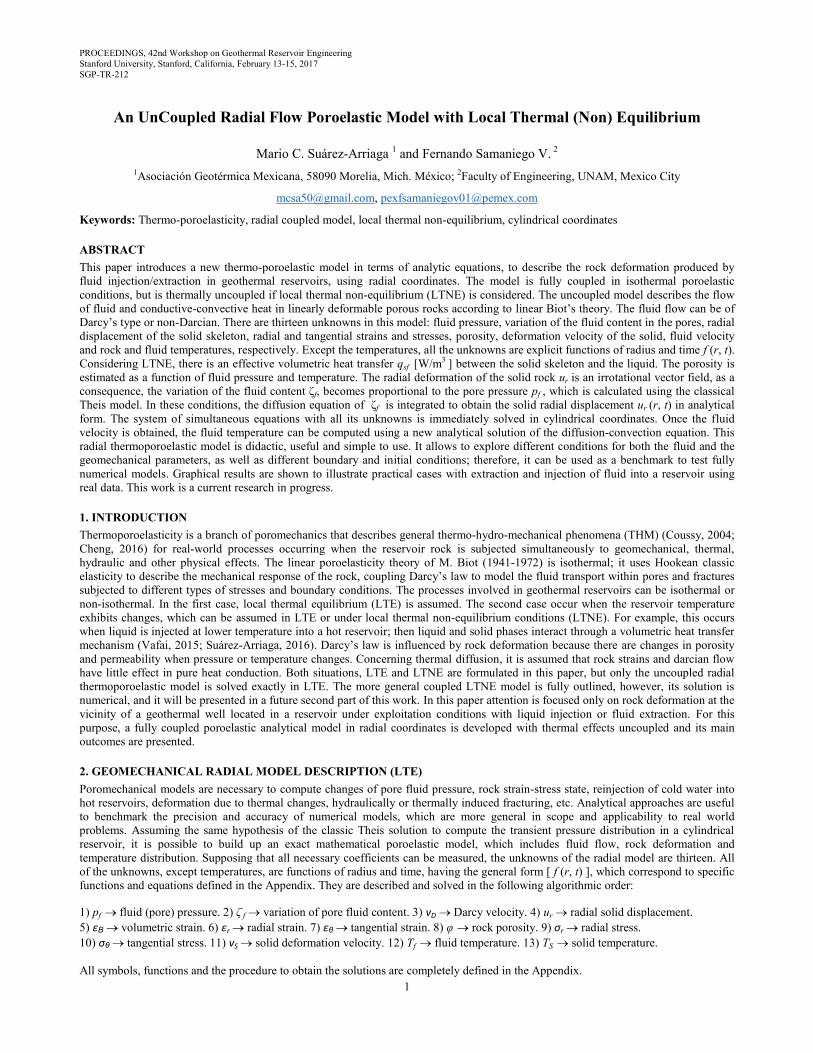
Figure 2: Fluid pressure (left) and radial Darcy velocity distribution (right) around the well, between 0.1 and 300 seconds.
a) b)
Suárez-Arriaga
4
Figure 3: Fluid content removal (left) and rock porosity reduction (right). Both simulation times are between [0.1, 3600] seconds
in order to observe the rapid initial poroelastic variations (reductions) produced by the fluid extraction.
Figure 4: Radial displacement of the solid skeleton (left) and rock velocity (right) between 0.1 and 3600 seconds. Both vectors
present negative values because the solid displacement occurs in the negative direction of the radial coordinate r.
Figure 5: Radial stress (left) and volumetric strain (right) of the poroelastic rock between 0.1 and 3600 seconds. The values of σr
correspond only to the extra stress (tension > 0) generated by the fluid extraction; the overburden pressure is about 300
bar. The strain εB < 0 because the solid displacements occur in the negative direction of the radial coordinates r and θ.
a)
b) a)
b)
a) b)
Suárez-Arriaga
5
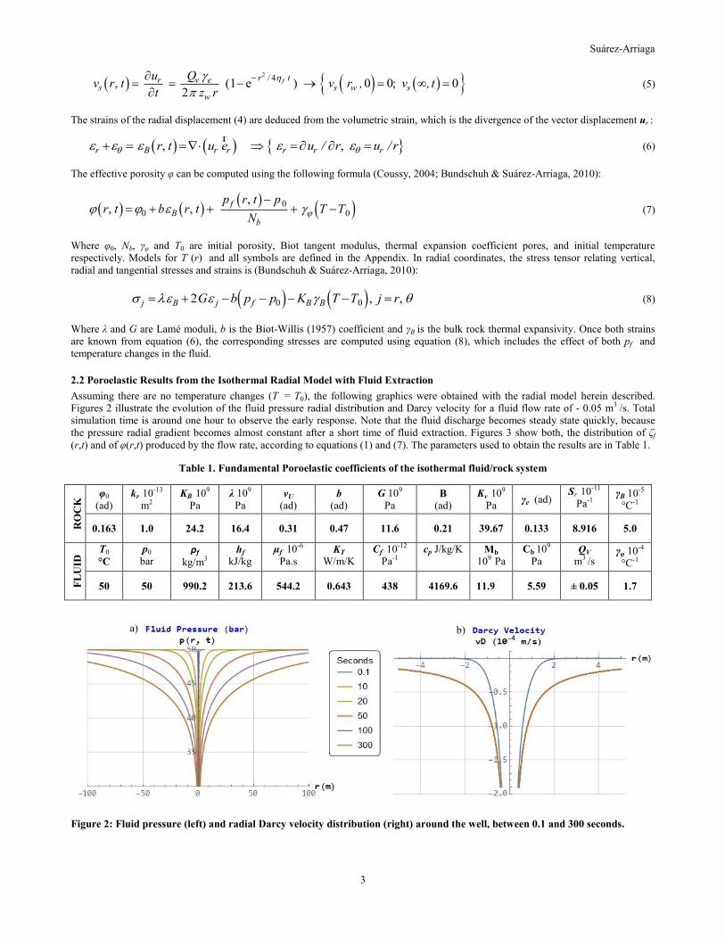
2.3 ThermoPoroelastic Results from the non-Isothermal Radial Model with Fluid Injection
If there are temperature differences (ΔT = 10°C) during fluid injection, it is necessary to add the effect of the thermal stress. Once both
strains are known (Eq. 6), stresses and porosity are computed using equations (7) and (8) to include the effect of both pressure and
temperature changes in the fluid/rock system. The following graphical results are obtained for an injection rate Qv = + 0.05 m3 /s:
Figure 6: Fluid pressure (left) and radial Darcy velocity distribution (right) around the well, between 0.1 and 3600 seconds.
Figure 7: Fluid content variation (left) and rock porosity increment (right). Simulation times are between [0.1, 3600] seconds.
Figure 8: Radial displacement of the solid skeleton (left) and rock velocity (right) between 0.1 and 3600 seconds. Both vectors
present positive values because the solid displacement occurs in the same direction of the radial coordinate r > 0 (Fig. 1).
b) a)
a) b)
b) a)
Suárez-Arriaga
6
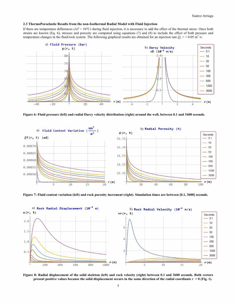
Figure 9: Radial (left) and tangential stress (right) in the poroelastic rock between 0.1 and 3600 seconds. The values of σr and σθ only represent the extra compression (< 0) generated by the fluid injection; the overburden pressure is about 300 bar.
Both stresses are negative because they correspond to compressions acting on the porous rock in both directions.
Figure 10: Radial (left) and tangential strain (right) of the poroelastic rock between 0.1 and 3600 seconds. Both strains are > 0
because the solid displacements occur in the positive direction of the radial coordinates r and θ.
Figure 11: Average stress ( [σr + σθ + σz ]/3, left) and volumetric strain (right) of the poroelastic rock between 0.1 and 3600
seconds. The values of σm correspond only to the extra compression in the rock generated by the fluid injection; the
overburden pressure is about 300 bar. The strain εB > 0 because the solid displacements occur in the positive direction of
the radial and tangential coordinates r and θ.
b) a)
a) b)
b) a)
Suárez-Arriaga
7
2.4 Brief Discussion of Graphical Results
The results obtained with the radial model, show and confirm several interesting experimental facts: first of all, fluid extraction or
injection in a well (Figs. 2 and 6) produces poroelastic deformations (Figs. 4a, 5b, 8a and 10a,b). Even if they are of small magnitude,
the strains and solid displacements are numerically detected at very early times, in the order of seconds (Figs. 4a, 5b, 8a, 10a,b and 11b).
This occurs because the liquid flows through a porous rock whose solid skeleton can be deformed elastically instantaneously. Fluid
extraction/injection in the reservoir causes the reduction/increment of the internal pore pressure (Figs. 2a and 6a) affecting both, the
liquid content and the effective porosity (Figs. 3 and 7). Their magnitude is proportional to the volumetric flow rate (Eq. 4). A wave of
non-negligible amplitude appears in the porous rock immediately after the fluid extraction/injection begins (Figs. 4b and 8b), but it is
rapidly attenuated during the next simulation times. Therefore, the presence of the moving fluid in the porous rock modifies its
mechanical response.
The internal tension produced by the liquid extraction (Fig. 5a), induces a decline of the fluid pressure and of the pore fluid content (Figs. 2a
and 3a). The corresponding reduction of effective porosity (Fig. 3b) can be the principal source of liquid released from storage. When the
poroelastic rock is subjected to internal compression because of injection (Figs. 6, 9 and 11a), the resulting matrix deformation leads to
a volumetric increase of the pores containing the fluid (Figs. 7a,b and 11b). This increment of the pore volume must be bounded by
physical poroelastic limits, defining a transitional zone before the rock enters the non-linear poroplastic region, where it can fail or be
fractured. A practical condition for fracturing is given by the following empirical formula:
frac IP t p t (9)
Where Pfrac is the minimum pressure for the fracture to occur, σθ is the previously defined tangential stress (Eq. 8 and Fig. 9b) and pI is
the extra pressure of the injected fluid. This breaking pressure depends on several factors, specifically on the injection rate.
3. ANALYTICAL SOLUTIONS FOR TEMPERATURES IN THE RADIAL MODEL (LTNE)
In a pseudo-stationary state (∂/∂t ~ 0) for the temperatures of the solid and liquid phases, a Local Thermal Non-Equilibrium uncoupled
radial model is obtained. Assuming that the temperature in the solid skeleton at r = rw is Tw, and at distance r = rL >> rw is TL, the
analytic solution for the solid temperature TS (r) in radial coordinates for these boundary conditions is (see Appendix):
2 2 2 2 2 24 4 4
4 /
S L w w L S S L L S w S w w S L
s
S w L
Q r r T T Ln r Q r r T Ln r Q r r T Ln rT r
Ln r r
(10)
Where Qs is the global solid heat transfer and δS is solid thermal diffusivity. The corresponding radial solution for the fluid temperature
is (see Appendix):
2
2
2
L Di f f D f w w D
f w
w Di f f D f L L D
f L
D Li f f D f L w L w D
f w
f
r v rE Q Ln v Q r r T v
r
r v rE Q Ln v Q r r T v
r
r v rE Q Ln v Q r r T T v
rT r
2 w D L DD i i
f f
r v r vv E E
(11)
Where Qf is the fluid heat transfer and δf is fluid thermal diffusivity; Tw = Tf (rw ) and TL = Tf (rL ) are the radial boundary conditions.
The special function Ei (x) = - E1 (- x) is another form of the classical exponential integral (Abramowitz & Stegun, 1972). Both
equations (10) and (11) are coupled by the volumetric heat transfer coefficient qsf :
2
, , , s s
s f s s f fss f S f
s s f f s s f f
q q q kkC mQ Q
c c c c
(12)
Where cs, cf are solid and fluid specific heat, ρs, ρf and ks, kf are solid and fluid thermal conductivities respectively. All these terms are
discussed in a previous paper (Suárez-Arriaga, 2016) and briefly redefined, in the Appendix.
The average temperature of the reservoir in pseudo-stationary state is:
Suárez-Arriaga
8
1 s fT r T r T r (13)
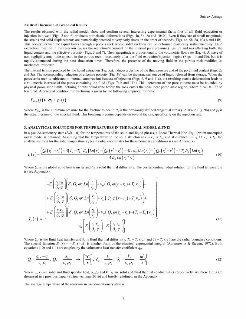
The corresponding graphics of both temperatures are:
Figure 12: Solid (left) and Fluid (right) temperatures as functions of the radial coordinate r. The values of the heat transfers are
Qs = 0.1 °C/s and Qf = 0.5 10-7 °C/s respectively; the Darcy velocity is vD = 0.7 10-8 m/s. Other data used are in Table 1.
Equations (11) and (13) are valid for any values of the fluid velocity, Darcian or non-Darcian. The pseudo-stationary state is only valid
for short injection times measured in minutes, or few hours. This approximation is not valid for larger residence times of the fluid.
4. CONCLUSIONS
Assuming the hypothesis of the classic Theis solution for pressure in a radial reservoir, an exact mathematical thermoporoelastic model
was constructed. This model includes fluid flow, rock deformation and temperatures distribution. The total number of unknowns of the
radial model are thirteen with the same number of equations. The results obtained show several interesting facts:
- The transport of a fluid in the reservoir modifies its mechanical response. Fluid extraction or injection in a well produces poroelastic
deformations. Even if they are of small magnitude, the strains and solid displacements are detected at very early times, in the order of
seconds, because the liquid flows through a porous rock whose solid skeleton can be deformed elastically in linear form.
- Fluid extraction or injection in the reservoir causes the reduction/increment of the pore pressure affecting both, the liquid content and
the effective porosity in direct proportion to the volumetric flow rate.
- A wave of non-negligible amplitude appears in the vicinity of the well immediately after the fluid extraction/injection begins. This
wave is rapidly attenuated.
- The internal tension produced by liquid extraction induces a decline of the fluid pressure and of the pore fluid content. There is a
corresponding reduction of porosity that can be the principal source of liquid released from storage.
- The internal compression produced by fluid injection, causes a skeleton deformation that leads to a volumetric increase of the pores
containing the fluid. This increment of porosity must be bounded by physical poroelastic limits, defining a transitional zone before the
poroplastic region appears, where the rock can be fractured.
- This model can be useful to explore the start of a hydraulic fracturing process. Unpublished experimental data show that during
a stimulation treatment performed in a low-permeability reservoir, which consisted in the injection of fluids at high pressure and flow
rate into the formation interval of interest, a vertical fracture of 2.7 cm aperture was created after 300 seconds of continuous injection.
The peak value of the injection pressure was 282 bar, which corresponded to the breaking pressure. After this peak, it was a pressure
draw-down, which was stabilized at 160 bars during the next 10 hours of continuous injection.
- It is well known that hydraulic fracturing can create high-conductivity paths within a large area of the reservoir. The
pressure increment caused by liquid injection induces the rock formation to fracture hydraulically. The breaking pressure required to
induce fractures in a rock at a given depth can be estimated with this radial model if the maximum poroelastic radial displacement of the
rock is known.
- This work is intended to explore the physical limits of a correct analytical solution of the thermoporoelastic problem in geothermal
reservoirs. All the unknowns were successfully coupled in the isothermal poroelastic case. However, under local thermal non-
equilibrium conditions the coupling is not possible using the exact model. The development of a numerical solution for the fully coupled
non-isothermal case is a current research work in progress.
Suárez-Arriaga
9
5. APPENDIX: CONSTRUCTION OF THE RADIAL MODEL
The basic equations governing the radial behavior of a linear thermoporoelastic rock are deduced from general principles and physical
laws well established (Biot, 1941, 1955, 1972; Wang, 2000; Coussy, 2004; Bundschuh & Suarez-Arriaga, 2010; Vafai, 2015; Cheng,
2016). The main general principle is the equilibrium equation in poroelasticity:
, 0T ix t σ (A0)
Where σT is the total stress tensor acting in the fluid-rock system. The strains in the solid skeleton are defined in terms of the
components of the vector displacement of solid particles u = ui (xi) ei :
1,
2
jii i j
j i
uux t
x x
ε (A1)
Where ε is the strain tensor and xi represents any kind of coordinate, Cartesian, radial, etc. The equation relating stresses and strains is:
0 02i j B i j i j f i j B B i jG b p p K T T (A2)
Where εB (= εxx + εyy + εzz ) is the volumetric strain, δij is the unit tensor, λ and G are the Lamé and shear coefficients respectively for
drained conditions, p0, T0 are the reservoir initial pore pressure and initial temperature, b is the Biot-Willis coefficient, KB is the bulk
modulus, and γB is the bulk thermal moduli; all coefficients are defined in the next section. Substituting equation (A2) into the
equilibrium condition (A0) and using equation (A1) we obtain the first governing linear thermoporoelastic formula:
2 2
30
fi i s
i jB B
iB
j j i
pu uG T
x x x x x xK G b K
(A3)
Using the law of mass conservation and Darcy’s law, the second governing equation for the fluid flow is obtained:
2
Bf f
B
i s
f f f
i
k bp p T
x x t tb b
K tK
(A4)
Under the most general conditions of local thermal non-equilibrium or LTNE state (Ts ≠ Tf ), the heat transfer process between phases is
modeled by the following two partial differential equations, one for the solid phase (s) and one for the fluid phase (f ):
3 1 1 1 1
ms s s s s s sf
Wc T T q q
t
k (A5)
3 mf f f f f f f f D sf
Wc T T c T v q
t
k (A6)
where t, φ, c, ρ, T, k, vD, qs and qsf are time, porosity, heat capacity, density, temperature, conductivity tensor, Darcy velocity and
volumetric heat generation of the solid (s) and fluid (f ) phases respectively. The symbol qsf is the amount of volumetric heat transferred
from the solid matrix to the fluid and viceversa (Vafai, 2015; Suárez-Arriaga, 2016); this term is a function of the solid-fluid
temperature difference (Ts - Tf ); the volumetric heat qsf depends also on a thermal coefficient and geometric variables. The microscopic
fluid velocity in the pores vf , is related to the Darcy flux vD by the Dupuit-Forchheimer relation vD = φ vf (Bear, 1973).
The general equations (A2, A3, A4, A5, A6) include the energy transfer between the solid and the fluid phases at different temperatures;
they correspond to a set of coupled equations governing general thermo-hydro-mechanical phenomena (THM) in porous rocks in LTNE.
The main unknowns are, the vector displacement of the solid particles u, the strain tensor ε, the fluid pressure pf and the fluid and rock
temperatures Tf and Ts respectively. However, this linear formulation corresponds to a partial thermally uncoupled model, because both
temperatures can be solved independently of the other unknowns if fluid velocity, porosity and initial and boundary conditions are
known.
5.1 The Basic Radial Equations
If only radial coordinates are considered, all variables involved in the isothermal radial model are functions of radius and time [ f (r,t) ].
In non-isothermal conditions, the rock and liquid temperatures can be obtained as analytic functions of the radius only in a pseudo-
stationary state. The vector displacement of the solid rock has only one component acting in the radial direction and, therefore its
rotational is zero (Figure 13). The total number of unknowns in the radial model are thirteen, they are solved in the following
algorithmic order:
Suárez-Arriaga
10
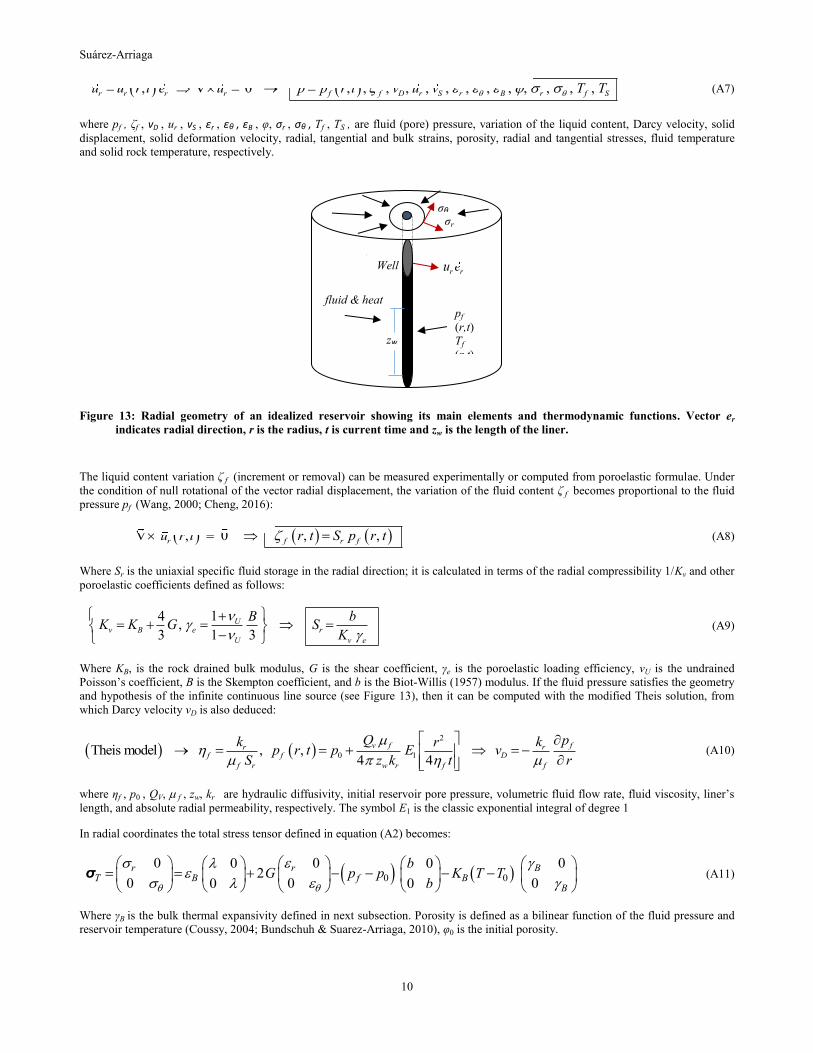
, 0 , , , , , , , , , , , , , r r r r f f D r S r B r f Su u r t e u p p r t v u v T T (A7)
where pf , ζf , vD , ur , vS , εr , εθ , εB , φ, σr , σθ , Tf , TS , are fluid (pore) pressure, variation of the liquid content, Darcy velocity, solid
displacement, solid deformation velocity, radial, tangential and bulk strains, porosity, radial and tangential stresses, fluid temperature
and solid rock temperature, respectively.
Figure 13: Radial geometry of an idealized reservoir showing its main elements and thermodynamic functions. Vector er
indicates radial direction, r is the radius, t is current time and zw is the length of the liner.
The liquid content variation ζ f (increment or removal) can be measured experimentally or computed from poroelastic formulae. Under
the condition of null rotational of the vector radial displacement, the variation of the fluid content ζ f becomes proportional to the fluid
pressure pf (Wang, 2000; Cheng, 2016):
, 0 , ,r f r fu r t r t S p r t (A8)
Where Sr is the uniaxial specific fluid storage in the radial direction; it is calculated in terms of the radial compressibility 1/Kv and other
poroelastic coefficients defined as follows:
14,
3 1 3U
v B e r
U v e
B bK K G S
K
(A9)
Where KB, is the rock drained bulk modulus, G is the shear coefficient, γe is the poroelastic loading efficiency, νU is the undrained
Poisson’s coefficient, B is the Skempton coefficient, and b is the Biot-Willis (1957) modulus. If the fluid pressure satisfies the geometry
and hypothesis of the infinite continuous line source (see Figure 13), then it can be computed with the modified Theis solution, from
which Darcy velocity vD is also deduced:
2
0 1Theis model , , 4 4
v frf f D
f r w r f
fr
f
Qk rp r t p E v
S z k
pk
t r
(A10)
where ηf , p0 , QV, f , zw, kr are hydraulic diffusivity, initial reservoir pore pressure, volumetric fluid flow rate, fluid viscosity, liner’s
length, and absolute radial permeability, respectively. The symbol E1 is the classic exponential integral of degree 1
In radial coordinates the total stress tensor defined in equation (A2) becomes:
0 0
0 0 02
0 0
0 0 00 0
r r BB f B
BT
bG p p K T T
b
σ (A11)
Where γB is the bulk thermal expansivity defined in next subsection. Porosity is defined as a bilinear function of the fluid pressure and
reservoir temperature (Coussy, 2004; Bundschuh & Suarez-Arriaga, 2010), φ0 is the initial porosity.
σr σθ
fluid & heat pf
(r,t)
Tf
(r,t)
ζf (r,t)
Well
zw
r ru e
Suárez-Arriaga
11
00 0,
fB
b
p pr t b T T
N
(A12)
Where Nb is the tangent Biot modulus, γφ is the thermal expansion coefficient of pores at constant pf and defined in next subsection.
Physically, any applied radial stress σr generates a strain εr producing simultaneously a perpendicular tangential strain εθ, which
corresponds to a tangential stress σθ (Figure 13). The strains of the radial displacement (A7) are deduced from the volumetric strain,
which is equal to the divergence of the vector displacement ur :
, , r r r rr B r r r
u u u ur t u e
r r r r
r (A13)
5.2 The Theis Model in the Diffusion Equation for the Fluid Content Variation
This classical Theis mathematical model has the following initial, internal and external boundary conditions that are also satisfied by ζf :
0
00
, , 0 , 0
external & internal boundaries: ,
2f f f f
f f f2
V ff
fr r
w w r
p p pp r, t > 0 = + p r, 0 = r t p
t r rr
Q p lim p r, t = lim = p
r 2 r z k
(A14)
The function ζf satisfies the same diffusion equation with appropriate initial and boundary conditions (Wang, 2000):
2
0 0
1, , 0 , 0, , ,
f
f f f w f
f
r t r t tt
(A15)
ζf also satisfies the following relationship in polar coordinates (Wang, 2000; Cheng, 2016):
0
1 , 0 0, 0, , , 0
f r
e r r r
r uu r u t U u t
r r r r
(A16)
γe is the coupled poroelastic coefficient defined in equation (A9), ηf is the hydraulic diffusivity defined in equation (A10) assumed to be
a function of the fluid temperature Tf only. The boundary and initial conditions in Eq. (A16) allows to integrate this equation exactly;
the corresponding integration constants are eliminated, because ur must be bounded for any value of (r, t ):
2
1 1 2
0
1, , , ,
2
rr e
e f e f r r f
r u rr t c t r r c t r u r t c t u r t r r t r
r r r
(A17)
The irrotational condition for the solid displacement, implies that the liquid content variation ζf is proportional to the fluid pressure pf ,
which can be computed with the Theis solution (Wang, 2000; Bundschuh & Suárez-Arriaga, 2010):
2 2
0 1 0 1, Theis model ,4 4 4 4
v f r v f
f f r
w f w f
Q S Qr rp r t p E r t S p E
z k t z k t
(A18)
The viscosity of liquid water grows slightly when pressure decreases, but its variability is larger when temperature changes. Therefore,
Theis model in equation (A18) can be used for every isothermal curve with fixed porosity, and is approximately valid when both
hydraulic diffusivity and porosity are updated for different fluid temperatures. It is interesting to mention here that S. Garg (1980)
derived a simple diffusivity equation for the two-phase flow of water in geothermal systems. His model is valid for reservoirs of radial
geometry with the same Theis’ hypothesis, which assume a fully penetrating well in a very large homogeneous, isotropic reservoir of
thickness zw. The main hypothesis in Garg’s model is that the reservoir is initially a two-phase system with uniform pressure and
temperature everywhere. The resulting two-phase partial differential equation and its solution are completely analogous to Eqs. (A15)
and (A18) for the liquid condition.
5.3 Computation of the Radial Displacement, Strains and Stresses
To obtain the solid radial displacement, the following procedure is used. The sudden injection of fluid at point (0, 0) is mathematically
equivalent to the classic problem of an instantaneous line source with injection of heat at time t = 0, which satisfies the same diffusion
Suárez-Arriaga
12
equation (A15) for ζf . The corresponding solution was obtained by Carslaw & Jaeger (1959, Chapter X, section 10.3) and is adapted
here for ζf with a fluid line source of strength q0:
2
40, 4
f
r
tp
f
f
qr t e
t
(A19)
Substituting this point source into equation (A16) the radial displacement corresponding to the sudden impulse produced in the solid
skeleton by the instantaneous fluid line source is obtained as:
2 2
4 40 0
0
, 14 2
f f
r rrt tp e e
r
f
q qu r t r e dr e
t r r
(A20)
The radial displacement produced by an infinite continuous line source, corresponding to the Theis solution, is obtained by integrating
equation (A20), replacing the value of the point source rate q0 by the volumetric flow rate per unit length Qv d t / zw:
2
24
0
021 e
8
4,
4fv e
rttfp
f
vr r
w w f
tQ ru r t u dt
z z r t
Q r
(A21)
Where Γ0 is the incomplete Gamma function of order 0, a special function defined for a ≥ 0 (Abramowitz & Stegun, 1972) as follows:
1[ ] a x
a
w
w x e d x
(A22)
The correctness of the solution given by equation (A21) can be verified calculating the partial derivative of ur (r, t) with respect to time
t:
2 2 2
24 4
0
401e 4 4 e
8, 1 ,
4 2f ff
r r
t
r
t pv e
f
er
t
r
Q qru r t e u r t
t t t rt rz
(A23)
Once the radial displacement ur is obtained from equation (A23), all the other unknowns can be computed directly with the relationships
given by equations (A11, A12 and A13) in the order indicated by equation (A7). Darcy and solid velocities are easily computed:
2
2
4
4
Theis model ,
,,
e2
1 e2
f
f
r
f vr
f
r
v e
w
t
D
w
tr
S
v r tz
u r t
p Qk
r r
Q
z rv r t
t
(A24)
5.3.1 Definitions of Experimental ThermoPoroelastic Coefficients
The coefficients introduced in previous equations are defined as follows. The variation of the fluid content ζf can be experimentally
measured as (Biot, 1941; Wang, 2000):
0
f ff f ,
(A25)
where ρf is fluid density, φ is current porosity and ρ0 is the initial fluid density. The thermal expansion coefficients, bulk modulus and
compressibilities are defined as follows:
1 1 1 1 1, , ,
f k
fsfB B
f Bs fp p f T
= KC
T T p CK
(A26)
Where Cf , CB , are fluid and bulk compressibilities respectively, and Kf is the bulk rock modulus. Biot moduli are defined next:
Suárez-Arriaga
13
01 1 1, , ,
fB B
f k
f f B b fp
p Vb C b M
M p p V N M K
(A27)
Detailed developments of all these moduli are described in (Bundschuh & Suárez-Arriaga, 2010 and Wang, 2000).
5.4 Analytical Solutions of Temperatures in the pseudo-Stationary LTNE Radial Model
Assuming a quasi-stationary state (∂/∂t ~ 0), equation (A5) in radial coordinates TS (r) becomes:
10 , ,
S S w wS SS
S LS s s
Q T r r TT kr
T r L Tr r r c
(A28)
Where ηS is the thermal diffusivity of the solid rock. Integrating twice, the analytic solution for this PDE is simply:
2 2 2 2 2 24 4 4
4 /
S L w w L S S L L S w S w w S L
s
S w L
Q r r T T Ln r Q r r T Ln r Q r r T Ln rT r
Ln r r
(A29)
Where QS (°C/s) is the global solid heat transfer and δS is its thermal diffusivity in geothermal rocks. The conduction-convection heat
partial differential equation equation for the liquid when the fluid flow is radial and quasi-stationary, with corresponding boundary
conditions is:
01, ,
f wff f fDf
f Lf f f f
T r r TQT T kvr
T r L Tr r r r c
(A30)
Where δf is the thermal diffusivity of the fluid. Integrating twice and replacing the constant boundary conditions, the solution of this
equation is:
2
0
2
2
0
L Di f f D f w D
f w
w Di f f D f L L D
f L
D Li f f D f L w L D
f w
f
r v rE Q Ln v Q r r T v
r
r v rE Q Ln v Q r r T v
r
r v rE Q Ln v Q r r T T v
rT r
2 w D L DD i i
f f
r v r vv E E
(A31)
Where Ei is another exponential integral defined as (Abramowitz & Stegun, 1972): x
i
w
eE w d x
x
.
The average temperature in the reservoir at any time in the pseudo-stationary state is:
1 s fT r T r T r (A32)
The previous equation is valid for typical values of the fluid velocity in pores and fractures and for short times measured in minutes or
hours. The pseudo-stationary approximation is not valid for long residence times of the fluid.
5.4.1 Computing the radial displacement as function of pressure and temperature
The differential equation of the radial rock displacement ur (r, t) is defined as (Bundschuh & Suárez-Arriaga, 2010):
Suárez-Arriaga
14
2
2 2
,4 10
3
f fr r rB B B
p r t T ru u uK G b K
r r r r r r
(A33)
Solving by a special mathematical technique, this equation accepts a very large analytical solution in the functional form of:
2
, , , , , , , , , , , ,4
r D f L w w L w v i
f
ru r t F v r r u T T Q r t E
t
(A34)
Where uw = ur (rw, 0); this solution is too large to include it here.
REFERENCES
Abramowitz, M. and Stegun, I.A. (eds): Handbook of mathematical functions with formulas, graphs, and mathematical tables. National
Bureau of Standards, Applied Mathematics Series 55, issued June 1964, tenth printing, December 1972, with corrections,
http://www.math.sfu.ca/~cbm /aands/ (accessed August 2009).
Biot, M.A.: General theory of three-dimensional consolidation. J. Appl. Physics 12 (1941), 155–164.
Biot, M.A.: Theory of elasticity and consolidation for a porous anisotropic solid. J. Appl. Physics 26 (1955), 182–185.
Biot, M.A.: Theory of finite deformations of porous solids. Indiana Univ. Math. J. 21:7 (1972), 597–620.
Biot, M.A. and Willis, D.G.: The elastic coefficients of the theory of consolidation. J. Appl. Mech. 24 (1957), 594–601.
Bundschuh, J. and Suarez-Arriaga, M.C.: Introduction to the Numerical Modeling of Groundwater and Geothermal Systems –
Fundamentals of mass, energy and solute transport in poroelastic rocks. Vol. 2, Multiphysics Modeling Series, CRC Press – Taylor
& Francis Group (2010).
Carslaw, H.S. and Jaeger, J.C.: Conduction of heat in solids. 2nd ed, Oxford Clarendon Press, Oxford, UK, (1959).
Cheng, A.H.D.: Poroelasticity, Theory and Applications of Transport in Porous Media Series Vol. 27, ed. Hassanizadeh, S.M. Founding
series editor: Jacob Bear, (2016), Springer Int. Pub., http://www.springer.com/series/6612/ .
Coussy, O.: Poro mechanics. John Wiley & Sons, New York, NY, (2004).
Garg, S.K.: Pressure transient analysis for two-phase (water/steam) geothermal reservoirs. Society of Petroleum Engineers Journal,
(1980), paper 7479, 206-214.
Suárez-Arriaga, M.C.: Local Thermal Non-Equilibrium Interfacial Interactions in Heterogeneous Reservoirs - Divergence of Numerical
Methods to Simulate the Fluid and Heat Flow, Proceedings, 40th Workshop on Geothermal Reservoir Engineering, Stanford
University, Stanford, CA (2016).
Vafai, K., (editor): Handbook of Porous Media, CRC Press – Taylor & Francis Group (2015).
Wang, H.F.: Theory of linear poroelasticity—with applications to geomechanics and hydrogeology. Princenton University Press, New Jersey, NJ, (2000).