+ All Categories
Home > Documents > A G eneric F ram ew ork for S ca lable a nd C onv ergent M ...stergios/papers/MED-2011.pdf · A G...

A G eneric F ram ew ork for S ca lable a nd C onv ergent M ...stergios/papers/MED-2011.pdf · A G...

Date post: 29-Sep-2018
Category:
Upload: vanhanh
View: 213 times
Download: 0 times
Share this document with a friend
6
A Generic Framework for Scalable and Convergent Multi-Robot Active Simultaneous Localization, Mapping and Target Tracking E.B. Kosmatopoulos, D.V. Rovas, L. Doitsidis, K. Aboudolas, and S.I. Roumeliotis Abstract— In this paper, a new approach is proposed and analyzed for developing efficient and scalable methodologies for multi-robot active Cooperative Simultaneous Localization And Mapping and Target Tracking (C-SLAMTT). The proposed approach employs an active estimation scheme that switches among linear elements and, as a result, its computational requirements scale linearly with the number of estimated quan- tities (number of number of robots, landmarks and targets). The parameters of the proposed scheme are calculated off-line using a convex optimization algorithm which is based on Semi- Definite Programming (SDP) and approximation using Sum-of- Squares (SoS) polynomials. As shown by rigorous arguments, the estimation accuracy of the proposed scheme is equal to the optimal estimation accuracy plus a term that is inversely proportional to the number of estimator’s switching elements (or, equivalently, to the memory storage capacity of the robots’ equipment). The proposed approach can handle various types of constraints such as “stay-within-an-area”, obstacle avoidance and maximum speed constraints. The efficiency of the approach is demonstrated on a 3D active cooperative simultaneous map- ping and target tracking application employing flying robots. I. I NTRODUCTION The majority of techniques and methods for multi-robot sensing and estimation applications are based on local approximations of the overall system dynamics (team of robots + measurement model + the external environment): for instance, in Passive Sensing (PS) applications such as passive target tracking, localization, mapping, Cooperative Simultaneous Localization And Mapping (C-SLAM), etc, the majority of existing approaches employ Extended Kalman Filter (EKF) or similar techniques which are based on lin- earization of the overall system dynamics, see e.g., [16], [13], [2]. A similar situation is also present in Active Sensing (AS) applications such as active target tracking, active C-SLAM, etc, where the objective is to generate the robots’ trajectories E.B. Kosmatopoulos is with the Dept. of Electrical and Computer Engineering, Democritus University of Thrace, Xanthi 67100, Greece and the Informatics & Telematics Institute, Center for Research and Technology–Hellas (ITI-CERTH), 6th km Xarilaou - Thermi, 57001, Thessaloniki, Greece, (e-mail: [email protected]). D.V. Rovas is with the Dept. of Production & Management Engineering, Technical University of Crete, Chania, 73100, Greece and the Informatics & Telematics Institute, Center for Research and Technology–Hellas (ITI-CERTH), 6th km Xarilaou - Thermi, 57001, Thessaloniki, Greece, (e-mail: [email protected]). L. Doitsidis is with the Dept. of Electronics, Technological Educational Institute of Crete, Chania, 73100, Greece and the Informatics & Telematics Institute, Center for Research and Technology–Hellas (ITI-CERTH), 6th km Xarilaou - Thermi, 57001, Thessaloniki, Greece, (e-mail: [email protected]). K. Aboudolas is with the Informatics & Telematics Institute, Center for Research and Technology–Hellas (ITI-CERTH), 6th km Xarilaou - Thermi, 57001, Thessaloniki, Greece, (e-mail: [email protected]). S.I. Roumeliotis is with Dept. of Computer Science and Engineering University of Minnesota EE/CS 5-189, 200 Union St. SE Minneapolis, MN 55455, (e-mail: [email protected]). The research leading to these results has received funding from the European Commission FP7-ICT Cognitive Systems, Interaction, and Robotics under the contracts #231855 (sFLY) and #270180 (NOPTILUS). so that estimation accuracy is optimized. In most of the exist- ing approaches, the trajectory generators are usually based on convex or local approximations (relaxations) of non-convex optimization problems, see e.g., [16], [5], [14]. However, linearization (in case of PS) or relaxation (in case of AS) may have a significant or even devastating effect on the overall system efficiency due to e.g., estimator divergence or convergence to local minima. Attempts that have been made to employ techniques that avoid the usage of linearization or convex/local relaxations face the well-known problem of curse of dimensionality: for instance, the algorithms of [3], [12], [5], [11], [14], require the implementation of algorithms that scale poorly with the number of the robot team members and, as a result, their deployment in large-scale, real-life applications is formidable and/or they cannot guarantee of efficient and convergent performance. In this paper, we propose and analyze a new approach that overcomes the above mentioned shortcomings. The proposed approach adopts a general framework that can treat in a uni- fied manner a large class of multi-robot AS applications such as active target target tracking, localization, active SLAM or any combinations of them. Contrary to the approaches that are based on linearization or local approximation/relaxation, the proposed approach uses the full nonlinear model of the overall multi-robot system dynamics in order to construct an estimator/trajectory generator that fulfills the computational and other physically-imposed requirements imposed by the particular multi-robot application. Moreover, it guarantees aribtrary-close-to-optimal, convergent and efficient perfor- mance of the overall estimation process. Due to space limitations the proof of our theoretical results are omitted and will be reported elsewhere. A. Notations & Preliminaries xis used to denote the standard Euclidean norm of the vector x. For a symmetric matrix A, the notation A 0 (A 0) is used to denote that A is a positive definite (resp. positive semidefinite) matrix. dim(x) denotes the dimension of the vector x. I n denotes the n × n identity matrix. For a smooth function V (x 1 ,x 2 ) where x i are vectors, the following notation is used: V xi (x 1 ,x 2 )= ∂V ∂xi (x 1 ,x 2 ), V xixi (x 1 ,x 2 )= 2 V ∂x 2 i (x 1 ,x 2 ). The following definition will be finally needed in the paper. Definition 1: Fix the positive integer L and let the vector x ∈ℜ n satisfy x‖≤ C for some positive constant C; the notation β(x)= B L n (x) will be used to denote the vector β(x)=[β 1 (x)x τ ,...,β L (x)x τ ] τ where β i are L smooth activation functions satisfying β i (x) [0, 1], L i=1 β i (x)= 19th Mediterranean Conference on Control and Automation Aquis Corfu Holiday Palace, Corfu, Greece June 20-23, 2011 TuBT1.1 978-1-4577-0123-8/11/$26.00 ©2011 IEEE 151
Transcript

A Generic Framework for Scalable and Convergent Multi-Robot

Active Simultaneous Localization, Mapping and Target Tracking

E.B. Kosmatopoulos, D.V. Rovas, L. Doitsidis, K. Aboudolas, and S.I. Roumeliotis

Abstract— In this paper, a new approach is proposed andanalyzed for developing efficient and scalable methodologies formulti-robot active Cooperative Simultaneous Localization AndMapping and Target Tracking (C-SLAMTT). The proposedapproach employs an active estimation scheme that switchesamong linear elements and, as a result, its computationalrequirements scale linearly with the number of estimated quan-tities (number of number of robots, landmarks and targets).The parameters of the proposed scheme are calculated off-lineusing a convex optimization algorithm which is based on Semi-Definite Programming (SDP) and approximation using Sum-of-Squares (SoS) polynomials. As shown by rigorous arguments,the estimation accuracy of the proposed scheme is equal tothe optimal estimation accuracy plus a term that is inverselyproportional to the number of estimator’s switching elements(or, equivalently, to the memory storage capacity of the robots’equipment). The proposed approach can handle various typesof constraints such as “stay-within-an-area”, obstacle avoidanceand maximum speed constraints. The efficiency of the approachis demonstrated on a 3D active cooperative simultaneous map-ping and target tracking application employing flying robots.

I. INTRODUCTION

The majority of techniques and methods for multi-robot

sensing and estimation applications are based on local

approximations of the overall system dynamics (team of

robots + measurement model + the external environment):

for instance, in Passive Sensing (PS) applications such as

passive target tracking, localization, mapping, Cooperative

Simultaneous Localization And Mapping (C-SLAM), etc, the

majority of existing approaches employ Extended Kalman

Filter (EKF) or similar techniques which are based on lin-

earization of the overall system dynamics, see e.g., [16], [13],

[2]. A similar situation is also present in Active Sensing (AS)

applications such as active target tracking, active C-SLAM,

etc, where the objective is to generate the robots’ trajectories

E.B. Kosmatopoulos is with the Dept. of Electrical and Computer Engineering,

Democritus University of Thrace, Xanthi 67100, Greece and the Informatics &

Telematics Institute, Center for Research and Technology–Hellas (ITI-CERTH), 6th

km Xarilaou - Thermi, 57001, Thessaloniki, Greece, (e-mail: [email protected]).

D.V. Rovas is with the Dept. of Production & Management Engineering, Technical

University of Crete, Chania, 73100, Greece and the Informatics & Telematics Institute,

Center for Research and Technology–Hellas (ITI-CERTH), 6th km Xarilaou - Thermi,

57001, Thessaloniki, Greece, (e-mail: [email protected]).

L. Doitsidis is with the Dept. of Electronics, Technological Educational Institute

of Crete, Chania, 73100, Greece and the Informatics & Telematics Institute, Center

for Research and Technology–Hellas (ITI-CERTH), 6th km Xarilaou - Thermi, 57001,

Thessaloniki, Greece, (e-mail: [email protected]).

K. Aboudolas is with the Informatics & Telematics Institute, Center for Research

and Technology–Hellas (ITI-CERTH), 6th km Xarilaou - Thermi, 57001, Thessaloniki,

Greece, (e-mail: [email protected]).

S.I. Roumeliotis is with Dept. of Computer Science and Engineering University

of Minnesota EE/CS 5-189, 200 Union St. SE Minneapolis, MN 55455, (e-mail:

[email protected]).

The research leading to these results has received funding from the European

Commission FP7-ICT Cognitive Systems, Interaction, and Robotics under the contracts

#231855 (sFLY) and #270180 (NOPTILUS).

so that estimation accuracy is optimized. In most of the exist-

ing approaches, the trajectory generators are usually based on

convex or local approximations (relaxations) of non-convex

optimization problems, see e.g., [16], [5], [14]. However,

linearization (in case of PS) or relaxation (in case of AS)

may have a significant or even devastating effect on the

overall system efficiency due to e.g., estimator divergence or

convergence to local minima. Attempts that have been made

to employ techniques that avoid the usage of linearization

or convex/local relaxations face the well-known problem of

curse of dimensionality: for instance, the algorithms of [3],

[12], [5], [11], [14], require the implementation of algorithms

that scale poorly with the number of the robot team members

and, as a result, their deployment in large-scale, real-life

applications is formidable and/or they cannot guarantee of

efficient and convergent performance.

In this paper, we propose and analyze a new approach that

overcomes the above mentioned shortcomings. The proposed

approach adopts a general framework that can treat in a uni-

fied manner a large class of multi-robot AS applications such

as active target target tracking, localization, active SLAM or

any combinations of them. Contrary to the approaches that

are based on linearization or local approximation/relaxation,

the proposed approach uses the full nonlinear model of the

overall multi-robot system dynamics in order to construct an

estimator/trajectory generator that fulfills the computational

and other physically-imposed requirements imposed by the

particular multi-robot application. Moreover, it guarantees

aribtrary-close-to-optimal, convergent and efficient perfor-

mance of the overall estimation process.

Due to space limitations the proof of our theoretical results

are omitted and will be reported elsewhere.

A. Notations & Preliminaries

‖x‖ is used to denote the standard Euclidean norm of the

vector x. For a symmetric matrix A, the notation A ≻ 0(A � 0) is used to denote that A is a positive definite (resp.

positive semidefinite) matrix. dim(x) denotes the dimension

of the vector x. In denotes the n × n identity matrix.

For a smooth function V (x1, x2) where xi are vectors,

the following notation is used: Vxi(x1, x2) = ∂V

∂xi(x1, x2),

Vxixi(x1, x2) =

∂2V∂x2

i

(x1, x2). The following definition will

be finally needed in the paper.

Definition 1: Fix the positive integer L and let the vector

x ∈ ℜn satisfy ‖x‖ ≤ C for some positive constant C; the

notation β(x) = BLn (x) will be used to denote the vector

β(x) = [β1(x)xτ , . . . , βL(x)x

τ ]τ where βi are L smooth

activation functions satisfying βi(x) ∈ [0, 1],∑L

i=1 βi(x) =

19th Mediterranean Conference on Control and AutomationAquis Corfu Holiday Palace, Corfu, GreeceJune 20-23, 2011

TuBT1.1

978-1-4577-0123-8/11/$26.00 ©2011 IEEE 151

1,∑L

i=1 I (βi(x)) ≤ 2 where I(y) denotes the indicator

function I(y) = 1 if y > 0 and I(y) = 0 if y = 0.

II. MULTI-ROBOT ACTIVE SENSING SET-UP

We consider a team of NR robots deployed on a 2Dor a 3D environment containing NL static landmarks and

NT moving targets. For simplicity and to avoid unnecessary

lenghty formulas, we assume that a low-level controller (fast

inner control-loop) is implemented to each of the robots, so

that the velocity of each of the robots (after the application

of the low-level control) can be directly controlled. More-

over we assume that the target’s dynamics are reproduced

according to a zero-acceleration model, see e.g., [16]. Under

these assumptions the dynamics of the overall system can

be described according to the following set of differential

equations:

xR = BRu, xR(0) is known

xT = BTωT , xT (0), xT (0) are unknown

xL = 0, xL(0) is unknown

(2.1)

where xR denotes the vector of positions/poses of all NR

robots, u denotes the vector of all robots’ control inputs,

xT denotes the vector of positions of all NT targets and

xL is the (static) vector of all NL landmarks; BR and

BT are constant diagonal matrices and ωT denotes a zero-

mean unity-variance Gaussian random vector that drives the

targets. Note that by defining the augmented state vector as

x = [xτR, xτT , x

τT , x

τL]

τ, we can rewrite the overall system

dynamics according to

˙x = Bu+ BωωT (2.2)

for some appropriately defined constant matrices B and Bω.

We will further assume that the robots use proprioceptive

measurements (e.g., from odometric or inertial sensors) to

propagate their position or pose (position and orientation)

estimates, and are equipped with exteroceptive sensors (e.g.,

laser range finders, cameras, etc) that provide nonlinear

measurements (e.g., distance or bearing) of robot-to-robot,

robot-to-landmark and/or robot-to-target relative positions.

Let y denote the vector of all sensor measurements and

assume that these measurements are related to the system

(2.2) states according to

y = h(x, ξ) (2.3)

where h is a nonlinear vector function and ξ denotes the

sensor noise vector. We will assume that h is a differentiable

function (or that it can be approximated with arbitrary

accuracy by a differentiable function). A final assumption

is that the sensor noise is generated according to a colored

noise model, i.e.,

ξ = −aξ + ωS (2.4)

where a is a positive scalar and ωS is a zero-mean unity-

variance Gaussian random vector.

By defining χ = [xτ , ξτ ]τ and ω = [ωτT , ω

τS]

τ , we

can rewrite equations (2.2), (2.3), (2.4) into the following

compact form

χ = Aχ+Bu+Bωωy = h(χ)

(2.5)

where h(χ) ≡ h(x, ξ) and A,B,Bω are constant matrices

that depend on BR, BT and a.

The task the multi-robot team is called to accomplish is

that of active Cooperative Simultaneous Localization And

Mapping and Target Tracking – (active C-SLAMTT), i.e., the

problem of

• use the sensor signals y(t) in order to provide estimates

of the overall state vector χ(t),• while designing on-line the robot control signals u(t) so

that the overall estimation accuracy is maximized (i.e., the

robots are moving so that they “capture” as much information

as possible) and, moreover, the robot trajectories satisfy

physically-imposed constraints such as maximum height,

obstacle-avoidance, maximum speed, etc, constraints.

We close this section by noticing that there are two types

of physically-imposed constraints treated in this paper:

• Constraints that can be written in the form:

S(y) ≤ 0 (2.6)

where S can be any nonlinear vector function of the sensor

measurements y. Obstacle avoidance, maximum allowable

height constraints as well as constraints restricting the robots

to remain within an area can be written in the form (2.6).

• Control-related physical constraints such as that the control

inputs or the robot speeds should not exceed certain bounds.

Please note that these constraints cannot be written in the

form (2.6).

III. AS ESTIMATOR DESIGN

Having formulated the AS design problem for the active

C-SLAMTT case treated in this paper, we now proceed to

the proposed solution to this problem. The proposed solution

employs an estimator of the form

˙χ = Bu+ uoy = h(χ)

(3.1)

where uo is the correction vector. In this way the AS design

problem is transformed to the problem of designing on-line

the signals u and uo.

Assuming that the estimator (3.1) is employed, the optimal

AS estimator design can be formulated as a stochastic

optimal control problem described according1 to

min(u(s),uo(s),s∈[0,∞))

J (3.2)

J = J(χ(0), χ(0))

= E

[∫

0

(

‖χ(s)‖2 + ‖π(y(s))‖2)

ds

]

(3.3)

1For the time-being only the case of constraints of the type (2.6)is considered. For the extension to the case of control-related physicalconstraints see the end of this section. Also, the proposed approach canbe easily extended to cases where other optimization criteria than (3.3) areemployed.

978-1-4577-0123-8/11/$26.00 ©2011 IEEE 152

where χ(t) = χ(t)− χ(t) denotes the state estimation error,

π(y(s)) = vec(πi(y)), πi(y) = exp(αSi(y)−η), α is a large

positive constant and η is a positive constant chosen so that

if a particular constraint Si(y) ≤ 0 is – or is about to be –

violated, then the respective πi(y) takes a very large value,

while it is negligible when the constraint is satisfied.

Using the concepts of input/output representations and

filtering techniques it can be seen [6] that a possible math-

ematical description for the optimal u∗, u∗o (minimizing J )

is as follows

u∗(t) = kc(Y )

u∗o(t) = ko(Y ), Y =

[

y

Yf

]

(3.4)

for some unknown functions kc, ko, where

y =

[

yy

]

[

y − h(χ)y

]

, Yf =

1Λ(s) y

...1

Λp−1(s) y

and Λ(s) = (s+ ρ), with ρ being a positive design constant

and p being the smaller positive integer satisfying p ≥dim(χ)/dim(y).

By adopting a stochastic dynamic programming frame-

work, we let V denote the optimal-cost-to-go function, seee.g., [15], defined according to

V (X(t)) = min J(X(t)) (3.5)

J(X(t)) = E

[∫

t

(

‖χ(s)‖2 + ‖π(y(s))‖2)

ds

]

X =[

(χ− χ)τ , χτ , Y τf

]

By direct application of the Hamilton-Jacobi-Bellman equa-

tion, see e.g., [15], we obtain that the optimal-cost-to-go

function V satisfies

LV (X)

u(t)=u∗(t),uo(t)=u∗

o(t)

= −(

‖χ‖2 + ‖π(y)‖2)

(3.6)

where L stands for the Ito infinitesimal2 operator (generator)

acting on V (χ, χ) along the trajectories of (2.5) and (3.1),

see e.g., [4], and u∗, u∗o denotes the optimal values for the

signals u and uo, respectively.

In order to have a well-posed problem, we will assume that

the problem at hand admits a solution, or, equivalently that

the optimal-cost-to-go function and the associated optimal

signals u∗, u∗o satisfy the following assumption.

(A1) For all admissible initial conditions, the optimization

problem (3.5) – or, equivalently, the associated HJB equation

– admits a unique viscosity solution V satisfying V (X) = V0if χ = χ and V (X) > 0 if χ 6= χ, where V0 is a non-negative

constant.

Assumption (A1) requires that the problem at hand makes

sense, i.e., that for all admissible χ(0), χ(0), there exists a

control strategy u∗(t) that satisfies the constraints (2.6) and

renders system (2.5) stochastically observable. To keep our

analysis simple and avoid unnecessary technicalities, we will

assume hereafter that V0 = 0. All the results of this paper

2In simple words, L denotes the mean of the time-derivative of V (χ, χ)along the trajectories of (2.5) and (3.1).

can be readily extended to the case where V0 > 0, in which

case the term V0 should be added to the RHS of inequalities

(3.8) and (3.22) presented below.

By using the Ito formula [4] and (3.4), the HJB equation

(3.6) becomes

−(

‖χ‖2 + ‖π(y)‖2)

=

V τχ

(

Aχ+Bkc(Y ))

+ V τχ

(

Bkc(Y ) + ko(Y ))

+ V τ

Yf

(

Af Yf + Bf y)

+1

2tr

{

BτωVχχBω

}

(3.7)

The following lemma will be proven useful for comparing

the performance of the proposed AS scheme with that of the

optimal one.

Lemma 1: Let (A1) hold. Let also the following design

assumption hold:

(A2) The function S(y) in (2.6) is designed so that it

incorporates constraints that force the robots to remain within

a prespecified area [xmin, xmax, ymin, ymax, zmin, zmax].Then the optimal AS estimator, i.e., the AS estimator (3.1),

(3.4) satisfies

E

[

|χ(t)|2

]

≤ λ∗1e−λ∗

2t[

|χ(0)|2]

(3.8)

where λ∗i , i = 1, 2 are positive constants that depend on

(2.5) and (2.6).Let us now turn our attention to the proposed approach.

The first step in our approach is to employ standard approxi-

mators for approximating the functions V , kc and ko in (3.7).More precisely, consider the vectors ψ =

[

yτπ(y)τ]τ

,

ζ =[ √

β1(Y )(χ− χ)τ , . . . ,√

βL(Y )(χ− χ)τ , χτ , ψτ Y τ]τ

where β1(Y ), . . . , βL)(Y ) denote L activation smooth func-

tions satisfying Definition 1, i.e.,

β(Y ) =[

β1(Y ), . . . , βL(Y )]τ

= BL

dim(Y )(Y ) (3.9)

Then, V , kc and ko can be approximated (with an approxi-

mation accuracy that is inversely proportional to the number

L of activation functions) as follows:

V (X) ≈ ζτPζ

kc(Y ) ≈ κc(Y )Gcψ, ko(Y ) ≈ κo(Y )Goψ(3.10)

where κc(Y ) =[

β1(Y )Idim(u), . . . , βL(Y )Idim(u)

]

,

κo(Y ) =[

β1(Y )Idim(χ), . . . , βL(Y )Idim(χ)

]

and P,

Gc, Go are constant unknown matrices of appropriatedimensions. Using assumption (A1) and similar argumentsas those of [7]-[10], it can be seen that the matrix P ispositive definite and symmetric and assumes the followingblock diagonal form

P =

P1 0 0 0 0 0

0. . . 0 0 0 0

0 . . . PL 0 0 00 . . . 0 pIdim(χ) 0 00 . . . 0 0 pIdim(ψ) 00 . . . 0 0 0 pIdim(Y )

where Pi are dim(χ)2-dimensional symmetric and positive

definite matrices and p is a positive constant. Returning

978-1-4577-0123-8/11/$26.00 ©2011 IEEE 153

back to the definition of the vector ζ, it is not difficult for

someone to see that the terms ‖χ‖2 + ‖π(y)‖2, χ and ψ can

be rewritten as follows:

‖χ‖2 + ‖π(y)‖2 = ζτQζ (3.11)

ψ = Hζ, χ = Hζ, Y = ¯Hζ

By using (3.10) and (3.11), we have that the HJB equation

(3.7) can be rewritten – after some lengthy but straightfor-

ward manipulations – as follows

ν +O (‖P‖) = ζτ{

Q+Pζχ

(

AH +Bκc(Y )GcH)

+(

AH +Bκc(Y )GcH)τ

ζτχP

+Pζχ

(

Bκc(Y )GcH + κo(Y )GoH)

+(

Bκc(Y )GcH + κo(Y )GoH)τ

ζτχP

+PζY

(

Af¯H)

+(

Af¯H)τ

ζτYP}

ζ (3.12)

≡ ζτP (P,Gc,Go) ζ (3.13)

where Af is a constant matrix that corresponds on the state-

space realization of Yf and ν stands for the approximation

error term that is present due to the approximations (3.10)

and is inversely proportional to the number L of activation

functions. Equation (3.13) indicates that the problem of

constructing an approximately optimal AS performance can

be cast as the following optimization problem:

min[

‖ζτP (P,Gc,Go) ζ‖2 + ‖P‖

]

(3.14)

s.t. P ≻ 0

Unfortunately, as the term P(·) is a nonlinear function of

P,Gc,Go, attempting to solve (3.14) is a non-convex – and

thus difficult to be solved – problem. To circumvent this

problem we work similarly to [7]-[10]: by multiplying from

the left and the right the term P by P−1 we obtain that

ζτP−1P (P,Gc,Go)P−1ζ =

ζτ{

Q+ ζχ

(

AHP+Bκc(Y )FcH)

+(

PAH +Bκc(Y )FcH)τ

ζτχ

+ ζχ

(

Bκc(Y )FcH + κo(Y )FoH)

+(

Bκc(Y )FcH + κo(Y )FoH)τ

ζτχ

+ ζY

(

Af¯H)

P+ P(

Af¯H)τ

ζτY

}

ζ

= FP,Q,Fc,Fo

(χ, χ, Y ) (3.15)

where

P = P−1, Q = P−1QP−1 ≡ PQP (3.16)

and Fc,Fo denote two constant matrices satisfying

FcH = GcHP, FoH = GoHP (3.17)

The following lemma establishes that – in the case where

ν is negligible – solving the non-convex problem (3.14)

is equivalent to a convex problem related to the function

FP,Q,Fc,Fo

defined above.

Lemma 2: Consider the following optimization problem:

min[

‖FP,Q,Fc,Fo(χ, χ, Y )‖2 + tr (X)

]

(3.18)

s.t.

ǫ1I � P � ǫ2I, ǫ3Q � Q, 0 � Z, Z =

[

P II X

]

where ǫi, i = 1, 2, 3 are some positive design constants (withǫ2 > ǫ1) and X is a diagonal matrix. Let also G∗

c ,G∗

o,P∗

denote the optimal solutions to the optimization problem(3.14), P∗, Q∗,F∗

c ,F∗

o denote the optimal solutions to theoptimization problem (3.18) and

P⋆⋆ =(

P∗)−1

, G⋆⋆c = F∗

cH(

HP∗)H

, G⋆⋆o = F∗

oH(

HP∗)H

whereAH denotes the pseudo-inverse of the matrix A. Then,if the positive constants ǫi are chosen so that ǫ1I � P∗−1 �ǫ2I, ǫ3Q � P∗−1QP∗−1 we have that

P⋆⋆ = P⋆ +O(ν), G⋆⋆c = G⋆

c +O(ν), G⋆⋆o = G⋆

o +O(ν),

However the solution of the optimization problem (3.18)

requires discretization of the state-space as it is an infinite-

dimensional, state-dependent problem. Fortunately, due to

the particular form of the optimization problem (3.18), the

number of discretization points does not have to be as

large as it is required in a typical state-dependent opti-

mization problem: as it was seen in [7], [8] the number

of discretization points can be as few as the total number

of free variables in the matrices P, Q,Fc,Fo. This is in

contrary to alternative approaches that impose approximation

schemes for constructing estimation designs: for instance,

dynamic programming-based schemes require an extremely

larger number of discretization points.

Table I presents the proposed procedure for solving the

optimization problem (3.18) and, eventually, constructing the

proposed AS scheme. Following the same methodology as in

[7], [8], the key idea of the approach in Table I for solving

(3.18) is to choose randomly many different3 triplets x, x, Y ;

it suffices to choose the number of random triplets to be equal

or larger than the number of free variables in the matrices

P,Gc,Go. The next theorem establishes the properties of

the overall scheme presented in Table I.

Theorem 1: Fix the number L of activation functions

and the constants ǫi, i = 1, 2, 3 and let P, Q,Fc,Fo be

constructed according to the design procedure of Table I. Let

also (A1), (A2) hold. Then, the following statements hold:(a) If the following holds for some positive constant C1:

‖χ[i] − χ[i]‖2 > C1 ⇒ (3.21)

FP,Q,Fc,Fo(χ[i]

, χ[i], Y

[i])− ζτ (χ[i]

, χ[i])Qζ(χ[i]

, χ[i]) < 0

then

E

[

|χ(t)|2]

≤ λ1e−λ2t

[

|χ(0)|2]

+ λ3 (3.22)

where λi > 0 and, moreover, λ1 = λ∗1 + O(

1L

)

, λ2 =λ∗2 −O

(

1L

)

and λ3 ≡ C1 = O(

1L

)

.

3Please note that all the terms ζx, ζx, κc(Y ), κo(Y ) in (3.18) are

functions of χ, χ and Y .

978-1-4577-0123-8/11/$26.00 ©2011 IEEE 154

Table I: Proposed AS design approach

Step 1. Calculate the matrices P, Q,Fc,Fo as follows: Let N denote the total number of free variables of these matrices. Select randomly N points

χ[i], χ[i], Y [i], where N is any integer satisfying N ≥ N and solve the following convex optimization problem (here ǫi are user-defined positive constants):

min

[

N∑

i=1

‖FP,Q,Fc,Fo(χ[i]

, χ[i], Y

[i])‖2 + tr (X)

]

(3.19)

s.t.

ǫ1I � P � ǫ2I, ǫ3Q � Q, 0 � Z

Z =

[

P II X

]

Step 2. By using the solution of the above optimization problem, we can extract the matrices P,Gc,Go according to

P = P−1, Gc = FcH(

HP−1)H

, Go = FoH(

HP−1)H

(3.20)

Step 3. The proposed AS scheme is given by equations (3.1), (3.10).

(b) Assume additionally that the design constants ǫi satisfy

ǫ1I � P∗−1 � ǫ2I, ǫ3Q � P∗−1QP∗−1 where P∗

corresponds to the optimal value for the matrix P with

respect to the optimization problem (3.14). Then, for each

positive constant C1, there exists a lower bound L on the

number L of activation functions so that (3.21) holds for all

choices for L satisfying L ≥ L.

Furthermore to Theorem 1 and by using the same arguments

as those of [7],[10] it can be seen that, in case (3.21) holds,

then the solutions of the overall system satisfy the following

inequality:

|ζ(t)| ≤ α1 exp−α2t |ζ(0)|+ α3 (3.23)

α1 =

ǫ2ǫ1, α2 =

(

ǫ32ǫ1

−ǫ1O(1/L)

2ǫ22

)

α3 = O(1/L) ≡ O(C1)

What is important about (3.23) is that the design constants ǫiin the optimization problem (3.19) can serve as tuning/design

parameters in a similar fashion as e.g., the noise covariance

matrices in Kalman Filter applications: (3.23) can be used to

evaluate the effects and trade-offs of different choices for ǫion the overshoot, convergence and steady-state performance

of the AS design and thus it can provide a guide on how to

choose ǫi so that the desired performance is obtained.

We close this section, by presenting two further remarks.

• Incorporation of maximum speed and control constraints

can be accomplished within the proposed approach by intro-

ducing the “fictitious” control v calculated as u = v and use

the proposed approach to design v instead of u. The above

transformation – quite typical in control applications – can

be then used to augment the system dynamics so that the

actual control vector u is treated as a state variable and thus

control/speed constraints can be treated in a similar fashion

as the constraints (2.6).

• All the arguments of this paper can be straightforwardly

extended in case of PS applications.

IV. SIMULATIONS

To evaluate the efficiency of the proposed scheme we

performed a series of simulation experiments of two flying

robots – assumed for simplicity to be perfectly localized –

deployed to accomplish/meet the following tasks/constraints:

(PC) The robots should fly at maximum height of 1.1Distance Units (DU) while their xy coordinates should be

constrained in the area [0, 1]2 DUs. The robots should also

make sure that they do not “hit” the unknown terrain they

are deployed to map [see task (M) below].

(M) the robots should fly over an unknown terrain that

comprises 36 bell-shaped “cliffs” in order to map it

as accurately as possible. The height and the width of

each of the cliffs is randomly generated according to

z = height exp(

−width(

(x− xc)2 + (y − yc)

2))

, where

height can take any value in the range [0, 0.9] DUs, widhttakes any value in [50, 250] and xc, yc denote the center of

the cliff. The robots are equipped with downlooking cameras

that return the following sensor measurement:

yMR =

0 if |xR − xL| ≤ 0.2or |xR,3 − xL,3| ≤ 0.1

xL,3 + |xR − xL|ξ

where yMR denotes the sensor measurement, xR denotes

the location of a robot, xL denotes the location of the

top of the cliff and ξ is the sensor noise. It is worth

noticing that the above assumption for the sensor model is

quite realistic (although over-simplified) in case the VSLAM

algorithm of [1] is employed to map the terrain using camera

measurements.

(TT) Concurrently to the task (M) described above, the robots

should perform tracking of a target and by employing robot-

to-target distance sensor measurements. A multiplicative dis-

tance sensor noise model was assumed, described as follows:

yTR = |xR − xT |+ σ|xR − xT |ξ

where yMR denotes the sensor measurement, xR denotes the

location of a robot, xT denotes the location of the target, ξ

978-1-4577-0123-8/11/$26.00 ©2011 IEEE 155

00.5

1

00.5

1

0

0.5

1

x (DUs)

Mapping accuracy=0.22

y (DUs)

z (DU

s)

00.5

1

00.5

1

0

0.5

1

x (DUs)

Mapping accuracy=0.096

y (DUs)

z (DU

s)

00.5

1

00.5

1

0

0.5

1

x (DUs)

Mapping accuracy=0.096

y (DUs)

z (DU

s)

00.5

1

00.5

1

0

0.5

1

x (DUs)

Mapping accuracy=0.11

y (DUs)

z (DU

s)

0 20 40 60 80 1000

0.2

0.4

0.6

Time(s)

TT e

rror

Approach 1 & 2

0 20 40 60 80 1000

0.2

0.4

0.6

Time(s)

TT e

rror

Approach 3 & 4

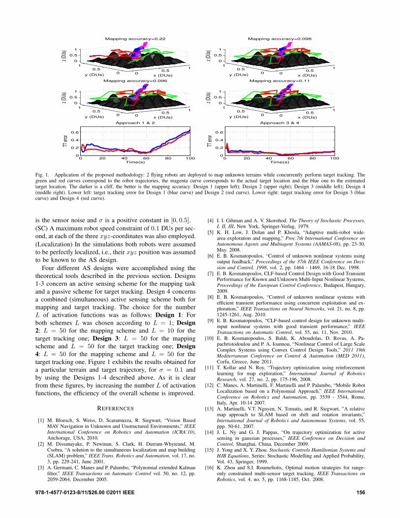
Fig. 1. Application of the proposed methodology: 2 flying robots are deployed to map unknown terrains while concurrently perform target tracking. Thegreen and red curves correspond to the robot trajectories, the magenta curve corresponds to the actual target location and the blue one to the estimatedtarget location. The darker is a cliff, the better is the mapping accuracy. Design 1 (upper left); Design 2 (upper right); Design 3 (middle left); Design 4(middle right). Lower left: target tracking error for Design 1 (blue curve) and Design 2 (red curve). Lower right: target tracking error for Design 3 (bluecurve) and Design 4 (red curve).

is the sensor noise and σ is a positive constant in [0, 0.5].

(SC) A maximum robot speed constraint of 0.1 DUs per sec-

ond, at each of the three xyz-coordinates was also employed.

(Localization) In the simulations both robots were assumed

to be perfectly localized, i.e., their xyz position was assumed

to be known to the AS design.

Four different AS designs were accomplished using the

theoretical tools described in the previous section. Designs

1-3 concern an active sensing scheme for the mapping task

and a passive scheme for target tracking. Design 4 concerns

a combined (simultaneous) active sensing scheme both for

mapping and target tracking. The choice for the number

L of activation functions was as follows: Design 1: For

both schemes L was chosen according to L = 1; Design

2: L = 50 for the mapping scheme and L = 10 for the

target tracking one; Design 3: L = 50 for the mapping

scheme and L = 50 for the target tracking one; Design

4: L = 50 for the mapping scheme and L = 50 for the

target tracking one. Figure 1 exhibits the results obtained for

a particular terrain and target trajectory, for σ = 0.1 and

by using the Designs 1-4 described above. As it is clear

from these figures, by increasing the number L of activation

functions, the efficiency of the overall scheme is improved.

REFERENCES

[1] M. Bloesch, S. Weiss, D. Scaramuzza, R. Siegwart, “Vision BasedMAV Navigation in Unknown and Unstructured Environments,” IEEEInternational Conference on Robotics and Automation (ICRA’10),Anchorage, USA, 2010.

[2] M. Dissanayake, P. Newman, S. Clark, H. Durrant-Whyteand, M.Csobra, “A solution to the simultaneous localization and map building(SLAM) problem,” IEEE Trans. Robotics and Automation, vol. 17, no.3, pp. 229-241, June 2001.

[3] A. Germani, C. Manes and P. Palumbo, “Polynomial extended Kalmanfilter,” IEEE Transactions on Automatic Control vol. 50, no. 12, pp.2059-2064, December 2005.

[4] I. I. Gihman and A. V. Skorohod. The Theory of Stochastic Processes,I, II, III, New York, Springer-Verlag, 1979.

[5] K. H. Low, J. Dolan and P. Khosla, “Adaptive multi-robot wide-area exploration and mapping,” Proc.7th International Conference onAutonomous Agents and Multiagent Systems (AAMAS-08), pp. 23-30,May. 2008.

[6] E. B. Kosmatopoulos, “Control of unknown nonlinear systems usingoutput feedback,” Proceedings of the 37th IEEE Conference on Deci-

sion and Control, 1998, vol. 2, pp. 1464 - 1469, 16-18 Dec. 1998.

[7] E. B. Kosmatopoulos, CLF-based Control Design with Good TransientPerformance for Known and Unknown Multi-Input Nonlinear Systems,Proceedings of the European Control Conference, Budapest, Hungary,2009.

[8] E. B. Kosmatopoulos, “Control of unknown nonlinear systems withefficient transient performance using concurrent exploitation and ex-ploration,” IEEE Transactions on Neural Networks, vol. 21, no. 8, pp.1245-1261, Aug. 2010.

[9] E. B. Kosmatopoulos, “CLF-based control design for unknown multi-input nonlinear systems with good transient performance,” IEEETransactions on Automatic Control, vol. 55, no. 11, Nov. 2010.

[10] E. B. Kosmatopoulos, S. Baldi, K. Aboudolas, D. Rovas, A. Pa-pachristodoulou and P. A. Ioannou, “Nonlinear Control of Large ScaleComplex Systems using Convex Control Design Tools,” 2011 19th

Mediterranean Conference on Control & Automation (MED 2011),Corfu, Greece, June 2011.

[11] T. Kollar and N. Roy, “Trajectory optimization using reinforcementlearning for map exploration,” International Journal of Robotics

Research, vol. 27, no. 2, pp. 175-196, 2008.[12] C. Manes, A. Martinelli, F. Martinelli and P. Palumbo, “Mobile Robot

Localization based on a Polynomial Approach,” IEEE International

Conference on Robotics and Automation, pp. 3539 - 3544, Rome,Italy, Apr. 10-14 2007.

[13] A. Martinelli, V.T. Nguyen, N. Tomatis, and R. Siegwart, ”A relativemap approach to SLAM based on shift and rotation invariants,”International Journal of Robotics and Autonomous Systems, vol. 55,ppp. 50-61, 2007.

[14] J. L. Ny and G. J. Pappas, “On trajectory optimization for activesensing in gaussian processes,” IEEE Conference on Decision and

Control, Shanghai, China, December 2009.[15] J. Yong and X. Y. Zhou. Stochastic Controls Hamiltonian Systems and

HJB Equations, Series: Stochastic Modelling and Applied Probability,Vol. 43, Springer, 1999.

[16] K. Zhou and S.I. Roumeliotis, Optimal motion strategies for range-only constrained multi-sensor target tracking, IEEE Transactions on

Robotics, vol. 4, no. 5, pp. 1168-1185, Oct. 2008.

978-1-4577-0123-8/11/$26.00 ©2011 IEEE 156


Recommended