A Game-Theoretic Study on Non-MonetaryIncentives in Data Analytics Projects with Privacy

ImplicationsMichela Chessa

EURECOMSophia Antipolis, France

michela.chessa@eurecom.fr

Jens GrossklagsThe Pennsylvania State University

University Park, PA, USAjensg@ist.psu.edu

Patrick LoiseauEURECOM

Sophia Antipolis, Francepatrick.loiseau@eurecom.fr

Abstract—The amount of personal information contributed byindividuals to digital repositories such as social network siteshas grown substantially. The existence of this data offers un-precedented opportunities for data analytics research in variousdomains of societal importance including medicine and publicpolicy. The results of these analyses can be considered a publicgood which benefits data contributors as well as individuals whoare not making their data available. At the same time, the releaseof personal information carries perceived and actual privacy risksto the contributors. Our research addresses this problem area.

In our work, we study a game-theoretic model in whichindividuals take control over participation in data analyticsprojects in two ways: 1) individuals can contribute data ata self-chosen level of precision, and 2) individuals can decidewhether they want to contribute at all (or not). From the analyst’sperspective, we investigate to which degree the research analysthas flexibility to set requirements for data precision, so thatindividuals are still willing to contribute to the project, and thequality of the estimation improves.

We study this tradeoff scenario for populations of homo-geneous and heterogeneous individuals, and determine Nashequilibria that reflect the optimal level of participation andprecision of contributions. We further prove that the analyst cansubstantially increase the accuracy of the analysis by imposing alower bound on the precision of the data that users can reveal.

Index Terms—Non-cooperative game, public good, privacy,population estimate, data analytics, non-monetary incentives

I. INTRODUCTION

A. Background

The seminal “How much Information Project?” report pub-lished in 2000 concluded that between 1 and 2 exabytes ofunique information were produced worldwide per year whichtranslated into about 250 megabytes of information for everyhuman being [1], [2]. While those figures were (and are still)largely driven by commercial production of information, inrecent years the amount of personal information producedby individuals has grown substantially. Now, Facebook aloneabsorbs about 220 petabytes of user-contributed data each year[3]. Recognizing the opportunities to economically benefitfrom this growth, personal data has been heralded as the“New Oil” of the 21st Century [4]. Similarly, opportunities areincreasingly taken advantage of to utilize the data for research.

From the individual’s perspective the latter trend results in atradeoff calculus.

On the one hand, individuals recognize that many complexchallenges with societal importance, such as public healthconsiderations, market-research or political decision-making[5], may benefit from a more rigorous analytic treatment,thanks to data analytics research and the newly-won abundanceof personal information. From this perspective, many analyticresults that are based on individuals’ personal data can beinterpreted as public goods with societal importance. Forexample, advancements to better understand certain illnessesdo not only potentially benefit the contributors of personaldata, but are often made accessible to people in a particulardomain (e.g., citizen of a country, individuals in a certainsocial status or demographic category, or everybody).

On the other hand, the same individuals have justifiedprivacy concerns about the release of their personal data. Thereasons for privacy concerns can be quite diverse as outlinedin Solove’s privacy taxonomy [6]. Individuals may perceivethe release and use of their data as an intrusion of theirpersonal sphere [7], [8], or as a violation of their dignity [9]. Inaddition, they may fear this data can be abused for unsolicitedadvertisements, or social and economic discrimination (e.g.,[10], [11]).

The published studies demonstrate the need to organize thecollection of personal data when facing this users’ tradeoffscenario, by implementing effective control and participationmechanisms. It has been shown that a majority of individualsconsider it as important to be able to exercise control overthe release of their personal data [12]. For example, a numberof empirical studies have provided evidence for such desiresfor control in the medical domain [13]–[15]. Moreover, evenif data privacy provisions are met, many respondents wouldstill require notice and consent over their medical data release[14]–[16]. Finally, several studies show a high overall concernfor certain data releases. For example, a meta-review ofpublished surveys showed that in some contexts a majority ofrespondents were entirely uncomfortable with health researchif effective notice and consent practices were absent [17].Similar findings can be shown for other problem domains.

arX

iv:1

505.

0241

4v1

[cs

.GT

] 1

0 M

ay 2

015

B. Problem Statement and Approach

Our research addresses the problem area identified in theabove section. In this paper, we propose individuals’ incentivesto participate in data analysis projects. These individuals face atradeoff between having privacy cost associated with their datarelease, but also deriving benefits from the analysis’ results.

We are particularly motivated by the scenario when dataabout individuals is already stored in a secure database for adifferent primary purpose (e.g., social networking or medicalservices). An analyst can then request the participation ofindividuals in a data analysis project (via a notice and consentprocess with negligible cost) that provides a public good. Moreprecisely, individuals make decisions about the release of aprivate value given a population-relevant metric. The analysthas the objective of accurately estimating the associated pop-ulation average for all individuals.

Our main focus is on understanding the incentives ofindividuals to participate, and of the analyst to shape thisdecision-making process. From each individual’s perspective,control over participation takes two forms: 1) individuals cancontribute data at a self-chosen level of precision, and 2)individuals can decide whether they want to contribute atall (or not). From the analyst’s perspective, we investigateto which degree the research analyst has flexibility to setrequirements for data precision, so that individuals are stillwilling to contribute to the project, and the quality of theestimation improves.

Our work assumes that incentives for participation are non-monetary; that is, the main driver for data contributions is theinterest in the derived public good. We base this assumptionon the observation that direct monetary compensation forpersonal information has so-far received very little tractionin the market for personal information, and that it meets littleacceptance in consumer surveys.1

We follow a game-theoretic approach to investigate theoutlined trade-off calculus. We iteratively develop a model,where the starting point is a simplified version of the workby [18], that captures the interaction between an analyst anda set of individuals who have control over the release ofinformation to the analyst. We conduct a rigorous analysis andderive concrete results about the precision of contributions, thequality of the population estimate, and the overall willingnessto contribute to the project.

C. Contributions

In this paper, we consider critical facets of realistic pri-vacy decision-making, striking a good balance between modelcomplexity and potential impact. We rigorously analyze ageneral model where users optimize a cost composed of anindividual privacy cost and an estimation cost that captures thepublic good component of the analyst’s estimation, both givenby arbitrary functions satisfying relatively mild assumptions.

1While related empirical data is sparse, a survey reported that only about25% of the surveyed population would accept monetary compensation for per-sonal information [12]. In contrast, offering discounts or free products/servicesfor personal information is a common practice.

In particular, we consider a general case with a continuousprivacy cost function which allows users to choose a privacylevel in a continuum of choices (and not simply a 0-1 choice).We first analyze the homogeneous agents case, and thenwe extend our results to the case of heterogeneous agents,providing in detail the actions the analyst should take in orderto improve the estimation. Evidence that privacy concernsare heterogeneous is a particularly central cornerstone of theprivacy literature [19], and such an extension is fundamentalfor the applicability of the model.

For both the homogeneous and the heterogeneous case, wedetermine Nash equilibria indicating the number of contrib-utors and the optimal contribution levels by the individuals.We further prove that the analyst can increase the populationestimate’s accuracy simply by imposing a lower bound on theprecision of the data that users can reveal (i.e., by restrictingthe level of precision of data contributions). While, for a fixedpopulation of users providing data, increasing the precisionof each data point clearly improves the population estimate’sprecision, the surprising and important aspect of our result liesin that the scheme remains incentive compatible, i.e., usersare still willing to provide data with a higher precision ratherthan dropping out. We also show how to tune the minimumprecision level the analyst should set in order to optimize thepopulation estimate’s accuracy. In our numerical simulations,we find a maximum improvement of the population estimate’saccuracy in the order of 20− 40%.

We further provide extensions of our modeling framework.First, we discuss a two-stage game in which the analystmay first recruit participants that commit to provide privatedata with a minimum precision; and only in a second stage,these agents would be asked to disclose their information.This captures scenarios in which agents are recruited forspecific studies. Second, we also address the issue of costlyacquisition of agents and their data for analysis purposes.While the no-cost-per-agent assumption we make throughoutthe remainder of the paper is a standard approach in most ofthe literature on public goods, we believe that certain practicalscenarios require the appreciation of cost considerations, andthis extension further completes our framework.

Our results provide a widely applicable method to increasethe provision of a public good above voluntary contributions,simply by restricting the agents’ strategy spaces. This methodis attractive by its simplicity compared for instance to otherschemes that involve monetary transfers; and could find uti-lization in other public good contexts.

Understanding the trade-off between privacy, the qualityof data analysis results, and willingness-to-participate in suchprojects is of current and growing importance. Analysts shouldnot rely on overly broad or ineffective (take-it-or-leave-it)notice and consent procedures that do not accurately reflectindividuals’ preferences. In many privacy-sensitive scenariossuch as involving medical data it is particularly unethical todeprive individuals of their opportunities to make decisionsabout their data, and whether they want to be involved incertain analysis projects. However, better insights about the

involved incentive structures are needed to guide public policyand advancements of privacy-aware data analysis.

Preliminary versions of some of the results presented inthis paper appeared in our short paper [20], in the context of asimplified model with monomial privacy cost, linear estimationcost and homogeneous agents. Here, we provide results forthe general framework introduced above that relaxes such as-sumptions, we provide detailed results of practical importanceon how the analyst should optimally selected the minimumprecision level, and we provide several further extensions. InSection IV-C, we also provide more detailed results in thesimplified setting of [20], to qualitatively illustrate the resultsof the present paper.

D. Roadmap

Our paper is structured as follows. In Section II, wereview related work. We develop and describe our model inSection III. We conduct our analysis in detail in Section IV ona canonical case of homogeneous agents. We extend the resultsto heterogeneous agents in Section V. We discuss extensionsto our model in Section VI, and conclude in Section VII. Allproofs are relegated to the Appendix.

II. RELATED WORK

Our model draws on different lines of research includingwork on privacy in the context of data analytics, and gametheoretic and public goods models. We also briefly reviewtechnical and cryptographic approaches, and behavioral re-search on control and data sharing.

Research on the optimal design of experiments assumesthat already the stage of data collection can be influencedby the analyst in order to improve the learning of a linearmodel [21], [22]. In this paper, we allow the analyst to requiredata contributions at a certain level of precision to improvethe computation of a population estimate, which is a relatedconcept. Optimal design of experiments has been studiedfrom the perspective of incentives [23], or with the scope ofobtaining an unbiased estimator [24]. We propose to improvethe design of experiments focusing on the privacy concerns ofthe agents.

Privacy-preserving techniques in the context of data ana-lytics have a long history. Some recent papers propose newapproaches, which allow users to protect their privacy sellingaggregates of their data [25], [26]. The more classical frame-work of ε-differential privacy [27], [28], assumes that data areperturbed after an analysis has been conducted on unmodifiedinputs. That is, the analyst is considered trustworthy. In thisframework, researchers have also studied the role of incentives[29]–[32]. Our work differs, as we assume agents to be re-leasing their data independently, and an untrusted data analystwhich motivates perturbations of data before submission. Theidea of affecting the level of precision of released personaldata, adding noise in advance of data analysis has been studiedin the context of privacy-preserving data-mining (see, e.g.,[33], [34]) and specific application scenarios such as buildingdecision trees [35], clustering [36], and association rule mining

[37]. More recently, bounds have been derived on genericinformation-theoretic quantities and statistical estimation ratesunder a local privacy model which preserves the privacy ofagents even from the learner (similarly to adding noise beforerevealing data) [38].

Recent work has also studied the combinatorial optimiza-tion problem when an analyst may buy unbiased samplesof data from different providers with given but potentiallyheterogeneous variance-price combinations [39]. In anotherrecent working paper, analysts can access unbiased samplesof private data by compensating data subjects for their datarelease according to their preferences [40]. Those studies arecomplementary to our work in which data subjects individuallydecide in a game-theoretic framework on the degree of dataaccuracy given a trade-off between their privacy and thedetermination of a socially valuable population estimate.

From a mechanism design perspective, scenarios have beenstudied where survey subjects are assumed to potentiallymisreport their private values [41], [42], however, these be-haviors are not studied in the context of a non-cooperativescenario. A mechanism design perspective is taken in [43]where the authors introduce monetary payments to createincentives for agents to give high quality data. Here, wedo not consider monetary payments. A strategic approach isfollowed in [18], where an analyst performs a linear regressionbased on users’ perturbed data. The authors in [18] treat theestimation accuracy as a public good and study the equilibriumaccuracy achieved without introducing monetary payments andthe resulting price of anarchy. Our starting point is a simplifiedversion of the model in [18]. We continue this line of researchby studying the benefits of restricting potential perturbationon the population estimate accuracy, and the incentives forparticipation in a game-theoretic framework.

Our research is also relevant to the context of the provi-sioning of public goods [44]. Our results show a new way ofincreasing the public good provision by restricting the agents’possible actions, as opposed to using monetary incentives. Inaddition, studies on interdependent privacy which capture theidea that data sharing by one agent impacts the privacy of otherconnected agents is complementary to our work [45], [46].We model the scenario when sharing creates privacy risks forindividuals, but positive benefits for all agents.

The aforementioned theoretical works are complemented bytechnical approaches (which do not utilize insights from game-theory) such as secure hardware-based private informationretrieval which can be applied, for example, in the contextof online behavioral advertisement [47]; see also other ap-proaches for privacy-preserving online targeted advertisements[48]. Similarly, multi-party secure computation has been usedto facilitate the fitting of logistic regression when data areheld by separate parties [49], and homomorphic encryption hasbeen applied to the scenario of linear regression [50]. Secure-computation notions of privacy have also been used in com-bination with game theory for privacy-preserving mechanismdesign [51], [52].

To facilitate the privacy negotiation process between a data

subject and an analyst, different technical protocols have beenproposed. Several works are connected to the Platform for Pri-vacy Preferences Project (P3P) which offers a protocol allow-ing data collectors (e.g., websites) to declare their intended useof information they collect about data subjects [53], and alsoprovides agent tools for the user to manage those data requests[54], [55]. More recent work, for example, addresses specificproblem areas such as personalization [56]. Those mechanismsallow for user-specified policies regarding participation, butalso minimum requirements for (not necessarily truthful) datasharing as specified by the analyst.

Research on user preferences and behaviors with respect toprivacy has produced several results relevant to the context ofour work. A survey study has shown that over 90% of therespondents agreed with the definition of privacy as controlof personal information [12] which presumably would includean interest to decide over the participation in data analysisprojects. In hypothetical scenarios, individuals typically reporthigh attitudinal valuations for their private data [57]. However,in experiments with actual private data transfers researchershave observed low thresholds for the release of such data inexchange for free services/goods or discounts [19], [58], [59].A root cause for this privacy dichotomy is the complexityof understanding personal information exchanges and theirconsequences [12].

The intricacies of human decision making have also beenstudied specifically focusing on the notion of control overinformation exchanges. Laboratory and online experimentshave shown that control options have to be added with careto practically relevant scenarios [60]–[62]. For example, suchoptions can elevate individuals’ propensity to engage in riskierdisclosures because their mere presence can contribute to alowering of concerns over privacy [60]. Another experimentalstudy found that allowing individuals to customize personaldata exchanges does not increase the number of transactionseven though individuals were able to exclude unwanted aspectsof those transactions [63]. Overall the understanding of the in-volved attitudes and behaviors is still work in progress. In ourpaper, we propose a process that is relatively straightforwardto implement and to understand from a user perspective. How-ever, approaches that fully accommodate the stated behavioralhurdles remain the subject of future work for behavioral aswell as theoretical scientists.

III. THE MODEL

In this section, we present our model in detail. We describethe strategic interaction between the individuals (which wealso refer to as agents), whose information is contained ina data repository, and how the analyst, wishing to observethe data and to perform a statistical analysis, may modify theestimation by varying selected parameters. The linear modelapproach we take here builds on the work of [18].

A. The Data Repository of Personal Data

Let N = {1, . . . , n} denote the set of agents, whosepersonal data are contained in the data repository. In particular,

we suppose that each agent i ∈ N is associated with aprivate variable yi ∈ R, which contains sensitive information.Throughout our analysis, we suppose that there exists yM ∈ R,s.t., the private variables are of the form

yi = yM + εi, ∀i ∈ N, (1)

where εi are i.i.d., zero-mean random variables with finitevariance σ2 < ∞, which capture the inherent noise. Westress that we make no further assumptions on the noise; inparticular, we do not assume it is Gaussian. As a result, ourmodel applies to a wide range of statistical inference problems,even cases where the distribution of variables is not known.

Paramter yM represents the mean of the private variablesyi, and its knowledge is valuable to the analyst, for exampleas it allows him to predict the private variable of any agentwhose data cannot be known (because it is not contained in therepository at that given moment, kept private by its owner, isnot accessible due to limited computing resources, etc.). Theanalyst wishes to observe the available private variables yi andto compute their average as an estimation of yM . In our model,we suppose that the analyst does not know the mean yM , thathe wishes to estimate, but he knows the variance σ2. We arguethat observing the variability of an attribute in a population iseasier than estimating the mean, both for the analyst and forthe population (in [64], for example, the authors show howindividuals value their age and weight information accordingto the relative variability).

B. The Precision and the Analyst’s Estimation

We suppose that the analyst cannot directly access theprivate variables, rather she needs to ask the agents for theirconsent to be able to retrieve the information. As such, theagents have full control over their own private variables, andthey have the choice to authorize or to deny the analyst’srequest. In particular, if wishing to contribute, but concernedabout privacy, an agent can authorize the access to a perturbedvalue of the private variable. The perturbed variable hasthe form yi = yi + zi, where zi is a zero-mean randomvariable with variance σ2

i . We assume that the {zi}i∈N areindependent and are also independent of the inherent noisevariables {εi}i∈N . In practice, the agent chooses a givenprecision λi which corresponds to the inverse of the aggregatevariance (inherent noise, plus artificially added noise) of theperturbed variable yi, i.e.,

λi = 1/(σ2 + σ2i ) ∈ [0, 1/σ2], ∀i ∈ N.

In the choice of the precision level, we have the following twoextreme cases:(i) when λi = 0, agent i has very high privacy concerns.

This corresponds to adding noise of infinite variance or,equivalently, this represents the fact that agent i deniesthe access to her data;

(ii) when λi = 1/σ2, agent i has very low privacy concerns.This corresponds to authorizing the access to the realprivate variable yi, without adding any additional noiseto the data.

The strategy set [0, 1/σ2] contains all the possible choicesfor agent i: denying, authorizing, or any intermediate level ofprecision (which captures a wide range of privacy concernsas documented in behavioral studies [19]). We denote by λ =[λi]i∈N the vector of the precisions.

Once each agent i ∈ N has made her choice about thelevel of precision λi and, consequently, the perturbed variableyi has been computed, the analyst has access to both the set ofprecisions and the set of perturbed variables. Then, the analystestimates the mean as

yM (λ) =

∑i∈N λiyi∑i∈N λi

, (2)

where perturbed variables with higher precision (i.e., smallervariance) receive a larger weight. This estimator is the standardgeneralized least squares estimator. It minimizes a weightedsquare error in which the i-th term is weighted by the precisionof the perturbed variable yi. This estimator is unbiased, i.e.,E[yM ] = yM , and has variance

σ2M (λ) = E[(yM (λ)− yM )2] =

1∑i∈N λi

∈ [σ2/n,+∞].

(3)

In our model, the analyst aims at estimating the mean yM ,e.g., to be able to predict some additional private variables.Then, it is reasonable to assume that the analyst would use thisestimator, as it is “good” for several reasons. In particular, itcoincides with the maximum-likelihood estimator for Gaussiannoise and, most importantly, it has minimal variance amongstthe linear unbiased estimators for arbitrary noise distributions.

In the estimation, we have the following two extreme cases:(i) when λi = 0 for each i ∈ N , the variance (3) is infinite.

This corresponds to the situation in which each agentdenies the access to her data, and then the analyst cannotestimate yM ;

(ii) when λi = 1/σ2 for each i ∈ N , the analyst estimatesyM with variance σ2/n, resulting only from the inherentnoise. This corresponds to the situation in which eachagent is authorizing the access to her data with maximumprecision, i.e., no agent is perturbing her private variable.

For any level of precision in [0, 1/σ2]n, the estimated variancewill be in [σ2/n,+∞]. The set of precision vectors for whichthe estimator has a finite variance is [0, 1/σ2]n \ {(0, . . . , 0)}.

C. The Estimation Game Γ

We next describe the interaction between the agents thatresults in their choices of precisions. We assume that eachagent i ∈ N wishes to minimize a cost function Ji :[0, 1/σ2]n → R+, s.t., for each λ ∈ [0, 1/σ2]n,

Ji(λ,λ−i) = ci(λi) + f(λ), (4)

where we use the standard notation λ−i to denote the col-lection of actions of all agents but i. The cost function Ji ofagent i ∈ N comprises two non-negative components. Thefirst component ci : [0, 1/σ2] → R+ represents the privacyattitude of agent i, and we refer to it as the privacy cost:

it is the (perceived or actual) cost that the individual incurson account of the privacy violation sustained by revealing theprivate variable perturbed with a given precision. The secondcomponent f : [0, 1/σ2]n → R+ is the estimation cost, andwe assume that it takes the form f(λ) = F (σ2

M (λ)) whereF : [σ2/n,+∞) → R+ if the variance is finite, and +∞otherwise. It represents how well the analyst can estimate themean yM and it captures the idea that it is not only in theinterest of the analyst, but also of the agents, that the analystcan determine an accurate estimate of the population averageyM .

In our model, the accuracy of the estimate can be understoodas a public good, to which each user contributes with herchoice of precision λi, at a given privacy cost. From thisperspective, the assumption that the estimation cost is the samefor all agents mirrors the usual standard assumption in thepublic good literature. Throughout our analysis, we make twoadditional assumptions:

Assumption 1: The privacy costs ci : [0, 1/σ2] → R+, i ∈N , are twice continuously differentiable, non-negative, non-decreasing, strictly convex and s.t. ci(0) = c′i(0) = 0.

Assumption 2: Function F : [σ2/n,+∞) → R+ is twicecontinuously differentiable, non-negative, non-decreasing andstrictly convex.

To describe the strategic interaction between the agents, wedefine the estimation game Γ =

⟨N, [0, 1/σ2]n, (Ji)i∈N

⟩with

set of agents N , strategy space [0, 1/σ2] for each agent i ∈ Nand cost function Ji given by (4).

D. The Modified Estimation Game Γ(S, η)

As we shall see (Section IV-A), game Γ has a unique Nashequilibrium for which the variance of the estimation is largerthan the optimal one (σ2/n) due to the excess noise addedby agents to protect their privacy. We further investigate thesituation in which the analyst can modify the game and tryto mitigate the effect of agents’ privacy concerns in order toreduce the estimation cost (i.e., to improve the accuracy of theestimation obtained). Specifically, the analyst can implementthe following two variations of the model. First, she can choosea minimum precision level η ∈ [0, 1/σ2], which is equivalentto fixing a maximum variance for the noise that agents canadd to perturb their data. As it is not practically possible toforce agents to authorize the access to their data with a givenprecision, we still assume that the agents can choose to denythe authorization, which is equivalent to selecting a precisionlevel equal to zero. Second, the analyst can request the accessto the personal data to only a subset S ⊆ N of agents, withs = |S| (for example, excluding those agents who are the mostconcerned about privacy).

In the modified game, the agents are informed of the subsetof individuals who are asked to reveal their personal data,and of the minimum precision level η. They choose theirprecision λi in the range imposed by the analyst [η, 1/σ2]or decide to deny the access, i.e., select their precisionequal to 0. To analyze the strategic interaction between theagents in this variation, we define the game Γ(S, η) =

⟨S,[{0} ∪ [η, 1/σ2]

]s, (Ji)i∈S

⟩(where the cost function Ji

is still given by (4)), which is identical to Γ, except for therestricted set of agents and the restricted strategy space.

Observe that the original game Γ is a special case of thismodified game Γ(S, η), when S = N and η = 0. We analyzethe games Γ and Γ(S, η) as complete information gamesbetween the agents, i.e., we assume that the set of agents,the action sets (in particular, when present, the value of theparameter η) and the costs are known by all the agents.

IV. THE HOMOGENEOUS AGENT CASE

In this section, we detail the analysis in the symmetric casewhere all the agents have identical privacy concerns, i.e., weassume that the privacy cost functions of all agents are thesame: ci(·) = c(·) for each i ∈ N . This special case highlightsthe key aspects of our approach and provides some interestingpreliminary results that yield intuitive interpretations. We willgeneralize our results to the heterogeneous case in Section V.

A. The Estimation Game in the Homogeneous Case

We first analyze the estimation game Γ, in which all theagents in N are playing and the analyst allows them tochoose any precision level between 0 and 1/σ2. A Nashequilibrium (in pure strategy) of this game is a strategy profileλ∗ ∈ [0, 1/σ2]n satisfying

λ∗i ∈ arg minλi∈[0,1/σ2]

Ji(λi,λ∗−i), ∀i ∈ N. (5)

The game Γ with strategy space [0, 1/σ2] is a special caseof the game in [18], where the existence of a unique Nashequilibrium is established. However, our specific assumptionsallow us to characterize the equilibrium in more detail:

Theorem 1: The game Γ has a unique Nash equilibrium λ∗

s.t. λ∗i = λ∗ > 0 for each i ∈ N .The proof of this result exploits the fact that game Γ

is a potential game to characterize the Nash equilibrium.Interestingly, we observe that non-participation by everybody,i.e., λ = (0, . . . , 0), cannot be an equilibrium. Indeed, as theestimation cost diverges at λ = (0, . . . , 0), every agent hasa profitable deviation from this point since contributing anypositive λi brings the estimation cost down to a finite cost.Note, however, that this is not an artifact of the model, as itremains true if we assume that the estimation cost is boundedbut large enough to exceed the privacy cost.

We observe that, as a consequence of the symmetry ofthe game in the homogeneous case, all the agents at equi-librium choose the same precision level, which is a functionλ∗ = λ∗(n) of the total number of agents n. Then, from thediscussion above, it is clear that λ∗ cannot be zero, so that allagents contribute a positive precision.

Due to the arbitrariness of the functions F (·) and c(·), theunique Nash equilibrium cannot be written in closed form.However, it is easily computable in practice either as theminimum of the potential function (which is convex) or asthe unique solution of the following fixed point problem:

λ = g(n, λ),

where function g : N∗ × [0, 1/σ2] → [0,+∞] is defined foreach λ ∈ (0, 1/σ2] and for each n ∈ N∗ as

g(n, λ) = min

{√F ′(

1

nλ

)1

n2c′(λ), 1/σ2

}and is defined by continuity as limλ→0+ g(n, λ) for λ = 0 andfor each n ∈ N∗.

Given the unique Nash equilibrium λ∗(n), the variance (inEquation (3)) of the estimate of yM obtained by the analyst atequilibrium is also a function of n, and given by the followingexpression:

σ2M (λ∗(n)) =

1

nλ∗(n). (6)

In Propositions 1 and 2 below, we derive the properties of theequilibrium precision and of the corresponding variance, whenthe number of agents varies.

Proposition 1: The equilibrium precision level λ∗(n) satis-fies:(i) λ∗(n) is a non-increasing function of the number n of

agents, and(ii) limn→+∞ λ∗(n) = 0.

Proposition 1 states that the equilibrium contribution of eachagent decreases as the number of agents increases (Part (i)).This is a standard property in public good problems as agentschoose their equilibrium contribution such that the marginalincrease in the contribution cost equates the marginal decreasein the estimation cost, and the marginal effect of a single agentdecreases when the number of agent increases. Proposition 1-(ii) shows that, in the limit when n becomes very large, thecontribution of each agents tends to zero (i.e., each agent addsa variance tending to infinity to her data). It is interesting tonotice that, given that the equilibrium prevision level λ∗(n)goes to zero as n goes to infinity, the variance (6) cannotdecrease in 1/n as in the standard case of the empirical meanof iid random variables of equal variance. This is because,here, the variance of each data point (or random variable)increases as the number of points increases. Yet, as the nextproposition shows, the variance of the mean’s estimate is stillnon-increasing.

Proposition 2: The equilibrium variance of the estimate ofyM satisfies:(i) σ2

M (λ∗(n)) is a non-increasing function of the numberof agents n, and

(ii) limn→+∞ σ2M (λ∗(n)) = 0.

Proposition 2-(i) shows that, for the analyst, it is alwaysbetter to have a larger number of agents giving data despitethe fact that, when the number of agents increases, eachagent gives data with smaller precision (see Proposition 1).Proposition 2-(ii) analyzes the case of a large number of agentsn. Interestingly, when n gets large, the variance goes to zero,though at a rate smaller than 1/n as mentioned above. (Wegive an expression of the rate in Section IV-C for specialfunctions F and c).

B. The Modified Estimation in the Homogeneous Case

We now move to the case where the analyst can restrictthe set of agents, thereby asking to access the data of onlya subgroup of them, and potentially introducing a minimumprecision level η ∈ [0, 1/σ2]. The final goal is to improvethe estimation accuracy; formally, to estimate the mean yMwith a variance strictly smaller than σ2

M (λ∗(n)). We assumethat the set S ⊆ N of agents who can authorize access totheir data (i.e., who are solicited by the analyst) is fixed, andwe analyze how the estimation varies while moving only theparameter η. This variant is modeled by the game Γ(S, η)defined in Section III-D, where η is now the only variable ofthe model. We suppose that the equilibrium precision level forthe game Γ(S, 0) is s.t. λ∗(s) 6= 1/σ2 since, otherwise, theestimation would already be optimal with variance σ2/s forη = 0.

A Nash equilibrium (in pure strategy) of the game Γ(S, η)is a strategy profile λ∗ ∈

[{0} ∪ [η, 1/σ2]

]ssatisfying

λ∗i ∈ arg minλi∈{0}∪[η,1/σ2]

Ji(λi,λ∗−i), ∀i ∈ S. (7)

In the following theorem, we show that, if the analyst choosesa minimum precision level that is not “too big”, the agents arestill wishing to authorize access to their data at equilibrium.Recall that S ⊆ N denotes the set of agents solicited by theanalyst (who are the players of the game Γ(S, η)) and thats = |S| denotes its cardinal.

Theorem 2: If s = 1, then for any η ∈ [0, 1/σ2], Γ(S, η)has a unique Nash equilibrium λ∗(s, η) = max {λ∗(1), η}.If s > 1, then there exists a unique parameter η∗(s) ∈[0, 1/σ2] s.t.:(i) for any η ∈ [0, η∗(s)], Γ(S, η) has a unique Nash

equilibrium λ∗(s, η), s.t., λ∗i (s, η) = λ∗(s, η) for eachi ∈ S, with

λ∗(s, η) =

{λ∗(s) if 0 ≤ η ≤ λ∗(s)η if λ∗(s) < η ≤ η∗(s);

(8)

(ii) for any η ∈ (η∗(s), 1/σ2], there does not exist a Nashequilibrium λ∗(s, η) s.t. λ∗i (s, η) 6= 0 for each i ∈ S.

Theorem 2 introduces the quantity η∗(s) which, as we willsee, is crucial for the analyst. Similarly to λ∗(s), the value ofη∗(s) cannot be written in closed form, but it can be computedas the unique solution of the following fixed point problem:

η = g(s, η),

where function g : N∗ × [0, 1/σ2] → [0,+∞] is defined foreach η ∈ (0, 1/σ2] and for each n ∈ N∗ as

g(s, η) = min

F(

1(s−1)η

)− F

(1sη

)c(η)

· η, 1/σ2

and is defined by continuity as limη→0+ g(s, η) in η = 0 foreach n ∈ N∗. We can also show that λ∗(s) < η∗(s) for all s(we obtain this result inside the proof of Theorem 3).

Theorem 2 characterizes the Nash equilibrium for differentvalues of the parameter η. We observe that, as a consequenceof the symmetry of the game, when η ∈ [0, η∗(s)], the uniqueequilibrium of Γ(S, η) is still symmetric, as it was for theunique equilibrium of the original game Γ. More specifically,if the analyst sets a minimum precision level η smaller thanthe unique equilibrium precision level λ∗(s) of game Γ, therestriction of the strategy set does not have any effect on theoutcome of the game. On the other hand, if the analyst setsa minimum precision level η in the interval (λ∗(s), η∗(s)],all agents are still willing to participate with a precision η >λ∗(s). This result matches with intuition, because even thoughagents’ marginal costs are higher than the marginal benefits(the equilibrium choice is on the border of the strategy space[η, 1/σ2]), their costs are still lower than if they choose aprecision level zero. Therefore, agents do not have incentivesto deviate. In the remaining range (η∗(s), 1/σ2], there doesnot exist an equilibrium such that each agent chooses a non-zero precision level. If there exist Nash equilibria, they aresuch that a subset S′ ⊂ S of agents choose the non-zeroprecision level λ∗(s′, η), while the others choose zero. Thepossible existence of these equilibria is not relevant for ouranalysis. In fact, such an equilibrium would provide the sameestimation that the analyst can obtain by implementing thegame Γ(S′, η) and, as we see in the following theorem, theestimation improves by maximizing the number of agents inthe game.

The previous theorem is an important stepping stone allow-ing us to establish the main result of this section:

Theorem 3: The estimation variance at equilibrium is min-imal for S = N and η = η∗(n). Moreover, we have

σ2M (λ∗(n, η∗(n))) < σ2

M (λ∗(n)),

that is, setting a minimum precision level η = η∗(n) strictlyimproves the estimation.Theorem 3 shows that the analyst can indeed improve thequality of the estimation by setting a minimum precisionlevel. It establishes that it is optimal, for the analyst, tosolicit access to the private variable of all the agents whosedata is contained in the data repository; and it provides theoptimal minimum precision level η = η∗(n) that the analystshould set to maximize the estimation precision. (Recall thatη∗(n) can be easily computed from the model’s parameters bysolving a fixed point problem.) Overall, Theorem 3 providesan implementable mechanism through which the analyst canimprove the quality of the data provided by each user byimposing restrictions on the variance that users can add. Inthe next section, we study a special case with simple functionsF (·) and c(·) in order to quantify precisely the improvementachieved.

C. The Special Case with Monomial Privacy Costs and LinearEstimation Cost

In this section, we illustrate the results of the previoussections on the special case where the privacy cost is monomial

and the estimation cost is linear; i.e., we assume that the costfunction in (4) has the form

Ji(λi,λ−i) = cλki + σ2M (λ), (9)

where c ∈ (0,∞) and k ≥ 2 are constants. Note that,without loss of generality, in the linear estimation cost, weomit the constant factor (adding a constant to the cost doesnot modify the game solutions) as well as the slope factor(adding it would give an equivalent game with constant crescaled). For this special case, we can determine both theequilibrium precision (without a minimum precision level) andthe optimal minimum precision level in closed form. We canthen graphically depict how the quantities vary while movingthe model parameters, and explicitly compute the estimationimprovement. A preliminary analysis of the simplified modelwith costs as in (9) was provided in our previous work [20]; weprovide an extended analysis of this special case here thanksto the results of the previous section.

In the special case of costs given by (9), the equilibriumprecision chosen by the agents in the game Γ simplifies to:

λ∗(n) =

(

1

ckn2

) 1k+1

if(

1

ckn2

) 1k+1

≤ 1/σ2

1/σ2 if(

1

ckn2

) 1k+1

> 1/σ2.

(10)

As we have seen in the previous section (Theorem 3), it isoptimal for the analyst to request access to the data of allagents in N . In this special case, the corresponding optimalminimum precision level becomes

η∗(n) =

(

1

cn(n− 1)

) 1k+1

if(

1

cn(n− 1)

) 1k+1

≤ 1/σ2

1/σ2 if(

1

cn(n− 1)

) 1k+1

> 1/σ2.

Writing explicitly these two key quantities, we can imme-diately notice that, when c increases, i.e., when the agents aremore concerned about privacy, they choose at equilibrium asmaller precision level λ∗(n). Further, the minimum precisionlevel η∗(n) proposed by the analyst becomes smaller, if theagents are more sensitive about the protection of their data. Inthis special case, the properties of the results for the genericcase are easy to spot. For instance, we have λ∗(n) < η∗(n)for each n ∈ N∗, and both of these quantities decrease and goto zero when n increases and goes to +∞.

Most interestingly, the closed-form expressions that we havefor this special case allow us to analyze the rate of decreaseof the variance, and to quantify the improvement that can beachieved by imposing a minimum precision level. For n largeenough (such that both λ∗(n) and η∗(n) are strictly smallerthan 1/σ2), the variance at equilibrium level λ∗(n) of gameΓ is given by

σ2M (λ∗(n)) =

1

n(

1ckn2

) 1k+1

,

k1

k+

1

2 3 4 5 6 7 8 9 101.22

1.24

1.26

1.28

1.3

1.32

1.34

k

0 100 200 300 400 5001

1.05

1.1

1.15

1.2

1.25

1.3

1.35

1.4

k

Fig. 1: Asymptotic improvement of the estimation choosingthe optimum precision level η∗ for values of k = 2, . . . , 10and for values of k = 2, . . . , 500.

while the variance at equilibrium level λ∗(n, η∗(n)) of gameΓ(N, η∗(n))) where the optimal minimum precision level isset is given by

σ2M (λ∗(n, η∗(n))) =

1

n(

1cn(n−1)

) 1k+1

.

Both appear to have the same rate of decrease in n−k+1k+1 which

is smaller than n−1 but becomes closer to n−1 as k tendsto infinity. Intuitively, as the privacy cost becomes closer toa step function, the equilibrium precision level becomes lessdependent on the number of agents so that we get closer tothe case of averaging iid random variables of fixed variance.Consequently, for n large enough, the improvement is givenby a factor:

σ2M (λ∗(n))

σ2M (λ∗(n, η∗(n)))

=

(kn

n− 1

) 1k+1

> 1, (11)

which asymptotically becomes constant:

σ2M (λ∗(n))

σ2M (λ∗(n, η∗(n)))

∼n→∞ k1

k+1 . (12)

Interestingly, we notice that this ratio of variances (charac-terizing the improvement when setting the optimal minimumprecision level) depends on k, but not on c. (This holds evenbefore the asymptotic regime, as long as n is large enough suchthat both λ∗(n) and η∗(n) are strictly smaller than 1/σ2.)

Figure 1 illustrates the asymptotic improvement ratio (12)for different values of k. We observe that it is bounded, itgoes to 1 for large k’s and it is in the range of 25 − 30%improvement for values of k around 2 − 10. Given that theratio (11) converges towards its asymptote from above, thisasymptotic improvement represents a lower bound of theimprovement the analyst can achieve by implementing ourmechanism with any finite number of agents n.

V. THE HETEROGENEOUS AGENT CASE

The previous section presents an exhaustive analysis of ourmodel in the homogeneous case, i.e., when the agents exhibitthe same privacy concerns. This simplified approach enables usto derive a first set of concrete results, intuition and qualitativeunderstanding of the model and of the minimum contribution

level mechanism. The results directly apply to homogeneouspopulations, and can serve as a first approximation by theanalyst in other cases, i.e., whenever she does not have specificinformation about the agents. Indeed, the results are functionsonly of the total number of agents, and in practice this couldrepresent the only available detail about the agents whose datais stored in the data repository. However, not all populationsare homogeneous in their privacy concerns and having moredetails about the different privacy concerns of the agentsallows for a customized analysis. Measuring how individualsvalue their private information is non-trivial, but researchershave conducted direct measurement surveys [57], [65] andvarious laboratory/field experiments [58], [59] allowing for anapproximate ranking of users’ privacy concerns, and context-specific valuations.

With this scope, we now extend our approach to the casein which the analyst faces a heterogeneous population. In thissection, we remove the restricting hypothesis of homogeneityof the agents, and we allow them to exhibit different privacyconcerns. Formally, the privacy cost function of an agent i ∈N is equal to ci(·), where all the ci’s satisfy Assumption 1,but may be different from each other.

In order to model this situation, we follow the sameapproach that we used for the homogeneous case, i.e., wefirst analyze the situation in which the analyst implementsthe game Γ, without restricting the set of agents and withoutintroducing a minimum precision level. Thereafter, we showhow the analyst can improve the estimation by implementinga modified game Γ(S, η).

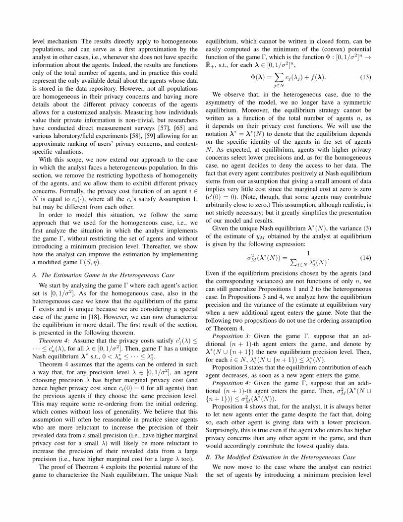
A. The Estimation Game in the Heterogeneous Case

We start by analyzing the game Γ where each agent’s actionset is [0, 1/σ2]. As for the homogeneous case, also in theheterogeneous case we know that the equilibrium of the gameΓ exists and is unique because we are considering a specialcase of the game in [18]. However, we can now characterizethe equilibrium in more detail. The first result of the section,is presented in the following theorem.

Theorem 4: Assume that the privacy costs satisfy c′1(λ) ≤· · · ≤ c′n(λ), for all λ ∈ [0, 1/σ2]. Then, game Γ has a uniqueNash equilibrium λ∗ s.t., 0 < λ∗n ≤ · · · ≤ λ∗1.

Theorem 4 assumes that the agents can be ordered in sucha way that, for any precision level λ ∈ [0, 1/σ2], an agentchoosing precision λ has higher marginal privacy cost (andhence higher privacy cost since ci(0) = 0 for all agents) thanthe previous agents if they choose the same precision level.This may require some re-ordering from the initial ordering,which comes without loss of generality. We believe that thisassumption will often be reasonable in practice since agentswho are more reluctant to increase the precision of theirrevealed data from a small precision (i.e., have higher marginalprivacy cost for a small λ) will likely be more reluctant toincrease the precision of their revealed data from a largeprecision (i.e., have higher marginal cost for a large λ too).

The proof of Theorem 4 exploits the potential nature of thegame to characterize the Nash equilibrium. The unique Nash

equilibrium, which cannot be written in closed form, can beeasily computed as the minimum of the (convex) potentialfunction of the game Γ, which is the function Φ : [0, 1/σ2]n →R+, s.t., for each λ ∈ [0, 1/σ2]n,

Φ(λ) =∑j∈N

cj(λj) + f(λ). (13)

We observe that, in the heterogeneous case, due to theasymmetry of the model, we no longer have a symmetricequilibrium. Moreover, the equilibrium strategy cannot bewritten as a function of the total number of agents n, asit depends on their privacy cost functions. We will use thenotation λ∗ = λ∗(N) to denote that the equilibrium dependson the specific identity of the agents in the set of agentsN . As expected, at equilibrium, agents with higher privacyconcerns select lower precisions and, as for the homogeneouscase, no agent decides to deny the access to her data. Thefact that every agent contributes positively at Nash equilibriumstems from our assumption that giving a small amount of dataimplies very little cost since the marginal cost at zero is zero(c′(0) = 0). (Note, though, that some agents may contributearbitrarily close to zero.) This assumption, although realistic, isnot strictly necessary; but it greatly simplifies the presentationof our model and results.

Given the unique Nash equilibrium λ∗(N), the variance (3)of the estimate of yM obtained by the analyst at equilibriumis given by the following expression:

σ2M (λ∗(N)) =

1∑j∈N λ

∗j (N)

. (14)

Even if the equilibrium precisions chosen by the agents (andthe corresponding variances) are not functions of only n, wecan still generalize Propositions 1 and 2 to the heterogeneouscase. In Propositions 3 and 4, we analyze how the equilibriumprecision and the variance of the estimate at equilibrium varywhen a new additional agent enters the game. Note that thefollowing two propositions do not use the ordering assumptionof Theorem 4.

Proposition 3: Given the game Γ, suppose that an ad-ditional (n + 1)-th agent enters the game, and denote byλ∗(N ∪ {n + 1}) the new equilibrium precision level. Then,for each i ∈ N , λ∗i (N ∪ {n+ 1}) ≤ λ∗i (N).

Proposition 3 states that the equilibrium contribution of eachagent decreases, as soon as a new agent enters the game.

Proposition 4: Given the game Γ, suppose that an addi-tional (n + 1)-th agent enters the game. Then, σ2

M (λ∗(N ∪{n+ 1})) ≤ σ2

M (λ∗(N)).Proposition 4 shows that, for the analyst, it is always better

to let new agents enter the game despite the fact that, doingso, each other agent is giving data with a lower precision.Surprisingly, this is true even if the agent who enters has higherprivacy concerns than any other agent in the game, and thenwould accordingly contribute the lowest quality data.

B. The Modified Estimation in the Heterogeneous CaseWe now move to the case where the analyst can restrict

the set of agents by introducing a minimum precision level

η ∈ [0, 1/σ2]. Again, her final goal is to improve theestimation accuracy. We consider at first the set of agentsS ⊆ N to be fixed, and we analyze how the estimation varieswhile moving only the parameter η. This variant is modeledby the game Γ(S, η) defined in Section III-D, where η isnow the only variable of the model. We denote by λ∗(S)the equilibrium precision level for the game Γ(S, 0), and wesuppose that it is such that there exists at least one agent i ∈ Ss.t. λ∗i (S) 6= 1/σ2; otherwise the estimation is already optimalwith variance σ2/s for η = 0.

The next result extends Theorem 2 to the heterogeneouscase. We show that, if the analyst selects a minimum precisionlevel which is not “too high”, at equilibrium, all the agents(even the most concerned about privacy) are still willing toauthorize access to their data (with perturbation).

Theorem 5: As in Theorem 4, assume that the privacy costssatisfy c′1(λ) ≤ · · · ≤ c′n(λ), for each λ ∈ [0, 1/σ2]. Giventhe set of agents S ⊆ N , with cardinality s ≥ 1:(i) if s = 1, then for any η ∈ [0, 1/σ2], Γ(S, η) has a unique

Nash equilibrium λ∗1(S, η) = max {λ∗1(S), η};(ii) if s > 1, then there exists a parameter η∗(S) ∈

(λ∗(S), 1/σ2] such that, for any η ∈ [0, η∗(S)], Γ(S, η)has a unique Nash equilibrium λ∗(S, η) with λ∗i (S, η) >0 for all i ∈ S.

Theorem 5 introduces a parameter η∗(S) such that if theanalyst sets a minimum precision level in [0, η∗(S)], even themost privacy-concerned of the agents in S does not have anincentive to deviate to a zero precision level. As the theoremis stated, η∗(S) is not unique (any value smaller than a validη∗(S) but still larger than λ∗(S) will be suitable). However,let η∗(S) be s.t.

cn(λ∗n(S, η∗(S))) = (15)

F

(1∑

j∈N,j 6=n λ∗j (S, η

∗(S))

)− F

(1∑

j∈N λ∗j (S, η

∗(S))

),

where λ∗(S, η∗(S)) is the local minimum of the poten-tial function Φ defined as in (13), but on the domain[η∗(S), 1/σ2]s. We can prove that this η∗(S) is unique, that itsatisfies Theorem 5-(ii) and we conjecture that this definitiongives the largest possible parameter satisfying Theorem 5-(ii).

The result of Theorem 5 allows us to establish the mainresult of this section:

Theorem 6: As in Theorem 4, assume that the privacy costssatisfy c′1(λ) ≤ · · · ≤ c′n(λ), for each λ ∈ [0, 1/σ2]. Letη∗(N) be as in Theorem 5-(ii) for S = N . The analyst can im-prove the estimation by implementing the game Γ(N, η∗(N))with minimum precision level η∗(N), i.e.,

σ2M (λ∗(N, η∗(N))) < σ2

M (λ∗(N)).

Theorem 6 shows that the analyst can improve the precisionof the estimation of the mean yM simply by setting a minimumprecision level and soliciting access to the data from allthe agents in N . This is true for any minimum precisionlevel η∗(N) such that Theorem 5-(ii) is satisfied and showsthat, even in the heterogeneous case, it is possible to strictly

improve the estimation by applying the minimum precisionlevel mechanism. Here too, however, we conjecture that theparameter η∗(N) solving (15) yields the highest possibleimprovement.

C. The Special Heterogeneous Case with Monomial PrivacyCosts and Linear Estimation Cost

As for the homogeneous case, we now illustrate the resultsof the previous sections on the heterogeneous model in thespecial case of monomial privacy cost and linear estimationcost. In this simplified model, the cost function in (4) has theform

Ji(λi,λ−i) = ciλki + σ2

M (λ), (16)

with ci ∈ (0,∞) for each i ∈ N and k ≥ 2. The assumptionof Theorem 4 that agents can be ordered s.t. c′1(λ) ≤ ... ≤c′n(λ) for each λ ∈ [0, 1/σ2], translates now to requiring that0 < c1 ≤ ... ≤ cn (which, in the case of monomial costs, iscompletely without loss of generality).

Even with such a simplified model, having heterogeneousagents does not allow us to write the key quantity in closedform as we did in the simplified homogeneous model inSection IV-C. However, it is still possible to provide clearerexpressions and to quantify the variance improvement bysetting a minimum precision level.

When the agents play the estimation game Γ, at equilibriumthey choose a precision level that, if interior, can be writtenas

λ∗i (N) =

1

cik(∑

j∈N λ∗j (N)

)2

1k−1

.

The analyst can improve the estimation by setting a minimumprecision level η∗(N). In this simplified case, it takes the form

η∗(N) = 1

cn

(∑j∈N λ

∗j (η∗(N))

)(∑j∈N\{n} λ

∗j (η∗(N))

) 1

k−1

.

Note that the two expressions above are in the form of fixed-point equations. It is interesting to note that when k > cn/c1though, i.e., when the privacy cost of the agents are not toodispersed, this minimum precision level can be written inclosed form as

η∗(N) =

(1

cnn(n− 1)

) 1k+1

. (17)

It is then equal to the optimal precision level, when allthe agents have the same privacy cost as the most privacy-concerned individual.

Figure 2 illustrates on an example the estimation improve-ment in the heterogeneous case when choosing η∗(N) asabove (which we conjectured is the optimal choice). We com-pare it with the improvement in the analogous homogeneouscase when choosing the optimal η∗(n) (see Theorem 3 whichdoes not depend on c).

Rat

ioof

vari

ance

s

2 4 6 8 10 12 14 16 18 201.1

1.15

1.2

1.25

1.3

1.35

1.4

1.45

Heterogenous CaseHomogeneous Case

k

Fig. 2: Improvement of the estimation in Γ(η) in the hetero-geneous case choosing the optimum precision level η∗(N),compared to the homogeneous case choosing the optimumprecision level η∗(n); for values of k = 2, . . . , 20. In thisexample, c = (1, 1.5, 2, 2.5, 3), 1/σ2 = 2.

VI. EXTENSIONS OF THE MODEL

In this section, we extend our model in two directions.In Section VI-A, we propose an alternative modified esti-mation game, and we compare it with the one proposed inSection III-D. The main difference with the previous one isthat it is a two-stage game. In Section VI-B, we add animportant variable to our model by introducing a per-agentcost of collecting data. Both proposed extensions are includedto derive qualitative insights about the practical applicabilityof the model, however, we defer an in-depth analysis to futurework.

A. The Modified Two-Stage Game

In Γ(N, η), both the decision to authorize the access (orto deny it) and the selection of a precision level (in case ofauthorization) are simultaneous. This variant captures casesin a realistic fashion where the analyst requests access todata already present in a repository. In different applications,however, the analyst may first recruit participants that committo provide private data with a minimum precision; and only ina second stage (for example, as soon as the data becomesavailable), these agents would be asked to disclose theirinformation. This scenario applies, for example, to medicalresearch studies or consumer decisions, and it motivates thestudy of a model where agents first decide to participate or not,and only then decide on the precision of the data released.Another motivation to study such a model is that it couldlead to a higher estimation accuracy, in which case the analystwould want to implement it even if it does not naturally arisefrom the application at stake.

In this section, we investigate this extension of our originalmodel in the simplified case with homogeneous monomialprivacy costs and linear estimation cost as it is sufficient tounderstand and illustrate the qualitative differences betweenthe two models. We leave the development of the more generalmodel to future work. We also point out the possibility, forfuture work, of a similar extension, in which the agents

asynchronously make decisions on whether or not to sharetheir data (i.e., they make their sharing decisions based onactions taken by agents who were contacted earlier by theanalyst). However, in absence of observability of the contri-bution decisions (as it is often the case in the medical domaindue to confidentiality restrictions) even asynchronous decision-making can be approximated well with a simultaneous movemodel.

To investigate our variant of the model and to compareits outcome with the one of the game Γ(N, η), we definea two-stage variant of the game. We assume that the agentsare initially informed of the minimum precision level η. In afirst stage, they have to decide if they want to deny accessto their data, and exit the game, or if they wish to accept toauthorize access. The set of agents who accepted to participateis revealed to all agents. In a second stage, the agents whodecided to participate choose their precision in the imposedrange [η, 1/σ2]. Formally, this situation is modeled throughthe following two-stage game Γ2(η):(i) In the first stage, the agents make a binary choice pi ∈{0, 1}

∀i ∈ N pi =

{0 if i denies the access1 if i accepts to authorize.

We denote by p ∈ {0, 1}n a strategy profile, P = {i ∈N : pi = 1} the set of agents who accept, and p = |P |its cardinality.

(ii) In the second stage, given p ∈ {0, 1}n, the agents playa game ΓP (η) =

⟨N, [η, 1/σ2]p × {0}n−p, (Ji)i∈N

⟩,

where each agent i ∈ P has strategy space [η, 1/σ2]whereas each agent i ∈ N \ P has strategy space {0}(i.e., the agents in N \P can only choose λi = 0, which,we reiterate, is equivalent to no participation).

We have already seen that the analyst can improve the esti-mation by modifying the original game, and that the optimalchoice, in that previous setting (in the homogeneous case),is to implement the game Γ(N, η∗(n)). We now investigatewhether the analyst can improve the estimation even more,while implementing the game Γ2(η) for an optimal choice ofthe minimum precision level η.

The games Γ(N, η) and Γ2(η) differ in the informationavailable to agents when choosing their precision (observe forinstance that Γ(N, 0) = Γ, while Γ2(0) 6= Γ). In Γ(N, η),both the decision to authorize the access or to deny it andthe decision of the precision (in case of authorization) aresimultaneous. In contrast, in Γ2(η), the set of agents who willauthorize with precision of at least η is known at the time ofchoosing the exact precision.

As we did for the previous games, we study Γ2(η) asa complete information game between the agents, i.e., weassume that the set of agents, the action sets (in particular,when present, the value of the parameter η) and the costs areknown by all the agents.

We study the pure strategy Nash equilibria of the gameusing backward induction. Given p ∈ {0, 1}n the outcome

of the first stage, a Nash equilibrium for the second stageis a strategy profile λ∗ ∈ [η, 1/σ2]p × {0}n−p s.t., for eachi ∈ N \ P , λ∗i = 0, while for each i ∈ P , λ∗i is s.t.

λ∗i ∈ arg minλi∈[η,1/σ2]

Ji(λi,λ∗−i). (18)

If for each p ∈ {0, 1}n the second stage game has a uniquesolution λ∗(p, η) (as we will see, it is the case in our model),the choice that the agents make in the first stage determinesunivocally the outcome of the two-stage game. Then, Γ2(η)reduces to a one-stage game

⟨N, {0, 1}n, (J1

i )i∈N⟩, where the

cost function J1i : {0, 1}n → R, for each p ∈ {0, 1}, is given

for all i ∈ N by

J1i (p) = Ji(λ

∗(p, η)) = cλ∗i (p, η)k + σ2M (λ∗(p, η)). (19)

Then, an equilibrium of the game Γ2(η) is a strategy profilep∗ ∈ {0, 1} s.t.

p∗i ∈ arg minpi∈{0,1}

J1i (pi,p

∗−i), ∀i ∈ N. (20)

We apply backward induction, by starting to analyze thesecond stage game. In the following lemma, we show theexistence and the uniqueness of a Nash equilibrium for thegame ΓP (η) when p 6= (0, . . . , 0).

Lemma 1: For each p ∈ {0, 1}n \ {(0, . . . , 0)}, thegame ΓP (η) has a unique Nash equilibrium λ∗(p, η), s.t.,λ∗i (p, η) = λ∗(p, η) for each i ∈ P , with

λ∗(p, η) =

{λ∗(p) if 0 ≤ η ≤ λ∗(p)η if λ∗(p) < η ≤ 1/σ2,

(21)

(where λ∗(p) is defined as in (10)) and λ∗i (p, η) = 0, for eachi ∈ N \ P .

We observe again that the equilibrium of the game restrictedto agents in P is symmetric (i.e., each participating agentchooses the same precision level at equilibrium). We callλ∗(p, η) the equilibrium precision for agents in P to empha-size the dependence on the cardinality p of the set P and on theparameter η. In fact, due to the symmetry, the optimal choicefor an agent who decided to participate depends only on thenumber of agents who made the same choice as her in the firststage and not on the identity of these agents. Further, given Pand η, the equilibrium of ΓP (η) is the same as the equilibriumof Γ(N, η) given in Theorem 2, when replacing n by p. Theonly difference is that, even for large η the agents in P willchoose precision level η in ΓP (η) since they are committedto participate with precision of at least η. Consequently, theequilibrium of ΓP (η) always exists and it is s.t. each agentchoosing a non-zero precision level.

As the second stage game has always a unique solution, wecan apply backward induction, and the two-stage game Γ2(η)reduces to a one-stage game. The following lemma establishesthe existence and uniqueness of its equilibrium for a minimumprecision level.

Lemma 2: For any η ∈ [λ∗(n − 1), η∗(n)], the two-stage game Γ2(η) has a unique equilibrium given by p∗ =(1, . . . , 1).

Lemma 2 states that, if the analyst chooses a minimum pre-cision level in the range [λ∗(n−1), η∗(n)] and implements thetwo-stage game Γ2(η), then each agent will participate at equi-librium. The equilibrium contributions, given by Lemma 1,equal η for each agent since η ≥ λ∗(n − 1) ≥ λ∗(n). Forη in the range [λ∗(n − 1), η∗(n)], the outcome of the two-stage game Γ2(η) is therefore the same as for the one-stagegame Γ(N, η). This is not the case, however, for other rangesof parameters. In particular, for η < λ∗(n − 1), all agentsparticipate in Γ(N, η) whereas they may not participate inΓ2(η). This is because, in Γ2(η), agents react in the secondstage to the participation decisions of the first stage (typicallyif an agent chooses not to participate, the others increase theirprecisions in the second stage). As a consequence, agentscan strategically choose their participation in the first stage toinfluence the precisions chosen in the second stage. Analysisof the existence and uniqueness of the Nash equilibrium inΓ2(η) in ranges of η outside [λ∗(n − 1), η∗(n)] is thereforemore intricate. Nevertheless, we can establish our main result,namely that choosing η = η∗(n) yields an optimal estimationvariance for the analyst:

Theorem 7: For the game Γ2(η), with η ∈ [0, 1/σ2], the es-timate’s variance at equilibrium σ2

M (λ∗(p∗, η)) is minimizedfor η = η∗(n). The improvement obtained by setting theminimum precision level η = η∗(n) is characterized, for nlarge enough, by the ratio

σ2M (λ∗(n))

σ2M (λ∗(p∗, η∗(n)))

=

(kn

n− 1

) 1k+1

> 1, (k ≥ 2).

Theorem 7 shows that the optimal η is the same for theone-stage game Γ(N, η) and the two-stage game Γ2(η), andboth yield the same improvement for the analyst. As such,the discussion given in Section IV-B about the asymptoticbehavior of this gain still holds. However, as mentioned, thetwo games Γ(η) and Γ2(η) are not equivalent for each choiceof the parameter η. In particular, we can infer from the proofof Theorem 7 that there is still a range of minimum precisionlevels for which the estimation is strictly improved, but thisrange is smaller than it was for Γ(N, η).

B. The Estimation Game in the Presence of Per-Agent Costs

In this section, we propose an extension of our model toinclude the cost of collecting data. Indeed, in Section III andthroughout this paper, we assumed that data is collected at nocost, and that the analyst aims at minimizing the variance ofthe mean estimation. The absence of per-agent cost (to solicitcontributions) is a standard assumption in most of the publicgood literature. However, it could limit the appeal of our modelin some applications. Here, we present preliminary resultswith arbitrary per-agent cost, restricted to the homogeneouscase. We then introduce a simplified case with linear per-agent cost, to illustrate the qualitative difference to the zeroper-agent cost case, in particular, the existence of an optimalnumber of agents n. The derivation of the optimal n wouldbe slightly different when assuming, for example, a concave

cost function. This is left as a possible future work suggestion(see Section VII).

When facing a per-agent cost, we can no longer rely onthe fact that the analyst will always prefer to have the largestpossible set of agents. Rather, she has to select the optimalsubset of agents to include in the game. In the homogeneouscase, selecting the optimal subset of agents reduces to selectingthe optimal number of agents n∗ ∈ N . To address thisproblem, we assume that, instead of aiming at minimizingthe variance, the analyst aims at minimizing a cost functionJA : N∗ → R defined as

JA(n) = f(η∗(n)) + Cn, (22)

where f is the estimation cost defined in Section III, while Crepresents the per-agent cost of collecting personal data. Weassume that the estimation cost is evaluated at equilibrium,when the analyst chooses the optimal minimum precisionlevel. In fact, for a fixed n, η∗(n) provides the minimumvariance and, consequently, the minimum estimation cost. Theproblem of the analyst now reduces to setting an optimalnumber of agents n∗.

Theorem 8: The function JA(n) has a minimum in N∗. Theoptimal n∗ is given by n∗ = max{m ∈ N∗|c(η∗(m)) ≥ C},if this set is non-empty, and by 1 otherwise.

Theorem 8 shows how the analyst can optimize the balancebetween the minimization of the estimation cost and the per-agent recruitment cost. In this situation, it is typically notoptimal anymore to contact as many agents as possible. Ofcourse, if the theoretically determined optimal number ofagents equals or exceeds the size of the potential participantpool (n∗ ≥ n), then the analyst will contact all availableagents. As c(η∗(m)) is non-increasing in m, n∗ can be easilycomputed by the analyst, for example by implementing abisection method on [1, n], where n is the total number ofagents whose data is contained in the repository.

VII. CONCLUDING REMARKS

In this paper, we investigate the problem of estimatingpopulation averages from data provided by privacy-sensitiveusers. We assume that users can perturb their data beforerevealing it (e.g., by adding zero-mean noise) in order toprotect their privacy. Users, however, benefit from a moreaccurate population estimate. Therefore, each user strategicallyselects the precision of her revealed data to balance herprivacy cost and the cost incurred by a lower precision ofthe population estimate. We find that the resulting game hasa unique Nash equilibrium and carefully study its properties.

We further prove that the analyst can increase the populationestimate’s accuracy simply by imposing a minimum precisionlevel for the data which users can reveal (e.g., by restrictingthe variance of the noise users can add). The surprising andimportant aspect of this result is that the scheme remainsincentive-compatible, i.e., users are willing to provide datawith a higher precision rather than dropping out. We also showhow to tune the minimum precision level the analyst shouldset in order to optimize the population estimate’s accuracy. In

our numerical simulations, the maximum improvement of thepopulation estimate’s accuracy is in the order of 20− 40%.

Our model treats the population estimate’s accuracy as apublic good (e.g., if one agent increases the precision ofthe data she gives, it benefits all users). Then, our resultsoffer a novel method to increase the provision of a publicgood above voluntary contributions, simply by restricting theagents’ strategy spaces. This method is attractive through itssimplicity compared for instance to other schemes that involvemonetary transfers, and could find application in other publicgood problem domains.

The results are derived for arbitrary functions for the privacycost experienced by each user and for the estimation cost(satisfying relatively mild assumptions). This increases therobustness of our main results and allows for application tovarious situations. Further, we study the cases of homogeneousand heterogeneous agents. Indeed, for practical utilization ofour work it is important to be able to accommodate differenttypes of privacy preferences as evidenced by the literatureon the value of privacy (which includes direct measurementsurveys [57], [65] and laboratory/field experiments [58], [59]).

We also consider extensions of our basic model such asvariations in the structure of decision-making. Introducinga two-stage structure impacts the available information toindividuals, i.e., whether or not the set of contributing agentsis determined before agents choose their precision levels.Surprisingly, we find that providing this information to userscan never improve the estimation’s accuracy. In future work,we plan to analyze other decision-making structures, such aswhen agents make decisions asynchronously and can utilizeinformation about the previous contribution levels by otheragents.

In our basic model, we assume that the analyst can collectdata from n users at negligible cost. This assumption can bereasonable in scenarios where the data is already availablein a repository, and the analyst merely has to inquire withindividuals to contribute their data for secondary analysis.In this scenario, we showed that the population estimate’saccuracy increases with n (although each individual thenlowers the precision of her contribution). We further extendthe model to handle applications where there could be a moresubstantial cost of collecting data per user (e.g., cost of sendinga survey). In that case, it is no longer optimal for the analyst tocollect data from all users but we show, in the homogeneouscase, how the analyst can then select the optimal number ofusers. The method outlined for the homogeneous case alsoprovides a trajectory to approach the task of selecting theoptimal set of agents to solicit data from in the heterogeneouscase, utilizing the ordering assumption of Theorem 4. Further,our results regarding the benefits of a minimum precision levelapply also to costly data acquisition. In future work, we willconsider non-linear cost (e.g., concave) to further generalizeour results.

A unique Nash equilibrium exists for all considered casesand extensions. Computing the exact equilibrium strategiesmay be non-trivial for agents in practice. However, knowledge

about the uniqueness of the optimal strategies suggests the pos-sibility of reaching the equilibrium via tacit coordination whenagents gain experience with comparable data contributiondecisions [66]. In addition, providing a minimum precisionlevel will further guide agents in their decision-making.

In this paper, we consider the problem of estimating thepopulation average of a single scalar quantity. However, theresults also serve as building blocks to tackle more complexscenarios. For example, an analyst may need to estimateaverages of several quantities which are not independent(if the quantities are independent, our results readily applyby considering several independent instances of the model,possibly with different privacy costs). Further, the analyst maywant to estimate the parameter of a linear model as in [18]. Inboth cases, the problem of selecting the users to solicit datafrom will become combinatorial and requires further studyto find a suitable approximation. However, our techniques tocharacterize the equilibrium of the modified game will extendand will be instrumental in establishing the optimal strategyspace to impose for a given set of users.

ACKNOWLEDGMENTS

This work was partially funded by the French Government(National Research Agency, ANR) through the “Investmentsfor the Future” Program reference # ANR-11-LABX-0031-01; and by the Institut Mines-Télécom through the “Futur &Rupture” program. Jens Grossklags gratefully acknowledgesthe hospitality and support received as a Visiting Scientist atEURECOM during the earlier stages of this work. In addition,the authors would like to thank the anonymous reviewers fortheir detailed and helpful comments.

REFERENCES

[1] P. Lyman and H. Varian, “How much information?” 2000, available at:http://www2.sims.berkeley.edu/research/projects/how-much-info/.

[2] ——, “How much information 2003?” 2003, available at: http://www2.sims.berkeley.edu/research/projects/how-much-info-2003/.

[3] J. Constine, “How big is Facebook’s data? 2.5 billion pieces of contentand 500+ terabytes ingested every day,” Techcrunch, 2012.

[4] World Economic Forum, and Bain & Company, Personal Data: TheEmergence of a New Asset Class. World Economic Forum, 2011.

[5] H. Varian, “Beyond big data,” Business Economics, vol. 49, no. 1, pp.27–31, 2014.

[6] D. Solove, “A taxonomy of privacy,” University of Pennsylvania LawReview, vol. 154, no. 3, pp. 477–560, Jan. 2006.

[7] I. Altman, The Environment and Social Behavior. Belmont, 1975.[8] S. Warren and L. Brandeis, “The Right to Privacy,” Harvard Law Review,

pp. 193–220, 1890.[9] A. Westin, Privacy and freedom. New York: Atheneum, 1970.

[10] A. Acquisti and C. Fong, “An experiment in hiring discrimination viaonline social networks,” Carnegie Mellon University, Tech. Rep., 2013,available at SSRN: http://ssrn.com/abstract=2031979.

[11] J. Mikians, L. Gyarmati, V. Erramilli, and N. Laoutaris, “Crowd-assisted search for price discrimination in e-commerce: First results,”in Proceedings of the Conference on Emerging Networking Experimentsand Technologies (CoNEXT), 2013, pp. 1–6.

[12] A. Acquisti and J. Grossklags, “Privacy and rationality in individualdecision making,” IEEE Security & Privacy, vol. 3, no. 1, pp. 26–33,2005.

[13] N. Kass, M. Natowicz, S. Hull, R. Faden, L. Plantinga, L. Gostin, andJ. Slutsman, “The use of medical records in research: What do patientswant?” Journal of Law, Medicine & Ethics, vol. 31, pp. 429–433, 2007.

[14] L. Damschroder, J. Pritts, M. Neblo, R. Kalarickal, J. Creswell, andR. Hayward, “Patients, privacy and trust: Patients’ willingness to allowresearchers to access their medical records,” Social Science & Medicine,vol. 64, no. 1, pp. 223–235, 2007.

[15] M. Robling, K. Hood, H. Houston, R. Pill, J. Fay, and H. Evans,“Public attitudes towards the use of primary care patient record datain medical research without consent: A qualitative study,” Journal ofMedical Ethics, vol. 30, no. 1, pp. 104–109, 2004.

[16] D. Willison, L. Schwartz, J. Abelson, C. Charles, M. Swinton,D. Northrup, and L. Thabane, “Alternatives to project-specific consentfor access to personal information for health research. What do canadiansthink?” in Presentation at the 29th International Conference of DataProtection and Privacy Commissioners, 2007.

[17] A. Westin, “How the public views privacy and health research,” 2007,Institute of Medicine.

[18] S. Ioannidis and P. Loiseau, “Linear regression as a non-cooperativegame,” in Web and Internet Economics, ser. Lecture Notes in ComputerScience, Y. Chen and N. Immorlica, Eds. Springer Berlin Heidelberg,2013, vol. 8289, pp. 277–290.

[19] S. Spiekermann, J. Grossklags, and B. Berendt, “E-privacy in 2ndgeneration e-commerce: Privacy preferences versus actual behavior,” inProceedings of the 3rd ACM Conference on Electronic Commerce, 2001,pp. 38–47.

[20] M. Chessa, J. Grossklags, and P. Loiseau, “A short paper on incentivesto share private information for population estimates,” in Proceedings ofthe 19th International Conference on Financial Cryptography and DataSecurity (FC), 2015.

[21] F. Pukelsheim, Optimal design of experiments. New York: Wiley, 1993.[22] A. Atkinson, A. Donev, and R. Tobias, Optimum experimental designs,

with SAS. Oxford University Press New York, 2007.[23] T. Horel, S. Ioannidis, and S. Muthukrishnan, “Budget feasible mecha-

nisms for experimental design,” in LATIN 2014: Theoretical Informatics,ser. Lecture Notes in Computer Science, A. Pardo and A. Viola, Eds.Springer Berlin Heidelberg, 2014, vol. 8392, pp. 719–730.

[24] A. Roth and G. Schoenebeck, “Conducting truthful surveys, cheaply,”in Proceedings of the 13th ACM Conference on Electronic Commerce(EC), 2012, pp. 826–843.

[25] C. Riederer, V. Erramilli, A. Chaintreau, B. Krishnamurthy, and P. Ro-driguez, “For sale : Your data: By : You,” in Proceedings of the 10thACM Workshop on Hot Topics in Networks, 2011, pp. 13:1–13:6.

[26] I. Bilogrevic, J. Freudiger, E. De Cristofaro, and E. Uzun, “What’sthe gist? Privacy-preserving aggregation of user profiles,” in ComputerSecurity - ESORICS 2014, ser. Lecture Notes in Computer Science,M. Kutylowski and J. Vaidya, Eds. Springer International Publishing,2014, vol. 8713, pp. 128–145.

[27] C. Dwork, “Differential privacy,” in Automata, Languages and Program-ming, ser. Lecture Notes in Computer Science, M. Bugliesi, B. Preneel,V. Sassone, and I. Wegener, Eds. Springer Berlin Heidelberg, 2006,vol. 4052, pp. 1–12.

[28] D. Kifer, A. Smith, and A. Thakurta, “Private convex empirical risk min-imization and high-dimensional regression,” JMLR W&CP (Proceedingsof COLT 2012), vol. 23, pp. 25.1–25.40, 2012.

[29] A. Ghosh and A. Roth, “Selling privacy at auction,” in Proceedings ofthe 12th ACM Conference on Electronic Commerce, 2011, pp. 199–208.

[30] K. Nissim, R. Smorodinsky, and M. Tennenholtz, “Approximately op-timal mechanism design via differential privacy,” in Proceedings of the3rd Innovations in Theoretical Computer Science Conference, 2012, pp.203–213.

[31] K. Ligett and A. Roth, “Take It or Leave It: Running a Survey WhenPrivacy Comes at a Cost,” in Internet and Network Economics, ser.Lecture Notes in Computer Science, P. Goldberg, Ed. Springer BerlinHeidelberg, 2012, vol. 7695, pp. 378–391.

[32] Y. Chen, S. Chong, I. Kash, T. Moran, and S. Vadhan, “Truthful mech-anisms for agents that value privacy,” in Proceedings of the FourteenthACM Conference on Electronic Commerce (EC), 2013, pp. 215–232.

[33] J. Vaidya, C. Clifton, and Y. Zhu, Privacy Preserving Data Mining.Springer, 2006.

[34] J. Domingo-Ferrer, “A survey of inference control methods for privacy-preserving data mining,” in Privacy-Preserving Data Mining, ser. Ad-vances in Database Systems, C. Aggarwal and P. Yu, Eds. Springer,2008, vol. 34, pp. 53–80.

[35] R. Agrawal and R. Srikant, “Privacy-preserving data mining,” in Pro-ceedings of the 2000 ACM SIGMOD International Conference onManagement of Data, 2000, pp. 439–450.

[36] S. Oliveira and O. Zaiane, “Privacy preserving clustering by datatransformation,” in Proceedings of the XVIII Simposio Brasileiro deBancos de Dados, 2003, pp. 304–318.

[37] M. Atallah, E. Bertino, A. Elmagarmid, M. Ibrahim, and V. Verykios,“Disclosure limitation of sensitive rules,” in Proceedings of the Work-shop on Knowledge and Data Engineering Exchange (KDEX’99), 1999,pp. 45–52.

[38] J. Duchi, M. Jordan, and M. Wainwright, “Local privacy and statisticalminimax rates,” in Proceedings of the 54th IEEE Annual Symposium onFoundations of Computer Science (FOCS), 2013, pp. 429–438.

[39] R. Cummings, K. Ligett, A. Roth, Z. Wu, and J. Ziani, “Accuracy forsale: Aggregating data with a variance constraint,” in Proceedings ofthe Conference on Innovations in Theoretical Computer Science (ITCS),2015, pp. 317–324.

[40] C. Aperjis, V. Gkatzelis, and B. Huberman, “Pricing private data,”Electronic Markets, forthcoming.

[41] O. Dekel, F. Fischer, and A. D. Procaccia, “Incentive compatibleregression learning,” Journal of Computer and System Sciences, vol. 76,no. 8, pp. 759–777, 2010.

[42] J. Perote and J. Perote-Pena, “Strategy-proof estimators for simpleregression,” Mathematical Social Sciences, vol. 47, no. 2, pp. 153–176,2004.

[43] Y. Cai, C. Daskalakis, and C. Papadimitriou, “Optimum statisticalestimation with strategic data sources,” 2014, preprint, available asarXiv:1408.2539.

[44] J. Morgan, “Financing public goods by means of lotteries,” Review ofEconomic Studies, vol. 67, no. 4, pp. 761–84, 2000.

[45] G. Biczók and P. Chia, “Interdependent privacy: Let me share yourdata,” in Financial Cryptography and Data Security, ser. Lecture Notesin Computer Science, A.-R. Sadeghi, Ed. Springer, 2013, vol. 7859,pp. 338–353.

[46] Y. Pu and J. Grossklags, “An economic model and simulation results ofapp adoption decisions on networks with interdependent privacy con-sequences,” in Decision and Game Theory for Security, R. Poovendranand W. Saad, Eds. Springer, 2014, vol. 8840, pp. 246–265.

[47] M. Backes, A. Kate, M. Maffei, and K. Pecina, “Obliviad: Provablysecure and practical online behavioral advertising,” in Proceedings ofthe IEEE Symposium on Security and Privacy, 2012, pp. 257–271.

[48] S. Guha, B. Cheng, and P. Francis, “Privad: Practical privacy inonline advertising,” in Proceedings of the 8th USENIX Conference onNetworked Systems Design and Implementation (NSDI), 2011, pp. 169–182.

[49] Y. Nardi, S. Fienberg, and R. Hall, “Achieving both valid and securelogistic regression analysis on aggregated data from different privatesources,” Journal of Privacy and Confidentiality, vol. 4, no. 1, 2012.

[50] R. Hall, S. Fienberg, and Y. Nardi, “Secure multiple linear regres-sion based on homomorphic encryption,” Journal of Official Statistics,vol. 27, no. 4, pp. 669–691, 2011.

[51] M. Naor, B. Pinkas, and R. Sumner, “Privacy preserving auctions andmechanism design,” in Proceedings of the 1st ACM Conference onElectronic Commerce (EC), 1999, pp. 129–139.

[52] S. Izmalkov, S. Micali, and M. Lepinski, “Rational secure computationand ideal mechanism design,” in Proceedings of the 46th IEEE AnnualSymposium on Foundations of Computer Science (FOCS), 2005, pp.585–594.

[53] L. Cranor, Web privacy with P3P - The platform for privacy preferences.O’Reilly, 2002.

[54] O. Berthold and M. Köhntopp, “Identity management based on P3P,”in Designing Privacy Enhancing Technologies, ser. Lecture Notes inComputer Science, H. Federrath, Ed. Springer, Berlin Heidelberg, 2001,vol. 2009, pp. 141–160.

[55] L. Cranor, M. Arjula, and P. Guduru, “Use of a P3P user agent byearly adopters,” in Proceedings of the ACM Workshop on Privacy in theElectronic Society, 2002, pp. 1–10.

[56] Y. Wang and A. Kobsa, “Respecting users’ individual privacy constraintsin web personalization,” in User Modeling 2007, ser. Lecture Notesin Computer Science, C. Conati, K. McCoy, and G. Paliouras, Eds.Springer Berlin Heidelberg, 2007, vol. 4511, pp. 157–166.

[57] A. Acquisti and J. Grossklags, “An online survey experiment on am-biguity and privacy,” Communications & Strategies, vol. 49, no. 4, pp.19–39, 2012.

[58] A. Acquisti, L. John, and G. Loewenstein, “What is privacy worth?”Journal of Legal Studies, vol. 42, no. 2, 2013.

[59] J. Grossklags and A. Acquisti, “When 25 cents is too much: Anexperiment on willingness-to-sell and willingness-to-protect personalinformation,” in Proceedings of the Workshop on the Economics ofInformation Security, 2007.

[60] A. Acquisti, I. Adjerid, and L. Brandimarte, “Gone in 15 seconds: Thelimits of privacy transparency and control,” IEEE Security & Privacy,vol. 11, no. 4, pp. 72–74, 2013.

[61] L. Brandimarte, A. Acquisti, and G. Loewenstein, “Misplaced confi-dences: Privacy and the control paradox,” Social Psychological andPersonality Science, vol. 4, no. 3, pp. 340–347, 2013.

[62] N. Wang, H. Xu, and J. Grossklags, “Third-party apps on Facebook:Privacy and the illusion of control,” in Proceedings of the 5th ACMSymposium on Computer Human Interaction for Management of Infor-mation Technology, 2011.

[63] N. Wang, J. Grossklags, and H. Xu, “An online experiment of privacyauthorization dialogues for social applications,” in Proceedings of the2013 Conference on Computer Supported Cooperative Work (CSCW),2013, pp. 261–272.

[64] B. Huberman, E. Adar, and L. Fine, “Valuating privacy,” IEEE Security& Privacy, vol. 3, no. 5, pp. 22–25, 2005.

[65] C. Bauer, J. Korunovska, and S. Spiekermann, “On the value ofinformation: What Facebook users are willing to pay,” in Proceedingsof the 33rd International Conference on Information Systems, 2012.

[66] J. Van Huyck, R. Battalio, and R. Beil, “Tacit coordination games,strategic uncertainty, and coordination failure,” The American EconomicReview, vol. 80, no. 1, pp. 234–248, 1990.

[67] P. Milgrom and J. Roberts, “Comparing equilibria,” American EconomicReview, vol. 84, pp. 441–459, 1994.

APPENDIX

A. Corollary 1 from “Comparing Equilibria” of Milgrom andRoberts [67]

Many of our theoretical contributions rely on a result of thepaper from Milgrom and Roberts, “Comparing Equilibria”. Tohelp the reader, we present here this result. For simplicity, wereplace the hypothesis of “continuous but for upward jumps”,with the stronger hypothesis of “continuous”, which is verifiedby our functions to which we apply the theorem. We also adaptthe statement of the corollary to a fixed point problem definedon a generic interval [a, b] ⊂ R+.

Corollary 1 (Milgrom and Roberts): Let g(x, t) : [a, b] ×T → [a, b], where T is any partially ordered set. Supposethat for all t ∈ T , g is continuous in x. Then xL(t) =inf{x|g(x, t) ≤ x} and xH(t) = sup{x|g(x, t) ≥ x} are theextreme fixed points of g, that is, the lowest and the highestsolutions of the equation g(x, t) = x. If, in addition, g ismonotone non-decreasing in t for all x ∈ [0, 1], then thefunctions xL(·) and xH(·) are monotone non-decreasing, andif g is strictly increasing in t, then these functions are strictlyincreasing.

B. Proof of Theorem 1

Γ is a symmetric potential game, with potential functionΦ : [0, 1/σ2]n → R, s.t., for each λ ∈ [0, 1/σ2]n

Φ(λ) =∑j∈N

c(λj) + f(λ). (23)

By the definition of potential game, the set of Nash equi-libria of Γ is contained in the set of local minima of func-tion Φ. Then, as function Φ has a unique local minimumλ∗ ∈ [0, 1/σ2]n, it has to coincide with the unique Nashequilibrium of Γ. In particular, the optimum λ∗ is such that

λ∗ 6= (0, . . . , 0) and for each i ∈ N , λ∗i satisfies the followingKKT conditions −

1

(∑j∈N λ

∗j )

2F ′

(1∑

j∈N λ∗j

)+ c′(λ∗i )− ψ∗i + φ∗i = 0

ψ∗i λ∗i = 0 φ∗i (λ

∗i − 1/σ2) = 0, ψ∗i , φ

∗i ≥ 0.

(24)

Observe that, as a consequence of the assumption that c′(0) =0, λ∗i > 0 for each i ∈ N . In fact, if we suppose there existsi ∈ N s.t. λ∗i = 0, the ith-equation of the KKT conditionscannot be satisfied, as

− 1

(∑j∈N λ

∗j )

2F ′

(1∑

j∈N λ∗j

)− ψ∗i < 0,

because ψ∗i > 0 and F ′ > 0 as F is strictly convex. Moreover,as Φ is a symmetric function on a symmetric domain, the onlyminimum is symmetric, i.e., λ∗i = λ∗ for each i ∈ N .

C. Proof of Proposition 1

From (24), λ∗ is the unique solution of the following fixedpoint problem

λ = g(n, λ), (25)

where function g : N+ × [0, 1/σ2] → [0,+∞] is defined foreach λ ∈ (0, 1/σ2] and for each n ∈ N+ as

g(n, λ) = min

{√F ′(

1

nλ

)1

n2c′(λ), 1/σ2

}(26)

and by continuity as limλ→0+ g(n, λ) in λ = 0 for each n ∈N+.

We consider this fixed point problem, but with the parametern defined on the real interval [1,+∞]. For each n ∈ [1,+∞],g is continuous in λ. Function g is monotonic non-increasingin n. In fact,

∂g

∂n=

1

2√F ′(

1nλ

)1

n2c′(λ)[− 1

n4λ2c′(λ)F ′′(

1

nλ

)− 2nc′(λ)

n4c′(λ)2F ′(

1

nλ

)]< 0

Applying Corollary 1 of Milgrom and Roberts [67], recalledin Appendix A, (with parameter t = −n) the unique fixedpoint λ∗(n) is non-increasing in n, and this proves (i).

To prove (ii), we observe that

limn→+∞

g(n, λ) = 0 (zero function),

and the unique fixed point of the zero function is 0.

D. Proof of Proposition 2

If λ∗(n) = 1/σ2 or λ∗(n+1) = 1/σ2, (i) is trivial. Supposethat both λ∗(n) 6= 1/σ2 and λ∗(n + 1) 6= 1/σ2. Moreover,suppose by contradiction that

1

nλ∗(n)<

1

(n+ 1)λ∗(n+ 1). (27)

It follows that

F ′(

1

nλ∗(n)

)< F ′

(1

(n+ 1)λ∗(n+ 1)

)(28)

because of the strict convexity of F . Moreover, as λ∗(n) >λ∗(n+ 1) (by Corollary 1), it follows that

c′(λ∗(n)) > c′(λ∗(n+ 1)) (29)

because of the strict convexity of c. From (28) and (29), itfollows that

1

nλ∗(n)

=1

n

√F ′(

1nλ∗(n)

)1

n2c′(λ∗(n))

>1

(n+ 1)

√F ′(

1(n+1)λ∗(n+1)

)1

(n+1)2c′(λ∗(n+1))

=1

(n+ 1)λ∗(n+ 1),

which contradicts (27) and then proves (i).To prove (ii), observe that, because of Proposition 1-(ii) and

because of Assumption 1,

limn→+∞

c′(λ∗(n)) = 0.

If, by contradiction,

limn→+∞

1

nλ∗(n)> 0, (30)

then

limn→+∞

F ′(

1

nλ∗(n)

)> 0,

because of the strict convexity of F , and consequently

limn→+∞

1

n

√F ′(

1nλ∗(n)

)1

n2c′(λ∗(n))

= 0,

which contradicts (30) and then proves (ii)

E. Proof of Theorem 2

First, observe that for each S ⊆ N , with s ≥ 1, and for eachη ∈ [0, 1/σ2], the game Γ(S, η) is still a potential game, withpotential function Φ as in (23), but defined on the domain[{0} ∪ [η, 1/σ2]

]s. The set of Nash equilibria of Γ(S, η) is

included in the set of the local minima of Φ on this newdomain.

When s = 1, the potential function and the cost functionof the only agent coincide. Then, a strategy profile is a Nash

equilibrium if and only if it is a global minimum of Φ. Ifη ≤ λ∗(1), then the only global minimum of Φ is still λ∗(1).If η > λ∗(1), then the only global minimum is η.

Now, let s > 1. We define the function g : N+×[0, 1/σ2]→[0,+∞] s.t., for each η ∈ (0, 1/σ2] and for each n ∈ N+

g(s, η) = min

F(

1(s−1)η

)− F

(1sη

)c(η)

· η, 1/σ2

(31)

and we extend it by continuity in η = 0 for each n ∈ N+. Weconsider the following fixed point problem

η = g(s, η), (32)

and we show that this fixed point problem has a uniquesolution. To prove that, we show first that equation

F

(1

(s− 1)η

)− F

(1

sη

)= c(η) (33)

in the η variable, has at most one solution in [0, 1/σ2]. Thiscan be seen by noticing that, for each s > 1, the difference

1(s−1)η−

1sη is decreasing in η. Moreover, function F is strictly

convex and non-increasing in η, and this implies that thedifference

F

(1

(s− 1)η

)− F

(1

sη

)(34)

is a decreasing function of η. As c is a non-decreasing functionof η, it follows that (33) has at most one solution in the giveninterval.

The fixed point of (32) is given by this solution (if it exists),or by 1/σ2 otherwise, and then it is unique. We denote thisunique fixed point by η∗(s).

Looking for the Nash equilibria when s > 1, at first wefocus on the ones which are in [η, 1/σ2]s. In particular, wecan distinguish the three following subcases (observe that, incase we have that λ∗(s) > η∗(s), this simply implies that thesubcase (iib) will never occur):(ia) When η ∈ [0, λ∗(s)], as λ∗(s) is the unique local mini-

mum of the potential function on the domain [0, 1/σ2]s

and as λ∗(s) ∈ [η, 1/σ2]s, then, because of the convexity,it is still the only local minimum of the potential functionon [η, 1/σ2]s. In particular, it is a Nash equilibrium ofΓ(S, η). In fact, if there exists a deviation of agent i ∈ Sfor the game Γ(S, η) which makes her cost functionsmaller, it would be a feasible deviation which makesher function smaller also for the game Γ(S, 0), and thiswould contradict the fact that λ∗(s) is a Nash equilibriumof Γ(S, 0).

(ib) When η ∈ (λ∗(s), η∗(s)], the vector η = (η)i∈S isthe only local minimum of the potential function on[η, 1/σ2]s. In particular, it is a Nash equilibrium. In fact,because of the strictly convexity of the potential function,any deviation of agent i ∈ N to a precision level in(η, 1/σ2] would make her cost function bigger. Moreover,if agent i ∈ N deviates to 0, her cost function cannot

become smaller. In fact, we have that, from (33), whenη ≤ η∗(s),

F

(1

(s− 1)η

)≥ F

(1

sη

)+ c(η).

The term on the left represents the cost of agent ideviating to zero, and the term on the right denotes thecost when she decides to keep on choosing a precisionequal to η.

(ii) When η ∈ (η∗(s), 1/σ2], the only local minimum in[η, 1/σ2]s is η. But this is not a Nash equilibrium. Infact, still because of (33), when η > η∗(s)

F

(1

(s− 1)η

)< F

(1

sη

)+ c(η),

and this means that an agent can make her cost functionsmaller deviating to zero.

We can now remark that, as λ∗(s) is a Nash equilibrium forΓ(S, 0), it implies that, by playing that strategy, the agentsdo not have incentives to deviate to zero. As η∗(s) is themaximum minimum precision level s.t., if the agents areplaying Γ(S, η∗(s)), they do not have incentives to deviateby η∗(s), it follows that λ∗(s) ≤ η∗(s).

We proved that when η ∈ (η∗(s), 1/σ2], there does not exista Nash equilibrium of Γ(S, η) in [η, 1/σ2]s, and this provesTheorem 2-(ii). We have also proved that when η ∈ [0, η∗(s)],there exists a unique Nash equilibrium of Γ(S, η) in [η, 1/σ2]s.In order to prove that there do not exist other equilibria witha zero component (and then, in order to prove Theorem 2-(i)),we first state the following lemma.

Lemma 3: Suppose that λ′ = (λ′1, . . . , λ′s) is a local mini-

mum of the potential function Φ on[{0} ∪ [η, 1/σ2]

]s, with

η ∈ [0, 1/σ2] and call T = {i ∈ S : λ′i = 0}, with t = |T |.Then, λ′ is a local minimum on {0}t × [η, 1/σ2]s−t and it iss.t. λ′i = λ′ for each i ∈ S \ T , with

λ′ =

{λ∗(s− t) if 0 ≤ η ≤ λ∗(s− t)η if λ∗(s− t) < η ≤ 1/σ2.

(35)

Suppose now that there exists a local minimum λ′ s.t. λ′i =0 for at least one i ∈ S and call T = {i ∈ S : λ′i = 0}, witht = |T | ≥ 1, the set of agents who are at a zero precisionlevel. Then, because of Lemma 3, λ′i = λ′ for each i ∈ S \ Tand it is given by (35). We show that this cannot be a Nashequilibrium. In fact, we have that,

c(λ′) ≤ F(

1

(s− 1)λ′

)− F

(1

sλ′

)(36)

< F

(1

(s− t)λ′

)− F

(1

(s− t+ 1)λ′

),

when t ≥ 1. The first inequality follows from (33) and fromthe fact that λ′ ∈ [0, η∗(s)]. The second inequality followsfrom the fact that, fixed η, the difference in (34) is a decreasingfunction also of s. From (36), it follows that if an agent in S\Tdeviates moving from the precision level η to the precisionlevel λ′, she can strictly decrease her cost function.

This proves that any local minimum of Φ s.t. at leastone agent chooses a zero precision level, cannot be a Nashequilibrium. Then, when s > 1, the equilibrium is unique andit is given by (8), with η∗(s) unique solution of (32).

F. Proof of Theorem 3

We have already seen in the proof of Theorem 2, that foreach S ⊆ N , λ∗(s) ≤ η∗(s). It follows that σ2

M (η∗(s)) ≤σ2M (λ∗(s)). This means that, fixed the number of agents s,

it is optimal, for the analyst, to choose a minimum precisionlevel equal to η∗(s).

Step 1: First, we show now that, if λ∗(s) 6= 1/σ2, thisinequality is strict, meaning that λ∗(s) < η∗(s) and the analystcan strictly improve the estimation, by choosing η∗(s) insteadof 0 as minimum precision level. In fact, if λ∗(s) = η∗(s), itfollows that λ∗(s) is s.t.

c(λ∗(s)) = F

(1

(s− 1)λ∗(s)

)− F

(1

sλ∗(s)

).

But then, at equilibrium, the potential function Φ is s.t.

F

(1

sλ∗(s)

)+ sc(λ∗(s))

= F

(1

sλ∗(s)

)+ (s− 1)c(λ∗(s))

+ F

(1

(s− 1)λ∗(s)

)− F

(1

sλ∗(s)

)= F

(1

(s− 1)λ∗(s)

)+ (s− 1)c(λ∗(s)).

This implies that the potential function is minimal for anagent i choosing λ∗i (S) = 0, and this contradicts the factthat the equilibrium of Φ is unique, symmetric and s.t. λ∗ 6=(0, . . . , 0). It follows that, for each S ⊆ N , λ∗(s) < η∗(s).

Step 2: Second, we observe that η∗(s) is nonincreasing ins. This because η∗(s) is the unique fixed point of the problemin (32), and the function g(s, η) is continuous, nondecreasingin η and nonincreasing in s. Then, applying Corollary 1 ofMilgrom and Roberts [67], recalled in Appendix A, to it (withparameter t = −s), we have the result.

Step 3: Finally, we show that σ2M (η∗(s)) is nonincreasing

in s, and then, that it is optimal, for the analyst, to collectdata from the largest possible number of agents. We suppose,by contradiction, that there exists k ∈ N+ s.t. σ2

M (η∗(k)) <σ2M (η∗(k+1)), or equivalently s.t. k ·η∗(k) > (k+1) ·η∗(k+

1). We have shown in step 2 that η∗(s) is nonincreasing in s,then η∗(k) ≥ η∗(k + 1). Suppose η∗(k) 6= 1/σ2 (otherwise,the result is trivial). By definition, η∗(k) is the solution of (32)for s = k and η∗(k+ 1) for s = k+ 1. We write the equationin (32) as

F

(1

t1 − η∗(k)

)− F

(1

t1

)= c(η∗(k)) (37)

where t1 = k · η∗(k). Similarly, we write

F

(1

t0 − η∗(k + 1)

)− F

(1

t0

)= c(η∗(k + 1))

where t0 = (k + 1) · η∗(k + 1). Because of the hypothesisby contradiction, t0 < t1; moreover the difference on the leftin (37) is increasing as a function of the parameter. We mayapply a straightforward adaptation of Milgrom and Roberts’Corollary 1 [67], recalled in Appendix A, (on the right we donot have a linear function of η as in the original statement,but a strictly increasing function of η) and we obtain thatη∗(k) < η∗(k + 1), contradicting what we have shown inStep 2.

We have shown that for the analyst it is not optimal toimplement the game with only a subset of the agents. More-over, for the analyst it is not optimal to choose a minimumprecision level η > η∗(n). In fact, in that case, as we haveseen in Section IV-B, if there exists an equilibrium, it is anequilibrium s.t. only a subset of agents choose a non-zeroprecision level, and this leads back to the previous case.

G. Proof of Theorem 4

The proof follows the proof of Theorem 1. In particular, theunique Nash equilibrium satisfies the KKT conditions in (24)(with heterogenous privacy costs), from which it still followsthat, because of the assumption that c′i(0) = 0 for each i ∈ N ,λ∗i 6= 0 for each i ∈ N . Given i ∈ N , the correspondingequilibrium precision level is s.t.

c′i(λ∗i ) =

F ′(σ2M (λ∗))

(∑j∈N λ

∗j )

2, (38)

if the solution is smaller than or equal to 1/σ2, or by 1/σ2

otherwise.As the right term is the same for each i ∈ N , it immediately

follows that, if the ci’s are s.t. c′1(λ) ≤ ... ≤ c′n(λ), for eachλ ∈ [0, 1/σ2], then λ∗n ≤ . . . ≤ λ∗1.

H. Proof of Proposition 3

From Equation (38), as soon as agent n+1 enters the game,fixing the strategies of the other agents, the term on the rightdecreases. In order to balance the equality at best response,and because of the convexity of the privacy cost ci, fixing thestrategy of the other agents, each agent i ∈ N will choosea precision level which is smaller then the precision levelat best response, without agent n + 1. As a consequence, atequilibrium, λ∗i (N ∪ {n+ 1}) ≤ λ∗i (N) for each i ∈ N .

I. Proof of Proposition 4

We write Equation (38) as

c′i(λ∗i )

F ′(σ2M (λ∗))

= σ2M (λ∗).

We suppose by contradiction that σ2M (λ∗(N ∪ {n +

1})) > σ2M (λ∗(N)). Then, F ′(σ2

M (λ∗(N ∪ {n + 1}))) >F ′(σ2

M (λ∗(N))), because of the convexity of F . Moreover,from Proposition 3, we know that λ∗i (N ∪{n+ 1}) ≤ λ∗i (N),

and then c′(λ∗i (N ∪ {n + 1})) ≤ c′(λ∗i (N)) because of theconvexity of the cis. It follows that

σ2M (λ∗(N ∪ {n+ 1}))

=c′i(λ

∗i (N ∪ {n+ 1})

F ′(σ2M (λ∗(N ∪ {n+ 1})))

<c′i(λ

∗i (N)

F ′(σ2M (λ∗(N)))

= σ2M (λ∗(N)),

and this contradicts the supposition by contradiction.

J. Proof of Theorem 5

At first, we recall that we denote by λ∗(S) the unique Nashequilibrium of the game Γ(S, 0). Then, for each S ⊆ N , withs ≥ 1, and for each η ∈ [0, 1/σ2], we observe that the gameΓ(S, η) is still a potential game, with potential function Φ asin (23), but defined on the domain

[{0}∪ [η, 1/σ2]

]s. The set

of Nash equilibria of Γ(S, η) is included in the set of the localminima of Φ on this new domain.

When s = 1, the potential function and the cost functionof the only agent coincide. Then, a strategy profile is a Nashequilibrium if and only if it is a global minimum of Φ. Ifη ≤ λ∗({1}), then the only global minimum of Φ is stillλ∗({1}). If η > λ∗({1}), then the only global minimum is η.

Now, let s > 1. By definition of Nash equilibrium, theunique NE λ∗(S) is s.t.

cn(λ∗n(S)) ≤ F

(1∑

j∈N,j 6=n λ∗j (S)

)−F

(1∑

j∈N λ∗j (S)

),

which translates the fact that agent s does not have incentivesto deviate to zero.

Step 1: First, we show that

cn(λ∗n(S)) < F

(1∑

j∈N,j 6=n λ∗j (S)

)−F

(1∑

j∈N λ∗j (S)

).

By contradiction, if

cn(λ∗n(S)) = F

(1∑

j∈N,j 6=n λ∗j (S)

)−F

(1∑

j∈N λ∗j (S)

),

then at equilibrium the potential function Φ is s.t.

F

(1∑

j∈N λ∗j (S)

)+∑j∈N

cj(λ∗j (S))

= F

(1∑

j∈N λ∗j (S)

)+

∑j∈N,j 6=n

cj(λ∗j (S))

+ F

(1∑

j∈N,j 6=n λ∗j (S)

)− F

(1∑

j∈N λ∗j (S)

)

= F

(1∑

j∈N,j 6=n λ∗j (S)

)+

∑j∈N,j 6=n

cj(λ∗j (S)).

This implies that the potential function is minimal for λ∗n(S) =0, and this contradicts the fact that the equilibrium is uniqueand s.t. no agent is playing zero.

Step 2: Now, let η∗(S) be s.t.

cn(λ∗n(S, η∗(S))) (39)

= F

(1∑

j∈N,j 6=n λ∗j (S, η

∗(S))

)− F

(1∑

j∈N λ∗j (S, η

∗(S))

),

where λ∗(S, η∗(S)) is the local minimum of Φ on[η∗(S), 1/σ2]s. Note that this η∗(S) is unique (as usual,because the difference of the F ’s is a decreasing function andthe c is increasing). We show that η∗(S) > λ∗n(S). In fact, ifη∗(S) ≤ λ∗n(S), then λ∗j (S, η

∗(S)) = λ∗j (S) for each j ∈ N ,and we have shown in Step 1, that the equality in (39) doesnot old for λ∗(S).

Step 3: We just need to show that this is a Nash equilibriumof Γ(S, η∗(S)). At first, observe that no agent has incentives todeviate to a quantity in (η∗(S), 1/σ2], because of the convexityof Φ. It remains to be shown that no agent has incentives todeviate to zero. Agent s does not have incentives by (39).For any other agent i 6= n, s.t. λ∗i (S, η

∗(S)) = λ∗s(S, η∗(S)),

if agent s, who is the most privacy concerned, does not haveincentives to deviate from λ∗i (S, η

∗(S)), that is still valid for i.For any other agent i 6= n, s.t. λ∗i (S, η

∗(S)) > λ∗s(S, η∗(S)), if

i does not have incentives to deviate to η∗(S), then, because ofthe convexity of the cost function, she cannot have incentivesto deviate to 0.

K. Proof of Theorem 6

At first, because of Proposition 4, for each S ⊆ N ,σ2M (λ∗(S)) ≥ σ2

M (λ∗(N)). Then, for the analyst it ismore convenient to have the complete set of agents playing.Moreover, from the KKT conditions in Equation (38), whenimplementing Γ

c′n(λ∗n(N)) =F ′(σ2

M (λ∗(N)))

(∑j∈N λ

∗j (N, ))

2,

as we assumed that λ∗n(N) 6= 1/σ2 (otherwise the estima-tion would have been already optimal). When implementingΓ(N, η∗(N)), or we have that λ∗n(N,λ∗(N, η∗(N))) = 1/σ2,and in this case we have proved our result. In fact, it followsthat every agent is playing 1/σ2 and that the estimation is nowoptimal. If λ∗n(N,λ∗(N, η∗(N))) 6= 1/σ2, then

c′n(λ∗n(N,λ∗(N, η∗(N)))) =F ′(σ2

M (λ∗(N, η∗(N))))

(∑j∈N λ

∗j (N, η

∗(N)))2.

(40)

Asλ∗n(N,λ∗(N, η∗(N))) > η∗(N) > λ∗n(N),

it follows that

c′n(λ∗n(N,λ∗(N, η∗(N)))) > c′n(λ∗n(N)), (41)

because of the convexity of cn. Assume by contradiction that

σ2M (λ∗(N, η)) ≥ σ2

M (λ∗(N)),

it follows thatF ′(σ2

M (λ∗(N, η∗(N))))

(∑j∈N λ

∗j (N, η

∗(N)))2≥ F ′(σ2

M (λ∗(N)))

(∑j∈N λ

∗j (N, ))

2,

and this contradicts (41).

L. Proof of Lemma 1

ΓP (η) is still a potential game, with potential function Φas in (23), but defined on the domain [η, 1/σ2]p. The set ofNash equilibria of ΓP (η) is included in the set of the localminima of Φ on this new domain. The unique local minimumof Φ is given by λ∗(p, η) = λ∗(p), if λ∗(p) ≤ η, and byλ∗(p, η) = η otherwise. In both the cases, this is a Nashequilibrium, because of the convexity of the potential function(any deviation of an agent would make her cost functionbigger).

M. Proof of Lemma 2

Because of Lemma 1, given a vector p in the first stage,in the second stage the agents in P are going to choose aprecision level as in (21).

At first, we observe that (1, . . . , 1) is a Nash equilibriumwhen η ∈ [λ∗(n − 1), η∗(n)]. As λ∗(n) < λ∗(n − 1) ≤ η, ifp = (1, . . . , 1), in the second stage, the agents are going toplay η at equilibrium, and if an agent decides to deviate topi = 0, the remaining n − 1 agents are still going to play ηat equilibrium. Then, by deviating to pi = 0, agent i cannotmake her cost function smaller, as

1

nη+ cηk ≤ 1

(n− 1)η

by (33) as η ≤ η∗(n), where the left term represents her costbefore deviation, and the right one represents her cost afterdeviation.

To prove that there are no other Nash equilibria, let η ∈[λ∗(n− 1), η∗(n)]. Suppose by contradiction that there existsan equilibrium s.t. the set N \ P of agents who choose zeroin the first stage is non-empty. Then, the agents in P chooseλ∗(p, η) at equilibrium in the second stage. Then, if λ∗(p) <λ∗(p−1) < η, then an agent in N \P has incentives to deviatechoosing pi = 1. The same happens if η < λ∗(p) < λ∗(p−1).While if λ∗(p) < η < λ∗(p − 1), then the agents in P haveincentives to deviate choosing pi = 0.

N. Proof of Theorem 7

At first, we observe that, because of Lemma 2,σ2M (λ∗(n, η∗(n))) < σ2

M (λ∗(n, η)) for each η ∈ [λ∗(n −1), η∗(n)). In fact, when η ∈ [λ∗(n−1), η∗(n)], at the uniqueequilibrium, every agent is choosing to participate in the firststage and then she is choosing the same non-zero precisionlevel λ∗(n, η) and then the estimation has minimum cost whenthis precision level is maximal, i.e. when it is equal to η∗(n).

When η ∈ [0, λ∗(n)], then for every vector p ∈ {0, 1}nin the first stage, in the second stage the agents in N \ Pchoose a precision level λ∗(n − p) and estimation cost isσ2M (λ∗(n− p)) ≥ σ2

M (λ∗(n)) because of Corollary 2. Whenη ∈ [λ∗(n), λ∗(n−1)], then for every vector p ∈ {0, 1}n withp ≤ n−1 we have again, as before, a non-optimal estimation,

while we show that p = (1, . . . , 1) is not a Nash equilibrium.In fact,

1

(n− 1)λ∗(n− 1)<

1

nη+ cηk

for each k ≥ 2, and this means that each agent can make hercost function smaller by deviating to zero.

Finally, when η ∈ [η∗(n), 1/σ2], for every vector p ∈{0, 1}n in the first stage, in the second stage the agents inN \ P choose a precision level equal to λ∗(n − p) or equalto η and, as we have already seen in the proof of Theorem3, this does not provide a minimum value for the estimationcost.

O. Proof of Theorem 8

We prove at first that JA(n) is a definitely increasingsequence, i.e., that JA(n) > JA(n− 1), implies JA(n+ 1) >JA(n). We have that

JA(n) > JA(n− 1)

⇔F(

1

nη∗(n)

)+ Cn > F

(1

(n− 1)η∗(n− 1)

)+ C(n− 1)

⇔C > F

(1

(n− 1)η∗(n− 1)

)− F

(1

nη∗(n)

).

As the right term decreases when n increases, and as the leftterm is a constant, it follows that this inequality is definitelytrue while n increases. Looking for the optimal n∗, we needto find the highest n s.t. the previous inequality does not hold,i.e., s.t.

C ≤ F(

1

(n− 1)η∗(n− 1)

)− F

(1

nη∗(n)

).

It is now sufficient to observe that the term on the rightis equal, by definition of η∗(n) to c(η∗(n)). The highest nfor which this inequality holds, is the optimal number ofagents n∗. If this inequality is never satisfied, it means thatthe estimation cost is increasing in n, and than the optimumnumber of agents is 1.