University of Southern Denmark

The importance of the macroeconomic variables in forecasting stock return variance

A GARCH-MIDAS approachAsgharian, Hossein; Hou, Ai Jun; Javed, Farrukh

Published in:Journal of Forecasting

DOI:10.1002/for.2256

Publication date:2013

Document version:Submitted manuscript

Citation for pulished version (APA):Asgharian, H., Hou, A. J., & Javed, F. (2013). The importance of the macroeconomic variables in forecastingstock return variance: A GARCH-MIDAS approach. Journal of Forecasting, 32(7), 600-612.https://doi.org/10.1002/for.2256

Go to publication entry in University of Southern Denmark's Research Portal

Terms of useThis work is brought to you by the University of Southern Denmark.Unless otherwise specified it has been shared according to the terms for self-archiving.If no other license is stated, these terms apply:

• You may download this work for personal use only. • You may not further distribute the material or use it for any profit-making activity or commercial gain • You may freely distribute the URL identifying this open access versionIf you believe that this document breaches copyright please contact us providing details and we will investigate your claim.Please direct all enquiries to puresupport@bib.sdu.dk

Download date: 24. Oct. 2021

1

Importance of the macroeconomic variables for variance

prediction: A GARCH-MIDAS approach

Hossein Asgharian*: Department of Economics, Lund University

Ai Jun Hou: Department of Business and Economics, Southern Denmark University

Farrukh Javed: Department of Statistics, Lund University

Work in progress

Abstract

This paper aims to examine the role of macroeconomic variables in forecasting the return

volatility of the US stock market. We apply the GARCH-MIDAS (Mixed Data Sampling) model

to examine whether information contained in macroeconomic variables can help to predict short-

term and long-term components of the return variance. We investigate several alternative models

and use a large group of economic variables. A principal component analysis is used to

incorporate the information contained in different variables. Our results show that including low-

frequency macroeconomic information into the GARCH-MIDAS model improves the prediction

ability of the model, particularly for the long-term variance component. Moreover, the GARCH-

MIDAS model augmented with the first principal component outperforms all other

specifications, indicating that the constructed principal component can be considered as a good

proxy of the business cycle.

Keywords: GARCH-MIDAS, long-term variance component, macroeconomic variables,

principal component, variance prediction

* Tel.: +46 46 222 8667; fax: +46 46 222 4118;

E-mail address: Hossein.Asgharian@nek.lu.se; Department of Economics, Lund University, Box 7082, S-22007 Lund, Sweden. We are very grateful to Jan Wallanders och Tom Hedelius stiftelse and Bankforskningsinstitut for funding this research.

2

1. Introduction

A correct assessment of future volatility is crucial for asset allocation and risk management.

Countless studies have examined the time-variation in volatility and the factors behind this time

variation, and documented a clustering pattern. Different variants of the GARCH model have

been pursued in different directions to deal with these phenomena. Simultaneously, a vast

literature has investigated the linkages between volatility and macroeconomic and financial

variables. Schwert (1989) relates the changes of the returns volatility to the macroeconomic

variables and addresses that bond returns, short term interest rate, producer prices or industrial

production growth rate have incremental information for monthly market volatility. Glosten et al.

(1993) find evidence that short term interest rates play an important role for the future market

variance. Whitelaw (1994) finds statistical significance for a commercial paper spread and the

one year treasury rate, while Brandt & Kang (2002) use the short term interest rate, term

premium, and default premium and find a significant effect. Other research including Hamilton

& Lin (1996) and Perez & Timmermann (2000) have found evidence that the state of the

economy is an important determinant in the volatility of the returns.

Since the analyses of the time-varying volatility are mostly based on high frequency data, the

previous studies are mostly limited to variables such as short term interest rates, term premiums,

and default premiums, for which daily data are available. Therefore, the impacts of variables

such as unemployment rate and inflation on volatility have not been sufficiently examined.

Ghysels et al. (2006) introduce a regression scheme, namely MIDAS (Mixed Data Sampling)

which allows inclusion of data from different frequencies into the same model. This makes it

possible to combine the high-frequency return data with macroeconomic data that are only

observed in lower frequencies such as monthly or quarterly. Engle et al. (2009) propose the

GARCH-MIDAS model within the MIDAS framework to analyze the time-varying market

volatility. Within this framework, the conditional variance is divided into the long-term and

short-term components. The low frequency variables affect the conditional variance via the long-

term component. This approach combines the component model suggested by Engle and Lee

(1999)1 with the MIDAS framework of Ghysels et al. (2006). The main advantage of the

1 For the component model see also Ding and Granger, 1996; Chernov, et al. 2003.

3

GARCH-MIDAS model is that it allows us to link the daily observations on stock returns with

macroeconomic variables, sampled at lower frequencies, in order to examine directly the

macroeconomic variables’ impact on the stock volatility.

In this paper, we apply the recently proposed methodology, GARCH-MIDAS, to examine the

effect of the macroeconomic variables on the stock market volatility. Departing from Engle et al.

(2009), our investigation mainly focuses on variance predictability and aims to analyze if adding

economic variables can improve the forecasting abilities of the traditional volatility models.

Using GARCH-MIDAS we decompose the return volatility to its short-term and long-term

components, where the latter is affected by the smoothed realized volatility and/or by

macroeconomic variables. We examine a large group of macroeconomic variables which include

unexpected inflation, term premium, per capital labor income growth, default premium,

unemployment rate, short term interest rate, per capital consumption. We investigate the ability

of the GARCH-MIDAS models with economic variables in predicting both short term and long

term volatilities. The performances of these models are then compared with the GARCH (1, 1)

model as a benchmark. In order to capture the information contained in different economic

variables and investigate their combined effect, we perform a principal component analysis. The

advantage of this approach is to reduce the number of parameters and increase the computational

efficiency.

Our results show that including low-frequency macroeconomic information into the GARCH-

MIDAS model improves the prediction ability of the model, particularly for the long-term

variance component. Moreover, the GARCH-MIDAS model augmented with the first principal

component outperforms all other specifications. Among the individual macroeconomic variables,

the short term interest rate and the default rate perform better than the other variables, when

included in the MIDAS equation.

To our knowledge this is the first study that investigates the out-of-sample forecast performance

of the GARCH-MIDAS model. The paper also contributes to existing literature by augmenting

the MIDAS equation with a number of the macroeconomic variables.

4

The rest of the paper is organized as follows: Section 2 presents the empirical models, and the

data and the econometric methods are described in Section 3, while section 4 contains the

empirical results, and Section 5 concludes.

2. GARCH-MIDAS

In this paper, we use a new class of component GARCH model based on the MIDAS (Mixed

Data Sampling) regression. MIDAS regression models are introduced by Ghysels et al. (2006).

MIDAS offers a framework to incorporate macroeconomic variables sampled at different

frequency along with the financial series. This new component GARCH model is referred as

MIDAS-GARCH, where macroeconomic variables enter directly into the specification of the

long term component.

This new class of GARCH model has gained much attention in the recent years by Ghysles et al.

(2004), Ghysels et al. (2006) and Andreaou et al. (2010a). Chen and Ghysels (2007) extend the

MIDAS setting to a multi-horizon semi-parametric framework. Chen and Ghysels (2009) provide

a comprehensive study and a novel method to analyze the impact of news on forecasting

volatility. Ghysels et al. (2009) discuss the Granger causality with mixed frequency data. Kotze

(2007) uses the MIDAS regression with high frequency data on asset prices and low frequency

inflation forecasts. In addition, a number of papers use MIDAS regression for obtaining quarterly

forecasts with monthly and daily data. For instance, Bai et al. (2009) and Tay (2007) use

monthly data to improve quarterly forecast. Alper et al. (2008) compare the stock market

volatility forecasts across emerging markets using MIDAS regression. Clements and Galavao

(2006) study the forecasts of the U.S. output growth and inflation in this context. Forsberg and

Ghysels (2006) show, through simulation, the relative advantage of MIDAS over HAR-RV

(Heterogeneous Autoregressive Realized Volatility) model, proposed in Anderson et al. (2007).

The GARCH-MIDAS model can formally be described as below. Assume the return on day i in

month t follows the following process:

.,...,1 ,,,, ttititti Nigr =∀+= ετµ (1)

)1,0(~| ,1, Ntiti −Φε

5

where tN is the number of trading days in month t and ti ,1−Φ is the information set up to ( )1−i th

day of period t . Equation (1) expresses the variance into a short term component defined by tig ,

and a long term component defined by tτ .

The conditional variance dynamics of the component tig , is a (daily) GARCH(1,1) process, as:

( ) ( )ti

t

ti

ti gr

g ,1

2,1

, 1 −− +

−+−−= β

τµ

αβα (2)

and tτ is defined as smoothed realized volatility in the spirit of MIDAS regression:

( )∑=

−+=K

kktkt RVwwm

121,ϕθτ (3)

∑=

=tN

ijit rRV

1

2,

where K is the number of periods over which we smooth the volatility. We further modify this

equation by involving the economic variables along with the RV in order to study the impact of

these variables on the long-run return variance:

( ) ( ) ( ) vkt

K

kk

lK

kkkt

K

kkt XwwXwwRVwwm

kt −==

−=

∑∑∑ +++=− 21

1321

1221

11 ,,, ϕθϕθϕθτ (4)

where l

ktX

−represents the level of a macroeconomic variable and v

ktX

−represents the variance of

that macroeconomic variable. The component tτ used in our analysis, does not change within a

fixed time span (e.g. a month).

Finally, the total conditional variance can be defined as:

titit g ,2 .τσ = (5)

The weighting scheme used in equation (3) and equation (4) is described by beta lag polynomial,

as:

6

( )( ) ( )

∑=

−−

−−

−

−=

K

j

ww

ww

k

K

jK

j

Kk

Kk

w

1

11

11

21

21

1

1ϕ (6)

3. Data and Estimation Method

3.1. Data

We use the US daily price index to calculate stock returns. In our conditional variance model

we use a number of financial and macroeconomic factors which have been found by previous

studies to be important for return variance. The following variables are used:

• Short-term interest rate is a yield on the three months US Treasury bill.

• Slope of the yield curve is measured as the yield spread between a ten-year bond and a

three-month Treasury bill.

• Default rate is measured as the spread between Moody’s Baa and Aaa corporate bond

yields of the same maturity.

• Exchange rate is the nominal major currencies dollar index from the Federal Reserves.

• Inflation is measured as the monthly changes in the seasonally adjusted consumer price

index (CPI).

• Growth rate in the Industrial Production index.

• Unemployment rate.

Data cover the period from January 1991 to June 2008. All the items except the exchange rate

are collected from DataStream©.

3.2. Estimation Method

3.2.1 Various model specifications

7

We use three different model specifications. The models differ with respect to the definition of

the long-term variance component, τt, while the equation for the short-term variance, git, remains

the same in all the three cases. The three specifications are:

• The RV model: In this specification, we solely use the monthly realized volatility (RV) in

the long-term component of the variance, defined by the MIDAS equation, τt, in

equation (3). We have no economic variables in this model.

• The RV + Xl + Xv model: Here, we augment the model by adding both the level and the

variance of an economic variable to the MIDAS equation, τt. This modification is

supposed to capture the information explained by both the macroeconomic factor and the

monthly RV.

• The Xl + Xv model: In this specification, we only study the effect of macroeconomic

variables, both level and variance, on the long-term variance component, i.e. equation for

τt.

By analyzing these three alternatives, we can investigate to what extent the long-term variance

can be explained by the past realized return volatility and the macroeconomic variables.2

3.2.2 Estimation strategy

Our estimations are based on the daily observations on returns, while we use monthly frequency

in the MIDAS equation to capture the long-term component. The realized volatility is our

preferred measure of the monthly variance, but since daily data are not available for most

macroeconomic variables, it is not possible to use this measure. We select the squared first

differences as the measure of the variance of the economic variables.

We estimate the models described above using an estimation window and then use the estimated

parameters to make out-of-sample variance prediction.3 We use a ten-year estimation window

and keep the parameters over the subsequent year. The first estimation window starts in January

2 We have also estimated the model with only the level or the variance of the economic variables in the MIDAS

equation. In order to save space, these results are not reported but are available upon request. 3 We use several alternative time spans for the estimation window, i.e. five, eight and then years. Our results show

that the estimation accuracy reduces as we decrease the length of the estimation window. We therefore select to only present the results with a 10-year estimation window. The results for other estimation windows are available upon request.

8

1994 and ends in December 2003. However, we also need three years lagged data before each

time period to compute the historical realized volatility, which means that the realized volatility

for January 1994 is estimated with data from January 1991 to December 1993. The estimation

window is then moved forward by one year until December 2007. Our out-of-sample forecast

covers the period January 2004 until June 2008. We chose not to use data after the start of the

financial crisis 2008, since the extreme outliers of the period of the financial crisis make it

impossible to make any reliable and accurate out-of-sample comparisons of the models. One may

address this issue by including jumps in the short-term component of the GARCH-MIDAS

structure. However, it will significantly complicate the estimation procedure. Further, since we

could only be able to analyze the jump effects in the short-term movements, it does not improve

the prediction of the long-term movements, which is one of the essences of the GARCH-MIDAS

structure.

We use the estimated τt from the MIDAS equation as the prediction of the long-term variance

(see equations (3) and (4)). Since the values of τt are on a daily basis, we multiply this value with

the number of trading days within each month. The estimated daily total variance (2tσ ) is used as

the prediction of short-term variance.

The forecasting ability of the GARCH-MIDAS model is compared with a simple GARCH (1.1)

model,

ttr ηµ += , ttt zση = , ),1,0(~ Nzt (7)

21

21

2−− ++= ttt βσαηωσ

We predict the long term volatility with the monthly observations and for the short-term forecast

we use the daily observations.

We compare the out-of-sample predictions of the monthly variances from the GARCH –MIDAS

and the GARCH models with the monthly realized volatility measured as the sum of daily

squared returns in month t. To assess the short-term prediction ability of the models we compare

the estimated daily total variance of the GARCH-MIDAS and the GARCH model with the

realized daily volatility, measured as the squared returns.

9

We employ a number of measures to evaluate the variance prediction of a specific model by

comparing the model predicted variance with the realized monthly volatility, estimated as the

sum of the squared daily log returns within each month. We use two loss functions, the Mean

Square Error (MSE) and the Mean Absolute Error (MAE), defined as

( )( )∑=

++ −=T

tttt E

TMSE

1

221

21

1 σσ (8)

( )∑=

++ −=T

tttt E

TMAE

1

21

21

1 σσ (9)

MSE is a quadratic loss function and gives a larger weight to large prediction errors comparing

to the MAE measure, and is therefore proper when large errors are more serious than small errors

(see Brooks and Persand (2003)). We use the test suggested by Diebold and Mariano (1995),

DM-test, to compare the prediction accuracy of two competing models,

( )( ) ( )1,0~

varN

d

dEDM

t

t= (10)

2,

2, tBtAt eed −=

where eA,t and eB,t are prediction error of two rival models A and B, respectively, and E(dt) and

var(dt) are mean and the variance of the time-series of dt, respectively.

In addition to these measures we run the following regression of the realized variance on the

predicted variance (see e.g., Andersen and Bollerslev (1998) and Hansen (2005)).

( ) tttt ubEa ++= ++2

12

1 σσ (11)

If the predicted variance has some information about the future realized volatility, then the

parameter b should be significantly different from zero. Furthermore, for an unbiased prediction

we expect the parameter a to be zero and the parameter b to be equal to one. We also look at the

R-square of this regression.

The maximum likelihood method is used to estimate the model parameters. The likelihood

function of the GARCH-MIDAS model involves a large number of parameters, which does not

10

always converge to a global optimum by the conventional optimization algorithms. We,

therefore, use the simulated annealing approach (see Goffe et al. (1994)) for estimation. This

method is very robust and seldom fails, even for very complicated problems.

3.2.3 Weights and number of lags in the MIDAS equation

During the estimation, we have chosen several strategies to simplify the estimation and to make

the model work more efficiently.

First, we have to choose the weights (w1 and w2) in the beta functions specified in equation (6).

We have three alternatives:

i) Taking both w1 and w2 as free parameters and estimating them within the model.

ii) Fixing w1 a priori and letting w2 be estimated within the model.

iii) Fixing a priori both w1 and w2.

Figure 1 illustrates the plot of the weighting function for two choices of w1 (1 and 2) and two

choices of w2 (4 and 8). It shows that the weight function is monotonically decreasing as long as

w1 is equal to one. Given w1 equal to one, increasing w2 will give a larger weight to the most

recent observations. A w1 larger than one gives a lower weight to the most recent observations.

Alternative (i) sometimes results in very counterintuitive weighting patterns, e.g. a lower weight

for more recent observations (w1 larger than one). We, therefore, follow Engel et al. (2009) and

fix the weight w1 to one, which makes the weights monotonically decreasing over the lags. Since

there are no a priori preferences for the choice of w2, we let the model defines w2 (alternative (ii))

when estimating the RV model. However, we keep the estimated weight from this model for the

remainder of the specifications.

Second, we have to decide how many lags we should use in the MIDAS equation (K in the

equations 3, 4 and 6). The total lags are determined by the number of years, or so called MIDAS

years, and by the time span t that will be used to calculate τt in equations (3) and (4). This time

span can be a month, a quarter, or a half year. Regarding the length of the time-period used in

our study and in order to have a sufficient number of out-of-sample prediction, we decide to use

a monthly time span. In the lower graph of Figure 1, we plot the maximum values of the

likelihood function using different lags in the MIDAS equation. It can be seen that the optimum

11

value of the likelihood function increases with the number of lags and it converges to its highest

level at around 36 lag. We therefore limit the number of lags in the MIDAS equation to 36 which

results in three MIDAS years.

3.2.4. Principal components

GARCH-MIDAS is computationally complex and the inclusion of several macroeconomic

variables in one model will result in identification and/or convergence problems. Therefore we

use one variable at a time in the MIDAS equation. In order to incorporate the information

contained in different variables in the same equation, we also construct principal components

based on these variables. Since the macroeconomic variables have different scales, we use the

correlation matrix to construct the principal components.

4. Results and Analyses

4.1. Descriptive analysis

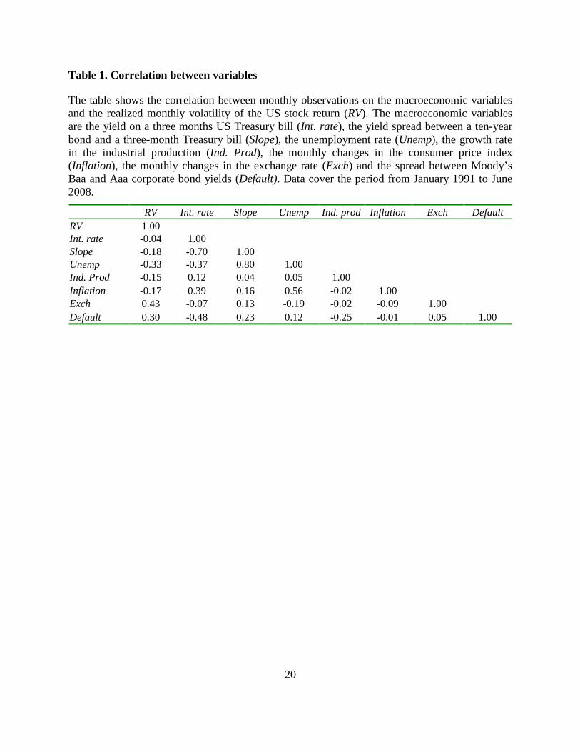
Table 1 shows the correlation between monthly observations on the macroeconomic variables

and the realized monthly volatility of the US stock return (RV). Interest rate, as expected, has a

high negative correlation with slope (-0.70). Further, the slope is higher when the unemployment

rate is high. Unemployment and inflation are also highly correlated during the selected time

span.

Table 2 shows the correlations between the principal components and the macroeconomic

variables. The first principal component (PC1) has a high correlation with most of the variables,

particularly with interest rate, slope, default rate, and unemployment (average correlation is

0.48). Since most of these variables are commonly used as a measure for business cycle we may

consider the variable PC1 as a proper proxy for the cycle. Similarly, we observe a relatively large

correlation between some variables i.e., inflation and interest rate with PC2. Other principal

components have either low correlations with the macroeconomic variables or only related to

one specific variable (such as PC3 and industrial production). We choose therefore only to

include PC1 and PC2 in the MIDAS equation. Figure 2 plots the monthly realized volatility of the

return, the macroeconomic variables, as well as the first two principal components constructed

based on the macroeconomic variables. A drastic fluctuation is observed in realized volatility

12

between the period 1997 till mid of 2002. This may indicate the effect of Asian crisis in 1998,

the burst of the dot-com bubble in 2000 and the September 11 incidence in 2001. The last

volatile period near 2007-2008 indicates the start of the recent financial crisis. We can find a

similar pattern in the movements of the PC1 series. It shows a declining trend in the beginning,

followed by a sharp increase in the values after the financial turmoil in 2001, which remains until

2003. An increasing trend around the period of 2007-2008 signals the start of the recent financial

crisis.

From the plot of PC2, we can observe a continuously increasing trend throughout the sample

period. The interest rate pattern is reversed of that for PC1 confirming the high negative

correlation between them (-0.78). Similarly, the default rate is high during financial crisis of

1998, 2001 and 2007 compared to other time periods. The growth rate in industrial production is

smooth besides some peak points near 1998. The exchange rate changes slightly around 2001,

otherwise it seems stable throughout the sample period. The inflation has an opposite behavior to

that of PC2, supporting their highly negative correlation (-0.83). Similarly, the unemployment

rate increases after the crisis of 2001 and remains high for the next couple of years. We can

observe an increasing trend in the unemployment rate after the recent financial crisis of 2008.

4.2. In-sample estimations

In Table 3, we present the estimated parameters of the in-sample fit for the first estimation

period, starting on January 01, 1991 and ending on December 31, 2003. The models are

estimated with the first two principal components and with all the individual economic variables

in the MIDAS equation. In order to save space we only report the results for PC1 and PC2. Most

of the parameters in the equations for returns and the short-term variance component (git) are

significant at the 5% level, indicating a clustering pattern in the short-term return variance.

Turning to the long-term component, we can see the RV is significant at the 5% level in all the

three models, while the weight w2 is only significant at the 10% level. In order to have the same

degree of smoothness for all the variables we use w2 estimated from the model with only RV,

when we augment the model with macroeconomic variables. The results show that the level of

PC1 is significant along with RV but not its variance. However, if we exclude RV from the

equation of the long-term component, both the levels and the variance of PC1 are significant. It

13

shows that RV captures the effect of the variance of PC1. RV is still significant at the 5% level

when we use PC2 as a macroeconomic variable. The parameter for the variance of PC2 is also

significant but at the 10% level. However, only the level of PC2 is found significant if we

exclude RV from the model. We may conclude that the joint effects of the economic variables,

captured by PC1 and PC2, contain some information about the driving force of stock market

return variance.

In Figure 3 we compare the estimated short-term, long-term and total variance from the

GARCH-MIDAS model where we only use the realized volatility in the MIDAS equation (RV

model). In the first part of the estimation window, despite some large peaks in the short-term

variance (possibly due to the Asian crises) the long-term variance is quite low. After 2000 we

observe a substantial increase in the long-term variance component, while the short-term

component is below the long-term component most of the time.

Figure 4 illustrates the estimated long-term component of the return variance given by the

MIDAS equation, for the first in-sample period. We compare the results from the RV model

with two alternative specifications, the RV model augmented with a macroeconomic variable and

a model which only includes the macroeconomic variable. In the first graph the macroeconomic

variables are represented by PC1, while in the second graph we present the estimated variances

with PC2. It shows that the estimated variance from the model RV+PC1 follows mostly that

from the RV model, while the PC1 model moves quite differently. Comparing all the three

models, it seems that the RV+PC1 model combines the two other models, where RV determines

the variations and PC1 affects mostly the level of the estimated variance. All the three models

give a relatively similar pattern, most of the time, when we use PC2 as the macroeconomic

variable.

4.3. Out-of-sample prediction

In this section, we analyze the ability of the GARCH-MIDAS model in forecasting the long-term

monthly variances, see equations (3) and (4), and the total daily variances, see equation (5). The

parameters are obtained using a rolling 10-year estimation window and are held constant during

the subsequent year. Our out-of-sample forecast covers the period from January 2004 to June

2008. We use three alternative MIDAS specifications: the RV model that only includes the

14

realized volatility of stock returns, the RV+Xl+Xv model that includes the realized return

volatility as well as the level and the variance of the economic variables, and finally the Xl+Xv

model with only the level and the variance of the economic variables. As our primary choice of

the macroeconomic variables in the GARCH-MIDAS model, we use the two first principal

components, PC1 and PC2. We use a ten-year estimation window and keep the parameters over

the subsequent year. The first estimation window starts in January 1994 and ends in December

2003. Table 4 reports the prediction performance of all the models using MSE and the DM test.

As a benchmark we estimate the GARCH (1,1) model, where we use monthly observations for

comparison with the GARCH-MIDAS long-term variance component and daily observations

when we compare it with the GARCH-MIDAS total variance. The estimated MSE is based on

the deviation between the variance forecasted and the realized variance, where the realized

monthly variances are estimated as the sum of daily squared returns in each month, and the

realized daily variances are the squared daily returns.

The left panel of Table 4 shows the results for the long-term variance component. The GARCH-

MIDAS model with RV+PC1 has lowest MSE values for monthly predictions. This result is

confirmed by the DM-test (In order to save space, we only report the DM-test when using the

traditional GARCH and GARCH-MIDAS as the benchmark models). The model RV+ PC1

significantly outperforms both the GARCH model and the RV model in the long-term variance

prediction. The GARCH-MIDAS model without any economic variable performs better than

GARCH but the difference between the models forecast is not statistically significant. The

models with PC1 and PC2 alone, as a long-term variance driving factor, perform very poorly and

are significantly worse than both GARCH and RV model.

In the right panel of the table, we display the findings from daily variance predictions. The

RV+PC1 model still performs better than the other models, but the differences are very small and

statistically insignificant. In fact all the models perform better than the GARCH model.

In figure 5, we plot the results of the regression of the realized volatility on the predicted

variance. In general, if the predicted variance has some information about the future realized

volatility, then the slope parameter should be significantly different from zero. Furthermore, for

an unbiased prediction we expect the intercept parameter to be zero and the slope parameter to be

15

equal to one. The first graph shows the t-statistics for the intercept for both daily and monthly

variance predictions, and the slope parameters for daily and monthly variance predictions are

presented in the second and third diagrams, respectively. In accordance to the results above, the

RV+PC1 model shows a very strong ability in forecasting both long-term (monthly) and total

(daily) variances; it has a very close to zero intercept and a close to one slope estimations in

both predictions. None of the other models share these properties for both predictions, for

example the RV model performs well at the daily prediction but its slope is not significantly

different from zero in the monthly prediction.

All in all, our out-of-sample analysis shows that adding proper macroeconomic information,

measured by PC1, to the long-term variance component of the GARCH-MIDAS model

significantly enhances the prediction ability of the model. Now, it is interesting to analyze the

forecasting ability of the different macroeconomic variables, separately. Figure 6 plots the DM-

test result of the RV+Xl+Xv model, using individual macroeconomic variables and the two

principal components, and that of the RV model. The GARCH (1, 1) model is used as the

benchmark to compute the test statistics. According to the figure, all the statistics are negative,

which implies that all the models give a lower forecast error than the GARCH model, in both

monthly and daily predictions. However, the test is only significant for monthly predictions and

for three cases, i.e. the specifications with PC1, interest rate, and default. Since the both interest

rate and default are highly correlated with PC1, the strong out-of-sample performance of the

model with PC1, can to a large extent be related to these two variables.

5. Conclusion

In this paper, we have used the GARCH-MIDAS approach to forecast future variances. To

estimate the long-term component of the variance, in addition to the smoothed realized volatility

we use information from macroeconomic variables. A principal component approach is

employed to combine the information from a large number of variables, which include interest

rate, unemployment rate, term premium, inflation rate, exchange rate, default rate, industrial

production growth rate. We use a rolling window to estimate the parameters of the model and to

make forecast for out-of-sample variances. We compare the forecasting ability of GARCH-

MIDAS models with the traditional GARCH model.

16

Our findings show that the GARCH-MIDAS model constitutes a better forecast than the

traditional GARCH model. We show that including the low-frequency (monthly)

macroeconomic information not only significantly enhances the forecasting ability of the model

for the long-term (monthly) variance, it also improves the prediction ability of the model for

high-frequency (daily) variances. However, the latter result is not statistically significant based

on the DM-test. The GARCH-MIDAS model that includes the first principal component

outperforms all other specifications. The strong performance of the first principal component

may be motivated by its close connection to the variables short term interest rate and the default

rate, which makes the first principal component a good proxy of the business cycle.

The paper contributes to existing literature by (1) augmenting the long-term component (MIDAS

equation) with macroeconomic variables and (2) investigating the forecasting ability of the

GARCH-MIDAS model.

17

References

Alper, C. E., S. Fendoglu, and B. Saltoglu (2008). Forecasting Stock Market Volatilities Using

MIDAS Regression: An Application to the Emerging Markets. MPRA Paper No. 7460.

Andersen, T. and Bollerslev, T. (1998). Answering the Skeptics: Yes, Standard Volatility Models

Do Provide Accurate Forecasts, International Economic Review, 39, 885-905.

Anderson, T., T. Bollerslev, and F. Diebold (2007). Roughing It Up: Including Jump Component

in the Measurement, Modeling and Forecasting of Return Volatility. The Review of Economics

and Statistics, 89,701-720.

Andreaou, E., E. Ghysels, and A. Kourtellos (2010a). Regression Models with Mixed Data

Sampling Frequencies. Journal of Econometrics, in-press.

Bai, J., E. Ghysels, and J. Wright (2009). State space models and MIDAS regression. Working

Paper, NY Fed, UNC and John Hopkins.

Brandt, M. W. and Kang, Q. (2002). On the relationship between the conditional mean and

volatility of stock returns: A latent VAR approach. The Wharton School.

Brooks, C. and G. Persand (2003), The Effect of Asymmetries on Stock Index Return Value at

Risk Estimates, Journal of Risk Finance, 4, 29-42.

Chen, X., and E. Ghysels (2007). News –Good or Bad- and Its Impact on Multiple Horizons.

Working Paper, NC-Chapel Hill.

Chen, X., and E. Ghysels (2009). News – good or bad – and its impact on predicting future

volatility. Review of Financial Studies (forthcoming).

Chernov, M., Gallant, R., Ghysels, E. and Tauchen, G. (2003), Alternative models for stock price

dynamics, Journal of Econometrics, 116, 225-257.

Clements, M. P., and Galavao, A. B. (2006) Macroeconomic Forecasting with mixed Frequency

Data: Forecasting US output growth and inflation. Warwick Economic Research Paper No. 773.

University of Warwick.

Diebold, F. and Mariano, S. (1995). Comparing Predictive Accuracy, Journal of Business &

Economic Statistics, 13, 253-63.

18

Ding, Z. and Granger, C. (1996), Modeling volatility persistence of speculative returns: A new

approach. Journal of Econometrics 73, 185-215.

Engle, R., and Lee, G. (1999), A permanent and transitory component model of stock return

volatility. In ed. R.F. and H. White, Cointegration, Causality, and Forecasting: A Festschrift in

Honor of Clive W.J. Granger, Oxford University press, 475-497.

Engle, R., E. Ghysels, and B. Sohn. (2009). Stock Market Volatility and Macroeconomic

Fundamentals, Working Paper.

Forsberg, L., and E. Ghysels (2006). Why do absolute returns predict volatility so well? Journal

of Financial Econometrics, 6, 31-67.

Ghysels, E., P. Santa-Clara, and R. Valkanov (2004). The MIDAS touch: Mixed Data Sampling

Regression. Discussion Paper UNC and UCLA.

Ghysels, E., A. Sinko, and R. Valkanov (2006). MIDAS regression: Further results and new

directions. Econometric Reviews, 26, 53-90.

Ghysels, E., A. Sinko, and R. Valkanov (2009). Granger Causality Tests with Mixed Data

Frequencies. Discussion Paper, UNC.

Glosten, L. R., Jagannathan, R. and Runkle, D. E. (1993). On the relationship between the

expected value and the volatility of the nominal excess return on stocks, Journal of Finance 48,

1779–1801.

Goffe, W.L., Ferrier, G.D., Rogers, J. (1994). Global optimization of statistical functions with

simulated annealing, Journal of Econometrics, 60, 65–99.

Hamilton, J. D., and G, Lin. (1996). Stock Market Volatility and the Business Cycle, Journal of

Applied Econometrics, 11, 573-593.

Hansen, P.R. (2005). A test for superior predictive ability, Journal of Business and Economic

Statistics, 23, 365-380.

Kotze, G. L. (2007). Forecasting Inflation with High Frequency Asset Price Data. Working

Paper. University of Stellenbosch.

19

Perez-Quiros, G. and Timmermann, A. (2000), ‘’Firm size and cyclical variations in stock

returns’’, Journal of Finance, 55, 1229–1262.

Schwert, G. W., (1989). Why Does Stock Market Volatility Change over Time?, Journal of

Finance, 44, 1115-1153.

Tay, A. S. (2007). Mixed Frequencies: Stock Returns as a Predictor of real Output Growth.

Discussion Paper, SMU.

Whitelaw, R. (1994), Time variations and covariations in the expectation and volatility of sock

returns, Journal of Finance 49, 515–541.

20

Table 1. Correlation between variables

The table shows the correlation between monthly observations on the macroeconomic variables and the realized monthly volatility of the US stock return (RV). The macroeconomic variables are the yield on a three months US Treasury bill (Int. rate), the yield spread between a ten-year bond and a three-month Treasury bill (Slope), the unemployment rate (Unemp), the growth rate in the industrial production (Ind. Prod), the monthly changes in the consumer price index (Inflation), the monthly changes in the exchange rate (Exch) and the spread between Moody’s Baa and Aaa corporate bond yields (Default). Data cover the period from January 1991 to June 2008.

RV Int. rate Slope Unemp Ind. prod Inflation Exch Default RV 1.00 Int. rate -0.04 1.00 Slope -0.18 -0.70 1.00 Unemp -0.33 -0.37 0.80 1.00 Ind. Prod -0.15 0.12 0.04 0.05 1.00 Inflation -0.17 0.39 0.16 0.56 -0.02 1.00 Exch 0.43 -0.07 0.13 -0.19 -0.02 -0.09 1.00 Default 0.30 -0.48 0.23 0.12 -0.25 -0.01 0.05 1.00

21

Table 2. The correlation of principal components with the macroeconomic variables

The table shows the correlation between the macroeconomic variables with the principal components (PC) constructed based on these variables. The macro economic variables are the yield on a three months US Treasury bill (Int. rate), the yield spread between a ten-year bond and a three-month Treasury bill (Slope), the spread between Moody’s Baa and Aaa corporate bond yields (Default), the monthly changes in the exchange rate (Exch), the monthly changes in the consumer price index (Inflation), the growth rate in the industrial production (Ind. Prod) and the unemployment rate (Unemp). Data cover the period from January 1991 to June 2008.

Int. rate Slope Unemp Ind. prod Inflation Exch Default Pc1 -0.78 0.93 0.83 -0.10 0.21 0.02 0.49 Pc2 -0.54 -0.06 -0.53 -0.28 -0.83 0.36 0.43 Pc3 0.14 -0.25 -0.02 -0.82 0.33 -0.27 0.44 Pc4 0.19 0.09 -0.03 -0.16 0.33 0.89 0.00 Pc5 0.10 -0.16 -0.09 0.46 0.17 0.01 0.61 Pc6 -0.19 -0.14 -0.02 0.02 0.12 0.01 -0.06 Pc7 0.02 -0.12 0.17 0.00 -0.09 0.04 0.01

22

Table 3. Estimated parameters of the GARCH-MIDAS model

The table shows the estimated parameters of the GARCH-MIDAS model with different specifications of the MIDAS equation. The first row of the table presents the results of the model with only the realized volatility (RV) of returns in the MIDAS equation, while the rest rows of the table present the estimated parameters when we also include the level and the variance of the economic variables, Xl and Xv respectively, in the MIDAS equation. We only present the results obtained for the first and the second principal components constructed based on seven macroeconomic variables. Data cover the first estimation period starting in January 1991 and ending in December 2003.

mu alpha beta m RV level var w2 RV 0.072** 0.086** 0.887** -0.634** 0.031** 2.677*

PC1 RV+ Xl+Xv 0.075** 0.090** 0.861** -0.814** 0.034** -0.219** -2.004

Xl+Xv 0.072** 0.071** 0.924** 0.848 -0.438** -12.983**

PC2 RV+ Xl+Xv 0.075** 0.099** 0.860** -1.143** 0.038** 0.107 2.917*

Xl+Xv 0.072** 0.082** 0.900** -0.115 -0.295** 2.677

23

Table 4. Comparisons of the out-of-sample prediction errors

The table shows the results of the estimated mean square error (MSE) and DM-test for the out-of-sample performance of the different models in predicting daily and monthly variances. We use three alternative specifications in the MIDAS equation, a model that includes only the realized volatility of stock returns (RV model), a model that includes the realized return volatility as well as the level and the variance of the economic variables (RV+Xl+Xv), and finally a model with only the level and the variance of the economic variables (Xl+Xv). The left panel shows the results for the long-term variance component, τ in equations (3) and (4), while right panel shows the results for the conditional daily total variance (see equation (5)). The results of the GARCH-MIDAS are compared with corresponding GARCH estimations. As the macro variables we use the two first principal components, PC1 and PC2, in the MIDAS equation. We use a ten-year estimation window and keep the parameters over the subsequent year. The first estimation window starts in January 1994 and ends in December 2003. The realized monthly variances are estimated as the sum of daily squared returns in each month, while for the realized daily variances we use the squared daily returns. Out-of-sample forecasts cover the period from January 2004 to June 2008. The minus (plus) sign in each cell indicates that the model given in the row performs better (worse) than the model given in the column. An asterisk implies a significant difference in the performance.

Long term variance Total variance MSE GARCH RV model MSE GARCH RV model

GARCH 174.18 + 1.71 +

RV model 171.53 - 1.69 -

RV+PC1 133.19 -* -* 1.68 - -

RV+PC2 225.28 + + 1.69 - -

PC1 219.98 +* +* 1.70 - +

PC2 233.32 +* +* 1.70 - +

24

Figure 1. The weights and the number of lags in GARCH-MIDAS The upper graph shows the behavior of weights as the function of the number of lags using different values for w1 and w2. We select two alternative values for w1 (1 and 2) and two values for w2 (4 and 8). In the lower graph, we plot the maximized value of log likelihood function of the GARCH-MIDAS model with different lag values. The long term component (MIDAS equation) includes only the realized return volatility.

Weights and Lags

0

0.05

0.1

0.15

0.2

0.25

1 3 5 7 9 11 13 15 17 19 21 23 25 27 29 31 33 35

Lags

Wei

gh

ts

1,4

1,8

2,4

2,8

Lags and Likelihhod functions

-3800

-3700

-3600

-3500

-3400

-3300

-3200

0 20 40 60 80

Lags

Lik

elih

oo

d f

un

ctio

ns

Likelihhod Fs

25

Figure 2. Plot of the realized volatility and the economic variables

The figure illustrates the monthly realized volatility of the return and movements of the selected macroeconomic variables, as well as the first principal component constructed based on the macroeconomic variables. The data ranges from January 1991 to June 2008.

-2.50

-2.00

-1.50

-1.00

-0.50

0.00

0.50

1.00

1.50

2.00

2.50

Industrial production

0.00

20.00

40.00

60.00

80.00

100.00

120.00

140.00

160.00

RV

0.00

1.00

2.00

3.00

4.00

5.00

6.00

7.00

8.00

Interest rate

0.00

0.20

0.40

0.60

0.80

1.00

1.20

1.40

1.60

Defualt rate

0.00

1.00

2.00

3.00

4.00

5.00

6.00

7.00

8.00

9.00

Unemployment rate

0.00

1.00

2.00

3.00

4.00

5.00

6.00

Inflation

0.00

20.00

40.00

60.00

80.00

100.00

120.00

Exchange rate

-3.00

-2.00

-1.00

0.00

1.00

2.00

3.00

PC1

-4.00

-3.00

-2.00

-1.00

0.00

1.00

2.00

3.00

PC2

-2.00

-1.00

0.00

1.00

2.00

3.00

4.00

Slope

26

Figure 3. Comparison of the long-term , short-term and total variance

The figure illustrates the long-term, short-term and total variances estimated by the GARCH-MIDAS model. The MIDAS equation only includes the realized volatility of stock returns (RV model). The estimation period covers the period from January 1991 to December 2003, while a sample of 36 monthly observations have been used to estimate the exponentially moving average of the realized volatility in the MIDAS equation.

0

1

2

3

4

5

6

7

8

1994 1994 1995 1996 1997 1998 1999 2000 2001 2002 2003

RV ModelTotalShortLong

27

Figure 4. Estimated long-term variance

The figure illustrates the estimated long-term variance, τt, based on three alternative specifications of the MIDAS equation, a model that includes only the realized volatility of stock returns (RV), a model that includes the realized return volatility as well as the level and the variance of the economic variables (RV+Xl+Xv), and finally a model with only the level and the variance of the economic variables (Xl+Xv). We illustrate the results for the first two principal components constructed based on seven macroeconomic variables. The estimation period covers the period from January 1991 to December 2003, while a sample of 36 monthly observations have been used to estimate the exponentially moving average of the included variables in the MIDAS equation.

0

20

40

60

80

100

120

1994 1995 1996 1997 1998 1999 2000 2001 2002 2003

PC1RV model

RV+PC1

PC1

0

10

20

30

40

50

60

70

1994 1995 1996 1997 1998 1999 2000 2001 2002 2003

PC2RV model

RV+PC2

PC2

28

Figure 5. Regression of the realized volatilities on the predicted variances

The figure plots the results of the estimated parameters from the regression of the realized volatility on the predicted variance. The first figure plots the t-statistics for the intercept and the second and third figures give the slope parameters for monthly and daily variance prediction, respectively, and the related 95% confidence intervals. We use three alternative MIDAS specifications: RV includes only the realized volatility of stock returns, RV+Xl+Xv includes the realized return volatility and the level and the variance of the economic variables, Xl+Xv contains only the level and the variance of the economic variables. As economic variables, we use two first principal components, PC1 and PC2, in the MIDAS equation. The results of the GARCH-MIDAS are compared with corresponding GARCH estimations. The realized monthly volatility is estimated as the sum of daily squared returns in each month, while for the realized daily volatility is computed as the squared daily return.

0.0

0.5

1.0

1.5

Garch RV RV+PC1 RV+PC2 PC1 PC2

95% confidence interval for slope coefficientDaily variance

-0.5

0.0

0.5

1.0

1.5

2.0

2.5

Garch RV RV+PC1 RV+PC2 PC1 PC2

t-values of the estimated intercept Monthly

Daily

-1.0

0.0

1.0

2.0

3.0

4.0

Garch RV RV+PC1 RV+PC2 PC1 PC2

95% confidence interval for slope coefficientMonthly variance

29

Figure 6. DM-test of the individual macrovariables

The figure shows t-values of the DM test for the out-of-sample performance of the different models in predicting daily and monthly variances. It indicates the contribution of each macroeconomic variable, PC1 and PC2 in order to improve the prediction of long-term variance. We use two alternative specifications in MIDAS equation, a model that includes only the realized volatility of stock returns (RV model), a model that includes the realized return volatility as well as the level and the variance of the economic variables (RV+Xl+Xv).

-3

-2

-1

0

t-values of the DM-test

Monthly

Daily