A Gas Dynamics - Springer978-3-540-27321-9/1.pdfA Gas Dynamics The nature of stars is complex and...

A

Gas Dynamics

The nature of stars is complex and involves almost every aspect of modernphysics. In this respect the historical fact that it took mankind about half acentury to understand stellar structure and evolution (see Sect. 2.2.3) seemsquite a compliment to researchers. Though this statement reflects the advancesin the first half of the 20th century it has to be admitted that much of stellarphysics still needs to be understood, even now in the first years of the 21stcentury. For example, many definitions and principles important to the physicsof mature stars (i.e., stars that are already engaged in their own nuclearenergy production) are also relevant to the understanding of stellar formation.Though not designed as a substitute for a textbook about stellar physics, thefollowing sections may introduce or remind the reader of some of the verybasic but most useful physical concepts. It is also noted that these conceptsare merely reviewed, not presented in a consistent pedagogic manner.

The physics of clouds and stars is ruled by the laws of thermodynamicsand follows principles of ideal, adiabatic, and polytropic gases. Derivatives ingas laws are in many ways critical in order to express stability conditions forcontracting and expanding gas clouds. It is crucial to properly define gaseousmatter. In the strictest sense a monatomic ideal gas is an ensemble of thesame type of particles confined to a specific volume. The only particle–particleinteractions are fully elastic collisions. In this configuration it is the number ofparticles and the available number of degrees of freedom that are relevant. Anensemble of molecules of the same type can thus be treated as a monatomicgas with all its internal degrees of freedom due to modes of excitation. Ionizedgases or plasmas have electrostatic interactions and are discussed later.

A.1 Temperature Scales

One might think that a temperature is straightforward to define as it is aneveryday experience. For example, temperature is felt outside the house, insideat the fireplace or by drinking a cup of hot chocolate. However, most of what is

258 A Gas Dynamics

experienced is actually a temperature difference and commonly applied scalesare relative. In order to obtain an absolute temperature one needs to invokestatistical physics. Temperature cannot be assigned as a property of isolatedparticles as it always depends on an entire ensemble of particles in a specificconfiguration described by its equation of state. In an ideal gas, for example,temperature T is defined in conjunction with an ensemble of non-interactingparticles exerting pressure P in a well-defined volume V . Kinetic temperatureis a statistical quantity and a measure for internal energy U . In a monatomicgas with Ntot particles the temperature relates to the internal energy as:

U = 32Ntotk T (A.1)

where k = 1.381× 10−16 erg K−1.The Celsius scale defines its zero point at the freezing point of water and

its scale by assigning the boiling point to 100. Lord Kelvin in the mid-1800sdeveloped a temperature scale which sets the zero point to the point at whichthe pressure of all dilute gases extrapolates to zero from the triple point ofwater. This scale defines a thermodynamic temperature and relates to theCelsius scale as:

T = TK = TC + 273.15o (A.2)

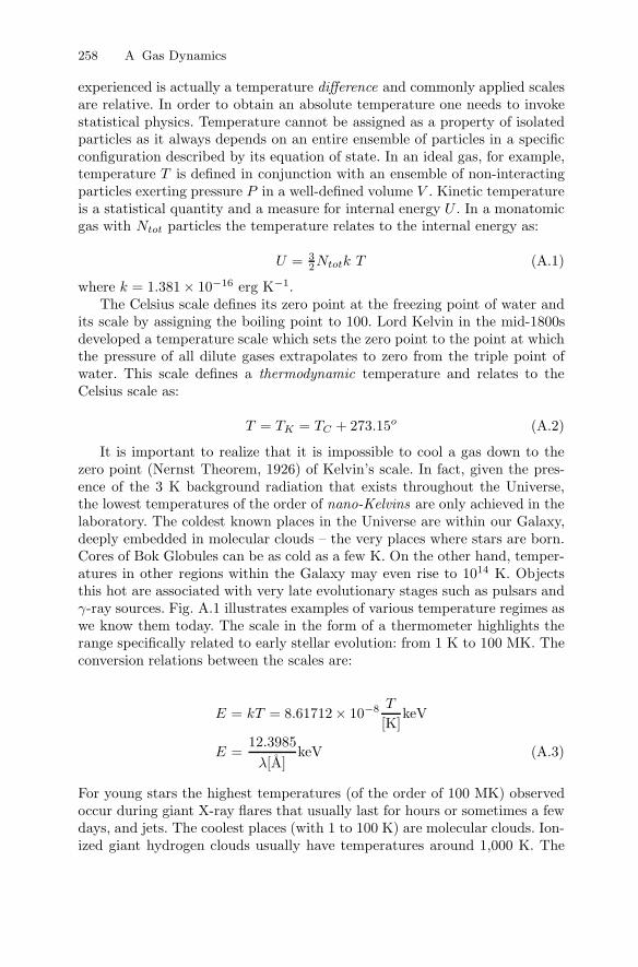
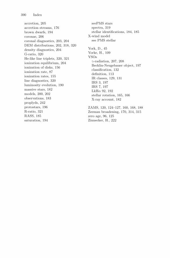
It is important to realize that it is impossible to cool a gas down to thezero point (Nernst Theorem, 1926) of Kelvin’s scale. In fact, given the pres-ence of the 3 K background radiation that exists throughout the Universe,the lowest temperatures of the order of nano-Kelvins are only achieved in thelaboratory. The coldest known places in the Universe are within our Galaxy,deeply embedded in molecular clouds – the very places where stars are born.Cores of Bok Globules can be as cold as a few K. On the other hand, temper-atures in other regions within the Galaxy may even rise to 1014 K. Objectsthis hot are associated with very late evolutionary stages such as pulsars andγ-ray sources. Fig. A.1 illustrates examples of various temperature regimes aswe know them today. The scale in the form of a thermometer highlights therange specifically related to early stellar evolution: from 1 K to 100 MK. Theconversion relations between the scales are:

E = kT = 8.61712× 10−8 T

[K]keV

E =12.3985

λ[A]keV (A.3)

For young stars the highest temperatures (of the order of 100 MK) observedoccur during giant X-ray flares that usually last for hours or sometimes a fewdays, and jets. The coolest places (with 1 to 100 K) are molecular clouds. Ion-ized giant hydrogen clouds usually have temperatures around 1,000 K. The

A.1 Temperature Scales 259

1,000

100

1,000

10,000

100,000

1

10

100

10,000

100,000

1 Million

10 Million

100 Million

0.1

0.01

0.001

Kelvin eV Angstrom

100 billion

10 billion

100 million

1 billion

10 million

10 million

1 million

1

10

100

1,000

10,000

100,000

1 million

0.0001

0.001

0.01

0.1

1

10

Infra−red

Sub−mm

rays

Gam

ma−

X−rays

Radio

violetU

ltra−

Optical

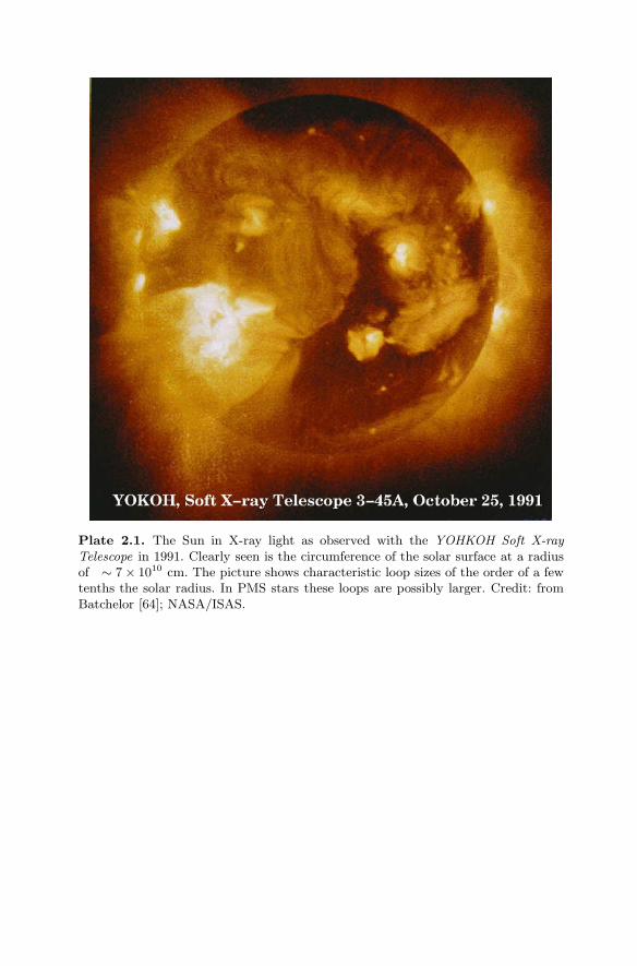
Fig. A.1. The temperature scale in the Universe spans over ten orders of magnituderanging from the coldest cores of molecular clouds to hot vicinities of black holes.The scale highlights the range to be found in early stellar evolution, which roughlyspans from 10 K (e.g., Barnard 68) to 100 MK (i.e. outburst and jet in XZ Tauriand HH30, respectively). Examples of temperatures in-between are ionized hydrogenclouds (e.g., NGC 5146, Cocoon Nebula), the surface temperatures of stars (e.g., ourSun in visible light), plasma temperatures in stellar coronal loops (e.g., our Sun inUV light), magnetized stars (i.e., hot massive stars at the core of the Orion Nebula).The hottest temperatures are usually found at later stages of stellar evolution insupernovas or the vicinity of degenerate matter (e.g., magnetars). Credits for insets:NASA/ESA/ISAS; R. Mallozzi, Burrows et al. [136], Bally et al. [52], Schulz etal. [761].

temperatures of stellar photospheres range between 3,000 and 50,000 K. Instellar coronae the plasma reaches 10 MK, almost as high as in stellar coreswhere nuclear fusion requires temperatures of about 15 MK. The temperaturerange involved in stellar formation and evolution thus spans many orders ofmagnitudes. In stellar physics the high temperature is only topped by tem-peratures of shocks in the early phases of a supernova, the death of a massivestar, or when in the vicinity of gravitational powerhouses like neutron starsand black holes.

260 A Gas Dynamics

A.2 The Adiabatic Index

The first relation one wants to know about a gaseous cloud is its equation ofstate, which is solely based on the first law of thermodynamics and representsconservation of energy:

dQ = dU + dW (A.4)

where the total amount of energy absorbed or produced dQ is the sum of thechange in internal energy dU and the work done by the system dW. In anideal gas where work dW = PdV directly relates to expansion or compressionand thus a change in volume dV against a uniform pressure P , the equationof state is:

PV = NmRT = nkT (A.5)

where R = 8.3143435×107 erg mole−1 K−1, Nm is the number of moles, and nis the number of particles per cm3. The physics behind this equation of state,however, is better perceived by looking at various derivatives under constantconditions of involved quantities. For example, the amount of heat necessaryto raise the temperature by one degree is expressed by the heat capacities:

Cv =(

dQ

dT

)V

and Cp =(

dQdT

)P

(A.6)

where d/dT denotes the differentiation with respect to temperature and theindices P and V indicate constant pressure or volume. The ratio of the twoheat capacities:

γ = CP /CV (A.7)

is called the adiabatic index and has a value of 5/3 or 7/5 depending onwhether the gas is monatomic or diatomic. For polyatomic gases the ratiowould be near 4/3 (i.e., if the gas contains significant amounts of elementsother than H and He or a mix of atoms, molecules, and ions). The more inter-nal degrees of freedom to store energy that exist, the more CP is reduced, al-lowing the index to approach unity. A mix of neutral hydrogen with a fractionof ionized hydrogen is in this respect no longer strictly monatomic, becauseenergy exchange between neutrals and ions is different. Similarly, mixes of Hand He and their ions are to be treated as polyatomic if the ionization frac-tions are large. Deviations from the ideal gas assumption scale with n2/V 2,which, however, in all phases of stellar formation is a very small number. Thusthe ideal gas assumption is quite valid throughout stellar evolution.

A very important aspect with respect to idealized gas clouds is the case inwhich the radiated heat is small. For many gas clouds it is a good approxima-tion to assume that no heat is exchanged with its surroundings. The changesin P, T , and V in the adiabatic case are then:

A.3 Polytropes 261

PV γ = const; TV γ−1 = const; and TP (1−γ)/γ) = const (A.8)

Together with equations A.4 and A.5 these relations lead to a set of three adia-batic exponents by requiring that dQ = 0. The importance of these exponentshad been realized by Eddington in 1918 and Chandrasekhar in 1939 [699].They are defined as:

Γ1 = −(

dlnPdlnV

)ad

=(

dlnPdlnρ

)ad

(A.9)

Γ2

(Γ2 − 1)=

(dlnPdlnT

)ad

(A.10)

and

Γ3 − 1 = −(

dlnTdlnV

)ad

(A.11)

In the classical (non-adiabatic) limit for a monatomic gas with no internaldegrees of freedom, the three exponents are the same and equal to 5/3. Fora typical non-interacting gas the specific internal energy U (internal energyper unit mass) is proportional to P/ρ (where ρ is the mass density). Thuspressure of such a system is related to density by:

P = Kργ (A.12)

where K is a proportionality factor determined by the gas considered and γ isgenerally Γ1 . These exponents carry crucial information about the stability ofthe system against various types of perturbations. In the case of an isothermalcloud, it is primarily the first adiabatic exponent that defines the stability ofa gas against external forces (such as gravity), and changes in Γ2 and Γ3 arenegligible. The latter only have more significance once convection occurs andif processes are strongly non-isothermal.

A.3 Polytropes

Stellar interiors are frequently characterized by polytropic processes, wherethe adiabatic condition of dQ = 0 is now substituted by a constant thermalcapacity:

C =dQ

dT= const. > 0 and γ′ =

Cp − CCv − C

(A.13)

With the (A.12) the polytropic equation of state has then the index γ′. Thepolytropic index is then defined as n = 1/(γ′ − 1).

262 A Gas Dynamics

A.4 Thermodynamic Equilibrium

For an ideal gas of temperature T of n particles of a certain kind there arevarious excited states. Atoms in an excited state i with an excitation energy χi

distribute relative to their ground states o following the Boltzmann formula:

ni

no=

gi

goe−χi/kT (A.14)

where gi and go are the statistical weights describing the degeneracy of states.However, at larger temperatures ground states are increasingly depleted. Inthe extreme case that all ground states are depleted no is substituted by thetotal number of states n, and go by the partition function g =

∑i gie

χi/kT .The temperature T is then the equilibrium temperature. If the gas consists ofa mix of many atoms and molecules in various states of excitation, all particlespecies have the same temperature in thermodynamic equilibrium. However,such a global equilibrium may not be applicable in molecular clouds and starswhere temperatures may depend on spatial coordinates. Here the concept ofthermal equilibrium is still valid for small volume elements. This is then calledlocal thermodynamic equilibrium (LTE).

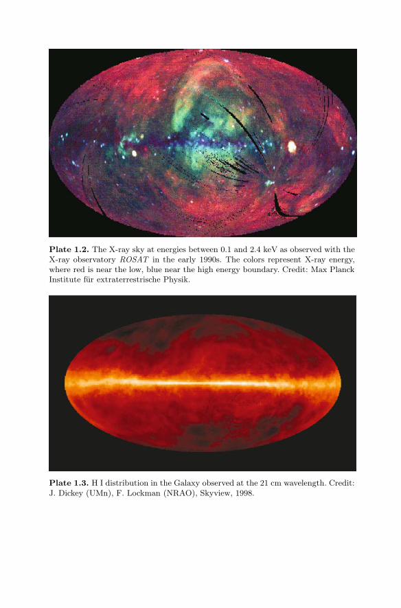
In thermal equilibrium every process occurs at the same rate as its inverseprocess, meaning there is as much absorption of photons as there is emission.Under such conditions the intensity of the radiation field can be described as:

Bν(T ) =2hν3

c2

1ehν/kT − 1

(A.15)

It was G. Kirchhoff (1860) and M. Planck (1900) who realized that the inten-sity of this blackbody radiation is a universal function of T and ν. The energyof the photon is hν, where h is Planck’s constant = 6.625×1027 erg s. The twolimiting cases are Wien’s law ( hν

kT 1) and Rayleigh–Jeans law ( hνkT 1).

The mean photon energy in local thermal equilibrium is equivalent to thetemperature of the radiating body by:

< hν >= 2.7012kT (A.16)

The energy and wavelength scales in Fig. A.1 are calculated through thisequivalency. Integration of (A.15) yields the total radiation flux F of a black-body radiator, which J. Stefan (1884 experimentally) and L. Boltzmann (1886theoretically) determined as:

F =∫ ∞

0

Bν(T )dν = σT 4 (A.17)

where σ = 5.67 × 10−5 erg cm−2 s−1 K−4.

A.5 Gravitational Potential and Mass Density 263

101010101010104 6 8 10 12 14 16

−5

−15

−2010

10

10−10

10

100

Radio IR UV

1K

10K

100 K5,000 K

40,000 K

O

Ray

leig

h−J

ean

s la

w

Wien

lawB[e

rg s

c

m

Hz

s

ter

]

ν −1

−2−1

−1

λ

10 10 10 10 10 10 106 4 2 0 −2 −6 −8

ν [Hz]

[ cm ]

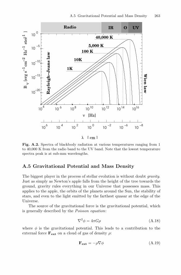
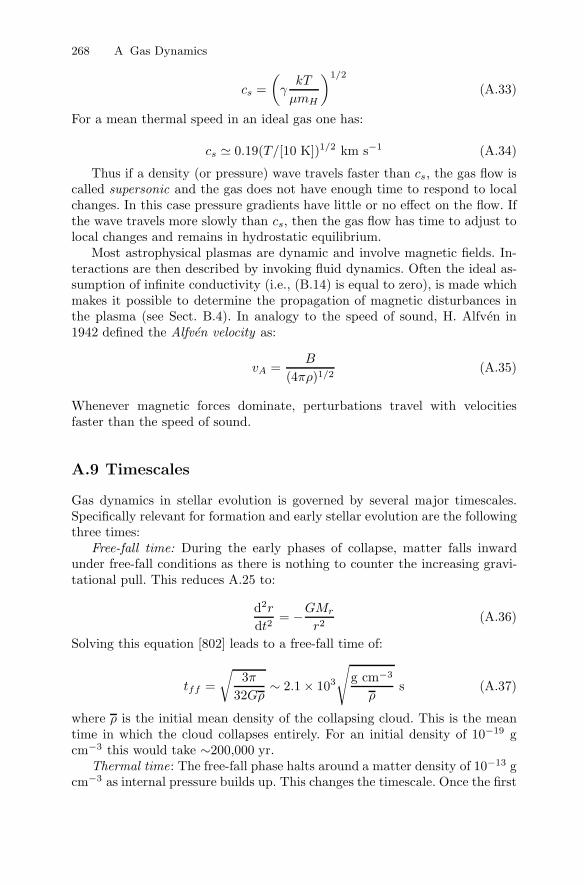
Fig. A.2. Spectra of blackbody radiation at various temperatures ranging from 1to 40,000 K from the radio band to the UV band. Note that the lowest temperaturespectra peak is at sub-mm wavelengths.

A.5 Gravitational Potential and Mass Density

The biggest player in the process of stellar evolution is without doubt gravity.Just as simply as Newton’s apple falls from the height of the tree towards theground, gravity rules everything in our Universe that possesses mass. Thisapplies to the apple, the orbits of the planets around the Sun, the stability ofstars, and even to the light emitted by the farthest quasar at the edge of theUniverse.

The source of the gravitational force is the gravitational potential, whichis generally described by the Poisson equation:

∇2φ = 4πGρ (A.18)

where φ is the gravitational potential. This leads to a contribution to theexternal force Fext on a cloud of gas of density ρ:

Fext = −ρ∇φ (A.19)

264 A Gas Dynamics

R R e

r

θ

Μ

m

pR

Ω

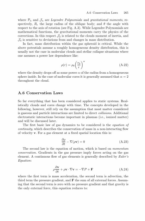
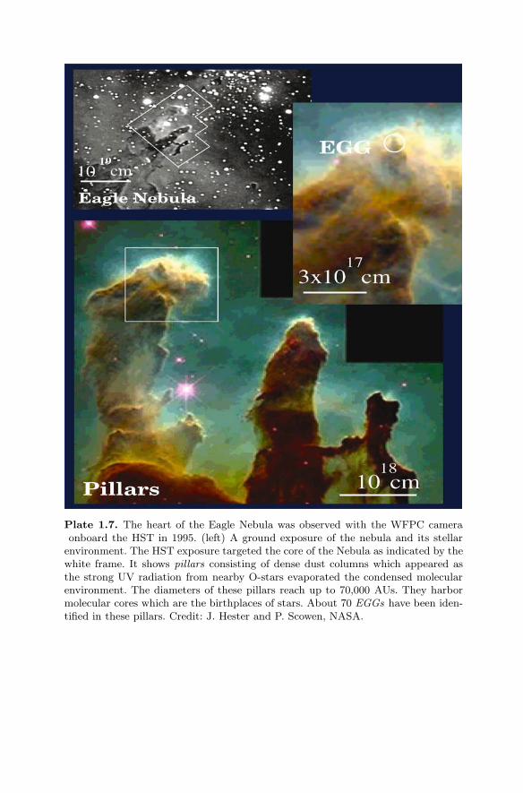
Fig. A.3. Geometry for an oblique rotator with obliqueness (Re − Rp)/Re.

In the case of spherical symmetry, where mass is distributed such that the totalgravitational potential only depends on the distance r towards the geometricalcenter of the mass distribution, φ can be expressed analytically as:

φ(r) = −GMr

r(A.20)

where Mr is the enclosed mass within a sphere of radius r. In fact, sphericalsymmetry is the only case where an exact analytical evaluation of the gravita-tional potential is possible. Thus the situation changes dramatically once thereare deviations from spherical symmetry. Imagine an isothermal gas cloud withno forces acting other than internal pressure and the gravitational force. Onceit rotates it redistributes itself into a more oblique shape breaking the symme-try (see Fig. A.3). This means that the gravitational potential now maintainsa cylindrical symmetry and an azimuthal angle θ dependence is added. Inthe case of slow rotation, the gravitational potential can be expanded as aninfinite series of the form:

φ(r, θ) = −GM

r

⎧⎪⎪⎩1 −(

Re

r

)2

J2P2(cos θ)

−(

Re

r

)4

J4P4(cos θ) − ...

⎫⎪⎪⎭ (A.21)

A.6 Conservation Laws 265

where Pn and Jn are Legendre Polynomials and gravitational moments, re-spectively, Re the large radius of the oblique body; and θ the angle withrespect to the axis of rotation (see Fig. A.3). While Legendre Polynomials aremathematical functions, the gravitational moments carry the physics of thecorrections. In this respect J2 is related to the clouds moment of inertia, andJ4 is sensitive to deviations from and changes in mass distribution.

In fact, mass distribution within the gas spheroid is critical. While theabove potentials assume a roughly homogeneous density distribution, this isusually not the case in molecular clouds and stellar collapse situations whereone assumes a power law dependence like:

ρ(r) = ρ0

(r0

r

)α

(A.22)

where the density drops off as some power α of the radius from a homogeneoussphere inside. In the case of molecular cores it is generally assumed that α = 2throughout the cloud.

A.6 Conservation Laws

So far everything that has been considered applies to static systems. Real-istically clouds and cores change with time. The concepts developed in thefollowing, however, still rely on the assumption that most matter consideredis gaseous and particle interactions are limited to direct collisions. Additionalelectrostatic interactions become important in plasmas (i.e., ionized matter)and will be discussed later.

The first basic law of gas dynamics to be considered is the equation ofcontinuity, which describes the conservation of mass in a non-interacting flowof velocity v. For a gas element at a fixed spatial location this is:

∂ρ

∂t−∇(ρv) = 0 (A.23)

The second law is the equation of motion, which is based on momentumconservation. Gradients in the gas pressure imply forces acting on the gaselement. A continuous flow of gas elements is generally described by Euler’sEquation:

ρ∂v∂t

+ ρv · ∇v = −∇P + F (A.24)

where the first term is mass acceleration, the second term is advection, thethird term the pressure gradient, and F the sum of all external forces. Assum-ing that the second term is zero with no pressure gradient and that gravity isthe only external force, this equation reduces to:

266 A Gas Dynamics

d2r

dt2= −GMr

r2= −4

3πGρr (A.25)

assuming the uniform sphere ρ here is an average density defined by Mr =(4/3)πr3ρ. This is the equation of motion of a harmonic oscillator and allowsone to define a dynamical time T/4 (T is the oscillation period), where agas element travels halfway across the gas sphere (i.e., synonymous to thesituation of a collapsing sphere):

tdyn =√

3π

32Gρ(A.26)

Note that this timescale is independent of r and resembles the scale definedin Sect. A.9. Other sources for external forces can be magnetic fields androtation.

The third dynamic equation is the one for conservation of energy. A gaselement carries kinetic energy as well as internal energy. The latter criticallydepends on the available number of degrees of freedom in the gas, in otherwords, equipartition assigns a mean energy of ηi = 1/2kT for each degreeof freedom i and, thus, the specific internal energy (i.e., internal energy pervolume) of a monatomic gas (three degrees of freedom) is given by:

U = 12ρv2 + 3

2ρkT (A.27)

The energy equation for an isothermal sphere is then:

∂U

∂t+ ∇[(U + P )v] = F v −∇Frad (A.28)

where the first term is the change in specific internal energy, the second termthe total work performed during either expansion or contraction of the sys-tem, the third term the rate of energies provided by external forces, and thefourth term the loss of energy due to the irradiated flux Frad. In general, therewould be a fifth term describing the energy flux due to the heat conductiv-ity in the gas. This flux, however, is near zero as long as there are roughlyisothermal conditions and low ionization fractions. It has to be realized thatthe complexity of this equation is not only due to the many contributing termsbut also to the fact that each of these terms is sensitive to the compositionand state of the gas. The specific internal energy depends on the number ofdegrees of freedom of the gas, the irradiated flux on the opacity of the gasand the energy flux exhibited through external forces such as magnetic fieldsthat depend on the ionization fraction of the gas. In particular, the irradiatedradiation flux breaks the symmetry of the three dynamic equations in thatenergy is permanently lost from the system and, more importantly, a fourthequation is necessary to account for its amount.

A.8 The Speed of Sound 267

A.7 Hydrostatic Equilibrium

The simple balance between internal (thermal) pressure and gravitationalpressure forces is called hydrostatic equilibrium. In this state it is assumedthat there are no macroscopic motions or, in other words, motion on extremelyslow timescales. In this case and using dMr/dr = 4πr2ρ , (A.24) reduces to:

dP

dMr= −GMr

4πr4(A.29)

The mass Mr again is the enclosed mass inside a sphere of radius r. Withinthis gas sphere pressure is maximal inside and decreases outwards. Multiplyingthis equation by the volume of the sphere and integrating over the enclosedmass one gets a relation between the gravitational potential energy of the star:

φ = −∫ Mr

0

GM ′r

rdM ′

r (A.30)

and its total energy (see (A.27))

U =32

∫ M

0

P

ρdMr = −1

2φ (A.31)

also called the virial theorem. The internal energy of the system can be onehalf of the configuration’s gravitational energy.

Typically, interstellar and molecular clouds are found to be mostly in hy-drostatic equilibrium. Furthermore, many calculations assume or require aform of hydrostatic equilibrium for newly formed protostellar cores as well.

A.8 The Speed of Sound

An important measure of the dynamic properties of a gas flow is the speedat which sound waves can propagate through the gas. This speed can beevaluated considering small density and pressure perturbations subject to thehydrostatic equilibrium condition [264]. These perturbations may either occurunder isothermal or adiabatic conditions (i.e., with an adiabatic exponent ofeither 1 or 5/3, respectively). Euler’s equation (A.24) and the equation ofcontinuity (A.23) yields a wave equation:

∂2ρ

∂t2= c2

s∇2ρ (A.32)

where cs = (γdP/dρ)1/2 is the speed of sound (P and ρ are measured atequilibrium). For a monatomic gas (i.e., the particle density n = ρ/µmH ,where µ is the atomic weight and mH is the hydrogen mass) the isothermalcase results in:

268 A Gas Dynamics

cs =(

γkT

µmH

)1/2

(A.33)

For a mean thermal speed in an ideal gas one has:

cs 0.19(T/[10 K])1/2 km s−1 (A.34)

Thus if a density (or pressure) wave travels faster than cs, the gas flow iscalled supersonic and the gas does not have enough time to respond to localchanges. In this case pressure gradients have little or no effect on the flow. Ifthe wave travels more slowly than cs, then the gas flow has time to adjust tolocal changes and remains in hydrostatic equilibrium.

Most astrophysical plasmas are dynamic and involve magnetic fields. In-teractions are then described by invoking fluid dynamics. Often the ideal as-sumption of infinite conductivity (i.e., (B.14) is equal to zero), is made whichmakes it possible to determine the propagation of magnetic disturbances inthe plasma (see Sect. B.4). In analogy to the speed of sound, H. Alfven in1942 defined the Alfven velocity as:

vA =B

(4πρ)1/2(A.35)

Whenever magnetic forces dominate, perturbations travel with velocitiesfaster than the speed of sound.

A.9 Timescales

Gas dynamics in stellar evolution is governed by several major timescales.Specifically relevant for formation and early stellar evolution are the followingthree times:

Free-fall time: During the early phases of collapse, matter falls inwardunder free-fall conditions as there is nothing to counter the increasing gravi-tational pull. This reduces A.25 to:

d2r

dt2= −GMr

r2(A.36)

Solving this equation [802] leads to a free-fall time of:

tff =√

3π

32Gρ∼ 2.1 × 103

√g cm−3

ρs (A.37)

where ρ is the initial mean density of the collapsing cloud. This is the meantime in which the cloud collapses entirely. For an initial density of 10−19 gcm−3 this would take ∼200,000 yr.

Thermal time: The free-fall phase halts around a matter density of 10−13 gcm−3 as internal pressure builds up. This changes the timescale. Once the first

A.10 Spherically Symmetric Accretion 269

stable core is sustained by thermal pressure, a thermal or Kelvin–Helmholtztimescale can be defined for a core of radius R as

tKH =|W |LR

∼ 7 × 10−5κRM2

R

R3T 4s (A.38)

i.e., by equating the energy of the gravitational contraction to the radiatedenergy. W is the gravitational energy (GM2

R ), LR the luminosity across thecore surface, and κR the mean opacity (see Appendix C). The quasi-staticprotostars thermally adjust to gravitation on this timescale. Assuming anaverage opacity of stellar material with solar composition of ∼ 1.2 cm2 g−1

one finds that a star like the Sun requires about 3×107 yr to contract towardsthe main sequence. Thus, the thermal time exceeds the free-fall time by ordersof magnitude.

Accretion time: Such a thermal adjustment only happens if tKH is signif-icantly smaller than tacc, which is defined by the relation:

tacc =Mcore

M(A.39)

and which reflects the situation where accretion of matter does not dominatethe evolution of the core. Like tKH , tacc significantly exceeds tff . If tKH islarger than tacc, then the core evolves adiabatically and the luminosity ofthe protostar is dominated by accretion shocks. More details are discussed inChaps. 5 and 6.

A.10 Spherically Symmetric Accretion

The three main equations for gas dynamics, mass continuity, momentum, andenergy conservation, are sufficient under the assumption that there are noenergy losses due to radiation and that there is no heat conduction. Most ofthe time gas flows are assumed to be steady, which implies that:

Pργ = const. (A.40)

The case of a mass M accreting spherically from a large gas cloud is considered(rotation, magnetic fields and bulk motions of the gas are neglected). It is nownecessary to define conditions, such as density and temperature of an ambientgas, far away from that mass as well as boundary conditions at the surfaceof the mass. The notion of spherical symmetry relieves the treatment of adependence on azimuthal and circumferential angles [102]. The velocity ofinfalling material is assumed negative (vr < 0, it would be > 0 in case of anoutflowing wind) and has only a radial component. For a steady radial flowthe three equations reduce to:

270 A Gas Dynamics

log(r [cm])

log( [g cm ])ρ

rs

racc

rcloud

−3

−18

−11

10 12 16 18

−20

−19

8

−15

−13

14

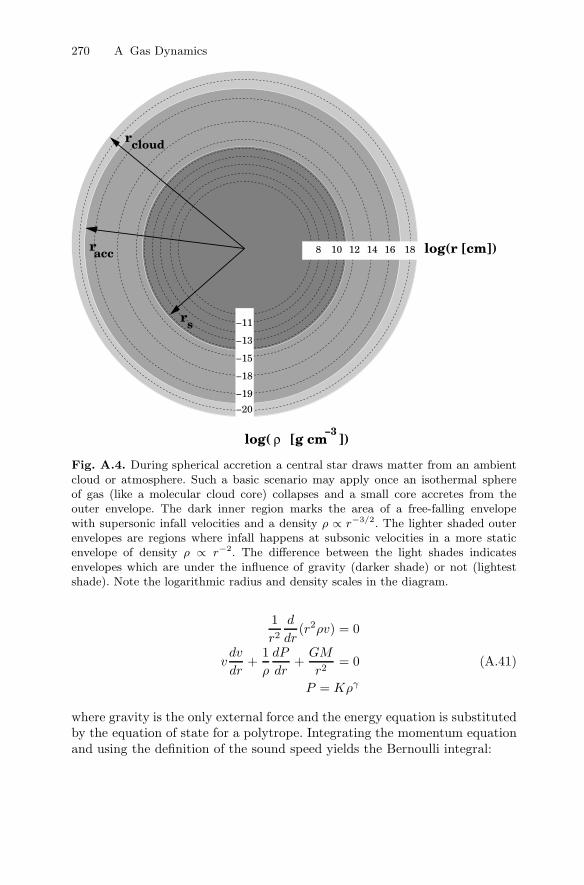
Fig. A.4. During spherical accretion a central star draws matter from an ambientcloud or atmosphere. Such a basic scenario may apply once an isothermal sphereof gas (like a molecular cloud core) collapses and a small core accretes from theouter envelope. The dark inner region marks the area of a free-falling envelopewith supersonic infall velocities and a density ρ ∝ r−3/2. The lighter shaded outerenvelopes are regions where infall happens at subsonic velocities in a more staticenvelope of density ρ ∝ r−2. The difference between the light shades indicatesenvelopes which are under the influence of gravity (darker shade) or not (lightestshade). Note the logarithmic radius and density scales in the diagram.

1r2

d

dr(r2ρv) = 0

vdv

dr+

1ρ

dP

dr+

GM

r2= 0 (A.41)

P = Kργ

where gravity is the only external force and the energy equation is substitutedby the equation of state for a polytrope. Integrating the momentum equationand using the definition of the sound speed yields the Bernoulli integral:

A.11 Rotation 271

v2

2+

c2s

γ − 1− GM

r= const. (A.42)

Note that this integration is not mathematically valid for γ = 1, the strictisothermal case. Here the integral has to be evaluated logarithmically. Thishowever does not change the physical content of this integral. There is acritical radius within which the gas flow changes from subsonic to supersonic.This is called the sonic radius [264]:

rs =GM

2c2s(rs)

7.5 × 1013

(T (rs)

[104 K]

)−1(M

[M]

)cm (A.43)

For a protostellar core accreting from a 1 M molecular cloud of 10 K tem-perature this radius would be about 7.5× 1010 cm. Below this radius the gasflow becomes increasingly supersonic and effectively free falling. In terms ofa cloud size of 0.1 pc this means that throughout most of the cloud the gasflow will stay subsonic.

The above equations also allow one to derive an accretion rate from condi-tions at the outer boundary of a molecular cloud [264]. This derivation leadsto:

M 1.4 × 1011

(M

[M]

)2(ρ(∞)

[10−24g cm−3]

)(cs(∞)

[10 km s−1]

)−3

g s−1 (A.44)

For the case described above and typical values for ρ(∞) (10−20 g cm−3) andcs(∞) (0.35 km s−1) this yields an accretion rate of the order of 10−7 M yr−1.Note that in the spherical Bondi case the mass accretion rate depends on M2,whereas for disk accretion (see Chap. 7) it is independent of mass.

A.11 Rotation

Rotation has a profound effect on the stability of an ideal gas cloud. Sinceangular momentum remains conserved, any cloud will rotate faster as it col-lapses and centrifugal forces will eventually balance and even surpass gravityeverywhere. Thus the cloud’s certain fate is dispersion into the interstellarmedium. To investigate the equation of motion of particles in a uniformlyrotating cloud it is convenient to operate in a frame moving with the rotatingcloud implying that the initial velocity of the cloud element is zero. The op-erator for the rate of change in the inertial frame to the change as measuredin the rotating frame is:

DuDt

=(

dudt

+ Ω× r)

(A.45)

272 A Gas Dynamics

where u = urot + Ω× r and Ω is the angular velocity of the rotating frame.Applying rotation to the equation of hydrostatic equilibrium one finds for theequation of motion in the rotating frame:

dvdt

= −1ρ∇P −∇φ − 2Ω× v − Ω× (Ω × r) (A.46)

where Ω is the angular velocity of the rotating frame. Most of the terms in theequation are familiar. There are two new terms due to rotation: the Coriolisacceleration term (second from right) and the centrifugal acceleration term. Todescribe the equilibrium configuration of rotating clouds only the centrifugalterm is of interest since ideally in equilibrium u is equal to zero.

In a slowly and uniformly rotating cloud centrifugal forces will break thespherical symmetry of the cloud and the system may find another stableequilibrium configuration. Using spherical polar coordinates the rotation axispoints along the unit vector in the polar direction. The centrifugal accelerationcan then be expressed as the gradient of a potential; that is:

Ω× Ω× r = −∇(12Ω2r2 sin2 θ) (A.47)

and (A.46) can finally be rewritten as:

∇P = −ρ∇(φ − 12Ω2r2 sin2 θ) (A.48)

Chandrasekhar in 1969 [161] realized that the potential on the right-handside satisfies Poisson’s equation. The final Chandrasekhar–Milne expansion fora distorted star is shown in (A.21). For a given radius at the poles (θ = 0, π)the effective potential is simply the gravitational potential; at the equator(θ = π/2) the centrifugal pull is maximal. Remarkable in (A.48) is the factthat the gravitational potential is reduced by the effect of rotation with thesquare of the angular velocity. For typical molecular cloud average densitiesof 10−20 g cm−3 this means that rotational velocities cannot exceed 10−14 cms−1 by much because then the centrifugal force would outweigh gravity.

The case of the slowly and uniformly rotating cloud considered above rep-resents a solid body motion and may not be directly applicable for molecularclouds. Although the case is therefore a bit academic it still exhibits valid in-sights into the effects of cloud rotation. For the case of gravitational collapseof a molecular cloud, angular velocity has to increase as radius decreases. Thecollapse soon will come to a halt as centrifugal forces surpass gravity. Oneway out of this problem is to transport angular momentum out of the system;another is to break the cloud up into fragments, thus distributing some ofthe momentum. In the simple ideal gas cloud configuration considered this isnot possible unless one reconsiders the assumptions that all particles in thecloud are neutral, collisions between particles are purely elastic and no exter-nal fields are involved. The final sections of Chap. 4 and much of Chap. 5 dealwith this problem.

A.13 Thermal Ionization 273

A.12 Ionized Matter

So far the description of gaseous matter has been based entirely on the as-sumption that there are no fractions of ion species and no interactions stem-ming from the fact that matter elements carry a net charge. In reality, thereis hardly such an entity as a gas cloud that consists entirely of neutral parti-cles. Within the Galaxy there is always the interstellar radiation field as wellas Cosmic Rays. In contrast, the intergalactic medium outside the Galaxy isconsidered to be entirely ionized. Thus, gas and molecular clouds within theGalaxy always carry non-zero ionization fractions. As long as clouds remainelectrically neutral over a large physical extent they can stably exist as aplasma cloud. Clouds have to be neutral as a whole, since electrostatic forcesattract opposite charges and neutralize the cloud. Gaseous matter thus con-sists not only of neutral atoms and molecules but also of ions, radicals and freeelectrons. Similarly important with respect to the distribution of these ionsare the corresponding electrons. The properties of a plasma are determinedby the sum of the properties of its constituents. The density of a plasma isgiven by:

ρ =∑

k=i,e,n

ρk =∑

k=i,e,n

nkmk (A.49)

where the subscripts i, e and n refer to various ions, all electrons, and variousneutral particles. The kinetic energy of the plasma in thermal equilibrium is:

32kT =

12

∑k=i,e,n

mk < v2k > (A.50)

where vk is the mean square velocity of each constituent. Collisions betweendifferent particles ensure that the mean energies of all particles are the same.The velocity distribution f(v) of each plasma constituent is Maxwellian:

f(v)dv = 4π

[(m

2πkT

])3/2

v2e−mv2/kT dv (A.51)

The peak of this distribution is then vpeak =√

2kTm .

A.13 Thermal Ionization

Section A.4 dealt with thermal excitation and (A.14) expressed the distribu-tion of excited states relative to the ground state. If collisions transfer energiesE larger than a specific ionization energy χion the atom will become ionized.The electrons then have a kinetic energy Ee = E − χion. The Saha equationspecifies the fraction of ionized atoms with respect to neutral atoms:

274 A Gas Dynamics

ni

nn=

Gi

Gn

2ne

(2πmekT )3/2

h3e−χion/kT (A.52)

where Gi

Gois the partition function ratio between ionized and neutral atoms.

This equation was first developed by M. N. Saha in 1920. The important issuein (A.52) is that the ionization fraction is a function of temperature only,as all other ingredients are ionization properties of the gas. The necessarypartition functions for all major elements of interest are tabulated [314] viathe temperature measure Θ = 5040

T [K] . In the case that all atoms are at leastpartially ionized, (A.52) is still valid to determine the fraction between twoionization states. Implicitly, there is also a dependence on electron pressurePe = nekT , and thus (A.52) can be expressed numerically as:

ni

nn=

Φ(T )Pe

,

where Φ(T ) = 1.2020× 109 Gi

GnT 5/210−Θχion (A.53)

Today’s spectral analysis is routine and uses tabulated values for partitionfunctions and ionization potentials [314].

To thermally ionize a gas cloud requires high collision rates, such as thosein stellar atmospheres at temperatures ranging from 3,500 to 40,000 K. Forexample, at an electron pressure of 10 Pa in the atmospheres of main sequencestars, matter is completely ionized at temperatures above 10,000 K and theelectron pressure is of the order of the gas pressure since np ∼ ne. Note that therelation between gas pressure and electron pressure depends on the metallicityof the gas cloud. At low temperatures most electrons come from elements withfirst ionization potentials of less than 10 eV. Applied to a cold gas cloud ofless than 100 K it is clear that thermal ionization hardly contributes to theionization fraction and electron pressure.

A.14 Ionization Balance

At the low temperatures of molecular clouds, the effect of thermal ionizationis small compared with photoionization. Gaseous matter exposed to externaland internal radiation fields is heated. The temperature in a static ionizedgas cloud is determined by the balance between heating through photoioniza-tion events and cooling through successive recombination. Clouds lose energythrough radiation which has to be accounted for in the energy balance. Ab-sorption of the radiation field produces a population of free electrons whichare rapidly thermalized. The mean energy of a photoelectron does not dependon the strength of the incident radiation field but on its shape. For example,if the radiation field does not provide photons of energies 13.6 eV (912 A) andhigher, then a hydrogen cloud is unlikely to be effectively ionized. The rate of

A.14 Ionization Balance 275

creation of photoelectrons critically depends on the absolute strength of thefield and the ability of the gas to recombine. To establish the energy balanceof a gas cloud and its ambient radiation field one has to consider the heatingrate through photoionization Rphoto against cooling through recombinationRre, free–free (bremsstrahlung) radiation Rff and collisionally excited lineradiation Rcol. Usually, an effective heating rate Reff is defined as:

Reff = Rphoto − Rre = Rff + Rcol (A.54)

where it should be noted that Rphoto and Rre depend on the number densitiesof electrons and ions, and, as a valid approximation, elements heavier thanHe may be omitted in these rates.

B

Magnetic Fields and Plasmas

Some aspects concerning the modern treatment of stellar magnetic fields arerevisited here in greater detail. Magnetic fields and their interactions withmatter are very crucial elements in the study of the formation and early evo-lution of stars. This appendix highlights the interaction of magnetic fields ina much more fundamental way than presented in the previous chapters andmuch of what is presented has a wide range of applications, likely much be-yond the scope of this book. The material is collected from a wide variety ofpublications, though only in rare cases will references be given. The appendixmakes heavy use of material presented in the books by F. H. Shu: Gas Dynam-ics, Vol. II [781], and E. Priest and T. Forbes: Magnetic Reconnection [701].In this respect it should be noted that the following is merely to supportthe reader to understand certain subtleties in this book. For a full recourseto magnetism and its interaction with matter the reader should consult theprimary literature.

B.1 Magnetohydrodynamics

The study of the global properties of plasmas in a magnetic fields is calledMHD. The most basic equations are Maxwell’s equations (after J. Maxwell1872):

∇ · E = 4πqe (B.1)

∇ × E = −1c

∂B∂ t

(B.2)

∇ · B = 0 (B.3)

∇ × B =4π

cj +

1c

∂E∂ t

, (B.4)

278 B Magnetic Fields and Plasmas

which, by ignoring the displacement current 1c

∂E∂ t , contain the laws of the

conservation of charge (B.1), Faraday’s equation (B.2), Gauss’s law (B.3),and Ampere’s law (B.4), respectively. In order to include magnetic and electricfields in fluid mechanics one has to re-formulate some of the conservation lawsas stated in Sect. A.6. In this respect, mass conservation remains unchangedbut all the other equations have to be modified.

The momentum equation of a MHD fluid element then reads:

ρ∂v∂t

+ ρ(v · ∇)v = −∇P +1c(j × B) + ∇S + Fg (B.5)

This equation shows a few important modifications with respect to the stress-free Euler equation (A.24). For the magnetic field it includes the magneticforce in the form of the vector product of the current density J and themagnetic field strength B and, besides identifying the gravitational force Fg

as external force, considers the stress term ∇S. By invoking Ampere’s law onecan see that this magnetic force consists of a magnetic pressure force and amagnetic tension force:

1cj× B = − 1

8π∇B2 +

14π

(B · ∇)B (B.6)

MHD fluids are usually not stress-free and instead of Equation A.24 onehas to consider the general Navier–Stokes equation for a viscous fluid element.Magnetic fields under these conditions also permeate into the stress tensor,which, depending on the field strength and plasma conditions is an expressionof considerable complexity. For a magnetic field strength of 50 G, a plasmadensity of 3×109 cm−3 and a proton temperature of 2.5×106 K, for example,the stress tensor S can be expressed in component form as [119, 409]:

Sij = 3ηv

(δij

3− BiBj

B2

)(B ·B∇v

B2− ∇v

3

)(B.7)

Here ηv = 10−16 T 5/2 g cm−1 s−1 is a viscosity coefficient and δij is theKronecker delta function.

Similarly complex is the Ansatz for the energy equation (A.28), which nowreads like:

∂U

∂t+ ∇[(U + P )v] = ∇(κc∇T) + (ηej) · j + Qν − Qrad (B.8)

Again the left-hand side is the change in specific energy plus the work per-formed by the system either by expansion or contraction. The right-hand sidein (A.28) was kept rather general. In the MHD case of (B.8) these termsare now further identified. In this respect, Qrad = ∇Frad is radiative energyloss, Qν is heating by viscous dissipation with tight relation to the stress ten-sor. The first term on the right-hand side is to describe thermal conductivitycharacterized by the thermal conductivity tensor κc and the temperature Tat each location. The second term on the right is the magnetic energy.

B.1 Magnetohydrodynamics 279

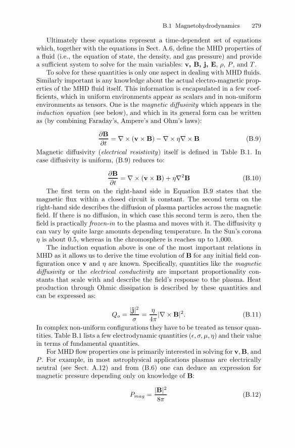
Ultimately these equations represent a time-dependent set of equationswhich, together with the equations in Sect. A.6, define the MHD properties ofa fluid (i.e., the equation of state, the density, and gas pressure) and providea sufficient system to solve for the main variables: v, B, j, E, ρ, P , and T .

To solve for these quantities is only one aspect in dealing with MHD fluids.Similarly important is any knowledge about the actual electro-magnetic prop-erties of the MHD fluid itself. This information is encapsulated in a few coef-ficients, which in uniform environments appear as scalars and in non-uniformenvironments as tensors. One is the magnetic diffusivity which appears in theinduction equation (see below), and which in its general form can be writtenas (by combining Faraday’s, Ampere’s and Ohm’s laws):

∂B∂t

= ∇× (v × B) −∇× η∇× B (B.9)

Magnetic diffusivity (electrical resistivity) itself is defined in Table B.1. Incase diffusivity is uniform, (B.9) reduces to:

∂B∂t

= ∇× (v × B) + η∇2B (B.10)

The first term on the right-hand side in Equation B.9 states that themagnetic flux within a closed circuit is constant. The second term on theright-hand side describes the diffusion of plasma particles across the magneticfield. If there is no diffusion, in which case this second term is zero, then thefield is practically frozen-in to the plasma and moves with it. The diffusivity ηcan vary by quite large amounts depending temperature. In the Sun’s coronaη is about 0.5, whereas in the chromosphere is reaches up to 1,000.

The induction equation above is one of the most important relations inMHD as it allows us to derive the time evolution of B for any initial field con-figuration once v and η are known. Specifically, quantities like the magneticdiffusivity or the electrical conductivity are important proportionality con-stants that scale with and describe the field’s response to the plasma. Heatproduction through Ohmic dissipation is described by these quantities andcan be expressed as:

Qo =|j|2σ

=η

4π|∇ × B|2. (B.11)

In complex non-uniform configurations they have to be treated as tensor quan-tities. Table B.1 lists a few electrodynamic quantities (ε, σ, µ, η) and their valuein terms of fundamental quantities.

For MHD flow properties one is primarily interested in solving for v,B, andP . For example, in most astrophysical applications plasmas are electricallyneutral (see Sect. A.12) and from (B.6) one can deduce an expression formagnetic pressure depending only on knowledge of B:

Pmag =|B|28π

(B.12)


Table B.1. Characterization of MHD plasmas

Symbol Name Form Expression

ε dielectric constant scalar 1 + (πρc2/B2)σ electric conductivity tensor nee

2/meνc

ω2pe/4πνc

µ magnetic permeability scalar (1 + (4πρE⊥/B2))−1

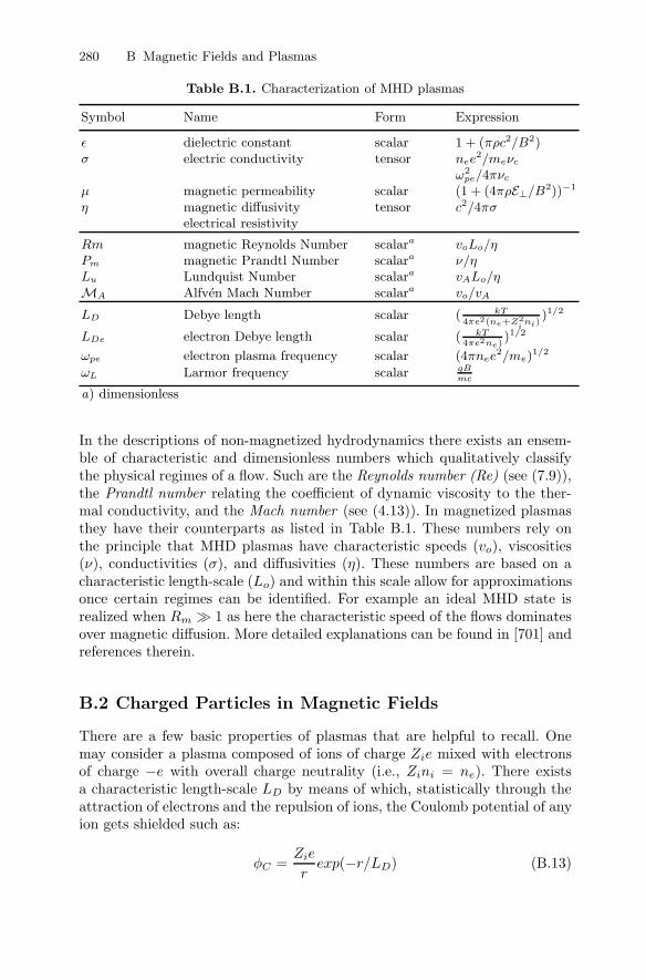
η magnetic diffusivity tensor c2/4πσelectrical resistivity

Rm magnetic Reynolds Number scalara voLo/ηPm magnetic Prandtl Number scalara ν/ηLu Lundquist Number scalara vALo/ηMA Alfven Mach Number scalara vo/vA

LD Debye length scalar ( kT4πe2(ne+Z2

ini)

)1/2

LDe electron Debye length scalar ( kT4πe2ne)

)1/2

ωpe electron plasma frequency scalar (4πnee2/me)

1/2

ωL Larmor frequency scalar qBmc

a) dimensionless

In the descriptions of non-magnetized hydrodynamics there exists an ensem-ble of characteristic and dimensionless numbers which qualitatively classifythe physical regimes of a flow. Such are the Reynolds number (Re) (see (7.9)),the Prandtl number relating the coefficient of dynamic viscosity to the ther-mal conductivity, and the Mach number (see (4.13)). In magnetized plasmasthey have their counterparts as listed in Table B.1. These numbers rely onthe principle that MHD plasmas have characteristic speeds (vo), viscosities(ν), conductivities (σ), and diffusivities (η). These numbers are based on acharacteristic length-scale (Lo) and within this scale allow for approximationsonce certain regimes can be identified. For example an ideal MHD state isrealized when Rm 1 as here the characteristic speed of the flows dominatesover magnetic diffusion. More detailed explanations can be found in [701] andreferences therein.

B.2 Charged Particles in Magnetic Fields

There are a few basic properties of plasmas that are helpful to recall. Onemay consider a plasma composed of ions of charge Zie mixed with electronsof charge −e with overall charge neutrality (i.e., Zini = ne). There existsa characteristic length-scale LD by means of which, statistically through theattraction of electrons and the repulsion of ions, the Coulomb potential of anyion gets shielded such as:

φC =Zie

rexp(−r/LD) (B.13)

B.3 Bulk and Drift Motions 281

where LD is the Debye length defined in Table B.1. It is sometimes usefulto decouple the electron contribution and define a separate electron Debyelength, which allows one to deduce a characteristic electron plasma frequencyωpe. In other words, the electronic portion of the plasma can be described bythe dynamics of a harmonic oscillator with a natural frequency of ωpe.

The presence of magnetic fields in gas clouds with substantial ionizationfractions has a profound effect on the dynamics of the plasma. The gas orplasma pressure is then expressed as the average momentum of gas particlesP = Nm < v2

ijk >, where vijk and is now treated as a tensor. In the simpleideal gas case this pressure tensor is diagonal and since collisions dominate, alldirections are equal and < v2

ijk >= v2. In the case of a non-negligible magneticpressure one needs to distinguish between pressure components across andalong magnetic field lines. The magnetic field thus directs the charged particleswithin the three orthogonal spatial coordinates (xi, xj , xk) and the pressuretensor possesses off-diagonal terms.

The motions of individual particles with charge q and mass m in a vectormagnetic field B are described by the force:

F =dpdt

= qE +q

cv × B (B.14)

where p is the momentum vector and v the velocity vector of the particle.Called the Lorentz-force it was first formulated by H. A. Lorentz in 1892.The particle then gyrates in a clockwise path when q is a negative charge,and counterclockwise when it is a positive charge. The gyro-radius in thenon-relativistic case (also called Larmor radius) is given by:

rL =mcv⊥qB

=v⊥ωL

(B.15)

where v⊥ is the velocity perpendicular (⊥) to the field and ω the gyro-frequency. The thermal energy per unit volume associated with the gyro-motion about the field lines (ρE⊥) is given by the integral over a velocitydistribution function (see Sect. A.12) and a sum over all particles as:

ρE⊥ =∑ ∫

12mv2

⊥fd3v (B.16)

B.3 Bulk and Drift Motions

For the bulk of particles the average motion in the presence of uniform electricand magnetic fields is perpendicular to both fields, and for weak electric fieldsimplies an average velocity due to an E× B drift of:

vbulk =cE× B

B2(B.17)


In general, drift currents are the sources of many astrophysical magnetic fields.Note that the resulting bulk motion is always perpendicular to the force. Thefollowing extends the above consideration to the inclusion of external forcefields, in this case gravitational force. The equation of motion then reads:

mv = qE +q

cv × B + mg (B.18)

Under the simplified situation where g and E are perpendicular to B – some-thing that is realized in many astrophysical cases and which many times isreferred to as crossed field cases – one can rewrite (B.18) such that:

mv =q

c

(v − vbulk − mc

q

g × BB2

)(B.19)

The g × B drift is well known from the near-Earth environment as it causescharged particles in the radiation belts to circulate in an azimuthal direction asas well as to shuttle back and forth between the Earth’s magnetic poles [781].Besides the normal gyro motion, the crossed field case then provides severaldrift motions including the electric (B.17) and gravitational drift (B.19), andthe polarization drift in time-dependent fields.

Drifts and drags are also present in partially ionized media such as molec-ular clouds or near neutral winds. In this case a relative drift arises betweenthe neutral and ionized particle species of the medium simply due to the factthat ions feel electromagnetic forces directly, whereas neutral particles have toengage in collisions with the ions. Neutral matter in general is not affected bythe presence of magnetic fields. This relative drag is called ambipolar diffusion(see Sect. 4.3.4). The Lorentz force felt by the charged particles in a magneticfield within a unit volume reads:

FL =14π

(∇× B) × B (B.20)

Since this force is not felt by neutrals, ions will drift with a different meanvelocity. Resisting this drift will result in a frictional drag force created bymutual collisions. The drag force on neutral species by ion species can beexpressed as:

Fd = γdnnnimnmi(vi − vn) (B.21)

where γd is the drag coefficient:

γd =< uσ >

mn + mi(B.22)

and where n, m, and v (index n for neutral, i for ionized) are number density,mass, and mean velocity of neutral (n) and ionized (i) species. For simplicityit was assumed that the mass densities of these species can be expressed byρ = nm. The term ni < uσ > is the rate of collisions of ions with anyneutral of comparable size. The bracketed expression is a mean of the elastic

B.4 MHD Waves 283

scattering cross section for neutral-ion collisions and the relative velocity ofthe ions in the rest frame of the neutrals. The ambipolar drift velocity canthen be determined by:

wD = vi − vn =1

4πγdnnnimnmi(∇× B) × B (B.23)

which in the case of magnetic uniformity is equivalent to the expression givenin (B.17). The sign of the drift depends on a definition of the drag direction(i.e., whether it is the drag on the neutral by the ions or vice versa).

B.4 MHD Waves

Another important application of MHD is the propagation of waves throughmagnetized plasma. The subject of MHD waves is considerably more com-plex than in ordinary hydrodynamics and, therefore, most treatments areperformed numerically. However, the propagation of shocks and disturbancesin magnetized plasmas has many astrophysical applications specifically in stel-lar formation research and a summary of a few main properties is warranted.

A simple case is an ideal gas in static, uniform equilibrium with velocityvo = 0, density ρ = ρo, pressure P = Po, and a constant uniform magneticfield |Bo| = constant. By introducing a small perturbation these conditionsthen read:

ρ = ρo(1 + ε), v = v1, P = Po(1 + ψ), B = Bo(n + n′) (B.24)

The standard MHD equations under these conditions reduce to a set of equa-tions describing the response of the perturbations to the magnetic field:

∂ε

∂t+ ∇v1 = 0

∂v1

∂t+

Po

ρo∇ψ − B2

o

4π(∇× n′) × n = 0

∂n′

∂t+ ∇× (n× v1) = 0

∂ψ

∂t− γ

∂ε

∂t= 0

(B.25)

For the last relation the equation of state for ideal gas (see Sect. A.2) wasapplied. It thus describes the propagation of an adiabatic perturbation wherethe coefficient γ is the adiabatic index. Combining these equations and ap-plying the definitions to the speed of sound and the Alfven speed given in


Sect. A.8 leads to a second-order differential equation for the velocity of theperturbation with a solution of the form:

v1 = exp[i(ω1t − k · x)], (B.26)

where ω1 is the perturbation propagation frequency and k the momentumvector plane of propagation. By splitting the wave equation into coordinatecomponents one can identify various wave modes with respect to the plane ofpropagation and the magnetic field.

One of these modes is a transverse wave with wavefronts perpendicular tok = kez and n = ex cos φ + ey cos φ, i.e., with v1 = (vx = 0, vy = 0, vz):

ω2 − k2v2A cos2 φ = 0 (B.27)

This wave mode is generally referred to as an Alfven wave. In the case ofφ = 0 the wave speed is equal to the Alfven velocity (see Sect. A.8). In the caseof φ = 0 the wavefronts may be considered to be inclined with respect to theunperturbed magnetic field. Thus, Alfven waves always travel at Alfven speedand vA cos φ merely represents the projection with respect to the magneticfield vector. Other modes under these conditions are identified as slow andfast MHD waves. It should also be noted that this simple picture, thoughapproximately valid for many applications, is based on uniform and stress-free environments and, thus, in detail the treatment of MHD waves is highlycomplex.

B.5 Magnetic Reconnection

In many astrophysical situations it appears that one way or another the topol-ogy of the present magnetic field configuration is not conserved and subjectto what is called magnetic reconnection. Such events have been mentioned inconnection with molecular clouds for star-disk field configurations and as theprime underlying mechanism for stellar flaring activity (see Chap. 7).

Most treatments of magnetic reconnection are two dimensional and theirdescriptions involve many aspects, some of which will be described here. Bydefinition, reconnection cannot take place under ideal MHD conditions, be-cause it needs resistivity in the medium. Such resistivity is usually providedthough collisions. However, nature proves a bit more resilient towards thesearguments as reconnection events happen in the terrestrial magnetospherewithin almost collisionless environments. In order to classify reconnectionprocesses, it is thus necessary to determine the reconnection rate in variousconfigurations even if they contain collisionless plasmas.

There are quite a number of reconnection processes and not all are ofinterest to stellar evolution research. Some of the basic ideas on the effect ofmagnetic reconnection were described by P. A. Sweet 1956 and E. Parker in1957 [825, 664, 665]. Central to this are magnetic field configurations that

B.5 Magnetic Reconnection 285

Null (X) point

2L x

2Ly

Inflow with v

Ou

tflo

w w

ith

v x

y

−B

B

Null sheet

High pressure Medium pressure Low pressure

B

−B

B’

−B’

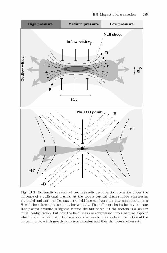
Fig. B.1. Schematic drawing of two magnetic reconnection scenarios under theinfluence of a collisional plasma. At the tops a vertical plasma inflow compressesa parallel and anti-parallel magnetic field line configuration into annihilation in aB = 0 sheet forcing plasma out horizontally. The different shades loosely indicatethat plasma pressure is highest around the null sheet. At the bottom is a similarinitial configuration, but now the field lines are compressed into a neutral X-pointwhich in comparison with the scenario above results in a significant reduction of thediffusion area, which greatly enhances diffusion and thus the reconnection rate.


feature parallel and antiparallel field lines separated by a B = 0 surface,and an incompressible fluid where the total pressure remains constant. Ohmicdissipation near this null surface causes field annihilation. In 2-D treatments,this location is sometimes also called null sheet. Changes in the gravitationalpotential are regarded to be negligible within a characteristic volume Vo =LxLyLz. For this simple configuration (see also the top diagram in Fig. B.1),the reconnection speeds of the plasma can be expressed in terms of the Alfvenspeed. Essentially, the plasma pushes the field lines into the null sheet fromboth vertical directions, squeezing plasma out in the horizontal direction. Theenergy dissipation rate per unit volume (see (B.11)) is then given by:

Qo =η

4π

(B

Ly

)2

. (B.28)

This allows us to calculate the heat produced within Vo, which should be equalto the annihilation energy pressed into the region; that is:

ηB2

4πLy=

B2

8πLxLzvy (B.29)

where vy represents the reconnection speed. It is also the plasma speed in they-direction with which the plasma flow is pushing the field lines into the nullsheet. Using the expression for the magnetic Reynolds number in Table B.1it is clear that the relation between the reconnection speed and the Alfvenvelocity is a function of the magnetic Reynolds number of the horizontaloutflow Rm. The reconnection rate Me in this case yields:

Me =vy

vA= 2R−1/2

m (B.30)

On the other hand, the magnetic Reynolds number in astrophysical plas-mas is usually a very large number. For a collisional plasma with a strong mag-netic (but weak electric) field, magnetic diffusivity can be written as [800, 751]:

η = 1.05 × 1012T−3/2 lnΛ cm2 s−1 (B.31)

where ln Λ is the Coulomb logarithm [411]. For typical molecular cloud pa-rameters as well as most laboratory applications lnΛ has a value of ∼ 10,and for collisional plasmas in stellar coronae and the Earth’s magnetosphereit is higher than 20 but not more than 35. For most cases it is safe to as-sume that the characteristic velocity of the magnetized plasma is the Alfvenvelocity and, thus, the magnetic Reynolds number can be approximated bythe Lundquist number Lu. Thus, for active regions in the solar corona, wherethe temperature can get beyond 107 K, assuming loop lengths of 107 cm, anapproximate Alfven speed of ∼ 107 cm s−1, η ∼ 7 × 102 cm2 s−1, the Lu

number is about 1011. Above a more active region it can even reach 1014.

B.6 Dynamos 287

From (B.30) it appears that reconnection takes place at a fraction of thedynamical speed of magnetized plasma. In turn this means that magneticdiffusion, with a timescale defined as:

τmd =L2

o

η(B.32)

requires very long timespans. Although in rare cases this may be what hap-pens, it certainly cannot explain the sunspot and flaring activity on the Sun.Similarily, it is not feasible to describe magnetic young stellar activity. How-ever, the Sweet–Parker scenario of field annihilation of a null sheet of limitedsize doesn’t really maximize the possible reconnection rate. In 1963 H. E.Petschek thus proposed a slightly different scenario in which the null sheet iscompressed into an X-point [676] (see bottom of Fig. B.1). Here magnetic dif-fusion is confined to an area around the neutral point, which as a consequenceenhances diffusion rates and allows field annihilation to accelerate. There aretwo novel features about this reconnection geometry. First, it generates amaximum annihilation rate of the form:

Mmaxe =

vy

vA∼ π

8 lnRm(B.33)

where the index e stands for external (i.e., for the inflow which is not near theX-point). Second, it allows the magnetic field to diffuse into the plasma whereit propagates as an MHD wave outward [676]. This generates reconnectionrates between 0.01 and 0.1, leading to much shorter timescales consistentwith observed flaring activity (see Chaps. 7 and 8).

B.6 Dynamos

In the most general sense, the magnetic dynamo theory describes MHD flowswithin stellar bodies that feature differential rotation and convection. It isa common perception among astrophysicists that all stellar magnetic fieldshave their origins one way or another through self-excited magnetic dynamoactivity. This may even be true for the interstellar or galactic field throughsome form of galactic dynamo. Though a complete dynamo theory is relativelycomplicated and not at all in every aspect understood, there are a few basicdynamo functions and relations one should recall when dealing with stellarand proto-stellar dynamos.

Complex motions of a plasma with a weak seed magnetic field can generatestrong magnetic fields on larger scales. One would first attempt a simplifiedapproach and try to solve the MHD problem axisymmetrically. Herein liesthe first big problem: dynamos cannot maintain either a poloidal or a toroidalmagnetic field against Ohmic dissipation. As a consequence, exact axisymmet-ric dynamos cannot be realized. This phenomenon is also known as Cowling’s


theorem after T. G. Cowling, formulated in 1965. In other words, the induc-tion equation (B.10) does not allow for axisymmetric fluid motions that yieldnon-decaying and, similarily, axisymmetric configurations for the B-field. Aquite comprehensible illustration of this effect can be found in [781]. Observedphenomena in the Sun (i.e., sunspots, flares and prominences) indicate insteadthat magnetic reconnection is required [701]. It should also be realized thatthe dynamo effect does not generate magnetic fields but amplifies existingones. The following is an attempt to outline some of the groundwork for therealization of MHD dynamos.

Cowlings’s theorem mandates that in order to maintain a seed magneticfield one needs to offset Ohmic dissipation. In addition, in order to get thedynamo going, a cycle has to build up which converts toroidal fields intopoloidal ones and regenerates toroidal fields from converted poloidal ones. Themechanisms proposed include radial convection, magnetic instabilities suchas the magnetostatic Parker Instability and various levels of turbulence. Thecurrent standard theory for Sun-like stars features various modifications of theso called α − Ω dynamo, a concept that took shape in the mid-1950s [663].In simple terms, this may be described by a uniform magnetic field beingdeformed locally into Ω-shaped loops through cyclonic turbulence-generatingeddies which have a cyclonic velocity α. The theoretical basis to describethe toroidal field is the induction equation. By neglecting other forces thisequation can be simplistically formulated as [663, 484]:

∂B∂t

= η∇2B − α∇× B (B.34)

where α is defined as:

αB = u × b (B.35)

Where u and b are the velocity and induction field of the generated stand-ing MHD wave solution. Within a characteristic length scale Lo the charac-teristic dynamo period is tied to the eddy diffusivity ηed as:

τdy =L2

o

4ηed(B.36)

Eddy diffusivity characterizes the stability of the eddies creating the Ω-loops. For an azimuthal field flux written as Φ = LoB the dynamical periodcan be expressed in terms of B and Φ. For the solar period of 22 yr this has theconsequence that as long as ηed is not suppressed by more than 1/B2, such along period can be maintained in the presence of strong azimuthal fields [667].

Modern versions of this dynamo recognize the fact that helioseismologicaldata suggest that the Solar dynamo operates in only a small layer within theSun’s interior (see [667, 162, 550] and references therein). This layer is locatedat about 0.7 R from the center between the boundary of the convectiveouter zone and the radiative core and has a thickness of less than 3 percent

B.6 Dynamos 289

−z

z

z

x

δb = − a/ zx δ δb ( x , z , t ), η

2

Convective

Radiative

B = − A/ x

B = − A/ zB ( x , z , t ),

x

z δδδ δ

α − Ω zone

η

δ δ δ δb = B , a= A , a/ z = A/ z

1

η2 δ b/ z = B/ zδ δ δη1

Shear zone −h/2

+h/2

b = − a/ xz δ

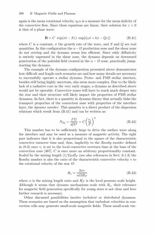
Fig. B.2. (left) Illustration of the α − Ω dynamo effect in the Sun. The inner corerepresents the radiative zone, the outer shell the convective zone. In-between is thethin layer in which the actual dynamo operates. The thick lines with arrows arewound up and surfaced magnetic field lines. (right) A diagram that highlights theseparation of the layer into the α−Ω part below the convective zone and the shearpart above the radiative zone together with the corresponding field specifications(see dynamo equation in the text). Highlighted at z = 0 are the necessary boundaryconditions. The configuration described here is called the interface dynamo. Themagnetic diffusivity is η1 in the α − Ω zone, η2 in the shear zone.

of the stellar radius. The vertical shear ∂Ω/∂r is also confined to this layer,meaning there is no significant change of radial velocity between the top andthe bottom of the convection zone. Figure B.2 illustrates schematically theset-up for such an interface dynamo. One configuration of such a dynamo wasproposed by Parker in 1993 and is illustrated in Fig. B.2. The actual dynamoequations according to the specifications in Fig. B.2 read [667]:

[∂

∂t− η1

(∂2

∂x2+

∂2

∂z2

)]B = 0 (B.37)[

∂

∂t− η1

(∂2

∂x2+

∂2

∂z2

)]A = αB (B.38)[

∂

∂t− η2

(∂2

∂x2+

∂2

∂z2

)]b = G

∂a

∂x(B.39)[

∂

∂t− η2

(∂2

∂x2+

∂2

∂z2

)]a = 0 (B.40)

Where A and a are the azimuthal vector potentials describing the poloidalfield for z > 0 and z < 0, respectively; G is the uniform shear dvy/dz; α once


again is the mean rotational velocity, η1α is a measure for the mean helicity ofthe convective flow. Since these equations are linear, their solution for z > 0is that of a plane wave:

B = C exp(σt − Sz) exp[i(ωt + kx − Qz)] (B.41)

where C is a constant, σ the growth rate of the wave, and S and Q are realquantities. In this configuration the α−Ω production zone and the shear zonedo not overlap and the dynamo seems less efficient. Since eddy diffusivityis entirely supressed in the shear zone, the dynamo depends on downwardpenetration of the poloidal field created in the α − Ω zone, practically jump-starting the dynamo.

The example of the dynamo configuration presented above demonstrateshow difficult and fragile such scenarios are and how many details are necessaryto successfully operate a stellar dynamo. Proto- and PMS stellar interiors,besides still being highly uncertain, also seem more complex. Due to the likelylack of a radiative core in the very early stages, a dynamo as described abovewould not be operable. Convective zones will have to reach much deeper intothe star and their structure will likely impact the properties of PMS stellardynamos. In fact, there is a quantity in dynamo theory that actually links thetransport properties of the convection zone with properties of the interfacelayer, the dynamo number . This quantity is a direct product of the dispersionrelations which result from (B.41) and can be written as:

Ndy =ΓG

η21k

3= C

(τc

P

)2

(B.42)

This number has to be sufficiently large to drive the surface wave alongthe interface and may be used as a measure of magnetic activity. The rightpart indicates that it is also proportional to the square of the characteristicconvective turnover time and, thus, implicitly to the Rossby number definedin (8.3) once τc is set to the local convective overturn time at the base of theconvection zone [467]. C is once more an arbitrary proportionality constant.Scaled by the mixing length (1/2)αHP (see also references in Sect. 6.1.3) theRossby number is also the ratio of the characteristic convective velocity v tothe rotational velocity of the star Ω:

Ro =2πv

αΩHP(B.43)

where α is the mixing length ratio and HP is the local pressure scale height.Although it seems that dynamo mechanisms scale with Ro, their relevancefor magnetic field generation specifically for young stars is not clear and herefurther research is necessary.

Other discussed possibilities involve turbulent or distributed dynamos.These scenarios are based on the assumption that turbulent velocities in con-vection cells may generate small-scale magnetic fields. These small-scale tur-

B.7 Magnetic Disk Instabilities 291

bulent fields may even co-exist with the dominant α − Ω dynamo at theinterface layer. In stars with deep convective zones, these turbulent fieldscould be the source for large-scale fields. Most of these concepts need furtherdevelopment [213, 490, 755].

B.7 Magnetic Disk Instabilities

The notion to treat protostellar disks as magnetized rotating fluids haschanged the view of angular momentum transport. MHD waves and tur-bulence introduce perturbations in otherwise smooth flows. Central to thetreatment of magnetized rotating fluids are either fluctuations of velocitiesor densities or both. The basic MHD equations to describe such fluctuationsare again the same as introduced above, now applied towards an accretionflow. Conservation laws are used to illustrate how differential rotation in adisk frees magnetic energy to turbulent fluctuations in combination with an-gular momentum transport. Most of the material in this section was takenfrom a recent review on angular momentum transport in accretion disks byS. A. Balbus [47]. Thus, in addition to the standard MHD set of equationsintroduced above, it is useful to introduce cylindrical coordinates (see below)to satisfy the geometrical constraints of the disk and separate the azimuthalcomponent of the momentum equation. This equation then can be written asangular momentum conservation:

∂(ρrvφ)∂t

+ ∇(

ρrvφv − rBφ

4πB +

(P +

B2

8π

)eφ

)= 0 (B.44)

Note that the dissipative term ρv∇v has been ignored as it carries only anegligible amount of angular momentum. It also helps to simplify the energyequation and write it explicitly for contributing terms only and assume thatmatter is polytropic:

∂U

∂t+ ∇Fe = −Qrad (B.45)

where the energy density U is:

U =12ρv2 +

P

γ − 1+ ρΦ +

B2

8π(B.46)

and similarly for the energy flux Fe are:

Fe = v(

12ρv2 +

γP

γ − 1+ ρΦ

)+

B4π

× (v × B) (B.47)

The terms for kinetic, thermal, gravitational, and magnetic components arenow clearly indicated from left to right, respectively. Again, the heating term


Qν has been dropped as it does not contribute enough overall with respect toenergy conservation.

In order to introduce turbulent fluctuations one defines an azimuthal ve-locity perturbation, such as:

u = v − rΩ(r)eφ (B.48)

where Ω(r) is approximated by the underlying rotational velocity profile.Rewriting the energy equation in terms of the perturbed velocity isolatesthe disk stress tensor responsible for wave and turbulent transport:

∂U

∂t+ ∇Fe = −Srφ − Qrad (B.49)

consisting of Reynolds and Maxwell stresses:

Srφ = ρuruφ − BrBφ

4π(B.50)

These stresses directly transport angular momentum and support turbulenceby freeing energy from differential rotation. For protostellar disks Srφ alwayshas to be positive in order to keep the turbulence from dying out.

φ

J

r

k

k

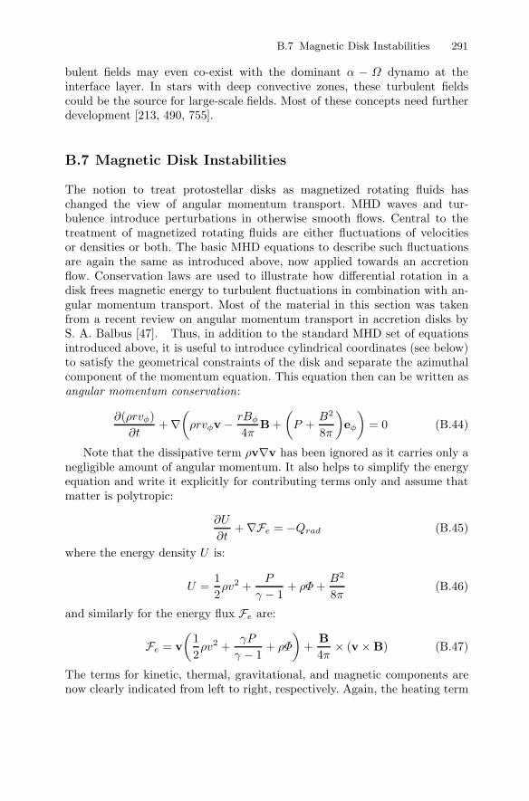
Fig. B.3. In analogy to the MRI effect one may want to consider fluid elementsthat are attached with springs of spring constant k. The fluid array (left) moves ata differential azimuthal velocity (thick black arrows). Since the top elements movefaster than the element immediately following in direction of r, this element feelsa drag that corresponds to the spring constant k. The next element experiencesa similar drag and so on (middle array). Imagine the system springing back toits original differential profile (right array), the shaded area in the middle arraydemonstrates the accumulation of angular momentum that is transported in theradial direction.

B.8 Expressions 293

Reviews on how angular momentum is transported in (proto-) planetarydisks in the absence of a magnetic field can be found in [344, 47]. Some ofthe first calculations on magneto-rotational instability (MRI) can be tracedback to the early 1950s when Chandrasekhar calculated the factors involvedin dissipative Couette flows, though the regime where the gradients of an-gular velocity and specific angular momentum oppose each other were notparticularly pursued [306]. MRI has its roots in the fact that the magneticfield in a differentially rotating fluid acts in a destabilizing way. Figure B.3illustrates the underlying principle in analogy to nearby fluid elements cou-pled with each other by a spring-like force. Due to differential rotation slowerrotating elements experience a drag. At the end the angular momenta of theseslower rotating elements increase at the expense of faster rotating ones. Thespring tension grows with increasing element separation and angular momen-tum transport outward cascades away. In a protostellar systems this analogyroughly describes a very simple fluid system moving in an axisymmetric diskin the presence of a weak magnetic field. In fact, for a fluid element which isdisplaced in the orbital plane by some amount ξ with a spatial dependenceof eikz , the induction equation in the case of frozen-in fields (see above) givesa displacement of the magnetic field of ∂B = ikBξ leading to a magnetictension force, which can be written in the form:

ikB4πρ

∂B = −(kvA)2ξ (B.51)

This equation has the form of the equation of motion for a spring-like force.The result is a linear displacement with a spring constant (kvA)2.

B.8 Expressions

In most astrophysical applications either cylindrical (r, φ, z) or spherical(r, θ, φ) polar coordinates are adopted according to the geometrical constraintsof the MHD fluid. The following most common expressions involving the po-tential A and the field B are spelled out in component form for the twocoordinate systems. The unit vectors for the cylindrical case are er, eφ andez, whereas for the spherical case they are er, eθ and eφ.


Cylindrical polar coordinates:

∇A =∂A

∂rer +

1r

∂A

∂φeφ +

∂A

∂zez

∇ · B =1r

∂

∂r(rBr) +

1r

∂Bφ

∂φ+

∂Bz

∂z

∇× B =(

1r

∂Bz

∂φ− ∂Bφ

∂z

)er +

(∂Br

∂z− ∂Bz

∂r

)eφ +

(1r

∂

∂r(rBφ) − 1

r

∂Br

∂φ

)ez

∇2A =1r

∂

∂r

(r∂A

∂r

)+

1r2

∂2A

∂φ2+

∂2A

∂z2(B.52)

(B · ∇)B =(

Br∂Br

∂r+

Bφ

r

∂Br

∂φ−

B2φ

r+ Bz

∂Br

∂z

)er

+(

Br

r

∂

∂r(rBφ) +

Bφ

r

∂Bφ

∂φ+ Bz

∂Bφ

∂z

)eφ

+(

Bz∂Bz

∂z+ Br

Bz

∂r+

Bφ

r

∂Bz

∂φ

)ez

Spherical polar coordinates:

∇A =∂A

∂rer +

1r

∂A

∂θeθ +

1r sin θ

∂A

∂φeφ

∇ · B =1r2

∂

∂r(r2Br) +

1r sin θ

∂

∂θ(sin θBθ) +

1r sin θ

∂Bφ

∂φ

∇× B =1

r sin θ

(∂

∂θ(sin θBφ) − ∂Bθ

∂φ

)er +

(1

r sin θ

∂Br

∂φ− 1

r

∂

∂r(rBφ)

)eθ

+(

1r

∂

∂r(rBθ) −

1r

∂Br

∂θ

)eφ

∇2A =1r2

∂

∂r

(r2 ∂A

∂r

)+

1r sin θ

∂

∂θ

(sin θ

∂A

∂θ

)+

1r2 sin2 θ

∂2A

∂φ2

(B · ∇)B =(

Br∂Br

∂r+

Bθ

r

Br

∂θ−

B2θ + B2

φ

r+

Bφ

r sin θ

∂Br

∂φ

)er (B.53)

+(

BrBθ

∂r+

Bθ

r

Bθ

∂θ+

BrBφ

r+

Bφ

r sin θ

(∂Bθ

∂φ− cos θBφ

))eθ

+(

BrBφ

∂r+

BrBφ

r+

Bφ

r sin θ

∂Bφ

∂φ+

Bφ

r sin θ

∂

∂θ(Bφ sin θ)

)eφ

C

Radiative Interactions with Matter

This appendix describes the basic radiative processes that have to be con-sidered when radiation interacts with gas clouds, atmospheres and dust. Itcontains a few useful relations which are specifically of interest for the calcu-lation of opacities. The treatment of radiative transport requires all scattering,absorption, and emission processes to be accounted for.

Stellar formation is characterized by episodes of variable radiative proper-ties and the interaction of radiation with various matter and plasma states.Radiative processes are key ingredients to making stars and as such are theonly source of information to diagnose these processes. The following sectionsoutline the basic physics [732, 834] relevant to model calculations and obser-vational diagnostics. Specific emphasis is given to expressions of the r relevantradiative coefficients.

Intensity can simply be defined as:

Iν =dE

dt dΩ dA dν, (C.1)

which is the radiated energy dE per unit time dt, unit angle dΩ, unit areadA, and frequency dν. The general equation for radiative transport can bewritten as:

dIν

ds= −χtot

ν Iν + jν (C.2)

jν is the emission coefficient describing local emissivity or spectral energydistribution. If κν is the frequency-dependent absorption coefficient, σν thefrequency-dependent scattering coefficient, then the total extinction coefficientχtot

ν is defined as:

χtotν = κν + σν (C.3)

Most interactions between stellar matter and radiation in stars happen athigh temperatures and involve electrons rather than heavier nuclei. Although

296 C Radiative Interactions with Matter

this is also true for radiative processes during the early evolution of stars, starformation additionally involves processes with atoms, molecules, and dust atlow temperatures.

C.1 Radiative Equilibrium

A central issue in the theory of stellar atmospheres is finding solutions to thebasic equation of radiative transfer. The model of a slab (= plane-parallel)of gas is the usual approach to the problem. The following treatment followsa description presented in [583, 344]. Dusty protostellar envelopes cannot beconsidered as plane-parallel and the transfer equation has to take a sphericalform. However, in most cases the assumption of azimuthal symmetry is valid,which eases the structure of the sphericali form of (C.2) considerably as theintegral over the solid angle reduces to:

∮Ω

4π=

12

∫ +1

−1

dµ (C.4)

and the first three moments of the radiation distribution can be written perunit interval at the frequency ν as [768, 583]:

Energy density Jν =12

∫ +1

−1

Iν dµ

Radiation flux Fν = 4πHν = 4π12

∫ +1

−1

Iνµ dµ (C.5)

Radiation pressure Pν =4π

cKν =

4π

c

12

∫ +1

−1

Iνµ2 dµ

For a gas sphere one then has three equations. The transfer equation:

µ∂Iν

∂r+

(1 − µ2)r

∂Iν

∂µ= −κνIν + jν (C.6)

An equation for radiation flux moment Hν :

∂Hν

∂r+

2Hν

r= −κνIν + jν (C.7)

And an equation for the radiation pressure moment Kν :

∂Kν

∂r+

(3Kν − Jν)r

= −κνHν (C.8)

In the outer dusty envelopes around protostars, which at low frequenciesare optically thin, and in the limit of r R, where R is the radius of thestellar core, (C.6–C.8) reduce enormously as all radiative moments approach:

C.2 Radiation Flux and Luminosity 297

Kν → Hν → Jν → IstarR2

4πr2(C.9)

The luminosity emitted at a frequency within dν is simply dominated bythe direct radiation from the star with negligible contributions from all otherdirections. In other words, the luminosity then is expressed by (C.11), withIstar = Fobs and R = D, since the envelope is optically thin.

For the optically thick case one expects the radiation field to be isotropicand in LTE. When in such a case the second term in (C.8) vanishes, theenergy density approaches that for a blackbody. Integration over frequencyusing (C.18) for the opacity finally leads to the equilibrium luminosity:

L = −64πσr2T 3

3κR

dT

dr(C.10)

C.2 Radiation Flux and Luminosity

There are several ways to describe amounts of radiation. Most common is theuse of energy flux measured in erg cm−2 s−1. Sometimes it is advantageous touse a photon flux which has units of photons cm−2 s−1. The former is mainlyused to account for macroscopic flux properties, such as broad-band spectra;the latter is useful to describe microscopic radiative properties such as lineemission. The specific intensity or Iν , as defined above, measures the amountof energy passing through an area element within fixed solid angle, time,and frequency intervals. Integration over all directions normal to the emittingsurface gives the specific flux Fν and subsequent integration over frequencywould result in the total flux F . Note that in most cases it is sufficient toassume that the emitter is a sphere of uniform brightness (i.e., Iν = Bν).Thus when measured directly at the emitting sphere its luminosity amountsto 4πF assuming that it radiates across the entire sphere.

In the case of a distant star this, however, is not what is measured on Earthsince F is reduced by the square of the distance resulting in an observed energyflux Fobs. The luminosity then can be expressed as:

L = 4πFobsD2

= 1.196× 1032

(Fobs

[10−12 erg cm−2 s−1]

)(D

[1 kpc]

)2

erg s−1 (C.11)

Very often a term called bolometric luminosity (Lbol) is used. The bolo-metric system of magnitudes is defined as the total energy flux as measuredabove the Earth’s atmosphere. For the Sun this is sufficient, but for distantstars one must also correct for interstellar extinction (see Sect. 3.4.3). Thus forstars Lbol is the total radiated energy flux in LTE at their surface. Often the


Sun’s bolometric luminosity (L= 3.845×1033 erg s−1) is used as a referencevalue. One also needs to realize that there may be other sources for radiation,thermal and non-thermal. The luminosities from these sources of radiation,which are based on physically very different emitting regions and mechanisms,are either restricted to a characteristic bandpass or to a frequency range whereall excluded frequencies are considered to be negligible.

C.3 Opacities

In a most general sense, opacity χ(r, t, ν) is a measure for the removal ofenergy from a radiation field by matter. As such it depends on the position rof the active material, time, and frequency. Position and time are dependenton geometrical flow models and not relevant for discussing the basic propertiesof the interaction of radiation and matter; thus, the following sections onlyconcentrate on frequency dependence. The reader should be aware that inrealistic astrophysical calculations all dependencies need to be included, sinceit is always necessary to evaluate the opacity at a specific frequency and thensum, average or integrate it over all contributing frequencies. Note that in thefollowing the notation to index the frequency is used rather than express itsfunctional form.

There are two basic components to opacity: one is described by the ab-sorption coefficient κν and the other by the scattering coefficient σν . It is alsonecessary to distinguish between various phases of matter and to assume anopacity for gaseous matter χg

ν and an opacity for solid dust particles χdν :

χtotν = χg

ν + χdν (C.12)

whereχg

ν = κgν + σg

ν (C.13)

andχd

ν = κdν + σd

ν (C.14)

Dust opacities are treated in Sect. C.9 and, unless specifically in conflict, theindex g for the gas portion of the opacity treatment is dropped in the followingfor convenience.

For monochromatic photons there are several types of interactions thatcontribute to κν and jν (see Fig. C.1):

• electron scattering,• free–free (ff) absorption,• bound–free (bf) absorption,• bound–bound (bb) absorption.

For the continuum absorption coefficient the first two items are most im-portant. Electron scattering and free–free absorption are continuum processes,

C.3 Opacities 299

h ν

h ν

e−e−

h ν

h ν ’

Thomson scattering Compton scattering

Continuum

Free−free Bound−boundBound−free

fε

εiεf

Ef

Ei

Fig. C.1. Various radiative processes interacting with matter (see text).

and free-bound absorption produces free–free continua and lines, whereasbound–bound absorption produces lines only. However, the latter may be-come important for continuum coefficients when many lines blend and crowdand thus act very much like continua. The following highlights a few importantaspects of these processes. For in-depth studies the books by G. B. Rybickiand A. P. Lightman [732] and D. F. Gray [314] are specifically recommended.

Electron scattering involves scattering of photons by free electrons. In theIR domain incident photon energies are small (i.e., hν mec

2) and it isexclusively Thomson (Rayleigh) scattering that has to be considered.

Free–free absorption describes the absorption (emission) of photons by freeelectrons near ions. Such continuum states ε are illustrated in the gray-shadedarea in Fig. C.1. Free–free transitions become important at high temperatures(> 106 K) and/or long wavelengths (300 µm). Assuming LTE, which alsoimplies a Maxwellian velocity distribution (see (A.51)) of free electrons, theabsorption coefficient for such a transition can be expressed in a semi-classicalform and depends on frequency and temperature (see below).

Bound–free absorption results from ionization and radiative recombinationevents in atoms or ions. In this case an electron is removed from its bound

state Ei into a continuum state εf (see Fig. C.1). Similarly, an electron can loseits gained energy and transfer back to a bound state, either directly into Ei

or by cascading through intermediate bound states. This can either happen


through an incident radiation field (photoionization) or collisions with freeelectrons and ions (collisional ionization).

Bound–bound absorption describes the excitation and radiative recom-bination of matter. Here there are several fundamental processes at work,spontaneous emission from excited levels, stimulated emission by an externalradiation field, absorption and collisional excitation.

The gas absorption coefficient incorporates free–free (ff), bound–free (bf)and bound–bound (bb) processes and is then written as:

κν = κffν + κbf

ν + κbbν (C.15)

Scattering of an incident radiation field has two components, one for scatteringon free (T) electrons, another on for scattering on bound electrons (R) (fordetails see below):

σν = σT + σR,ν (C.16)

C.4 Mean Opacities

The frequency dependent absorption coefficient κν can be thought as the frac-tional decrease in flux density at a frequency ν per unit path length throughan absorbing gas. Once integrated or averaged over an assumed flux densityone gets the total opacity of the medium. Generally one adopts the so-calleddiffusion approximation, which assumes LTE and a mean opacity to be con-stant everywhere. Under LTE conditions the emitted and absorbed intensitiesare the same; that is:

jν = κνBν(T ) (C.17)

where Bν(T ) is the blackbody (Planck) spectrum.The LTE condition allows one to treat locally emitted intensity as black-

body spectra. Averaging over all frequencies yields:

1κR

=∫ ∞

0

1κν

∂Bν

∂Tdν

[∫ ∞

0

∂Bν

∂Tdν

]−1

(C.18)

The result is called the Rosseland mean opacity. At near the surface of a starthe frequency-independent absorption coefficient can be expressed in terms ofthe Planck mean opacity as:

κP =π

σT 4

∫ ∞

0

κνBν(T ) dν (C.19)

Were κν in (C.19) to be independent of frequency (which is never realized,but it is a quite helpful approximation in various cases), the temperature

C.5 Scattering Opacities 301

structure of the absorbing medium is one of a standard gray atmosphere withan effective temperature of [509]:

T 4eff = 4

3 (τ + 23 )−1T 4 (C.20)

In other words, the medium is taken to be radiating as a blackbody witheffective temperature Teff instead of T as long as τ ∼ 0.7.

This opacity is then a global quantitative measure of the ability of the gasor plasma to absorb radiation. For example, in a slab of gas of thickness drthe absorbed flux rate per unit area dF can be described as:

dF = −Fdτ = −κRρFdr, (C.21)

where τ is the optical depth. By integrating (C.21) the radiation flux densitycan be expressed as:

F = Fo exp[−κRρr] (C.22)

where Fo is the initial flux of the radiation source. The absorption lengthλR = (κRρ)−1 is the mean free path of the photon. If τ is larger than unitythe gas is called optically thick for radiation. This definition may apply to asingle or to all scattering and absorption categories (see above). In the case ofThomson scattering when τ = τT > 1, the gas is optically thick for electronscattering.

Large opacity values indicate that radiation will likely be absorbed by thegas, while low values allow for large radiative energy fluxes leaving the gas.Opacities at temperatures smaller than ∼1,700 K are usually dominated bydust, between 1,700 and 5,000 K by molecules and neutral atoms, and above5,000 K by ions and electrons.

C.5 Scattering Opacities

Always important to consider is the case where electromagnetic waves are scat-tered by free (stationary) electrons in the classical limit (i.e., hν mec

2),which is usually referred to as Thomson scattering and which was first pub-lished by W. Thomson in 1906. The cross section for Thomson scatteringis:

σT =8π

3

[e2

mc2

]2

≈ 6.65 × 10−25cm2 (C.23)

Note that σT is frequency independent. An isotropic and homogeneous layer ofhydrogen gas at a density 10−13 g cm−3 becomes optically thick for Thomsonscattering (i.e., τT > 1) at a thickness of:

d =τT

σT n= 2.4 × 1013cm ≈ 2 AU (C.24)


where n is the electron number density. At very high photon energies (i.e.,hν mec

2) the cross section becomes dependent on energy and is then de-scribed by Compton scattering.

Electromagnetic waves are also scattered by bound electrons, which isreferred to as Rayleigh scattering after Lord Rayleigh’s result from 1899.Rayleigh scattering differs from Thomson scattering when the characteristictransition frequency νline in atoms or molecules is much larger than ν by

σR,ν = σTν4

(ν2 − ν2line)2

for ν < νline (C.25)

C.6 Continuum Opacities

Free–free transitions are generally associated with energy losses or gains byelectrons in the field of ions. In common terms the emission from such eventsis called bremsstrahlung, and in the case of thermalized electrons it is alsocalled thermal bremsstrahlung. The energy of the outgoing photon is alwaysthe difference of electron energy before and after the braking event and, thus,in this case the emitted energy spectrum is a smooth function with no char-acteristic edges. For H-like ions the free–free cross section can be expressed ina semi-classical way with a frequency and temperature dependence of:

κffν ∝ Gff (ν, T )

ν3T 1/2(1 − exp(−hν/kT )) (C.26)

where Gff is the free–free Gaunt factor. For many applications it is useful toapply the Rosseland mean of the coefficient shown in (C.18). The free–freeabsorption coefficient then can be conveniently written as [732]:

κffR = 1.7 × 10−25T−7/2Z2neniG

ff (C.27)

also known as Kramers’ law of free–free absorption. Note that here the Gauntfactor Gff is frequency averaged as well and the result is about unity. Somestudies recommend 1.2 as a good approximation. The total loss rate of anemitting plasma is [534]:

−dE

dt= 1.435 × 10−27T 1/2Z2neniG

ff (C.28)

Unlike for free–free processes, bound–free absorption cross sections arenot smooth functions of ν but contain discrete features which, at the limit ofall bound states Ei, transpose as edges (see Fig. C.2 and also Fig. 3.7). Inpractice, the calculation of exact photoionization cross sections is extremelydifficult and most reliable only for H-like ions at best. In this case, the semi-classical expression for the bound–free absorption coefficient looks like [834]:

C.7 Line Opacities 303

<

1

T2

T3

T1 T3T2

log

κν

log νn

= 1

n =

2

n =

3

<

T

Fig. C.2. Schematic illustration of the temperature and frequency dependence ofthe bound–free absorption coefficient for H-like atoms. Adapted from [834].

κbfν ∝ Z4

ν3Ga(T )exp(−Z2χH/kT )

∑n≥nc

1n3

exp(Z2χH/n2kT )Gn (C.29)

where Z is the ion charge in numbers of electrons, Ga(T )Gn are partitionfunctions (a stands for all-absorbing atoms), n the principal quantum num-ber and nc the cutoff quantum number for which n2

c >> Z2χH

hν , and χH thehydrogenic ionization potential. The term ‘semi-classical’ means that the va-lidity the cross sections for bound–bound transitions (see below) is extendedinto the regime of virtual quantum numbers beyond the atomic series limit.The actual functional dependence of κbf

ν on ν and T is shown schematically inFig. C.2. Were it not for the sum at the end, the frequency dependence of thisexpression is not so much different from (C.26) and in-between bound levelsκbf

ν falls off as 1/ν3. In this respect a Rosseland mean such as Kramers’ law forthe free–free case is possible, but makes sense only within limited frequencyintervals.

C.7 Line Opacities

Compared with the derivations of expressions for continuum processes thebound–bound case seems comparatively simple. However, one has now to


consider the determination of these coefficients for the large number of tran-sitions involved. There are three fundamental processes to consider: sponta-neous emission from an excited level Ef to a energetically lower atomic levelEi at a rate Afi, stimulated emission by an external radiation field with in-tensity Iν and a rate BfiIν , and absorption of a photon at a rate Bif Iν .The rate coefficients Afi, Bfi, and Bif are the Einstein coefficients and inthermodynamic equilibrium are related by Kirchhoff’s law through:

niBifI = nfAfi + nfBfiI (C.30)

where I is the mean radiation intensity:

I =14π

∫ ∞

0

∫IνdΩdν (C.31)

and ni and nf are the number densities of levels i and f with:

ni

nf=

gi

gfexp(hνif/kT ) (C.32)

where gi and gf are the statistical weight of levels i and f , and hνif thetransition (line) energy. The line absorption coefficient for this transition isthen:

κbbi,f,ν =

hν

4π(Bifni − Bfinf )φi,f (ν) (C.33)

and the line emission coefficient, where φ(ν) is the absorption line profile:

jbbν =

hν

4πAfinfφ(ν) (C.34)

then can be evaluated using the Einstein relations:

Afi =2hν3

c2Bfi; giBif = gfBfi (C.35)

Bif can also be expressed in terms of the quantum mechanical oscillatorstrength fif of a line:

Bif =4π

hν

πe2

mecfif (C.36)

At higher temperatures (i.e., higher than 1,000 K) excitations also happenthrough collisions with electrons, ions, or even molecules. In this case (C.30)has another term: Cfinf .

The line absorption coefficient must then incorporate all line contributionstowards the frequency ν and thus:

κbbν =

∑i<f

κbbi,f,ν (C.37)

C.8 Molecular Excitations 305

Note that in (C.33) it has already been implicitly assumed that φi,f (ν) =φf,i(ν) again reflecting the precise LTE conditions. In that case one can assumethat the occupation numbers ni and nf follow the Boltzmann distribution andwith giBi,f = gfBf,i the final bound–bound absorption coefficient becomes:

κbbν =

∑i<f

hν

4πgiBi,fφi,f (ν)na

exp( Ei

kT )Ga(T )

[1 − exp(− hν

kT)]

(C.38)

where na and Ga(T ) are again the density and partition function of the absorb-ing species, and the term in square brackets is the correction for stimulatedemission. The line function φ(ν) is usually assumed to be Gaussian, thoughin many cases a Lorentzian shape needs to be applied. In case of a delta func-tion as a line profile, the absorption coefficient would primarily depend on theoscillator strength of the line and plasma density (see also Sect. D.3) witha temperature dependence at very high temperatures. Physical environmentsaffect the line shapes. Additional broadenings to the natural, such as thermal,turbulent, and collisional broadening, have to be taken into account as well(see Appendix D).

C.8 Molecular Excitations

The subject of excitation of molecules plays a central role in almost everyaspect of stellar formation. Molecules contribute another quality to a gas bythe addition of internal degrees of freedom. They not only play an importantrole in molecular cloud cores but also in cool (< 5, 000 K) stellar atmospheres.Like atoms and ions they are subject to line emission and absorption basedon their electronic properties. The total energy of a molecule can be statedas:

Emol = Ee + Er + Ev (C.39)

where Ee is the energy due to its electrons, Er its rotational energy, andEv its vibrational energy. While transitions between electronic states usuallyoccur at optical and ultraviolet wavelengths, rotational and vibrational linesappear at much longer wavelengths (i.e., vibrational lines are visible in theIR band, rotational lines in the radio band). The degrees of freedom providedby the molecules, on the one hand, not only contribute to the change ininternal energy (see Chap. 5), but also play a major role in the observationaldiagnostics of collapsing clouds. The determination of molecular opacities isdescribed in Sect. C.7. However, the problem now is that there are manymore transitions for molecules to consider than there are in the atomic case.The following few paragraphs are designed to remind the reader of what isinvolved in these transitions. Much can be found in standard textbooks (thereview in [834] is highly recommended).


For a rigid di-atomic molecule the energies of rotational states can bedescribed by:

Er =h2

8π2I J(J + 1) = hcBJ(J + 1) (C.40)

where J = 0, 1, 2, 3, ... is the rotational quantum number and B the rotationalconstant. This constant is governed by the moment of inertia I with respect tothe molecular rotation axis. The selection rules for electrical dipole radiationin general imply ∆J = 0,±1 (except for 0 ↔ 0) but in detail become verycomplex through various molecular angular and orbital momentum couplingsproducing a large number of transitions. The inverse relationship with themoment of inertia pushes the frequency range for rotational transitions intothe mega- and gigahertz domain. The fact that the rotational energies ofmolecules strongly depend on their moments of inertia also helps to distinguishbetween molecules that contain various isotopes of an element, thus handingthe observer a precious diagnostical tool. However, molecules are not reallyrigid but have a finite force constant giving rise to vibrational excitations. Theenergies of these excitations then follow from the equation for an harmonicoscillator. Together rotational and vibrational energy levels add a vast amountof absorbing power to interactions with molecules. Special cases are symmetricmolecules such as H2, as here rotational–vibrational transitions are forbiddenfor electric dipole radiation. The reason for this is that in this molecule thecenter of mass always coincides with the center of electric charge and thusno dipole moment can develop. Consequently transition probabilities are allbased on quadrupole moments and this molecule therefore has hardly anysignificant radiative signatures in the IR or radio bandpass.

P−branch

pot

enti

al

nucl. distance

v

v

X

A

J

J

v’

v"

v’

v"

v’

v"

J’

J’

J

J’

4

4

3210

3

210

λR−branch

Fig. C.3. (left) Schematic illustration of locations and splittings of vibrational(v), rotational (J) and electronic (A, X) levels. The latter are shaped similar toMorse potentials. (right) Vibrational–rotational bands with transition of the R-branch (lines to the left of the J = 0 ↔ J ′ = 0 transition, which is actuallyforbidden) and the P-branch (lines to the right). Adapted from [834].

C.8 Molecular Excitations 307

Vibrational excitations are a natural result of the fact that bonds betweenatoms in molecules are not rigid but have a finite force constant k. The energyis thus that of a harmonic oscillator of frequency ν0 with vibrational quantumnumbers v:

Ev = hν0(v + 12 ) (C.41)

where quantum numbers v = 0, 1, 2... and ∆v = ±1. However, selection rulesfor v are even more complex than for the rotational case and not as straightfor-ward to express as they depend on the shape of the potential energy function,such as the Morse potential for a specific molecule. The combined case (i.e.,the Morse potential plus the rotational potential) leads to exceedingly diverserotational–vibrational energy levels [732].

Because of the very different orders of magnitude of the spacings betweenthe electronic, vibrational, and rotational energy levels (see Fig. C.3), molec-ular transitions occur in very different regions of the spectrum. But, in addi-tion there exists a large number of rotational–vibrational transitions, whichfor molecules such as O3, CO2 and CH4 amount to line listings of the order of105 lines [352]. Many previous hydrodynamic models that related to stellar at-mospheres for a long time had a constant gas opacity value of χg = 2 × 10−4

cm2 g−1, which was based on the Rosseland mean published in the early1980s [11]. Today this value is considered merely as a lower limit. More mod-ern calculations of molecular mean opacities can be found in [364, 351] andreferences therein. General information on opacity databases may also be ob-tained though OP and OPAL as listed in Appendix E.

In thermal equilibrium the number of molecules in a specific state is givenby (A.14). For each molecule all degrees of freedom, i.e., translational, rota-tional, vibrational, and electronic, have to be accounted for. The partitionfunction for each molecule is then a complex product:

G = Gtrans × Grot × Gvib × Gel (C.42)

The total partition function in a molecular cloud is of great importance in theearly stages of stellar collapse (see Chap. 5).

Formation and destruction of molecules in interstellar clouds and through-out stellar collapse are significant but extremely complex processes. The mainreactions that lead to the formation, destruction, or rearrangement of molec-ular bonds involve [391, 510]:

• direct radiative association,• photodissociation processes,• gas exchange reactions ,• catalytic formation on the surfaces of dust grains,• dissociative recombination,• ion–molecule reactions.


During radiative association two atoms combine under irradiation of the bind-ing energy. In the case of the H2 molecule this does not work since thismolecule has no electric dipole moment (see above) and thus is not able toget rid of the binding energy through radiation. The newly formed moleculewould instantaneously dissociate. The surface of a dust grain, however, acts asa catalyst for molecule formation. Other molecules can form by gas exchangereactions, where an atom and a molecule combine and release a differentatom. Similar and specifically interesting for larger molecules are ion–moleculereactions, where radicals and atoms interact to form other radicals and/ormolecules through collisions. The quantity of interest for all these processes isthe formation rate constant k, which in the case of radiative association canbe expressed through:

dnAB

dt= knAnB or

dnAB

dt= knABngr (C.43)

where nAB, nA, nB and ngr are the number densities of the molecule AB, theatoms A and B, and the dust grains. Values for a k range from as low as 10−20

cm3 s−1 for OH formation at T ≥ 50 K [444] and as high as 109 cm3 s−1 forCH3NH+

3 formation [388].The ultimate destruction of molecules is predominantly achieved by pho-

todissociation, photoionization and at sufficiently high temperatures effec-tively by collisions. These processes necessarily have to provide energies ex-ceeding a molecule’s dissociation energy χdis, where energy is defined asthe amount needed to dissociate the molecule from the lowest rotational–vibrational level to produce neutral atoms in their ground states. In otherwords, if the molecule is excited beyond a limiting vibrational state it willbreak apart. The photodissociation rates kpd can be calculated once the in-tensity distribution of the radiation field Iλ and the σAB(λ) for the specificmolecule AB are known:

kpd =∫ λd

λh

IλσAB(λ)dλ (C.44)

The absorption cross sections can be calculated as the sum over all pos-sible rotational–vibrational excitations and is determined from molecular ab-sorption spectra. The lower limit of the intensity distribution is marked byλh = 912 A, the wavelength at which hydrogen is photoionized. The upperlimit (λd) corresponds to the equivalent wavelength of dissociation energy. Dis-sociation energies typically range within a few eV and have been measuredfor many existing molecules. Photodissociation rates usually have values be-tween 10−13 and 10−9 with a trend toward higher molecular complexity alsomeaning higher destruction rates.

Photoionization may not be as destructive as photodissociation, and thenecessary ionization potentials χion (a few 10 eVs) are usually higher thandissociation energies. However, turning the molecule into an ion makes itquite susceptible to ion–molecule reactions that can lead to the destruction

C.9 Dust Opacities 309

of the molecule or to a different molecule. Clearly, as temperatures rise above∼ 2, 000 K, collisions should have destroyed most of the molecular population.

C.9 Dust Opacities

The calculation of dust opacities involves assumptions about the shape anddistribution of dust particles. Most generally one can express the dust opacityfor a single species as:

χd(r, ν, t) = π

∫ amax

amin

a2Q(a, ν)f(r, a, t)da (C.45)

where a is the grain radius; amin (∼ 10−3 µm) is the lower limit to the grainsize to have macroscopic properties; amax is the convenient upper limit whichmost of the time is set to ∞; Q(a, ν) is the grain-size-dependent extinctionefficiency and incorporates the structural properties of dust grains. These ef-ficiencies are usually calculated using the Mie theory [863, 101]. Last, but notleast, f(r, a, t) denotes the local size distribution function of the grains. A fewbasic assumptions can simplify (C.45). First, one may assume steady-stateconditions and eliminate time dependence. This is in order in many situationsand for the sake of understanding some of the basic physics involved in opac-ity calculations. For stellar collapse calculation, time is essential and has tobe included. Second, one may assume that dust species are homogeneouslydistributed, meaning all dust species are well mixed. Third, there is only onesingle temperature for all dust grains. Fourth, the dust shapes are sphericaland the shape is described by its radius a. For collapse calculations, the as-sumption about the temperature seems feasible, but that about the shape ismore stringent as ellipsoid shapes are more likely. In this case, opacity canbe evaluated for all involved dust species with separate contributions fromabsorption and scattering [856]:(

κdν

σdν

)=

∑i

αi

∫a

(Qabs

i (a, ν)Qsca

i (a, ν)

)πa2ni(a)da (C.46)

where index i refers to the i-th dust species, αi is a weighting factor based onthe abundance of the i-th species. nia is the normalized dust size distributionfunction for the ith species. In the small particle limit of Mie theory (i.e.,λ 2π a), the size dependence of the extinction coefficient reduces to a andby ignoring scattering for now one can write (see also [280]):

κdν = π

∑i

αiQi,ν

∫a

a3ni(a)da (C.47)

Normalized dust size distribution functions can have various forms. Manytimes the following two forms are used:


Dust

OpticalUV

IR

Absorption, re−emission, destructionPenetration

Fig. C.4. Illustration of the main processes involving dust and radiation. The leftdiagram shows the penetrative properties of long-wavelength radiation. The size ofdust particles may usually be assumed to be 1 µm and smaller. Visible and UVradiation cannot penetrate a typical cloud of dust. The right diagram shows dustabsorbing optical and UV radiation and re-emitting IR light. The pounding of short-wavelength light causes the particle to crack and disintegrate.

ni(a) ∝

a−γi amin ≤ a ≤ amax

a−γie−a/ao amin ≤ a(C.48)

where the top functions follow the MRN approach [554], while the bottomchoose the KMH approach [466]. Recent calculations can be found, for exam-ple, in [856, 363]. Calculated dust opacities for coagulated dust grains of sizebetween 1 µm and 1.3 mm for protostellar cores are tabulated in [644].

One of the most important ingredients of interstellar matter is dust. Likemolecules the presence of dust adds additional degrees of freedom to increasethe internal energy of inter- and circumstellar matter. As important as theseproperties are for star formation and early evolution, even today they are verylittle understood. A key point is that absorption and emissivity properties needto be known over a very large wavelength range. Dust also appears in verydifferent environments adding to uncertainties in the modeling of dust prop-erties. Figure C.4 illustrates the major interactive processes of dust particleswith radiation, which involve the penetration of long-wavelength radiation,absorption of short-wavelengths, thermal emission at long wavelengths anddestruction of dust by short wavelength radiation.

More intriguing is the absorption and re-emission of radiation. Here theabsorption coefficient dramatically depends on the composition of the dust;the thorough review of interstellar dust properties by F. Boulanger and col-leagues [114] is recommended. Absorption may not only happen at short wave-lengths. Some models, for example, involve dust cores with ice mantles leading

C.9 Dust Opacities 311

to vibrational IR absorption bands from trapped molecules. Another factor inmodels involves the so-called fluffiness of dust clusters allowing for enhancedabsorptivity at a few hundred µm wavelengths [643]. Actual opacities weremodeled by V. Ossenkopf and T. Henning for dust between 1 µm and 1.3 mm[644].

D

Spectroscopy

The analysis of electromagnetic light from stars, dust and nebulae is the onlysource of information available to study star-forming regions. Observationstoday are performed throughout the entire electromagnetic spectrum and, al-though this constitutes 15 orders of magnitude in wavelength range, spectralsignatures and analysis methods throughout the entire spectrum are rathersimilar. This appendix offer some additional information on spectroscopy is-sues and describes some novel diagnostic tools, that are rarely found in otherspectroscopy resources. Many items specifically apply to high-energy spec-tra. These are included because high-quality X-ray spectra have become onlyrecently available.

D.1 Line Profiles

One of the most powerful tools to diagnose the dynamics of line-emitting orline-absorbing media is the analysis of basic line properties. The shape of aline is often approximated by a Gaussian distribution:

Φν =1√

π∆νDe−( ν−νo

∆νD)2 (D.1)

where νo is the line frequency in the rest laboratory frame, ν is the frequencyin the observers’ frame and ∆νD is the Doppler width of the line defined as:

∆νD =√

νo/c2(v2th + ν2

turb) (D.2)

where the thermal velocity contribution v2th = 2kT/mi and turbulent velocity

contribution is vturb. The former accounts for the movement of the gas atoms,ions, or molecules of mass mi due to their kinetic temperature T ; the latteraccounts for the micro-turbulent motions of gas particles.

Generally, many processes are involved such as natural broadening, Starkbroadening, van der Waals broadening, and Zeeman broadening, all of which

314 D Spectroscopy

take place simultaneously and contribute to the line profile. The result is aconvolution of several distribution functions. Natural broadening, for example,represents the inverse of the radiative lifetime of an excited state. Its shapeis that of a Lorentzian (or Cauchy) distribution, while its convolution withvarious Doppler distributions is that of a Voigt profile. The latter convolutionof the dispersion and Gaussian profiles has a fairly complex construct of theform:

ΦV,ν =1

π1/2∆νD

a

π

∫ +∞

−∞

exp(−u′2)(u − u′)2 + a

du′ (D.3)

where u = ∆ν/∆νD, a = (Γ/4π)/∆νD, and Γ is the line damping constant.The line shape is then represented by a Gaussian core and Lorentzian wings(see also below).

D.2 Zeeman Broadening

Emission and absorption lines are sensitive to a variety of physical environ-ments such as enhanced pressures, rotation and velocity fields, to name a few.Their impacts on line shapes hand the observer powerful diagnostical tools.The line diagnostics in these cases have been part of standard textbooks formany years [583, 314, 509, 834] (the reader is generally referred to these).From studies of atomic structure it is also well known that the presence ofelectrical and magnetic fields affects the atomic level structure in decisiveways, which in the case of electric fields is the Stark effect and in the caseof magnetic fields it is the Zeeman effect. Once again, despite these beingrather standard effects, recent successful measurements of Zeeman broadeningof lines from proto- and PMS stars have brought renewed attention towardsits importance.

The Zeeman analysis of line emission from T Tauri stars requires well-modeled stellar atmospheres (for a review see [314]). There were extensivemodel calculations in the 1990s that set standards for LTE model atmo-spheres [494, 495, 350]. The shift in wavelength due to the magnetic fieldfor a particular Zeeman component is [437]:

∆λ = ± e

4πmec2λ2gB = ±4.67 × 10−7λ2gB mA kG−1 (D.4)

where λ is the line wavelength in A. The relation shows that Zeeman shiftscales with λ2, while Doppler broadenings scale only with λ. The longer theobserved wavelength, the more sensitive the line shape to Zeeman broaden-ing as it dominates over Doppler-related broadenings, such as those due torotation, pressure, and turbulence (see above). The use of IR lines to measuremagnetic fields in MS stars has been around for quite some time [734, 735].Figure D.1 demonstrates this effect for typical T Tauri atmospheric parame-ters, while at optical wavelengths possible Zeeman shifts for fields up to and

D.3 Equivalent Widths and Curve of Growth 315

Ao

Ao

103

Wavelength [ ]

5 10 15 20 25

1.0

2.0

0.5

3.02.0

1.0

0.5

0.1

Lin

e sh

ift/

wid

th [

]

1.5

< 100 < 50 < 20 < 10

Fig. D.1. Weighing Zeeman broadening against Doppler broadening. The shadescover areas of Doppler widths in km s−1 that have values less than 100 (lightestshade) to less than 10 (darkest shade). The lines represent Zeeman shifts for magneticfield lines of 0.1 to 3.0 kG as labeled. These shifts were calculated using log g = 3.67for BP Tau [437].

likely above 3 kG are dominated by or compete with Doppler shifts. TowardsIR wavelengths this picture changes dramatically and fields above 1 kG clearlydominate Doppler shifts of 10 km s−1, which are typical for T Tauri stars.

D.3 Equivalent Widths and Curve of Growth

The strength of an absorption line with respect to its continuum is measuredin terms of the equivalent width Wλ, which is defined as:

Wλ =∫

I0 − I(λ)I0

dλ (D.5)

where I0 is the continuum intensity at the center of the line and I(λ) theintensity of the observed spectrum (see Fig. D.2).

316 D Spectroscopy

log

W /

W

I ( )

Continuum

Absorption

λ

λ

λ

Linear Flat Square root

line

λλ

log N fλ

Fig. D.2. Definition of line equivalent width and a schematic concept of the curveof growth properties. (left) The equivalent width of a line is the wavelength rangeunder the continuum of that particular line that engulfs as much of the unabsorbedflux as there is in the line itself (shaded area). (right) A schematic plot indicatingvarious analytic solutions in different parts of the curve of growth.

The curve of growth (COG) for a given spectral line describes the behaviorof Wλ as the number of absorbing atoms in the line-of-sight increases. Theright part of Fig. D.2 illustrates this behavior. The components describingthe three regions of the cog are described in the following. For an opticallythin, homogeneous layer (i.e., unsaturated lines) Wλ is related to the columndensity Nj of ion j as:

Wλ

λ=

πe2

mec2Njλfjk (D.6)

where fjk is the oscillator strength for transition k to j, e is the elementarycharge and me the electron mass. Thus for small Nj the number of absorbedphotons increases in proportion to the number of atoms. We call this the linearpart of the curve of growth. The absorption line is not yet saturated and hereone wouldn’t see any change in Wλ from velocity broadening.

Once the line saturates it gets dominated by the Doppler parameter bdescribing a broadening of the line through relative velocities. The simplestcase is a Gaussian velocity distribution, b =

√2vrms. The width can then be

approximated by:

Wλ

λ=

2bλ

c

√ln

(√πe2

mec2

Njλfjk

b

)(D.7)

This is called the flat part of the COG, where the dependence of the equivalentwidth on the column density is not very strong.

In saturated lines when the column density is high enough, the Lorentzianwings of the line begin to dominate:

D.3 Equivalent Widths and Curve of Growth 317

12 14

100 km/s502010

C

A B D EC

201816

−2

−1

1

0

−100−200−400 100 200 300

1

λ

A

E

D

B

Res

idu

al

Velocity

00

log

W

log NH

Fig. D.3. Different regimes of the curve of growth showing the relationship betweenthe Doppler parameter, the column density and the shape of an absorption line.Adapted from Charlton [163].

Wλ

λ=

λ3/2

c

√e2

mec2NjλfjkΓ (D.8)

where Γ is the damping constant of the Lorentz profile (e.g., [583]). This iscalled the square root portion of the COG, where the equivalent width is againstrongly dependent on the column density.

Although the flat part of the COG has little dependence on Nj, it is apowerful tool because of its high sensitivity to the Doppler parameter. Fig-ure D.3 again illustrates the different regimes for H I Lyman α transition [163].The upper panel shows absorption profiles as they appear for various Doppler

318 D Spectroscopy

parameters. The lower panel shows a calculated COG for neutral hydrogencolumn densities

between N(H I) ∼ 10 12 − 10 20 cm−2 versus Wλ for various Dopplerparameters identifying the locations of the widths from the top panel.

D.4 Spectra from Collisionally Ionized Plasmas

Spectral emissions from the far-UV to X-rays originate from hot plasmas oftemperatures between 105 K and 108 K. The origins of these emissions aregenerally collisionally ionized plasmas, though at temperatures below a few105 K significant photoionization processes are possible. The latter is notconsidered here as this would imply the presence of highly luminous externalX-ray radiation fields which even the winds in O stars cannot provide.

Spectra carry information about temperature, density, velocities, geome-try, and whether or not the plasma is in equilibrium. One of the most basicassumptions about the emissions from collisionally ionized plasmas is that it isin collisional ionization equilibrium (CIE). This reflects an ionization equillib-rium where the dominant processes are collisional excitation from the groundstate and includes corresponding radiative and di-electronic recombination.The referral to the ground state only in combination with an optically thinplasma is also called the coronal approximation in analogy to the conditionsbelieved to exist in the Solar corona. Optically thin in this respect meansparticle densities of 1010 cm−3 or less. The only exceptions (see Sect. D.5) totransitions from the ground state are transitions involving a few metastableline levels.

A typical X-ray spectrum from a hot collisionally ionized plasma is shownin Fig. D.4. The emission measure of an electron ion plasma of volume V isdefined as:

EM =∫

nenHdV (D.9)

where the product of electron and ion density is due to the fact that sin-gle collisions are considered. In reality, however, the line emissivity is also afunction of temperature with both peak temperature and finite temperaturedistribution depending on the ion species. In other words, O VIII ions reachtheir maximum emissivity at log T = 6.3 K, whereas Si XIV ions reach theirmaximum at log T = 7.2 K and Fe XXV ions at log T = 7.8 K. The emittedflux in each line of a collisionally ionized plasma is then expressed in the form[317]:

Fline =Aline,Z

4πd2

∫Gline(Te, ne)nenHdV (D.10)

where Fline is the line flux, Aline,Z is the elemental abundance, d the distanceof the plasma, V is the emission volume, and ne and nH are the electron and

D.4 Spectra from Collisionally Ionized Plasmas 319

−2−1

Flu

x [

ph

oton

s cm

s

]−1

FeS Mg Ne NCa, Ar Si O

0.010

0.001

5 10 15 20 25

Wavelength [ A ]

A

o

o

Fig. D.4. High resolution X-ray spectrum of the binary star II Peg. The binaryharbors a star with an active corona. The X-ray luminosity exceeds that of the Sunby many orders of magnitude (similar to what is observed in young PMS stars).Marked are the domains of H-like and He-like lines from various ion species rangingfrom O (Z = 8) to Fe (Z = 26). Iron ions from Fe XVII to Fe XXV are present. Thepeak temperature of this spectrum is several 10 MK hot. Credit: from Huenemoerderet al. [416].

hydrogen densities, respectively. The core of this function is the line emis-sivity Gline(Te, ne) in units of photons cm3 s−1. The function G depends onthe plasma’s electron temperature and density and contains all fundamen-tal atomic data. It also reflects the ionization balance. The function G alsoinherits the temperature distribution of ion emissivity and, since this func-tion is usually sharply peaked over a small temperature range, one replacesGline(Te, ne) = GlineEM(Tmax). Furthermore, one ignores the dependence ondensity ne. Then Gline is the mean emissivity and Tmax is the temperature ofmaximum emissivity. The line flux then can be simply expressed by:

Fline =Aline,Z

4πd2GlineEM(Tmax) (D.11)

The emission measure distributions shown in Fig. 8.8 were computed in aslightly different manner as it is often more useful to apply a differential form

320 D Spectroscopy

of the emission measure, where DV = (dV/d log T )d logT and the line fluxcan then be written as

Fline =Aline,Z

4πd2

∫Gline

[(nenH

dV

d log T

)]d log T (D.12)

where the term in brackets in now called the differential emission measure(DEM). The DEM is a powerful construct as it describes the plasma distri-bution with respect to temperature [684, 416, 915] under the assumption ofuniform abundances.

D.5 X-ray Line Diagnostics

High-resolution X-ray spectra provide a variety of lines from mostly H-likeand He-like ions and thus offer novel plasma diagnostical tools to study youngstellar objects. Most of these tools have been developed since the late 1960sthrough observations of the solar corona [274]. Ratios of these lines are widelyused for collisional plasmas of various types ranging not only from flares inthe solar corona, the ISM, supernova remnants, but also in hot laboratoryplasmas, such as those confined in tokamak fusion plasmas [580, 910, 685, 204].Central to X-ray line diagnostics are the He-like line triplets of C V, N VI,O VII, Ne IX, Mg XI and Si XIII corresponding to their ion productiontemperature range between 2 MK and 10 MK. He-like line triplets consist oftransitions involving the 1s2 1S0 ground state, the metastable forbidden 1s2s3S1 level and the 1s2p 3P1,2 intercombination level. These transitions formthree lines, the resonance (r) line (1s2 1S0– 1s2p 1P1), the intercombination(i) line (1s2 1S0–1s2p 3P(2,1)) and forbidden (f) line (1s2 1S0–1s2s 3S1). Theintercombination line actually has two components, a detail which in mostcases can be ignored. In the absence of external radiation fields, the ratios ofthese lines are sensitive to electronic temperature and electron density.

For an optically thin plasma the G-ratio depends on electron temperature;and is the flux ratio:

G =(fi1 + fi2) + ff

fr(D.13)

where fi1, fi2, ff , fr are the corresponding line fluxes of the intercombination,forbidden, and resonance line respectively. As long as CIE holds the change inG-ratio follows from the fact that the excitation of the 3P(2,1) and 3S1 levelsdecrease faster than collisional excitation to the 1P1 level with decreasingelectron temperature [796]. The functional dependence of G on temperature iscomplex and may be best described as a subtle increase of G with temperatureat low temperatures followed by a rapid decrease above a critical value. Thiscritical value increases with Z, for C V this temperature is around 3 × 105

K, and for Si XIII it is above 1 × 106 K (see [681]).

D.5 X-ray Line Diagnostics 321

Ro

[ A ]oλ

0.4−3

log

n

[

cm

]

0

5

10

15r i f

O VII

580560 570

0.8

0.6

0.2

0.8

0.6

0.2

Energy [eV]

Nor

m. l

ine

stre

ngt

h

0.4

crit

0 10 3020 40 50

15

10

5

0

N CSi Mg Ne O

Fig. D.5. (right) Dependence of the low-density limit R0 (right scale) and thecritical density ncrit (left scale) of the R-ratio with wavelength and Z. (left) Therelative strengths of the components of the O VII He-like triplet. The top spectrumshows the appearance of the low density limit at ne = 1010 cm−3, and the bottomspectrum shows the triplet at ne = 1012 cm−3 when no external radiation fields arepresent. Adapted from Proquet and Dubau [681] and Ness et al. [626].

The density sensitivity of the He-like triplet involves the metastable forbid-den line. Since the 1s2s 3S1 level does not possess a significant dipole momentit is more likely to be depopulated through collisional excitation into the in-tercombination levels before decaying into the ground state, once the electrondensity becomes high enough. This effect is reflected in the R-ratio which issimply:

R =ff

fi(D.14)

The R-ratio has a density sensitivity that can be parameterized as [529]:

R =R0

1 + ne/ncrit(D.15)

Here the ratio in the low density limit is R0. As long as the electron densityne falls well short of the critical density ncrit, the measured ratio of these lineswill always be near R0. Theoretical values have been calculated [95, 685] foreach of the corresponding elements. Figure D.5 shows the dependence of thesevalues with wavelength and atomic number Z. The density paradigm breaksdown if strong external radiation fields are present that can also depopulatethe metastable level by excitation to 3P2,1. Then the density and radiationeffect compete and the ratio has additional terms for the radiation field:

322 D Spectroscopy

R =R0

1 + ne/ncrit + φ/φcrit(D.16)

where φ is the field flux at the necessary pumping wavelength and φcrit thecritical field for each triplet [529, 681, 626].

E

Abbreviations

This appendix contains short explanations of the acronyms and abbreviationsused throughout the book. the descriptions given are minimal and only de-signed for look-up purposes. In the book acronyms are spelled out only oncewhen they appear for the first time. there are no references or other referralsattached to these explanations with the exception of links to websites in somecases (where a fuller explanation is given). In all other cases, the main text ofthis book or a standard textbook will provide further information if necessary.

A.C.: Time count in years After the birth of Christ.

AGB: Asymptotic Giant Branch stars resemble an advanced stage in the MSevolution of stars in the HRD. these are stars with degenerate C–O cores andwith H- and He-burning shells.

APEC: the Astrophysical Plasma Emission Code and Database (APED) wasdeveloped to model thermal spectra of stellar coronae and other hot astrophys-ical plasmas in the Far-UV and X-ray wavelength range (see also CHIANTI,HULLAC, MEKAL, SPEX ).For more information see http://cxc.harvard.edu/atomdb/sources apec.html

AU: the Astronomical Unit is a length measure in terms of the nominalEarth–Sun distance.

B.C.: Time count in years Before the birth of Christ.

bb: bound–bound processes in radiative tranfer.

bf: bround–free processes in radiative tranfer.

324 E Abbreviations

CAI: Ca- and Al-rich Inclusions appear in meteorites, specifically in chon-drites, as enriched short-lived isotope daughter products.

CCD: Charge Coupled Device is a light sensitive, areal solid state detectorsdesigned for IR, optical, UV, and now also for X-ray imaging.

CHIANTI: CHIANTI is an atomic database for the spectroscopic diagnos-tics of astrophysical plasmas (see also APEC, HULLAC, MEKAL, SPEX ).For more information see http://www.solar.nrl.navy.mil/chianti.html

CIE: Collisional Ionization Equilibrium describes processes involving colli-sional excitation from ground states and the corresponding radiative and di-electronic recombination.

CMD: the Color-Magnitude Diagram plots the color index versus the visualmagnitude of a stellar object.

CME: A Coronal Mass Ejection marks a highly accelerated ejection of par-ticles into interplanetary space from the Sun.

CNO: the Carbon-Nitrogen-Oxygen cycle is the standard nuclear fusion chainprocess in the Sun’s core.

COG: the Curve of Growth analysis is described in Sect. D.3.

COUP: emphChandra Orion Ultradeep Project is a consortium of scientistslead by E. Feigelson analyzing the vast Chandra X-ray database of the ONC.

CTTS: Classical T Tauri Stars are very young low-mass PMS stars. In theIR their SEDs are classified as class II, in the optical band they show strongHα lines.

DEM: the Differential Emission Measure distribution of a star shows theemissivity of a specific abundance distribution of ions in a radiating astro-physical plasma with respect to temperature.

EGG: Evaporated Gaseous Globule is a dense core in molecular clouds whichappears when a photoevaporating radiation field exposes them to the observer.

ELP: the Emission Line Project is a loose consortium of scientists to supportX-ray and EUV line databases for astrophysical analysis.

E Abbreviations 325

EM: the Emission Measure (see also DEM ) describes the emissivity of a hotastrophysical plasma within a specific volume.

ESC: Embedded Stellar Clusters are very young (< 3 Myr) stellar clustersstill embedded in their natal molecular cloud.

EUV: Extreme Ultraviolet wavelengths range between X-rays and the Far-UV, ∼ 700 A λ ∼ 70 A.

ff: free–free processes in radiative tranfer.

FUV: Far-Ultraviolet wavelengths range between 1, 000 A λ 150 A.

GC: Globular Clusters are compact stellar clusters harboring old stellar pop-ulations off the Galactic plane.

GL: the Ghosh and Lamb model is an accretion disk model devised by P.Gosh and F. K. Lamb based on the principle of star–disk locking.

GMC: Giant Molecular Clouds are dense interstellar clouds with masseslarger than 105 M.

HAEBE: Herbig Ae/Be stars are very young intermediate (2–8 M) massPMS stars.

HAe: Herbig Ae stars are a sub-group of HAEBE stars.

HBe: Herbig Be stars are a sub-group of HAEBE stars.

HH: Herbig-Haro objects are outflow signatures where either a wind or jetinteracts with inter- and circumstellar material.

HR: Stands for Hertzsprung–Russell after E. Hertzsprung and H. N. Russell(see below).

HRD: Hertzsprung–Russell Diagram is a tool to classify stars and describetheir evolution by plotting the effective stellar surface temperature Teff ver-sus bolometric luminosity Lbol.

HULLAC: the Hebrew University Lawrence Livermore Atomic Code is asuite of programs to generate collisional radiative models for astrophysicalplasmas (see also APEC, CHIANTI, MEKAL, SPEX ).

326 E Abbreviations

IGM the Intergalactic Medium consists of ionized gas around and in thevicinity of the Milky Way and in between galaxies in general.

IMF: the Initial Mass Function consists of the initial distribution of stellarmasses after the first cluster formation within a GMC (see above). the expres-sion also applies to intial distributions in galaxies as well as is being used incosmology in the context of primordial star formation.

IR: Infra-Red is the wavelength range in the electromagnetic spectrum span-ning from 0.8 µm to 350 µm.

ISM: the Interstellar Medium consists of all gas phases, interstellar dust,force fields, cosmic rays, and radiation fields between the stars

KH: Kelvin–Helmholtz. Named after Lord Kelvin (W. Thomson) and H. vonHelmholtz, who in the 19th century among others formulated the laws of ther-modynamics. KH is mainly used in the expression for the thermal contractiontimescale of stars.

KLF: the K-band Luminosity Function is computed from K-band (2.2 µm)observations of stellar clusters.

LISM: Local Interstellar Medium isd the same as ISM (see above) but dis-tinctly for the neighborhood of the Sun within roughly 1,500 pc.

LMC: Large Magellanic Cloud is a nearby (∼ 55 kpc) neighbor galaxy visiblein the southern hemisphere.

LTE: Local Thermodynamic Equilibrium is the same as TE (see below) butfor the case where the equilibrium condition is not valid everywhere exceptfor a specified boundary condition.

MC: Molecular Clouds are dense interstellar clouds with masses between 103

and 105 M.

MEKAL: Mewe–Kaastra–Liedahl code calculates emission spectra from hotdiffuse plasmas (see also APEC, CHIANTI, HULLAC, SPEX ).

MHD: MagnetoHydroDynamics is the theory describing the (hydro-)dynamicsof gas flows under the influence of magnetic fields.

MRI: Magneto-Rotational Instability (also called Balbus-Hawley Instabil-ity) transports angular momentum through an accretion disk via magnetictorques.

E Abbreviations 327

MS: the Main Sequence of stars in the HRD represents the evolutionary stagewhere nuclear fusion cycles fully supply internal energy.

NGC: the New General Catalog was first published by J. L. E. Dreyer in 1888based on J. Herschel’s General Catalog and contained about 6,000 sources.For more information see http://www.ngcic.org/

NTTS: the expression for Naked T Tauri Stars designates very young PMSstars without circumstellar disks.

OMC: the Orion Molecular Cloud denominates the molecular clumps in theOrion star-forming region.

ONC: the Orion Nebula Cluster is embedded in the Orion Nebula M42.

OP: the Opacity Project refers to an international collaboration formed in1984 to calculate the extensive atomic data required to estimate stellar enve-lope opacities.For more information see http://vizier.u-strasbg.fr/OP.html

328 E Abbreviations

OPAL: the Opacity Project at Livermore code was developed at the LawrenceLivermore National Laboratory to compute the opacities of low- to mid-Z el-ements.For more information see http://www-phys.llnl.gov/Research/OPAL/

PAH: Polycyclic Aromatic Hydrocarbons are cyclic rings of carbon and hy-drogen and are found in their simplest forms in the ISM.

PDR: Photodissociation Regions are created in the ISM through the ionizingradiation field of O-stars.

PMF: the Point Mass Formation denotes the event when the first seed of astar forms after stellar collapse.

PMS: Pre-Main Sequence stars have evolved beyond the birthline and con-tract towards the MS.

PTTS: Post T Tauri Stars have evolved beyond the T Tauri stage but havenot yet reached the MS.

Proplyd: Protoplanetary Disks, specifically as found irradiated in the OrionNebula.

RASS: the ROSAT All-Sky Survey was the first all sky X-ray survey everperformed. For more information see http://www.xray.mpe.mpg.de/rosat

SED: the Spectral Energy Distributions at IR to radio wavelengths.

SIMBAD: astronomical database run by CDS (see Appendix F).

SMC: Small Magellanic Cloud is a small nearby (∼55 kpc) neighboringgalaxy visible in the southern hemisphere.

SNR: Supernova Remnants are remnant clouds from supernova explosions.

SPEX: SPEectral X-ray and UV modeling, analysis and fitting software pack-age (see also APEC, CHIANTI, HULLAC, MEKAL).For more information see http://www.sron.nl/divisions/hea/spex/

TE: Thermodynamic Equilibrium is a thermodynamic condition in which asystem absorbs as much radiation as it emits. A system in thermodynamicequilibrium radiates a blackbody spectrum.

E Abbreviations 329

UBV: optical photometry filters: U = ultraviolet (λpeak ∼ 3, 650 A), B =blue (λpeak ∼ 4, 400 A), V = visual (λpeak ∼ 5, 480 A).

UIB: Unidentified Infrared Bands.

UV: Ultraviolet wavelengths, 4, 000 A λ 150 A.

WTTS: Weak-lined T Tauri Stars are very young low-mass PMS stars. Inthe IR their SEDs are classified as class III, in the optical band they showweak Hα lines.

YSO: Young Stellar Object denominates a stellar system during stellar for-mation and throughout all early evolutionary phases.

ZAMS: the Zero–Age Main Sequence is reached when nuclear fusion in thecore of the star dominates the energy production in the star.

F

Institutes, Observatories, and Instruments

Star-formation research has made vast advances in a few decades and, be-sides rapid development in computing power as well as the development ofnumerical methods, the field has benefited from unprecedented progress ininstrument development and technologies as well as new optics, telecopes,and space observatories to put them to work. The following is a glossary ofthe instruments and observatories that contributed towards star-formationresearch and which in one way or another are mentioned in this book. Theentries for each item are minimal as full information can be readily acquiredthrough website listings. Where such web-links are absent, pointers to mainsites within the list are indicated by see above and see below instructions.

ACIS: the Advanced Camera for Imaging and Spectroscopy, built by the Mas-sachusetts Institute of Technology is one of two cameras in the focal plane ofChandra (see CXO below).

ACS: the Advanced Camera for Surveys was a wide-field, high-resolutionoptical and UV camera onboard HST (see below). It was also equipped witha coronograph to block out the glare of quasars and stars.

AIP: the Astronomisches Institut Potsdam is located near Berlin/Germany.For more information see http://www.aip.de/

ALMA: the Atacama Large Millimeter Array is operated by NRAO (seebelow).

ASCA: ASCA (1993–2000) was the fourth cosmic X-ray astronomy satelliteflown by the Japanese space agency and for which the United States providedpart of the scientific payload. The observatory possessed medium resolutionX-ray imaging capacity and several X-ray imaging detectors with mediumspectral resolution (see Table 2.1).For detailed information see http://heasarc.gsfc.nasa.gov/docs/asca

332 F Institutes, Observatories, and Instruments

AURA: the Association of Universities for Research in Astronomy is a con-sortium of universities, and other educational and non-profit institutions,which operate astronomical observatories.For detailed information see http://www.aura-astronomy.org

BIMA: the Berkeley Illinois Maryland Association is a consortium of radio-and sub-mm research groups located at the University of California, Berkeley,at the University of Illinois, Urbana, and at the University of Maryland. Theconsortium operated a mm-wave radio interferometer at Hat Creek in Califor-nia, which was shut down in June 2004. It was superseded by the CombinedArray for Research in Millimeter-wave Astronomy (CARMA) in conjunctionwith the California Institute of Technology.For detailed information see http://bima.astro.umd.edu

CARMA: see BIMA.

CDS: the Centre de Donnees astronomiques de Strasbourg.For more information see http://cdsweb.u-strasbg.fr/

CGRO: the Compton Gamma Ray Observatory was the second of NASA’sfour Great Observatories after HST (see below) was launched in 1991. Themission featured various experiments covering an energy range from 30 keVto 30 GeV. One of these experiments was EGRET (see below).For detailed information see http://cossc.gsfc.nasa.gov

CSO: the Caltech Submillimeter Observatory is operated by the CaliforniaInstitute of Technology since 1988. It consists of a 10.4 m Leighton radio dishand is located near the summit of Mauna Kea, Hawaii.For detailed information see http://www.submm.caltech.edu/cso/

CXC: Chandra X-ray Center is the designated Chandra (see CXO below)science and operations center.For more information see http://cxc.harvard.edu/

CXO: the Chandra X-ray Observatory (most of the time simply referred toas Chandra) was the third of NASA’s four Great Observatories after HST(see below) and CGRO (see above) and was launched in 1999 (see Table 2.1).The observatory carries the first high-resolution imaging telecope (0.5 arcsecspatial resolution between 0.1 and 10 keV). The main focal plane camera isACIS (see above), which also operates with two high-resolution X-ray gratingsspectrometers, LETGS and HETGS (see below). The CXO Science Opera-tions Center is located at the Harvard–Smithonian Center for Astrophysics inMassachusetts.For detailed information see http://chandra.harvard.edu

DENIS: Deep Near Infrared Survey is a European joint project that aims toobtain a complete survey of the southern hemishere at wavelengths of 0.82 µm,

F Institutes, Observatories, and Instruments 333

1.25 µm, and 2.15 µm.For detailed information see http://www-denis.iap.fr/

EGRET: the Energetic Gamma Ray Experiment Telescope onboard CGRO(see above) covering an energy range of 20 MeV to 30 GeV.

ESA: the European Space Agency is the European counterpart of the Amer-ican NASA. It currently coordinates space programs involving 15 memberstates.For more information see http://www.esa.int/

EUVE: the Extreme Ultraviolet Explorer (1992–2001) was funded by NASAand built and operated by the University of California, Berkeley. In its first6 months of operation EUVE carried out an all-sky survey in the wavelengthrange between 70 and 760 A (see Table 2.1).For detailed information see http://ssl.berkeley.edu/euve

FUSE: the Far Ultraviolet Satellite Explorer, funded by NASA, was developedand is being operated by the Johns Hopkins University (see Table 2.1). FUSEwas funded by NASA in collaboration with the space agencies of Canada andFrance. It operates from 900 to 1,200 A.For detailed information see http://fuse.pha.jhu.edu

GAIA: is an ESA (see above) mission related to astrometry following thefootsteps of Hipparchos. It is to be launched in early 2010.For detailed information see http://sci.esa.int/Gaia

GBT: the Green Bank Telescope is operated by NRAO (see below).

Herschel: formerly the Far-Infrared and Sub-millimetre Telescope (FIRST),Herschel is a development of ESA and is to be launched in early 2007 (seeTable 2.1).For detailed information see http://sci.esa.int under category missions

HETGS: The High-Energy Transmission Grating Spectrometer, built by theMassachusetts Institute of Technology, is one of two high-resolution X-rayspectrometers onboard Chandra (see CXO above) operating at wavelengthsbetween 1.5 and 45 A.For detailed information see http://space.mit.edu/ASC andhttp://asc.harvard.edu/cal

HHT: the 10 m Heinrich Hertz Telecope on JCMT (see below).

HST: the Hubble Space Telescope was the first of NASA’s four great observa-tories in Earth’s orbit launched in 1999 (see Table 2.1). During HST ’s severalrefurbishing missions, several cameras have so far been operated at the tele-scope’s focus: WFPC2, STIS, NICMOS (see below) and and ACS (see above).For detailed information see http://hubblesite.org


IPAC: the Infrared Array Camera is one of SST ’s (see below) infrared cam-eras.

IRAM: the Institut de Radio Astronomie Millimetrique is a French–German–Spanish collaboration. IRAM operates two observatories at mm-wavelengths:a 30 m single dish telescope on Pico Veleta in Spain and a 6-antenna telescopeon the Plateau de Bure in France.For detailed information see http://www.iram.es

IRAS: the Infrared Astronomical Satellite was a joint IR space mission in-volving the United States, the Netherlands, and the United Kingdom. It con-ducted the first IR all-sky survey between 8 and 120 µm.For detailed information see http://lambda.gsfc.nasa.gov/product/iras

ISO: the Infrared Satellite Observatory was an ESA (see above) IR spacemission in cooperation with Japan and the United States (see Table 2.1).For detailed information see http://www.iso.vilspa.esa.es

IUE: the International Ultraviolet Explorer was a collaboration between ESA(see above) and NASA (see below and Table 2.1).For detailed information see http://sci.esa.int under category missions

JCMT: the James Clerk Maxwell Telescope, with a diameter of 15 m, is oneof the largest telescopes for sub-mm observations. It is operated by astro-nomical research groups from Hawaii, the United Kingdom, Canada, and theNetherlands.For detailed information see http://www.jach.hawaii.edu/JACpublic/JCMT/

JWST: the James Webb Space Telecope will be an orbiting optical/IR obser-vatory to replace the HST (see above) by about 2011 (see Table 2.1).For detailed information see http://ngst.gsfc.nasa.gov

LETGS: the Low-Energy Transmission Grating Spectrometer is one of twohigh resolution X-ray spectrometers onboard Chandra (see CXO above) op-erating at wavelengths between 2 and 180 A.For detailed information see http://asc.harvard.edu/cal

2MASS: the Two Micron All-Sky Survey is a more recent and ground basednear-IR digital imaging survey of the entire sky conducted at 1.25 µm, 1.65µm and 2.17 µm wavelengths. The survey is conducted by the University ofMassachusetts, Amherst.For detailed information see http://pegasus.phast.umass.edu

MPE: the Max Planck Institut fur extraterrestrische Physik is located inGarching near Munich/Germany.For more information see http://www.mpe.mpg.de/

F Institutes, Observatories, and Instruments 335

NASA: the National Aeronautic and Space Administration is the US coun-terpart of the European ESA (see above) and administers America’s spaceprogram.For more information see http://www.nasa.gov/home/

NICMOS: the Near Infrared Camera and Multi-Object Spectrometer is ahighly sensitive near-IR camera onboard the HST (see above).

NRAO: the National Radio Astronomical Observatory is a long-term work-ing facility for radio astronomy. It operates many facilities around the worldincluding the ALMA, the GBT, the VLA and the VLBAFor detailed information see http://www.nrao.edu

OVRO: the Owons Valley Radio Observatory mm-array telescope is operatedby the California Institute of Technology. Like BIMA it will be superseded byCARMA (see BIMA above).For detailed information see http://www.ovro.caltech.edu/mm/main.html

PSPC: the Position Sensitive Proportional Counter was an energy sensitiveX-ray detector onboard ROSAT (see below).

RGS: the Reflection Grating Spectrometer is the high resolution X-ray spec-trometer onboard the European X-ray observatory XMM (see below).

ROSAT: the Rontgensatellit (ROSAT) was a German–United Kingdom–United States collaboration, built and operated under the leadership of theMPE (see above). During its first year of operation it conducted the first everX-ray all sky survey (RASS, see Appendix E) in the energy band between 0.1and 2.4 keV.For detailed information see http://wave.xray.mpe.mpg.de/rosat

SCUBA: the Submillimeter Common Users Bolometer Array is operated atthe focus of the JCMT (see above).

SHARC: the Submillimetre High Angular Resolution Camera is operated bythe CSO (see above).

SMM: the Solar Maximum Mission spacecraft monitored solar activity be-tween 1980 and 1989.For detailed information see http://umbra.nascom.nasa.gov/smm/

SMTO: the Heinrich Hertz Submillimeter Telescope Observatory is locatedon Emerald Peak of Mt. Graham in Arizona. The facility is operated as ajoint venture of the Steward Observatory of the University of Arizona and theMax-Planck-Institut fur Radioastronomie(MPfR) of Germany.For detailed information see http://maisel.as.arizona.edu:8080


SOFIA: the Stratospheric Observatory for Infrared Astronomy project is anairborne IR project in preparation by the United States’s NASA (see above)and Germany.For detailed information see http://sofia.arc.nasa.gov

SST: the Spitzer Space Telescope (SST) (formerly SIRTF ) was the last ofNASA’s (see above) four great observatories to be launched after HST, CGROand CXO (see above). It produces high-resolution images of the universe atIR wavelengths.For detailed information see http://sirtf.caltech.edu

STIS: the Space Telescope Imaging Spectrograph was an optical and UVspectrometer on board emphHST (see above).

STScI: the Space Telescope Science Institute is the science center for the HST(see above) and all related issues.For detailed information see http://www.stsci.edu

SWAS: the Submillimeter Wave Astronomy Satellite is one of NASA’s (seeabove) small explorer projects. Its science operations center is located at theHarvard–Smithonian Center for Astrophysics in Massachusetts.

VLA: the Very Large Array (see Figure 4.2) is operated by NRAO (seeabove).

VLBA: the Very Long Baseline Array is operated by NRAO (see above).

WFPC2: the Wide Field Planetary Camera 2 was the first replacement ofthe original HST (see above) optical focal plane camera WFPC.

XMM: the X-ray Multi-mirror Mission (XMM) is the latest X-ray obser-vatory launched by ESA (see above). It carries three telescopes and variousspectrometers operating between 0.2 and 15 keV.For detailed information see http://xmm.vilspa.esa.es/

G

Variables, Constants, and Units

The following tables lists the variables and constants used in the course of thebook. The first table provides useful unit conversions. The second table liststhe values of most of the constants that appear in the text. The top half isdevoted to universal constants and the bottom half shows such values as theSun’s mass and radius, which are often used as benchmarks. The first tablelists variables accompanied by their name(s) and units. The first listing isgenerally in SI units, followed by the CGS units that are predominantly usedin literature. Some of the symbols have double listings as a consequence ofthe many contexts that have been combined in this book. In such instancesthese contexts provide enough information to distinguish between them.

Table G.1. Useful unit conversions

Quantity Unit Value

Energy 1.0 J 6.242 × 1018 eV1.0 J 1.000 × 107 erg1.0 eV 1.602 × 10−12 erg

Force 1.0 N 1.000 × 105 dyneFrequency Hz (equivalent) 2.418 × 1014×E[eV ]Length 1.0 lyr 3.262 pc

1.0 AU 4.848 × 10−6 pc1.0 A 1.000 × 10−10 m

Magnetic field 1.0 T 1.000 × 104 GMass 1.0 kg 6.022 × 1026 amuPower 1.0 W 1.000 × 107 erg s−1

Temperature 1.0 K (equivalent) 8.617 × 10−5 eVTime 1.0 yr 3.156 × 107 sWavelength A (equivalent) 12.3985/E[eV ]

The values in Tables G.1 and G.2 are rounded to three digits and, thus, donot represent the most precisely known values. They are represented as used

338 G Variables, Constants, and Units

in the text. The sources of these values and conversions are:

• Allen’s Astrophysical Quantities, 4th ed., AIP Press, 2000;

• Astronomy Methods by H. Bradt, 1st ed., Cambridge University Press,2004;

• Handbook of Space Astronomy & Astrophysics by M. Zombeck, 2nd ed.,Cambridge University Press, 1990.

Table

G.2

.Lis

tofco

nst

ants

Const

ant

Des

crip

tion

SI

Units

CG

SU

nits

cV

acu

um

light

spee

d2.9

98×

108m

s−1

2.9

98×

1010

ms−

1

GG

ravitation

const

ant

6.6

73×

10−

11

m3

kg−

1s−

26.6

73×

10−

8dyn

cm2g−

3

hP

lanck

const

ant

6.6

26×

10−

34

Js

6.6

26×

10−

27

erg

se

Ele

ctro

nch

arg

e1.6

02×

10−

19

C4.8

03×

10−

10

esu

me

Ele

ctro

nm

ass

9.1

09×

10−

31

kg

9.1

09×

10−

28

gm

pP

roto

nm

ass

1.6

73×

10−

27

kg

1.6

73×

10−

24

gN

AA

vogadro

const

ant

6.0

22×

1023

mol−

1Sam

eas

SI

mu

Ato

mic

mass

unit

1.6

61×

10−

27

kg

1.6

61×

10−

24

gk

bB

oltzm

ann

const

ant

1.3

81×

10−

23

JK

−1

1.3

81×

10−

16

erg

K−

1

RM

ola

rgas

const

ant

8.3

15

Jm

ol−

1K

−1

8.3

14×

107

erg

mol−

1K

−1

σSte

fan

Boltzm

ann

5.6

71×

10−

8W

m−

2K

−4

5.6

71×

10−

5er

gcm

−2

K−

4s−

1

const

ant

AU

Ast

ronom

icalunit

1.4

96×

1011m

1.4

96×

1013cm

lyr

Lig

ht

yea

r9.4

61×

1015m

9.4

61×

1017cm

pc

Pars

ec3.0

86×

1016m

3.0

86×

1018cm

M

Sola

rm

ass

1.9

89×

1030kg

1.9

89×

1033g

R

Sola

rra

diu

s6.9

55×

108m

6.9

55×

1010cm

L

Sola

rlu

min

osity

3.8

45×

1026W

3.8

45×

1033er

gs−

1

L

,xSola

rX

-ray

lum

inosity

3.9

8×

1020W

3.9

8×

1027er

gs−

1

T

Sola

rsu

rface

tem

per

atu

re5779K

sam

eas

SI

Mm

oon

Moon

mass

7.2

52×

1022kg

1.9

89×

1025g

MJ

up

Jupiter

mass

1.9

00×

1027kg

1.9

00×

1030g

Table

G.3

.List

ofva

riable

s

Vari

able

Des

crip

tion

Units

a,b

Radia

tive

or

geo

met

ric

const

ants

–A

,aM

agnet

icvec

tor

pote

ntials

Tm

,Gcm

Aλ,A

VE

xtinct

ion

Magnitudes

AZ

Abundance

fract

ion

–α,α

IR

Spec

tralin

dex

,IR

SE

Din

dex

–B

ν,B

λSurf

ace

bri

ghtn

ess

Wm

−2

Hz−

1st

er−

1

erg

s−1

cm−

2H

z−1

ster

−1

B,B

,Bis

m,B

oV

arious

magnet

icfiel

dst

rength

sTes

la,G

,kG

,µG

Bsu

rf

Ste

llar

surf

ace

fiel

dTes

la,G

,kG

,µG

Cp,C

vH

eat

capaci

ties

Joule

K−

1,e

rgK

−1

c sSound

spee

dm

s−1,k

ms−

1

χi,χ

HIo

niz

ation

ener

gie

seV

,keV

χ,χ

d,χ

gTota

lopaci

ty,dust

opaci

ty,gas

opaci

tym

2kg−

1,c

m2

g−

1

DD

ista

nce

kpc,

pc,

lyr

EE

lect

ric

fiel

dst

rength

Vm

−1,s

tatv

olt

cm−

1

E,E

e,E

r,E

v,ρE ⊥

Various

ener

gie

sJoule

,erg

,eV

,keV

E(λ

−V

),E

(B−

V)

Colo

rex

cess

esM

agnitudes

εD

iele

ctric

const

ant

fara

dm

1

ε SF

ESta

r-fo

rmation

rate

–η,η

1,η

2M

agnet

icdiff

usivity

m2

s−1,c

m2

s−1

ηo

Ohm

icre

sist

ivity

m2

s−1,c

m2

s−1

ηv

Visco

sity

coeffi

cien

tkg

m−

1s−

1,g

cm−

1s−

1

FE

xte

rnalfo

rce

N,d

yne

Fin

ert,F

vis

cou

sIn

ertialfo

rce,

visco

us

forc

eN

,dyne

F,F

obs,F

ra

dV

arious

radia

tion

fluxes

Wm

−2

erg

s−1cm

−2

Fν,F

λFlu

xden

sity

Wm

−2

erg

s−1

cm−

2

erg

s−1

cm−

2

keV

s−1

cm−

2

Table

G.3

.List

ofva

riable

s(c

ont.)

Vari

able

Des

crip

tion

Units

f DD

eute

rium

fract

ion

–f(L

)Lum

inosity

funct

ion

–f j

kA

tom

icosc

illa

tor

stre

ngth

–G

,Go,G

n,G

i,G

tra

ns,G

rot,G

vib

,GelV

arious

part

itio

nfu

nct

ions

–

Gf

fFre

e–fr

eeG

aunt

fact

or

–g o

,gi

Sta

tist

icalw

eights

–γ

Adia

bati

cin

dex

–γ

dD

rag

coeffi

cien

t–

ΓLin

edam

pin

gco

nst

ant

–Γ

1,Γ

2,Γ

31st

,2nd,and

3rd

adia

batic

exponen

t–

H,h

d,h

aH

eight,

various

disk

hei

ghts

m,c

m,A

UI ν

,Iλ

Inte

nsity

See

bri

ghtn

ess

I o,I

(λ),

I observed,I

sou

rce

Various

inte

nsi

ties

Inst

rum

ent

counts

JA

ngula

rm

om

entu

mkg

m2

s−1,g

cm2

s−1

j,j e

Curr

ents

A,s

tata

mp

j ν,j

λE

mission

coeffi

cien

tm

2kg−

1,c

m2

g−

1

kpd

Photo

disso

ciation

rate

–

κ,κ

ν,κ

d ν,κ

g ν,κ

P,κ

RV

arious

abso

rption

coeffi

cien

ts,m

ean

abso

rption

coeffi

cien

tsm

2kg−

1

cm2

g−

1

κc

Ther

malco

nduct

ivity

Js−

1m

−1

K−

1

kca

ls−

1cm

−1K

−1

Lgra

v,L

(Gra

vitational)

lum

inosity

-Joule

s−1,e

rgs−

1

Lx

s,L

xSoft

X-r

aylu

min

osity

,X

-ray

lum

inosity

Joule

s−1,e

rgs−

1

Lsta

r,L

acc,L

sh

ock

Ste

llar,

acc

retion,and

acc

retion

shock

lum

inosity

Joule

s−1,e

rgs−

1

Lr

Lum

inosity

thro

ugh

spher

eof

rJoule

s−1,e

rgs−

1

Lν,L

λIR

range

lum

inosities

Joule

s−1,e

rgs−

1

LD

o,L

DLum

inosities

from

Dburn

ing

Joule

s−1,e

rgs−

1

Lu

Lundquist

num

ber

–L

D,L

De

Deb

ye

length

sm

,cm

Lx,L

y,L

zC

hara

cter

istic

length

sm

,cm

Table

G.3

.List

ofva

riable

s(c

ont.)

Vari

able

Des

crip

tion

Units

l loop

Magnet

iclo

op

length

cmλ

Wav

elen

gth

m,c

m,m

m,µ

m,A

λR

,λJ,λ

dA

bso

rpti

on

length

,Jea

ns

length

,dri

vin

gle

ngth

See

wav

elen

gth

λr

Rec

onnec

tion

scaling

fact

or

–m

Mass

kg,g

M,M

sta

r,M

sta

rs

Ste

llar

mass

es,st

ella

rcl

ust

erm

ass

kg,g,M

M

ga

s,M

g,M

u,M

Φ,M

JV

arious

ISM

cloud

mass

eskg,g,M

M

,Ma

cc

Mass

acc

retion

rate

kg

s−1,g

s−1,M

yr−

1

Mw

ind,M

ph

Mass

loss

rate

skg

s−1,g

s−1,M

yr−

1

Mx

win

d,M

str

ea

mX

-win

dlo

ssra

tes

kg

s−1,g

s−1,M

yr−

1

M,M

cr

Magnet

icen

ergy

den

sities

Joule

m−

3,e

rgcm

−3

MA

Alfven

Mach

num

ber

–M

e,M

ma

xe

Magnet

icre

connec

tion

rate

s–

µA

tom

icm

ass

am

uµ

Magnet

icper

mea

bility

NA

−2

µZ

Mole

cula

rw

eight

am

un

Poly

tropic

index

–n,n

eE

lect

ron

num

ber

den

sity

m−

3,c

m−

3

ni,n

HIo

nnum

ber

den

sity

,hydro

gen

num

ber

den

sity

–n

A,n

B,n

AB

,ngr

Various

num

ber

den

sities

–n

iN

um

ber

of

ist

ate

s–

no

Num

ber

ofgro

und

state

s–

NH

,NH

,ZC

olu

mn

den

sities

cm−

2

Nto

tTota

lnum

ber

ofpart

icle

sin

an

ense

mble

–N U

VU

Vio

niz

ing

rate

Photo

ns

s−1

N XR

X-r

ayio

niz

ing

rate

Photo

ns

s−1

νFre

quen

cyH

zΩ

,Ωx

Rota

tionalsp

eeds

s−1

Ωsu

rf

Ste

llar

surf

ace

spee

ds−

1

Table

G.3

.List

ofva

riable

s(c

ont.)

Vari

able

Des

crip

tion

Units

ΩSolid

angle

ster

ΩR

ota

tionalvel

oci

tys−

1

ωG

yro

freq

uen

cys−

1

ωpe,ω

LE

lect

ron

pla

sma

freq

uen

cy,Larm

or

freq

uen

cys−

1

ωD

Am

bip

ola

rdiff

usion

spee

dm

s−1,k

ms−

1

P,P

e,P

,Po,P

ex

tV

ari

ous

pre

ssure

sPa(N

m−

2),

bar,

torr

Pm

mag.P

randlnum

ber

–P

Ste

llar

per

iod

s,d

pM

om

entu

mkg

ms−

2,g

cms−

2

φG

ravitationalpote

ntial

Joule

,erg

,eV

,keV

φC

Coulo

mb

pote

ntial

V,s

tatv

olt

ΦC

loud

magnet

icflux

Tes

lam

2,G

cm2

Q,Q

o,Q

ν,Q

ra

dH

eats

,visco

us

hea

tdissipation,ra

dia

tive

hea

tlo

ssJoule

,erg

,eV

,keV

q,q e

Charg

eC

oulo

mb

r,r o

,rs,r

LV

arious

radii

m,c

mr c

,rb,r

m,r

tru

nc,r

wV

arious

acc

retion

disk

radii

m,c

m,A

U,p

cr i

nf,r

ou

tC

ircu

mst

ella

ren

vel

ope

radii

m,c

m,A

U,p

cR

,Rsta

rSte

llar

radii

m,c

m,A

U,p

cR

A,R

JA

lfven

radiu

s,Jea

ns

radiu

sm

,cm

,AU

,pc

Re,R

pO

bliquen

ess

radii

m,c

mR

HII

Str

om

gre

nra

diu

sm

,cm

,AU

,pc

Ref

f,R

ff,R

ph

oto

,Rre,R

colV

ari

ous

hea

ting

rate

sJoule

s−1,e

rgs−

1

RV

Rel

ative

extinct

ion

–R

oR

oss

by

num

ber

–R

eR

eynold

snum

ber

–R

mM

agnet

icR

eynold

snum

ber

–ρ,ρ

o,ρ

Mass

den

sities

kg

m−

3,g

cm−

3

sT

hic

knes

sm

,cm

,µm

S,S

ijStr

ess

tenso

r,te

nso

rco

mponen

tsN

m−

2,d

yn

cm−

2

Table

G.3

.List

ofva

riable

s(c

ont.)

Vari

able

Des

crip

tion

Units

S,S

λSpec

tralflux

den

sity

Wm

−2

Hz−

1

erg

s−1

cm−

2H

z−1

erg

s−1

cm−

2keV

−1

keV

s−1

cm−

2keV

−1

ΣM

ean

surf

ace

den

sity

kg

m−

2,g

cm−

2

σE

lect

ric

conduct

ivity

fara

d,c

mσ

Vel

oci

tydisper

sion

ms−

1,k

ms−

1

σM

om

entu

mtr

anfe

rcr

oss

sect

ion

m2,c

m2

σT,σ

Rff

scatt

erin

gcr

oss

sect

ions

m2,c

m2

σA

B,σ

IS

M,σ

ga

s,σ

mol,σ

gra

ins

Abso

rption

cross

sect

ions

m2,c

m2

T,T

eTem

per

atu

re,el

ectr

on

tem

per

atu

reK

Tef

fSte

llar

surf

ace

tem

per

atu

reK

Tsu

rf,T

ma

xD

isk

surf

ace

tem

per

atu

re,m

axim

um

dis

kte

mper

atu

reK

Trec

Rec

onnec

tion

tem

per

atu

reK

ΘTem

per

atu

rem

easu

re–

tT

ime

st b

,td,t

D,t

dy

n,t

ff,t

KH

,ta

cc

t th,t

ν,t

br

Various

tim

esca

les

sτ r

h,τ

rc

Rec

onnec

tion

tim

ess

τ cC

onvec

tion

turn

ing

tim

es

τ dy

Dynam

oper

iod

sτ

Optica

ldep

th–

τ TT

hom

son

dep

th–

UIn

tern

alen

ergy

Joule

,erg

,eV

,keV

V,V

cl

Volu

me,

cloud

volu

me

m3,c

m3

v win

d,v

in,v

⊥,v

A,v

K,v

r,v

φO

utfl

owand

acc

retion

flow

vel

oci

ties

ms−

1,k

ms−

1

v,u

,v,v

rm

sV

arious

vel

oci

ties

ms−

1,k

ms−

1

Wλ

Equiv

ale

nt

wid

thA

,eV

,keV

ZA

tom

icnum

ber

–

References

1. H.A. Abt: A.R.A.A. 21, 343 (1983)2. M.T. Adams, K.M. Strom and S.E. Strom: Ap. J. Suppl. 53, 893 (1983)3. M.T. Adams and F.H. Shu: Ap. J. 296, 655 (1985)4. F.C. Adams, C.J. Lada and F.H. Shu: Ap. J. 312, 788 (1987)5. F.C. Adams, S.P. Ruden and F.H. Shu: Ap. J. 347, 959 (1989)6. M.T. Adams and P.C. Myers: Ap. J. 553, 744 (2001)7. F.C. Adams and G. Laughlin: Icarus 150, 151 (2001)8. N. Adams, S. Wolk, F.M. Walter, R. Jeffries and T. Naylor: B.A.A.S. 34, 1176

(2002)9. F.C. Adams, D. Hollenbach, G. Laughlin and U. Gorti: Ap. J. in press (astro-

ph/0404383)10. S.H.P. Alencar, C.M. Johns-Krull and G. Basri: A. J. 122, 3335 (2001)11. D.R. Alexander, R.L. Rypma and H.R. Johnson: Ap. J. 272, 773 (1983)12. D.R. Alexander, G.C. Augason and H.R. Johnson: Ap. J. 345, 1014 (1989)13. D.R. Alexander and J.W. Ferguson: Ap. J. 437, 879 (1994)14. R.J. Allen, P.D. Atherton and R.P.J. Tilanus. In: Birth and Evolution of Mas-

sive Stars and Stellar Groups ed by W. Boland and H. Van Woerden (Dor-drecht: Reidel, 1985), p. 243

15. R.J. Allen, J.H. Knapen, R. Bohlin and T.P. Stecher, T.P.: Ap. J. 487 171(1997)

16. R.J. Allen: Cold Molecular Gas, Photodissociation Regions and the Origin ofHI in Galaxies. In: Gas & Galaxy Evolution ed by J.E. Hubbard, M.P. Rupenand J.H. van Gorkom, (ASP Conference Series,240, 2001), p. 331

17. L.E. Allen, N. Clavet, P.D. Alessio et al.: Ap. J. Suppl. 154, 363 (2004)18. M.A. Alpar: Inside Neutron Stars. In: Timing Neutron Stars, ed by H. Ogelman,

E.P.J. van den Heuvel (NATO ASI Series C, Vol. 262, Kluwer, 1989) p. 431–4019. J. F. Alves, C.J. Lada and E.A. Lada: Nature 409, 159 (2001)20. E. Anders and N. Grevesse: Geo. Cos. Acta 53, 197 (1992)21. J.M. Anderson, Z. Li, R. Krasnopolsky and R.D. Blandford: Ap. J. 590, L107

(2003)22. P. Andre, T. Montmerle and E.D. Feigelson: Ap. J. 93, 1192 (1987)23. P. Andre, T. Montmerle, E.D. Feigelson and H. Steppe: Astron. Astrophys.

240, 321 (1990)

346 References

24. P. Andre, J. Martin-Pintado, D. Despois and T. Montmerle: Astron. Astrophys.236, 180 (1990)

25. P. Andre, D. Ward Thompson and M. Barsony: Ap. J. 406, 122 (1993)26. P. Andre and T. Montmerle: Ap. J. 420, 837 (1994)27. P. Andre: Radio Emission as a Probe of Large-Scale Magnetic Structures

Around Young Stellar Objects. In: Radio Emission from the Stars and the Sun,ed by A.R. Taylor and J.M. Paredes (ASP Conf. Ser. 93, San Francisco, 1996)p. 273–84

28. P. Andre, D. Ward-Thompson and H. Barsony: From Prestellar Cores to Pro-tostars: the Initial Conditions of Star Formation: In Protostars and Planets IV,ed by V. Manning, A.P. Boss and S.S. Russell (Tucson, University of ArizonaPress, 2000), p. 59–96

29. S.M. Andrews, B. Rothberg and T. Simon: Ap. J. 610, L45 (2004)30. I. Appenzeller:Astron. Astrophys. 71, 305 (1996)31. I. Appenzeller, C. Chavarria, J. Krautter, R. Mundt and B. Wolf: UV spectro-

grams of T Tauri stars. In: Ultraviolet Observations of Quasars (ESA SP-157,1980) p. 209–11

32. I. Appenzeller, I. Jankovics and R. Ostreicher: Astron. Astrophys. 141, 108(1984)

33. J.A. Ambartsumian: Stellar Evolution and Astrophysics In: Acad. Sci. Arme-nian, Erevan, USSR, (1947)

34. J.A. Ambartsumian: Reviews of Modern Physics 30/3, 944 (1958)35. H.G. Arce, A.A. Goodman, P. Bastien, N. Manset and M. Sumner: Ap. J. 499,

93 (1998)36. P.J. Armitage: Ap. J. 501, L189 (1998)37. P.J. Armitage, M. Livio and J.E. Pringle: Ap. J. 548, 868 (2001)38. P.J. Armitage, C.J. Clarke and F. Palla: M.N.R.A.S. 342, 1139 (2003)39. P. Artymowicz: Ann. Rev. Earth Planet. Sci. 25, 175 (1997)40. M. Arnould, G. Paulus and G. Meynet: Astron. Astrophys. 321, 452 (1997)41. Y. Aso, K. Tatematsu, Y. Sekimoto et al.: Ap. J. Suppl. 131, 465 (2000)42. H.H. Aumann, C.A. Beichman, F.C. Gillett et al.: Ap. J. 278, L23 (1984)43. D.E. Backman and F. Paresce: The Vega Phenomenon. In: Protostars and Plan-

ets III, ed by E.H. Levy and J.J. Lunine (Tucson, University of Arizona Press,1993) p. 1253-304

44. S.A. Balbus and J.F. Hawley: Ap. J. 376, 214 (1991)45. S.A. Balbus and J.F. Hawley: Rev. Mod. Phys. 78, 1 (1998)46. S.A. Balbus and J.F. Hawley: Space Sci. Rev. 94 1/2, 39 (2000)47. S.A. Balbus: Annu. Rev. Astron. Astrophys. 41, 555 (2003)48. J. Ballesteros-Paredes, L. Hartmann and E. Vazquez-Semadeni: Ap. J. 527,

285 (1999)49. J. Ballesteros-Paredes: Astrophysics and Space Science 292, 193 (2004)50. J. Bally, W.D. Langer and W. Liu: Ap. J. 383, 645 (1991)51. J. Bally, C.R. O’Dell and M.J. McCaughrean: A. J. 119, 2919 (2000)52. J. Bally, R.S. Sutherland, D. Devine and D. Johnstone: A. J. 116, 293 (1998)53. M. Balluch: Astron. Astrophys. 243, 168 (1991)54. I. Baraffe, G. Chabrier, F. Allard and P.H. Hauschildt: Astron. Astrophys. 327,

1054 (1997)55. I. Baraffe, G. Chabrier, F. Allard and P.H. Hauschildt:Astron. Astrophys. 337,

403 (1998)

References 347

56. A. Bar-Shalom, M. Klapisch and J. Oreg: Phys. Rev. A 38, 1773 (1988)57. J.S. Bary, D.A. Weintraub and J.H. Kastner: Ap. J. 576, 73 (2002)58. J.S. Bary, D.A. Weintraub and J.H. Kastner: Ap. J. 586, 1136 (2003)59. G. Basri and C. Bertout: T Tauri Stars and their Accretion Disks. In: Protostars

and Planets III, ed by E.H. Levy and J.J. Lunine (Tucson, University of ArizonaPress, 1993) p. 543–66

60. S. Basu and T.C. Mouschovias: Ap. J. 432, 720 (1994)61. S. Basu and T.C. Mouschovias: Ap. J. 452, 386 (1995)62. S. Basu and T.C. Mouschovias: Ap. J. 453, 271 (1995)63. S. Basu: Ap. J. 509, 229 (1998)64. D. Batchelor: Solar data at NSSDC. In: National Space Science Data Center

NEWS (Volume 12, Number 3, 1996)65. P. Battinelli, Y. Efremov and E.A. Magnier: Astron. Astrophys. 314, 51 (1996)66. D. Bazell and F.X. Desert: Ap. J. 333, 353 (1988)67. S.V.W. Beckwith, A.I. Sargent, N.Z. Scoville, C.R. Mason, B. Zuckerman and

T.G. Phillips: Ap. J. 309, 755 (1986)68. S.V.W. Beckwith, A.I. Sargent, A.I. Chini and R.S. Gusten: A. J. 99, 924 (1990)69. S.V.W. Beckwith and A.I. Sargent: Ap. J. 402, 280 (1993)70. S.V.W. Beckwith, T. Henning and Y. Nakagawa: Dust Properties and Assembly

of Large Particles in Protoplanetary Disks. In: Protostars and Planets IV, ed byV. Manning, A.P. Boss and S.S. Russell (Tucson, University of Arizona Press,2000) p. 533–58

71. C.A. Beichmann, P.C. Myers, J.P. Emerson, S. Harris, R. Mathieu, P. J Bensonand R.E. Jennings: Ap. J. 307, 337 (1986)

72. C.A. Beichmann, F. Boulanger and M. Moshir: Ap. J. 348, 248 (1992)73. K.L. Bell, P.M. Cassen, J.T. Wasson and D.S. Woolum: The FU Orionis Phe-

nomenon and Solar Nebula Material. In: Protostars and Planets IV, ed by V.Manning, A.P. Boss and S.S. Russell (Tucson, University of Arizona Press,2000) p. 897–926

74. T.W. Berghoefer, J.H.M.M Schmitt and J.P. Cassinelli:Astron. Astrophys. 118,481 (1996)

75. F. Berrilli, G. Corciulo, G. Ingrosso, D. Lorenzetti, B. Nisini and F. Strafella:Ap. J. 398, 254 (1992)

76. P. Bernasconi and A. Maeder: Astron. Astrophys. 307, 829 (1996)77. F. Berrilli, G. Corciulo, G. Ingrosso, D. Lorenzetti, B. Nisini and F. Strafella:

Ap. J. 398, 254 (1992)78. C. Bertout, G. Basri and J. Bouvier: Ap. J. 330, 350 (1988)79. F. Bertoldi and C.F. McKee: Ap. J. 354, 529 (1990)80. F. Bertoldi and C.F. McKee: Ap. J. 395, 140 (1992)81. C. Bertout, S. Harder, F. Malbet, C. Mennessier and O. Regev: A. J. 112, 2159

(1996)82. H.A. Bethe: Phys. Rev. 55, 434 (1939)83. H. Beuther, J. Kerp, T. Preibisch, T. Stanke and P. Schilke: Astron. Astrophys.

395, 169 (2002)84. E. Bica, C.M. Dutra and B. Barbuy: Astron. Astrophys. 397, 177 (2003)85. E. Bica, C.M. Dutra, J. Soares and B. Barbuy: Astron. Astrophys. 404, 223

(2003)86. E. Bica, C. Bonatto and C.M. Dutra: Astron. Astrophys. 405, 991 (2003)87. A. Blaauw: A. J. 59, 317 (1954)

348 References

88. A. Blaauw: Bull. Astr. Inst. Netherlands 11, 414 (1952)89. O.M. Blaes and S.A. Balbus: Ap. J. 421, 163 (1994)90. R.D. Blandford and D.G. Payne: M.N.R.A.S. 199, 883 (1982)91. L. Blitz and F.H. Shu: Ap. J. 238, 148 (1980)92. L. Blitz and P. Thaddeus: Ap. J. 241, 676 (1980)93. L. Blitz and L. Magnani: The nearest molecular clouds Birth and Evolution of

Massive Stars and Stellar Groups (ASSL Vol. 120, 1985) p. 23–2894. L. Blitz: Giant molecular clouds. Protostars and Planets III, ed by E.H. Levy

and J.J. Lunine (Tucson, University of Arizona Press, 1993) p. 125–6195. G.R. Blumenthal, G.W. Drake and W.H. Tucker: Ap. J. 172, 205 (1972)96. P. Bodenheimer: Ap. J. 142, 451 (1965)97. P. Bodenheimer and S. Jackson: Ap. J. 161, 1101 (1970)98. P. Bodenheimer: Ap. J. 224, 488 (1978)99. P. Bodenheimer, A. Burkert, R. Klein and A.P. Boss: Multiple Fragmentation

of Protostars. In: Protostars and Planets IV, ed by V. Manning, A.P. Boss andS.S. Russell (Tucson, University of Arizona Press, 2000) p. 675–701

100. E. Bohm-Vitense: Z. Astrophys. 46, 108 (1961)101. C.F Bohren and D.R. Huffman: in Absorption and Scattering of Light by Small

Particles (New York, Wiley, 1983)102. H. Bondi: M.N.R.A.S. 112, 195 (1952)103. I.A. Bonnell, M.R. Bate, C.J. Clarke and J.E. Pringle: M.N.R.A.S. 323, 785

(2001)104. I.A. Bonnell, M.R. Bate and H. Zinnecker: M.N.R.A.S. 298, 93 (1998)105. W.B. Bonnor: M.N.R.A.S. 116, 351 (1956)106. S. Bontemps, P. Andre, S. Terebey and S. Cabrit: Astron. Astrophys. 311, 858

(1996)107. S. Bontemps, P. Andre, A.A. Kaas et al.: Astron. Astrophys. 372, 173 (2001)108. B.J. Bok and E.F. Reilly: Ap. J. 105, 255 (1947)109. B.J. Bok: Harvard Obs. Monograms 7, 53 (1948)110. A.P. Boss: Nature 351, 298 (1991)111. A.P. Boss: Ap. J. 410, 157 (1993)112. A.P. Boss: Ap. J. 468, 231 (1996)113. A.P. Boss: Ap. J. 568, 743 (2002)114. F. Boulanger, P. Cox and A.P. Jones: Dust in the Interstellar Medium. In:

Infrared Space Astronomy, Today and Tomorrow, ed by F. Casoli, J. Lequeuz,F. David (NATA Advanced Study Institute, Springer Berlin, Paris, 2000) p.251–85

115. J. Bouvier, C. Bertout, W. Benz and M. Mayor: Astron. Astrophys. 165, 110(1986)

116. J. Bouvier and M. Forrestini: Protoplanetary Disk Lifetime: Constraints fromPMS Spin-Down. In: Circumstellar Dust Disk and Planetary Formation, ed byR. Ferlet, A. Vidal-Madjar (Proceedings of the 10th IAP Astrophysics Meeting,Gif-sur-Yvette: Editions Frontieres, 1994), p. 347-56

117. J. Bouvier, R. Wichmann, K. Grankin, S. Allain, E. Covino, M. Fernandez,E.L. Martin, L. Terranegra, S. Catalano and E. Marilli: Astron. Astrophys.318, 495 (1997)

118. J. Bouvier, M. Forrestini and S. Allain: Astron. Astrophys. 326, 1023 (1997)119. S.I. Braginsky: Rev. Plasma Phys. 1, 205 (1965)120. A. Brandeker, R. Liseau, G. Olofsson and M. Fridlund: Astron. Astrophys.

413, 681 (2004)

References 349

121. A. Brandenburg, A.A, Nordlund, R.F. Stein and U. Torkelson: Ap. J. 446, 741(1995)

122. W. Brandner and H. Zinnecker: Astron. Astrophys. 321, 220 (1997)123. W. Brandner and R. Kohler: Ap. J. 499, L79 (1998)124. D. Breitschwerdt, M.J. Freyberg and J. Truemper (ed by : The Local Bubble

and Beyond (Lecture Notes in Physics, Springer, Vol. 506, IAU Coll. 166, 1998),p. 603

125. C. Briceno, L. Hartmann, J.R. Stauffer et al.: A. J. 113, 740 (1997)126. C. Briceno, N. Calvet, S. Kenyon and L. Hartmann: A. J. 118, 1354 (1999)127. C. Briceno, A.K. Vivas, J. Hernandez et al.: Ap. J. 606, L123 (2004)128. C.L. Brogan and T.H. Troland: Ap. J. 560, 821 (2001)129. D.N. Brown and J.D. Landstreet: Ap. J. 246, 899 (1981)130. A.G.A. Brown, D. Hartmann and W.B. Burton: Astron. Astrophys. 300, 903

(1995)131. A.G.A. Brown, A. Blaauw, R. Hoogerwerf et al: OB Associations. In: The

Origin of Stars and Planetary Systems(NATO ASIC Proc. 540, 1999) p. 411132. E.M. Burbridge, G.R. Burbridge, W.A. Fowler and F. Hoyle: Rev.Mod. Phys.

29, 547 (1957)133. A. Burkert and P. Bodenheimer: M.N.R.A.S. 264, 798 (1993)134. A. Burrows, D. Saumon, T. Guillot, W.B. Hubbard and J.I. Lunine: Nature

375, 299 (1995)135. A. Burrows, M. Marley, W.B. Hubbard and J.I. Lunine: Ap. J. 491, 856 (1997)136. C.J. Burrows, K.R. Stapelfeldt, A. Watson et al.: Ap. J. 473, 437 (1996)137. W.B. Burton: Ann. Rev. Astron. Astrophys. 14, 275 (1976)138. N.S. Brickhouse: In: Astrophysics in the Extreme Ultraviolet, ed by S. Bowyer,

R.F. Malina (IAU Colloq. 152, Dordrecht, Kluwer 1996) p. 105139. A.C. Brinkman, C.J.T. Gunsing, J.S. Kaastra, R.L.J. van der Meer et al.: Ap.

J. 530, L111 (2000)140. D. Calzetti: P.A.S.P. 113, 1449 (2001)141. C.R. Canizares, D.P. Huenemoerder, D.S. Davis, D. Dewey et al.: Ap. J. 539.

L41 (2000)142. M. Camenzind: Reviews in Modern Astronomy 3, 234 (1990)143. W.G.W. Cameron: Icarus 1, 13 (1962)144. A.G.W. Cameron: Icarus 18, 407 (1973)145. A.C. Cameron and C.G. Campbell: Astron. Astrophys. 274, 309 (1993)146. A.G.W. Cameron: Nucleosynthesis and star formation. In: Protostars and Plan-

ets III, ed by E.H. Levy and J.J. Lunine (Tucson, University of Arizona Press,1993) p. 47–93

147. A.G.W. Cameron: Meteoritics 30, 133 (1995)148. A.J. Cannon and E. Pickering: Annals of the Astronomical Observatory of Har-

vard College, 1918-1949, Cambridge, Ma, Astronomical Observatory of HarvardCollege, 1918

149. V.M. Canuto and I. Mazzitelli: Ap. J. 377, 150 (1991)150. V.M. Canuto, I. Goldman and I. Mazzitelli: Ap. J. 473, 550 (1996)151. J.A. Cardelli, G.C. Clayton and J.S. Mathis: Ap. J. 345, 245 (1989)152. L. Carkner, E. Mamajek, E.D. Feigelson and R. Neuhauser et al.: Ap. J. 490,

735 (1997)153. B.W. Carroll and D.A. Ostlie: An Introduction to Modern Astrophysics 1st edn

(Addison-Wesley Publ. Comp. INC., Cambridge Ma, 1996)

350 References

154. M.M. Casali and E. Carlos: Astron. Astrophys. 306, 427 (1996)155. P. Caselli and P.C. Myers: Ap. J. 446, 665, (1995)156. P. Caselli and P.C. Myers: Ap. J. 446, 665 (1995)157. J.P. Cassinelli, N.A. Miller, W.L. Waldron, J.J. MacFarlane and D.H. Cohen:

Ap. J. 554, L55 (2002)158. C. Ceccarelli, E. Caux, L. Loinard, A. Castets, A.G.G.M. Tielens, S. Molinari,

R. Liseau, P. Saraceno, H. Smith and G. White: Astron. Astrophys 342, 21(1999)

159. S. Chandrasekhar: An Introduction to the Study of Stellar Structure, (TheUniversity of Chicago Press, Chicago, Ill 1939)

160. S. Chandrasekhar: Proc. Nat. Acad. Sci. 46, 53 (1960)161. S. Chandrasekhar: Ellipsoidal Figures of Equilibrium (The Silliman Foundation

Lectures, New Haven CT: Yale University Press, 1969)162. P. Charbonneau and K.B. MacGregor: Ap. J. 486, 502 (1997)163. J.C. Charlton and C.W. Churchill. In: Enceclopedia of Astronomy and Astro-

physics, (MacMillan and the Institute of Physics Publishing, 2000)164. E. Chiang, R.B. Phillips and C.J. Lonsdale: A. J. 111, 355 (1996)165. J.P. Chieze and G. Pineau des Forets: Molecular clouds chemistry with mixing.

In: Physical Processes in Fragmentation and Star Formation (ASSL Vol. 162,1990) p. 17-27

166. W.N. Christiansen and J.V. Hindman: Australian J. Sci. Res. 5 437 (1952)167. E. Churchwell, D.O.S. Wood, M. Felli and M. Massi: Ap. J. 321, 516 (1987)168. C.J. Clarke and J.E. Pringle: M.N.R.A.S. 261, 190 (1993)169. C.J. Clarke and J.E. Pringle: M.N.R.A.S. 288, 674 (1997)170. C.J. Clarke and L. Hillenbrand: The Formation of Stellar Clusters. In: Proto-

stars and Planets IV, ed by V. Manning, A.P. Boss and S.S. Russell (Tucson,University of Arizona Press, 2000) p. 151–77

171. C.J. Clarke, A. Gendrin and M. Sotomayor: M.N.R.A.S. 328, 485 (2001)172. D.D. Clayton and J. Lin: Ap. J. 451, L87 (1995)173. G.E. Ciolek and T.C. Mouschovias: Ap. J. 454, 194 (1995)174. C. Codella, R. Bachiller, B. Nisini, P. Saraceno and L. Testi: Astron. Astrophys.

376, 271 (2001)175. M. Cohen and R.D. Schwarz: M.N.R.A.S. 174, 137 (1976)176. M. Cohen and L.V. Kuhi: Ap. J. Suppl. 41, 743 (1979)177. R.S. Cohen, T.M. Dame and P. Thaddeus: Ap. J. Suppl. 60, 695 (1986)178. M . Cohen and J.H. Bieging: A. J. 92, 1396 (1986)179. M. Cohen, J.P. Emerson and C.A. Beichmann: Ap. J. 339, 455 (1989)180. F. Comeron, G.H. Rieke and R. Neuhauser: Astron. Astrophys. 343, 477 (1999)181. A.N. Cox and J.E. Tabor: Ap. J. Suppl. 31, 271 (1976)182. M. Corcoran and T. Ray: Astron. Astrophys. 321, 189 (1997)183. E. Covino, L. Terranegra, A. Magazzu, J.M. Alcala, S. Allain, J. Bouvier,

J. Krautter and R. Wichmann: Rotation and Lithium of WTTS in theChamaeleon Star Forming Region. In: 9th Cambridge Workshop of Cool Stars,Stellar Systems and the Sun, ed by R. Pallavicini and A.K. Dupree (ASP, 1996),p. 421

184. R.M. Crutcher: Ap. J. 520, 706 (1999)185. A. Dalgarno and S. Lepp: Ap. J. 287, L47 (1984)186. T.M. Dame, B.G. Elmegreen, R.S. Cohen and P. Thaddeus: Ap. J. 305, 892

(1986)

References 351

187. T.M. Dame, H. Ungerechts, R.S. Cohen et al.: Ap. J. 322, 706 (1987)188. T.M. Dame, D. Hartmann and P. Thaddeus: Ap. J. 547, 792 (2001)189. F. D’Antona and I. Mazzitelli: Ap. J. Suppl. 90, 467 (1994)190. F. D’Antona and I. Mazzitelli: Role for Superadiabatic Convection in Low Mass

Structures? In: Brown Dwarfs and Extrasolar Planets, ed by R. Rebolo, E.L.Martin, M.R.Z. Osorio (ASP Conference Series 134, 1998), p. 442–5

191. L.J. Davis and J.L. Greenstein: Ap. J. 114, 206 (1951)192. J.K. Davies, A. Evans, M.F. Bode and D.C.B. Whittet: M.N.R.A.S. 274, 517

(1990)193. M. de Muizon., D. Rouan, P. Lena et al.: Astron. Astrophys. 83, 140 (1980)194. D.L. Depoy, E.A. Lada, I. Gatley and R. Probst: Ap. J. 356, L55 (1990)195. S.J. Desch: Generation of Lightning in the Solar Nebula. In: Lunar and Plan-

etary Institute Conference Abstracts (Houston, No. 1962, 1999)196. S.J. Desch and T.C. Mouschovias: Ap. J. 550, 314 (2001)197. G. de Vaucouleurs, A. de Vaucouleurs and H.G. Corwin et al.: Third Reference

Catalogue of Bright Galaxies (Springer-Verlag, New York, 1991)198. P.T. de Zeeuw, R. Hoogerwerf, J.H.J. de Bruijne, A.G.A. Brown and A.

Blaauw: A. J. 117, 354 (1999)199. J.M. Dickey and F.J. Lockman: Ann. Rev. Astron. Astrophys. 28, 215 (1990)200. R. Diehl and F.X. Timmes: P.A.S.P. 110, 637 (1998)201. E. Dorfi: Astron. Astrophys. 114, 151 (1982)202. J.L. Dotson: Ap. J. 470, 566 (1996)203. J.L. Dotson, J. Davidson, C.D. Dowell, D.A. Schleuning and R.H. Hildebrand:

Ap. J. Suppl. 128, 335 (2000)204. J.G. Doyle and J.L. Schwob: J. Phys. B 15, 813 (1982)205. B.T. Draine and H.M. Lee: Ap. J. 285, 89 (1984)206. B.T. Draine and C.F. McKee: A.R.A.A. 31, 373 (1993)207. B.T. Draine: Optical and Magnetic Properties of Dust Grains. In: Polarimetry

of the Interstellar Medium (ASP Conf. Ser. 97, 1996) p. 16208. J.J. Drake, R.A. Stern, G. Stringfellow, M. Mathioudakis et al.: Ap. J. 469,

828 (1996)209. Exhibition www.dudleyobservatory.org/ Exhibits/bessel.htm (The Dudley Ob-

servatory, Schenectady, NY 12308, 2003)210. C.P. Dullemond, C. Dominik and A. Natta: Ap. J. 560, 957 (2001)211. C.P. Dullemond and A. Natta: Astron. Astrophys. 408, 161 (2003)212. A.K. Dupree, N.S. Brickhouse, G.A. Doschek, J.C. Green and J.C. Raymond:

Ap. J. 418, L89 (1993)213. B.R. Durney, D.S. De Young and I.W. Roxburgh: Sol. Phys. 145, 207 (1993)214. R. Ebert: Zeitschrift fuer Astrophysik 37, 217 (1955)215. A.S. Eddington: M.N.R.A.S. 77, 1 (1917)216. A.S. Eddington: The Internal Constitution of the Stars, (Cambridge University

Press, Cambridge, UK, 1926)217. A.S. Eddington: Stars and Atoms, (Clarendon Press, Oxford 1927)218. Y.N. Efremov and B.G. Elmegreen: M.N.R.A.S. 299, 588 (1998)219. R. Egger and B. Aschenbach: Interaction of the Loop I Supershell with the Lo-

cal Hot Bubble. In: Rontgenstrahlung from the Universe (MPE Report, 1996),p. 249–50

220. J. Eisloffel: Morphology and Kinematics of Jets from Young Stars. In: Reviewsin Modern Astronomy 13: New Astrophysical Horizons, ed by R.E. Schielicke(Astronomische Gesellschaft, Hamburg, Germany, 2000), p. 81

352 References

221. J.A. Eisner and J.M. Carpenter: Ap. J. 598, 1341 (2003)222. B.G. Elmegreen: Ap. J. 232, 729 (1979)223. B.G. Elmegreen: Astron. Astrophys. 80, 77 (1979)224. B.G. Elmegreen: Ap. J. 342, L67 (1989)225. B.G. Elmegreen: Formation of interstellar clouds and structure. In: Protostars

and Planets III, ed by E.H. Levy and J.J. Lunine (Tucson, University of ArizonaPress, 1993) p. 97–124

226. B.G. Elmegreen: Ap. J. 515, 323 (1999)227. B.G. Elmegreen, Y. Efremov, R.E. Pudritz and H. Zinnecker: Observations

and Theory of Star Cluster Formation. In: Protostars and Planets IV, ed byV. Manning, A.P. Boss and S.S. Russell (Tucson, University of Arizona Press,2000) p. 179–215

228. B.G. Elmegreen: Ap. J. 539, 342 (2000)229. B.G. Elmegreen, S. Kim and L. Staveley-Smith: Ap. J. 548, 749 (2001)230. B.G. Elmegreen: Ap. J. 577, 206 (2002)231. A.S. Endal and L.W. Twigg: Ap. J. 260, 342 (1982)232. N.J. Evans, J.M.C. Rawlings, Y.L. Shirley and L.G. Mundy: Ap. J. 557, 193

(2001)233. H.I. Ewen and E.M. Purcell: Nature 168, 356 (1951)234. W.A. Feibelman: P.A.S.P. 101, 547 (1989)235. E.D. Feigelson and W.M. Decampli: Ap. J. 243, L89 (1981)236. E.D. Feigelson, J.M. Jackson, R.D. Mathieu, P.C. Myers and F.M. Walter: A.

J. 94, 1251 (1987)237. E.D. Feigelson, S. Casanova, T. Montmerle and J.R. Guibert: Ap. J. 416, 623

(1993)238. E.D. Feigelson and T. Montmerle: A.R.A.A. 37, 363 (1999)239. E.D. Feigelson, P. Broos, J.A. Gaffney, G. Garmire et al.: Ap. J. 574, 258

(2002)240. E.D. Feigelson, G.P. Garmire and S.H. Provdo: Ap. J. 572, 335 (2002)241. E.D. Feigelson, J.A. Gaffney, G. Garmire, L.A. Hillenbrand and L. Townsley:

Ap. J. 584, 911 (2003)242. E.D. Feigelson, J.A. Gaffney III, G. Garmire, L. Hillenbrand and L. Townsley:

Ap. J. 584, 911 (2003)243. E.D. Feigelson and the COUP consortium; priv. communication244. J.V. Feitzinger and E. Braunsfurth: Astron. Astrophys. 139, 104 (1984)245. U. Feldman and J.M. Laming: Ap. J. 451, L79 (1995)246. M. Felli, G.B. Taylor, M. Catarzi, E. Churchwell and S. Kurtz: Astron. Astro-

phys. Suppl. 101, 127 (1993)247. C. Fendt and M. Cemeljic: Astron. Astrophys. 395, 1045 (2002)248. J. Ferreira, G. Pelletier and S. Appl: Ap. J. 312, 387 (2000)249. J. Ferreira: M.N.R.A.S. 316, 647 (2000)250. C.E. Fichtel, R.C. Hartman, D.A. Kniffen et al.: Ap. J. 198, 163 (1975)251. R.A. Fiedler and T.C. Mouschovias: Ap. J. 391, 199 (1992)252. R.A. Fiedler and T.C. Mouschovias: Ap. J. 415, 680 (1993)253. E.L. Fitzpatrick and D. Massa: Ap. J. 307, 286 (1986)254. E. Flaccomio, G. Micela, S. Sciortino, F. Damiani et al.: Astron. Astrophys.

355, 651 (2000)255. E. Flaccomio, F. Damiani, G. Micela, S. Sciortino et al.: Chandra X-ray Ob-

servation of the Orion Nebula Cluster. In: Stellar Coronae in the Chandra andXMM-NEWTON Era, ed by F. Favata and J.J. Drake (ASP Conf. Ser. 277,Noordwijk, 2002) p. 155

References 353

256. E. Flaccomio, F. Damiani, G. Micela, S. Sciortino et al.:Ap. J. 582, 382 (2003)257. E. Flaccomio, G. Micela and S. Sciortino:Astron. Astrophys. 402, 277 (2003)258. T. Fleming and J. Stone: Ap. J. 585, 908 (2003)259. A.S. Font, I.G. McCarthy, D. Johnstone and D. R. Ballantyne: Ap. J. 607, 890

(2004)260. M. Forestini: Astron. Astrophys. 285, 473 (1994)261. P.N. Foster and R.A. Chevalier: Ap. J. 416, 303 (1993)262. W. Fowler, J. Greenstein and F. Hoyle: Geophys. J.R. Astron. Soc. 6, 148

(1962)263. J. Franco, G. Tenorio-Tagle, P. Bodenheimer, M. Rozyczka and I.F. Mirabel:

Ap. J. 333, 826 (1988)264. J. Frank, A. King and D. Raine: Accretion Power in Astrophysics, 2nd edn

(Cambridge Astrophysics Series 21, Cambridge, UK, 1992)265. M.J. Freyberg and J.H.M.M. Schmitt: Astron. Astrophys. 296, L21 (1995)266. S.C. Friedman, J.C. Howk, P. Chayer et al.: Ap. J. Suppl. 140, 37 (2002)267. P.C. Frisch and D.G. York: Ap. J. 271, L59 (1983)268. P.C. Frisch: Space Sci. Rev. 72, 499 (1995)269. P.C. Frisch: The Interstellar Medium of our Galaxy. In: The Century of Space

Science ed by J. Bleeker, J. Geiss, and M. Huber (Kluwer Academic Publishers,2004, astro-ph/0112497)

270. S. Fromang, C. Terquem and S.A. Balbus: M.N.R.A.S. 329, 18 (2002)271. A. Fuente, J. Martın-Pintado, R. Bachiller, R. Neri and F. Palla: Astron. As-

trophys. 334, 252 (1998)272. G.A. Fuller and P.C. Myers: Ap. J. 384, 523 (1992)273. G.A. Fuller, E.F. Ladd and K.-W. Hodapp: Ap. J. 463, L97 (1996)274. A.H. Gabriel and C. Jordan: M.N.R.A.S. 145, 241 (1969)275. M. Gagne, J. Caillault and J.R. Stauffer: Ap. J. 445, 280 (1995)276. M. Gagne, D. Cohen, S. Owocki and A. Ud-Doula: X-rays at Sharp Focus, ed

by S. Vrtilek, E.M. Schlegel, and L. Kuhi (ASP Conference Series, 2001)277. G.F. Gahm, K. Fredga, R. Liseau and D. Dravins: Astron. Astrophys. 73, L4

(1979)278. G.F. Gahm: Ap. J. 242, L163 (1980)279. E.J. Gaidos: P.A.S.P. 110, 1259 (1998)280. H.-P. Gail and E. Sedlmayr: Astron. Astrophys. 206, 153 (1988)281. D. Galli and F.H. Shu: Ap. J. 417, 220 (1993)282. D. Galli and F.H. Shu: Ap. J. 417, 243 (1993)283. C.F. Gammie: Ap. J. 457, 355 (1996)284. G. Garay, J.M. Moran and M.J. Reid: Ap. J. 314, 535 (1987)285. C.D. Garmany and R.E. Stencel: Astron. Astrophys. Suppl. 94, 211 (1992)286. G. Garmire, E.D. Feigelson, P. Broos, L.A. Hillenbrand et al.: A. J. 120, 1426

(2000)287. J.E. Gaustad: The Opacity of Diffuse Cosmic Matter and the Early Stages of

Star Formation. (Ph.D. Thesis, 1962)288. J.E. Gaustad: Ap. J. 138, 1050 (1963)289. R. Genzel and J. Stutzki: A.R.A.A. 27, 41 (1989)290. R. Genzel: Physical Conditions and Heating/Cooling Processes in High Mass

Star Formation Regions. In: The Physics of Star Formation and Early StellarEvolution, ed by C. Lada, N.D. Kylafis (NATO ASI series C, Vol. 342, Kluwer,1991), p. 155

354 References

291. P.A. Gerakines D.C.B. Whittet: Planetary and Space Science 43, 1325 (1995)292. H. Gerola and A.E. Glassgold: Ap. J. Suppl. 37, 1 (1978)293. K.V. Getman, E.D. Feigelson, L. Townsley, J. Bally et al.: Ap. J. 575, 354

(2002)294. A.M. Ghez, D.W. McCarthy, J.L. Patience and T.L. Beck: Ap. J. 481, 378

(1997)295. J. Gillis, R.M. Crutcher and R. Rao: M.N.R.A.S. 187, 311 (1979)296. J.M. Girart, R.M. Crutcher and R. Rao: Ap. J. 525, L109 (1999)297. J.M. Girart, S. Curiel, L.F. Rodrıguez et al.: A. J. 127, 2969 (2004)298. A.E. Glassgold, J. Najita and J. Igea: Ap. J. 480, 344 (1997)299. A.E. Glassgold, E.D. Feigelson and T. Montmerle: Effects of Energetic Radia-

tion in YSOs. In: Protostars and Planets IV, ed by V. Manning, A.P. Boss andS.S. Russell (Tucson, University of Arizona Press, 2000) p. 429–56

300. P. Goldreich and S, Sridhar: Ap. J. 438, 763 (1995)301. P.F. Goldsmith and R. Arquilla: Rotation in Dark Clouds. In: Protostars and

Planets II, ed by D.J. Black and M.S. Mathews (Tucson, University of ArizonaPress, 1985) p. 137–49

302. A. Gomez de Castro and R.E. Pudritz: Ap. J. 395, 501 (1992)303. M. Gomez, L. Hartmann, S.J. Kenyon and R. Hewett: A. J. 105, 1927 (1993)304. A.A. Goodman: Mapping Magnetic Fields in the ISM: Infrared and Sub-mm

Polarimetry. In The Physics and Chemistry of Interstellar Molecular Clouds,ed by G. Winnewisser and G.C. Pelz (Lecture Notes in Physics, Volume 459,Springer-Verlag, 1995) p. 82

305. A.A. Goodman, T.J. Jones, E.A. Lada and P.C. Myers: Ap. J. 448, 748 (1995)306. J. Goodman and H. Ji: J. Fluid Mech, 462, 365 (2002)307. M.A. Gordon and W.B. Burton: Ap. J. 208, 346 (1976)308. P. Ghosh and F.K. Lamb: Ap. J. 232, 259 (1979)309. J.N. Goswami and H.A.T. Vanhala: Extinct Radionuclides and the Origin of

the Solar System. In: Protostars and Planets IV, ed by V. Manning, A.P. Bossand S.S. Russell (Tucson, University of Arizona Press, 2000) p. 963–94

310. J.N. Goswami, K.K. Marhas and S. Sahijpal: Ap. J. 549, 1151 (2001)311. R.J. Gould: Ap. J. 140, 638 (1964)312. D. Gouliermis, M. Kontizas, E. Kontizas and R. Korakitis: Astron. Astrophys.

405, 111 (2003)313. J.S. Greaves, W.S. Holland, G. Moriarty-Schieven at al.: Ap. J. 506, L133

(1998)314. D.F. Gray: The Observation and Analysis of Stellar Photospheres, 2nd edn

(Cambridge Astrophysics Series 20, Cambridge, UK, 1992)315. I.A. Grenier: Astron. Astrophys. 364, L93 (2000)316. N. Grevesse, A. Noels and A.J. Sauval: Streamers, Coronal Loops and Coronal

and Solar Wind Composition. In: ESA, Proceedings of the First SOHO Work-shop (SEE N93-31343 12-92), p. 305–8 (1992)

317. N.W. Griffith and C. Jordan: Ap. J. 497, 883 (1998)318. L. Grossman and J.W. Larimer: Rev. Geophys. Space Phys. 12, 71 (1974)319. N. Grosso, T. Montmerle, E.D. Feigelson, P. Andre et al.: Nature 387, 56

(1997)320. N. Grosso, T. Montmerle, S. Bontemps, P. Andre and E.D. Feigelson: Astron.

Astrophys. 359, 113 (2000)321. M. Guedel, E.F. Guinan and S.L. Skinner: Ap. J. 483, 947 (1997)

References 355

322. P. Guillout, M.F. Sterzik, J.H.M.M. Schmitt, C. Motch: Astron. Astrophys.334, 540 (1998)

323. E. Gullbring, L. Hartmann, C. Briceno and N. Clavet: Ap. J. 492, 323 (1998)324. P. Guthnick: Astronomische Nachrichten 196, 357 (1914)325. H.J. Habing, C. Dominik, M. Jourdain de Muizon et al.: Astron. Astrophys.

365, 545 (2001)326. K.E. Haisch, E.A. Lada and C.J. Lada: A. J. 121, 2065 (2001)327. S.M. Hall, C.J. Clarke and J.E. Pringle: M.N.R.A.S. 278, 303 (1996)328. F.R. Harnden, G. Branduardi, P. Gorenstein, J. Grindlay, R. Rosner, K. Topka,

M. Elvis, J.P. Pye and G.S. Vaiana: Ap. J. 234, 55 (1979)329. F.R. Harnden, S.S. Murray, F. Damiani, G. Micela, S. Sciortino: APS Abstracts

, 17063 (2002)330. G. Haro: Ap. J. 115, 572 (1952)331. G. Haro: Ap. J. 117, 73 (1953)332. G. Haro, B. Iriarte and E. Chavira: Bol. Obs. Tonantzintla y Tacubaya 8, 3

(1953)333. P. Hartigan, S.J. Kenyon, L. Hartmann and S.E. Strom: Ap. J. 382, 617 (1991)334. P. Hartigan, S. Strom, S. Edwards, S. Kenyon, L. Hartmann, J. Stauffer and

A. Welty: Ap. J. 382, 617 (1991)335. P. Hartigan, K.M. Strom and S.E. Strom: Ap. J. 427, 961 (1994)336. P. Hartigan, J. Bally, B. Reipurth and J.A. Morse: Shock Structures and Mo-

mentum Transfer in HH-Jets. In: Protostars and Planets IV, ed by V. Manning,A.P. Boss and S.S. Russell (Tucson, University of Arizona Press, 2000) p. 841–66

337. L. Hartmann and K.B. MacGregor: Ap. J. 259, 180 (1982)338. L. Hartmann, R. Hewett, S. Stahler and R.D. Mathieu: Ap. J. 309, 275 (1986)339. L. Hartmann and J.R. Stauffer: A. J. 97/3, 873 (1989)340. L. Hartmann, J.R. Stauffer, S.J. Kenyon and B.F. Jones: A. J. 101, 1050 (1991)341. L. Hartmann, R. Hewet and N. Clavet: Ap. J. 426, 669 (1994)342. L. Hartmann and N. Clavet: A. J. 109, 1846 (1995)343. L. Hartmann, N. Clavet, E. Gullbring and D’Alessio: Ap. J. 495, 385 (1998)344. L. Hartmann: Accretion Processes in Star Formation, 2nd edn (Cambridge

Astrophysics Series 32, Cambridge, UK, 2000)345. L. Hartmann: Ap. J. 121, 1030 (2001)346. L. Hartmann: Ap. J. 578, 914 (2002)347. L. Hartmann, K. Hinkle aand N. Clavet: Ap. J. 609, 906 (2004)348. D.W.A. Harvey, D.J. Wilner, C.J. Lada, P,C, Myers, J.F. Alves and H. Chen:

Ap. J. 563, 903 (2001)349. C.B. Haselgrove and F. Hoyle: M.N.R.A.S. 116, 527 (1956)350. P.H. Hauschildt, F. Allard and E. Baron: Ap. J. 512, 377 (1999)351. P.H. Hauschildt, D.K. Lowenthal and E.Baron: Ap. J. Suppl. 134, 323 (2001)352. P.H. Hauschildt: in The Limiting Effects of Dust in Brown Dwarf Model At-

mospheres (http://www.uni-hamburg.de/ stcd101/PAPERS/, 2001)353. J.F. Hawley, C.F. Gammie and S.A. Balbus: Ap. J. 440, 742 (1995)354. J.F. Hawley: Ap. J. 528, 452 (2000)355. C. Hayashi: P.A.S.P. 13, 450 (1991)356. C. Hayashi: P.A.S.P. 17, 199 (1995)357. C. Hayashi: A.R.A.A. 4, 171 (1966)

356 References

358. C. Heiles, A.A. Goodman, C.F. McKee and E.G. Zweibel: Magnetic fields inStar-forming Regions - Observations. In: Protostars and Planets III, ed by E.H.Levy and J.J. Lunine (Tucson, University of Arizona Press, 1993) p. 279–326

359. M. Heinemann and S. Olbert: J. of Geograph. Research 83, 2457 (1978)360. A. Heithausen: Astron. Astrophys. 349, L53 (1999)361. A. Heithausen, F. Bertoldi and F. Bensch: Astron. Astrophys. 383, 591 (2002)362. J. Heise, A.C. Brinkman, J. Schrijver, R. Mewe et al.: Ap. J. 202, L73 (1975)363. C. Helling: in Role of Molecular Opacities in Circumstellar Dust Shells (Ph.D.

Thesis, Berlin, 1999)364. C. Helling, J.M. Winters and E. Sedlmayr: Astron. Astrophys. 358, 651, (2000)365. R. Henriksen, P. Andre and S. Bontemps: Astron. Astrophys. 323, 549 (1997)366. L.G. Henyey, R. LeLevier and R.D. Levee: P.A.S.P. 67, 154 (1955)367. G.H. Herbig: Ap. J. 114, 697 (1951)368. G.H. Herbig: J. Roy. Astr. Soc. Canada 46, 222 (1952)369. G.H. Herbig: Ap. J. 119, 483 (1954)370. G.H. Herbig: Ap. J. 128, 259 (1957)371. G.H. Herbig: Ap. J. Suppl. 4, 337 (1960)372. G.H. Herbig: Adv. Astr. Astrophys. 1 47 (1962)373. G.H. Herbig: Ap. J. 135, 736 (1962)374. G.H. Herbig and L.V. Kuhi: Ap. J. 137, 398 (1963)375. G.H. Herbig: Vistas in Astronomy 8, 109 (1966)376. G.H. Herbig and N. Rao: Ap. J. 174, 401 (1972)377. G.H. Herbig and N. Rao: Ap. J. 214, 747 (1977)378. G.H. Herbig: Ap. J. 217, 693 (1977)379. G.H. Herbig: In Problems of Physics and Evolution of the Universe, ed L.V.

Mirzoyan (Yerevan: Acad. Sci. Armenian SSR, 1978), p. 171380. G.H. Herbig and D.M. Trendrup: Ap. J. 307, 609 (1986)381. G.H. Herbig, F.J. Vrba and A.E. Rydgren: A. J. 91, 575 (1986)382. G.H. Herbig and K.R. Bell: Third Catalog of Emission-Line Stars of the Orion

Population, Lick Observatory Bulletin No. 1111 (1988)383. G.H. Herbig: Ap. J. 497, 736 (1998)384. G.H. Herbig: Physics of Star Formation in Galaxies, 1st edn (Springer, Berlin,

Heidelberg, New York, 2002) p. 1–7385. G.H. Herbig, P.P. Petrov and R. Duemmler: Ap. J. 595, 384 (2003)386. E. Herbst and W. Klemperer: Ap. J. 185, 505 (1973)387. W. Herbst and R. Racine: A. J. 81, 840 (1976)388. E. Herbst: Ap. J. 241, 197 (1980)389. W. Herbst and D.P. Miller: A. J. 87, 1478 (1982)390. E. Herbst and C.M. Leung: Ap. J. Suppl. 69, 271 (1989)391. E. Herbst: Large Molecules in the Interstellar Medium.In: The Diffuse Inter-

stellar Bands ed by A.G.G.M. Tielens and T.P. Snow (Astrophysics and SpaceScience Library, Vol. 202., Kluwer, 1995) p. 307

392. W. Herbst, C.A. Bailer-Jones and R. Mundt: Ap. J. 554, 197 (2001)393. W. Herbst, C.M. Hamilton, F.J. Vrba: P.A.S.P. 114, 1167 (2002)394. J.J. Hester, R. Gilmozzi, C.R. O’dell et al.: Ap. J. 369, L75 (1991)395. J.J. Hester, P.A. Scowen, R. Sankrit et al.: A. J. 111, 2349 (1996)396. L. Hillenbrand, S.E. Strom, F.J. Vrba and J. Keene: Ap. J. 397, 613 (1992)397. L.A. Hillenbrand: A. J. 113, 1733 (1997)398. L. Hillenbrand and L. Hartmann: Ap. J. 492, 540 (1997)

References 357

399. L. Hillenbrand, S.E. Strom, N. Calvet et al.: A. J. 116, 1816 (1998)400. L. Hillenbrand and J.M. Carpenter: Ap. J. 540, 236 (2000)401. L. Hillenbrand: Young Circumstellar Disks and Their Evolution. In: Origins

2002: The Heavy Element Trail from Galaxies to Habitable Wolds, ed by C.E.Woodward and E.P. Smith (ASP Conference Series 2003), in press

402. S. Hirosi, Y. Uchida, S. Kazunari and R. Matsumoto: P.A.S.P. 49, 193 (1997)403. D.J. Hollenbach, D. Johnstone and F. Shu: Photoevaporation of Disks around

Massive Stars and Ultracompact HII Regions. In: Massive Stars: Their Livesin the Interstellar Medium, ed by J.P. Casssinelli and E.B. Churchwell (ASPConference Series 35, 1993), p. 26–34

404. D.J. Hollenbach, D. Johnstone, S. Lizano and F. Shu: Ap. J. 428, 654 (1994)405. D.J. Hollenbach and A.G.G.M. Tielens: A.R.A.A. 35, 179 (1997)406. D.J. Hollenbach and A.G.G.M. Tielens: Reviews of Modern Physics 71, 173

(1999)407. D.J. Hollenbach, H.W. Yorke and D. Johnstone: Disk Dispersal around Young

Stars. In: Protostars and Planets IV, ed by V. Manning, A.P. Boss and S.S.Russell (Tucson, University of Arizona Press, 2000) p. 401–28

408. D. Hollenbach: Photoevaporating Disks Around Young Stars. In: Cores, Disks,Jets and Outflows in Low and High Mass Star Froming Environments (WWWpresentations: http://www.ism.ucalgary.ca/meetings/banff/index.html)

409. J.V. Hollweg: Ap. J. 306, 730410. G.P. Horedt: Astron. Astrophys. 110, 209 (1982)411. E.H. Holt and R.E. Haskell: Plasma Dynamics (Macmillan, New York, 1965)412. M. Houde, P. Bastien, J.L. Dotson et al.: Ap. J. 569, 803 (2002)413. I.D. Howarth and R.K. Prinja: Ap. J. Suppl. 69, 527 (1989)414. E. Hubble: Ap. J. 64, 321 (1926)415. D.P. Huenemoerder, W.A. Lawson and E.D. Feigelson: M.N.R.A.S. 271, 967

(1994)416. D.P. Huenemoerder, C.R. Canizares and N.S. Schulz: Ap. J. 559, 1135 (2001)417. D.P. Huenemoerder, C.R. Canizares, J.J. Drake and J. Sanz-Forcada:Ap. J.

595, 1131 (2003)418. W.F. Huebner, A. Merts, N.H. Magee and M.F. Argo: Los Alamos Sci. Lab.

Rep. LA-6760-M419. C. Hunter: Ap. J. 218, 834 (1977)420. I. Iben: Ap. J. 141, 993 (1965)421. I.J. Iben and R.J. Talbot: Ap. J. 144, 968 (1966)422. K. Imanishi, M. Tsujimoto and K. Koyama:Ap. J. 563, 361 (2001)423. K. Imanishi, K. Koyama and Y. Tsuboi:Ap. J. 557, 747 (2001)424. K. Imanishi, H. Nakajima, M. Tsujimoto, K. Koyama and Y. Tsuboi: P.A.S.J.

55, 653 (2003)425. C.L. Imhoff and M.S. Giampapa: Ap. J. 239, L115 (1980)426. H. Isobe, T. Yokoyama, M. Shimojo, T. Morimoto, H. Kozu, S. Eto, N. Naruk-

age and K. Shibata: Ap. J. 566, 528 (2002)427. G.R. Ivanov: M.N.R.A.S. 257, 119 (1992)428. R. Jayawardhana, S. Fisher, L. Hartmann et al.: Ap. J. 503, L79 (1998)429. J.H. Jeans: Astronomy and Cosmogony (The University Press, Cambridge, UK,

1928)430. E.P. Jenkins and B.D. Savage: Ap. J. 187, 243 (1974)431. Z. Jiang, Y. Yao, J. Yang et al.: Ap. J. 596, 1064 (2003)

358 References

432. J. Jijina, P.C. Myers and F.C. Adams: Ap. J. Suppl. 125, 161 (1999)433. H.L. Johnson and W.W. Morgan: Ap. J. 114, p 522 (1951)434. K.E. Johnson and H.A. Kobulnicky: Ap. J. 597, 1064 (2003)435. R.M. Johnstone and M.V. Penston: M.N.R.A.S. 227, 797 (1987)436. D. Johnstone, D. Hollenbach and J. Bally: Ap. J. 499, 758 (1998)437. C.M. Johns-Krull, J.A. Valenti and C. Koresko: Ap. J. 516, 900 (1999)438. C.M. Johns-Krull and A.D. Gafford: Ap. J. 573, 685 (2002)439. B.F. Jones and G.H. Herbig: A. J. 84, 1872 (1979)440. H.J. Jones, T. Lee, H.C. Connolly, S.G. Love and H. Shang: Formation of

Chondrules and CAIs: Theory vs. Observation. In: Protostars and Planets IV,ed by V. Manning, A.P. Boss and S.S. Russell (Tucson, University of ArizonaPress, 2000) p. 927–62

441. A.H. Joy: P.A.S.P. 54, 17 (1942)442. A.H. Joy: Ap. J. 102, 168 (1945)443. A. Juett, N.S. Schulz and D. Chakrabarty: Ap. J. 612 308 (2004)444. P.S. Julienne, M. Krauss and B. Donn: Ap. J. 170, 65 (1971)445. M. Jura and S.G. Kleinmann: Ap. J. 341, 359 (1989)446. M. Jura and S.G. Kleinmann: Ap. J. Suppl. 73, 769 (1990)447. J.S. Kaastra: An X-Ray Spectral Code for Optically Thin Plasmas. (Internal

SRON-Leiden Report, version 2.0, Leiden, 1992)448. J.S. Kaastra, R. Mewe and H. Nieuwenhuijzen: UV and X-ray Spectroscopy of

Astrophysical and Laboratory Plasmas, ed by K. Yamashita and T. Watanabe(Universal Academy Press, Tokyo, 1996) p. 411

449. S.M. Kahn, M.A. Lautenegger, J. Cottam, G. Rauw et al.: Astron. Astrophys.365, L312 (2001)

450. P. Kalas, J. Larwood, B.A. Smith and A. Schultz: Ap. J. 530, L133 (2000)451. J.O. Kane, D.D. Ryutov, B.A. Remington, S.G. Glendinning, M. Pound and

D. Arnett: B.A.A.S. 33, 883 (2001)452. I. Kant: Allgemeine Naturgeschichte und Theorie des Himmels, 3rd edn, 1st

edn 1755 (Verlag DEUTSCH (HARRI), Oswalds Klassiker der exakten Wis-senschaften, 1999)

453. J.H. Kastner, B. Zuckerman, D.A. Weintraub and T. Forveille: Science 277,67 (1997)

454. J.H. Kastner: Imaging Science in Astronomy. In: Encyclopedia of Imaging Sci-ence and Technology, ed J.P. Hornak (Wiley, New York, 2 Volume Set, 2002)p. 682–96

455. J.H. Kastner, D.P. Huenemoerder, N.S. Schulz, C.R. Canizares and D.A. Wein-traub: Ap. J. 567, 434 (2002)

456. J.H. Kastner, D.P. Huenemoerder, N.S. Schulz, C.R. Canizares, J. Li and D.A.Weintraub: Ap. J. 605, 49 (2004)

457. J.H. Kastner, M. Richmond, N. Grosso et al.: Nature 430, 429 (2004)458. S.J. Kenyon and L. Hartmann: Ap. J. 323, 714 (1987)459. S.J. Kenyon, M. Gomez, R.O. Marzke and L. Hartmann: A. J. 108, 251 (1994)460. S.J. Kenyon and L. Hartmann: Ap. J. Suppl. 101, 117 (1995)461. S.J. Kenyon and B.C. Bromley: Ap. J. 577, L35 (2002)462. S.J. Kenyon and B.C. Bromley: A. J. 127, 513 (2004)463. F.J. Kerr: Star Formation and the Galaxy. In: Star Formation (Dortrecht, D.

Reidel Publishing Vol. 75, 1977) p. 3–19464. N.V. Kharchenko, L.K. Pakulyak and A.E. Piskunov: VizieR Online Data Cat-

alog 808, 291 (2003)

References 359

465. M. Kiguchi, S. Narita, S.M. Miyama and C. Hayashi: A. J. 317, 830 (1987)466. S. Kim,P.G. martin and P.D. Hendry: Ap. J. 422, 164 (1994)467. Y. Kim and P. Demarque: Ap. J. 457, 340 (1996)468. G.K. Kirchhoff and R. Bunsen: Annalen der Physik und der Chemie ed. J.C.

Poggendorff (Heidelberg, Vol. 110, 1860) p. 161–189469. L.L. Kitchatinov: Astron. Rep. 45, 816 (2001)470. R.S. Klessen, F. Heitsch and M. Mac Low: A. J. 535, 887 (2000)471. R.S. Klessen: Ap. J. 556, 837 (2001)472. R.S. Klessen and A. Burkert: Ap. J. 549, 386 (2001)473. R.S. Klessen: Star Formation in Turbulent Interstellar Gas (Astroph 0301381,

2003)474. R.S. Klessen: private communication475. R. Kohler and C.H. Leinert: Astron. Astrophys. 331, 977 (1998)476. A. Koenigl: Ap. J. 370, L39 (1991)477. A. Koenigl and R.E. Pudritz: Disk Winds and the Accretion-Outflow Connec-

tion. In: Protostars and Planets IV, ed by V. Manning, A.P. Boss and S.S.Russell (Tucson, University of Arizona Press, 2000) p. 759–87 (2000)

478. D.W. Koerner, A.I. Sargent and N.A. Ostroff: Ap. J. 560, L181 (2002)479. M. Kohno, K. Koyama and K. Hamaguchi: Ap. J. 567, 423 (2002)480. C.D. Koresko: Ap. J. 507, 145 (1998)481. J.B. Kortright and S.-K. Kim: Phys. Rev. B 62, 12216 (2000)482. K. Koyama, K. Hamaguchi, S. Ueno, N. Kobayashi and E.D. Feigelson: P.A.S.J.

48, L87 (1996)483. R.P. Kraft: Stellar Rotation. In: Spectroscopic Astrophysics. An Assessment

of the Contributions of Otto Struve ed G.H. Herbig (University of CaliforniaPress, Berkeley, 1970) p. 385

484. R.H. Kraichnan: Phys. Rev. Lett. 42, 1677 (1979)485. R. Krasnopolsky and A. Konigl: Ap. J. 580, 987 (2002)486. W.L. Kraushaar, G.W. Clark and G.P. Garmire: Ap. J. 177, 31 (1972)487. J.E. Krist, K.R. Stapelfeldt, F. Menard, D.L. Padgett and C.J. Burrows: Ap.

J. 538, 793 (2000)488. L.E. Kristensen, M. Gustafsson, D. Field et al.: Astron. Astrophys. 412, 727

(2003)489. W.H.-M. Ku and G.A. Chanan: Ap. J. 234, 59 (1979)490. M. Kuker and G. Rudiger: Astron. Astrophys. 346, 922 (1999)491. M. Kun: Ap. & S.S. 125, 13 (1986)492. M. Kun, J.G. Balazs and I. Toth: Ap. & S.S. 134, 211 (1987)493. M. Kun and L. Pasztor: Ap. & S.S. 174, 13 (1986)494. R.L. Kurucs: Rev. Mexicana Astron. Astrofis. 23, 181 (1992)495. R.L. Kurucs: In Peculiar versus Normal Phenomena in A-type and Related

Stars ed M. Dworetsky, F. Castelli, and R. Faraggiana (ASP Conf. Ser. 44, SanFrancisco, 1993) p. 87

496. C.J. Lada and B.A. Wilking: Ap. J. 287, 610 (1984)497. C.J. Lada: A.R.A.A. 23, 267 (1985)498. C.J. Lada: Star Forming Regions. In: Proceedings of the Symposium Tokyo,

Japan, (A87-45601 20-90), (D. Reidel Publishing Co., Dordrecht, 1987) p. 1–17

499. C.J. Lada, J. Bally and A.A. Stark: Ap. J. 368, 432 (1991)

360 References

500. C.J. Lada and E.A. Lada: The Nature, Origin and Evolution of EmbeddedStar Clusters. In: The Formation and Evolution of Star Clusters (ASP Conf.Ser. 13, 1991)

501. E.A. Lada: Ap. J. 393, L25 (1992)502. C.J. Lada, J. Alves and E.A. Lada: A. J. 111, L25 (1996)503. C.J. Lada, A.A. Muench, K.E. Haisch, E.A. Lada et al.: A. J. 120, 3162 (2000)504. C.J. Lada and E.A. Lada: A.R.A.A. 41, 57 (2003)505. A.-M. Lagrange, D.E. Backman and P. Artymowicz: Planetary Material around

MS Stars. In: Protostars and Planets IV, ed by V. Manning, A.P. Boss and S.S.Russell (Tucson, University of Arizona Press, 2000) p. 639–72

506. H.J.L.M. Lamers and J.P. Cassinelli: Introduction to Stellar Winds, 1st edn(Cambridge University Press, Cambridge, UK, 1999)

507. E. Landi, M. Landini, K.P. Dere and P.R. Young: Astron. Astrophys. Suppl.135, 339 (1999)

508. M. Landini and B.C. Monsignori Fossi: Astron. Astrophys. Suppl. 7, 291 (1972)509. K.R. Lang: Astrophysical Formulae, 2nd edn (Springer, Berlin Heidelberg New

York 1992)510. W.D. Langer, E.F. van Dishoeck, E.A. Bergin et al: Chemical Evolution of

Protostellar Matter. In: Protostars and Planets IV, ed by V. Manning, A.P.Boss and S.S. Russell (Tucson, University of Arizona Press, 2000) p. 29–57

511. P. Laques and J.L. Vidal: Astron. Astrophys. 73, 97 (1979)512. R.B. Larson: M.N.R.A.S. 145, 271 (1969)513. R.B. Larson: M.N.R.A.S. 145, 297 (1969)514. R.B. Larson: M.N.R.A.S. 194, 809 (1981)515. R.B. Larson: M.N.R.A.S. 184, 69 (1978)516. R.B. Larson: M.N.R.A.S. 190, 321 (1980)517. R.B. Larson: M.N.R.A.S. 214, 379 (1985)518. R.B. Larson: The Stellar Initial Mass Function and Beyond. In: Galactic Star

Formation Across the Stellar Mass Spectrum, ed by J.M. de Buizer and N.S.van der Bliek (ASP Conference Series, Vol 287, 2003), p. 65–80

519. G. Laughlin and P. Bodenheimer: Ap. J. 436, 335 (1994)520. O.P. Lay, J.E. Carlstrom and R.E. Hills: Ap. J. 452, L73 (1995)521. A. Lazarian, A.A. Goodman and P.C. Myers: Ap. J. 490, 273 (1997)522. T. Lee, F.H. Shu, H. Shang, A.E. Glassgold and K.E. Rehm: Ap. J. 506, 898

(1998)523. B. Lefloch, J. Cernicharo, D. Cesarsky, K. Demyk and L.F. Rodriguez: Astron.

Astrophys. 368, L13 (2001)524. B. Lefloch, J. Cernicharo, L.F. Rodredguez, M.A. Miville-Descheane, D. Ce-

sarsky and A. Heras: Ap. J. 581, 335 (2002)525. D. Leisawitz. F.N. Bash and P. Thaddeus: Ap. J. Suppl. 70, 731 (1989)526. C. Leitherer: The Stellar Initial Mass Function. (ASP Conf. Ser. 142, 1998), p.

61527. J. Leorat, T. Passot and A. Pouquet: M.N.R.A.S. 243, 293 (1990)528. D. Li, P.F. Goldsmith. K. Menten: Ap. J. 587, 262 (2003)529. D.A. Liedahl: The X-ray Spectral Properties of Photoionized Plasmas and

Transient Plasmas. In: X-ray Spectroscopy in Astrophysics ed by J. van Paradijsand J.A.M. Bleeker (Lecture Notes in Physics 520, Springer, 1999), p. 189–266

530. D.N.C. Lin and J. Papaloizou: M.N.R.A.S. 191, 37 (1980)531. J.L. Linsky, M. Gagne and A. Mytyk: X-Rays from Young Stars and Eggs in

the Eagle Nebula (M16) (IAU Symposium, Sydney, 2003) p. 207

References 361

532. J.J. Lissauer and R. Stewart: Growth of Planets from Planetesimals. In: Pro-tostars and Planets III, ed by E.H. Levy and J.J. Lunine (Tucson, Universityof Arizona Press, 1993) p. 1061–88

533. Y. Lithwick and P. Goldreich: Ap. J. 562, 279 (2001)534. M.S. Longair: Continuum Processes in X-ray and γ-Ray Astronomy. In: X-ray

Spectroscopy in Astrophysics ed by J. van Paradijs and J.A.M. Bleeker (LectureNotes in Physics 520, Springer, 1999), p. 1–106

535. L.W. Looney, L.G. Mundy and W.J. Welch: Ap. J. 484, 157 (1997)536. L.W. Looney: Unveiling the Envelope and Disk: a Sub-Arcsecond Survey of

Young Stellar Systems, PhD Thesis (University of Maryland, Source DAI-B60/03, 1999) p. 1125–248

537. L.W. Looney, L.G. Mundy and W.J. Welch: Ap. J. 529, 477 (2000)538. P.W. Lucas and P.F. Roche: M.N.R.A.S. 314, 858 (2000)539. L.B. Lucy and R.L. White: Ap. J. 241, 300 (1980)540. K.L. Luhman and G.H. Rieke: Ap. J. 525, 440 (1999)541. K.L. Luhman: Ap. J. 544, 1044 (2000)542. K.L. Luhman, G.H. Rieke, E.T. Young, A.S. Cotera et al.: Ap. J. 540, 1016

(2000)543. D. Lynden-Bell and J.E. Pringle: M.N.R.A.S. 168, 603 (1974)544. M. Mac Low: Ap. J. 524, 169 (1999)545. M. Mac Low and R.S. Klessen: Control of Star Formation by Supersonic Tur-

bulence (Astroph-0301093, 2003)546. R.J. Maddalena and P. Thaddeus: Ap. J. 294, 231 (1985)547. L. Magnani, L. Blitz and L. Mundy: Ap. J. 295, 402 (1985)548. L. Magnani, J. Caillault, A. Buchalter and C.A. Beichman: Ap. J. Suppl. 96,

159 (1995)549. D. Mardones, P.C. Myers, M. Tafalla, D.J. Wilner, R. Bachiller and G. Garay:

Ap. J. 489, 719 (1997)550. J.A. Markiel and J.H. Thomas: Ap. J. 523, 827 (1999)551. L.A. Marschall, G.B. Karshner and N.F. Comins: A. J. 99, 1536 (1991)552. E.L. Martin and M. Kun: Astron. Astrophys. Suppl. 116, 467 (1996)553. H. Masunaga and S. Inutsuka: Ap. J. 531, 350 (2000)554. J.S. Mathis, W. Rumpl and K.M. Nordsieck: Ap. J. 217, 425 (1977)555. R. Mathieu: A.R.A.A. 32, 465 (1994)556. R.D. Mathieu, A.M. Ghez, W.N. Jensen and M. Simon: Young Binary Stars

and Associated. In: Protostars and Planets IV, ed by V. Manning, A.P. Bossand S.S. Russell (Tucson, University of Arizona Press, 2000) p. 703–30

557. J.S. Mathis: Ap. J. 308, 281 (1986)558. J.S. Mathis: A.R.A.A. 28, 37 (1990)559. T. Matsumoto, T. Hanawa and F. Nakamura: Ap. J. 478, 569 (1997)560. G. Matt, S. and R.E. Pudritz: Ap. J. 607, L43 (2004)561. H.I. Matthews: Astron. Astrophys. 75, 345 (1979)562. C.W. Mauche and P, Gorenstein: Ap. J. 302, 371 (1986)563. P. Mazzotta, G. Mazzitelli, S. Colafrancesco and N. Vittorio: Astron. Astro-

phys. Suppl. 133, 403 (1998)564. M.J. McCaughrean and J.R. Stauffer: A. J. 108, 1382 (1994)565. M.J. McCaughrean and C.R. O’Dell: A. J. 111, 1977 (1996)566. C.F. McKee and E.G. Zweibel: Ap. J. 399, 551 (1992)

362 References

567. C.F. McKee, E.G. Zweibel, A.A. Goodman and C. Heiles: Magnetic Fields inStar-Forming Regions - Theory Protostars and Planets III, ed by E.H. Levyand J.J. Lunine (Tucson, University of Arizona Press, 1993) p. 327–66

568. K.D. McKeegan, M. Chaussidon and F. Robert: Evidence for the In Situ Decayof 10Be in an Allende CAI and Implications for Short-lived Radioactivity inthe Early Solar System. 31st Annual Lunar and Planetary Science Conferenceno. 1999 (2000)

569. J.W. McNeil: IAU Circ. 8284570. A. McWilliams, G.W. Preston, C. Sneden and C. Searle: A. J. 109, 2757 (1995)571. P. Meakin and B. Donn : Ap. J. 329, L39 (1988)572. S.T. Megeath, L.E. Allen, R.A. Gutemuth et al.: Ap. J. Suppl. 154, 367 (2004)573. D.L. Meier, S. Edgington, P. Godon, D.G. Payne and K.R. Lindt: Nature 388,

350 (1997)574. E.E. Mendoza: Ap. J. 143, 1010 (1966)575. L. Mestel: M.N.R.A.S. 138, 359 (1968)576. L. Mestel and R.B. Paris: Astron. Astrophys. 136, 98, (1984)577. L. Mestel: Angular Momentum Loss During PMS Contraction. In: 3rd Cam-

bridge Workshop of Cool Stars, Stellar Systems and the Sun, ed by S.L. Baliunasand L. Hartmann (Lecture Notes is Physics, 193, Springer, 1984), p. 49

578. L. Mestel: Stellar Magnetism (Clarendon Press, Oxford, 1999)579. R. Mewe: Sol. Phys. 22, 459 (1972)580. R. Mewe and J. Schrijver: Astron. Astrophys. 65, 99 (1978)581. R. Mewe, J.S. Kaastra, C.J. Schrijver and G.H.J. van den Oord: Astron. As-

trophys. 296, 477 (1995)582. R. Mewe: Atomic Physics of Hot Plasmas. In: X-Ray Spectroscopy in Astro-

physics ed by J. van Paradijs and J.A.M. Bleeker (Lecture Notes in Physics,Vol. 520, Springer, 1999), p. 109–82

583. D. Mihalas: Stellar Atmospheres (W.H. Freeman Publishing, San Francisco,1978)

584. R. Millan-Gabet, F.P. Schloerb and W.A. Traub: Ap. J. 546, 358 (2001)585. A.F.J. Moffat, M.F. Corcoran, I.R. Stevens et al.: Ap. J. 573, 191 (2002)586. A. Moitinho, J. Alves, N. Huelamo and C.J. Lada: Ap. J. 563, L73 (2001)587. B. Montesinos, J.H. Thomas, P. Ventura and I. Mazzitelli: M.N.R.A.S. 326,

877 (2001)588. T. Montmerle, L. Koch-Miramond, E. Falgarone and J.E. Grindlay: Ap. J.

269, 182 (1983)589. T. Montmerle, N. Grosso, Y. Tsuboi and K. Koyama: Ap. J. 532, 1097 (2000)590. T. Montmerle: The Role of Accretion Disks in the Coronal Activity of Young

Stars. In: Stellar Coronae in the CHANDRA and XMM-Netwon Era, ed by J.Drake and F. Favata (Astronomical Society of the Pacific, San Francisco, 2002),p. 173–84

591. T. Montmerle: New Astronomy Reviews 46/8-10, 573 (2002)592. H.W. Moos, W.C. Cash and L.L. Cowie: Ap. J. 538, 1 (2000)593. G. Morfill, H. Spruit and E.H. Levy: Physical Processes and Condensations

Associated with the Formation of Protoplanetary Disks. In: Protostars andPlanets III, ed by E.H. Levy and J.J. Lunine (Tucson, University of ArizonaPress, 1993) p. 939–78

594. W.W. Morgan, P.C. Keenan and E. Kellman: An atlas of stellar spectra, withan outline of spectral classification, (The University of Chicago Press, Chicago,Ill, 1943)

References 363

595. R. Morrison and D. McCammon: Ap. J. 270, 119 (1983)596. D.L. Moss: M.N.R.A.S. 161, 225 (1973)597. D.L. Moss: Astron. Astrophys. 305, 140 (1996)598. D.L. Moss: Astron. Astrophys. 403, 693 (2003)599. T.C. Mouschovias and L. Spitzer: Ap. J. 237, 877 (1976)600. T.C. Mouschovias and E.V. Paleologou: Ap. J. 237, 877 (1980)601. G. Munch: Ap. J. 125, 42 (1957)602. A.A. Muench, E.A. Lada, C.J. Lada and J. Alves: Ap. J. 573, 366 (2002)603. R. Mundt: Highly Collimated Mass Outflows from Young Stars. In: Protostars

and Planets II, ed by D.J. Black and M.S. Mathews (Tucson, University ofArizona Press, 1985) p. 414–33

604. R. Mundt and T.P. Ray: Optical Outflows from Herbig Ae/Be Stars and otherHigh Luminosity Stellar Objects. In: The Nature and Evolutionary Status ofHerbig Ae/Be Stars, ed by P.S. The, M.R. Perez, and E. van den Heuvel (ASPConference Series 62, San Francisco, 1994), p. 237

605. L.G. Mundy, L.W. Looney and W.J. Welch: The Structure and Evolution ofEnvelopes and Disks in YSOs. In: Protostars and Planets IV, ed by V. Manning,A.P. Boss and S.S. Russell (Tucson, University of Arizona Press, 2000) p. 355–76

606. R.J. Murphy, R. Ramaty, D.V. Reames and B. Kozlovsky: Ap. J. 371, 793(1991)

607. J. Muzerolle, N. Clavet, C. Briceno, L. Hartmann and L. Hillenbrand: Ap. J.535, L47 (2000)

608. J. Muzerolle, C. Briceno, N. Calvet, L. Hartmann: Ap. J. 545, L141 (2000)609. J. Muzerolle, L. Hillenbrand, N. Calvet, C. Briceno and L. Hartmann: Ap. J.

592, 266 (2003)610. P.C. Myers, R. Linke and P.J. Benson: Ap. J. 264, 517 (1983)611. P.C. Myers, G.A. Fuller, A.A. Goodman and P.J. Benson: Ap. J. 376, 561

(1991)612. P.C. Myers, A.A. Goodman, R. Gusten and C. Heiles: Ap. J. 442, 177 (1995)613. P.C. Myers, D. Mardones, M. Tafalla, J.P. Williams and D.J. Wilner: Ap. J.

465, L133 (1996)614. P.C. Myers: Ap. J. 496, L109 (1998)615. P.C. Myers, F.C. Adams, H. Chen and E. SchaffL Ap. J. 492, 703 (1998)616. H. Nakajima, K. Imanishi, S. Takagi, K. Koyama and M. Tsujimoto: P.A.S.J.

55, 635 (2003)617. F. Nakamura, T. Matsumoto, T. Hanawa and K. Tomisaka: Ap. J. 510, 274

(1999)618. F. Nakamura: Ap. J. 543, 291 (2000)619. M. Nakano, Y. Tomita, H. Ohtani, K. Ogura and Y. Sofue: P.A.S.J. 41, 1073

(1989)620. H. Nakano, A. Kouchi, S. Tachibana and A. Tsuchiyama: Ap. J. 592, 1252

(2003)621. A. Natta, F. Palla, H.M. Butner et al.: Ap. J. 406, 674 (1993)622. A. Natta: Star Formation. In: Infrared Space Astronomy, Today and Tomorrow,

ed by F. Casoli, J. Lequeuz, and F. David (NATA Advanced Study Institute,Springer Berlin, Paris, 2000) p. 251–85

623. A. Natta, V.P. Grinin and V. Mannings: Properties and Evolution of Disksaround PMS stars and Intermediate Stars. In: Protostars and Planets IV, edby V. Manning, A.P. Boss and S.S. Russell (Tucson, University of ArizonaPress, 2000) p. 559–87

364 References

624. A. Natta, T. Prusti, R.Neri et al.: Astron. Astrophys. 371, 186 (2001)625. J.U. Ness, J.H.M.M. Schmitt, M. Audard, M. Guedel and R. Mewe: Astron.

Astrophys. 407, 347 (2003)626. J.U. Ness, N.S. Brickhouse, J.J. Drake and D.P. Huenemoerder: Ap. J. 598,

1277 (2003)627. R. Neuhauser, M.F. Sterzik and J.H.M.M. Schmitt: ROSAT Survey Observa-

tion of T Tauri Stars in Taurus. In: Cool Stars, Stellar Systems and the Sun(ASP Conf. Ser. 64, 1994), p. 113

628. R. Neuhauser, M.F. Sterzik, G. Torres and E.L. Martin: Astron. Astrophys.299, 13 (1995)

629. R. Neuhauser, M.F. Sterzik, J.H.M.M. Schmitt, R. Wichmann and J. Kautter:Astron. Astrophys. 297, 391 (1995)

630. R. Neuhauser: Reviews of Modern Astronomy 12, 27 (1999)631. R. Neuhauser, C. Briceno, F. Comeron, T. Hearty et al.: Astron. Astrophys.

343, 883 (1999)632. C.A. Norman and S. Ikeuchi: Ap. J. 345, 372 (1989)633. J. North: The Fontan History of Astronomy and Cosmology, 1st edn (Fontana

Press, London 1994)634. D.E.A. Nurnberger, L. Bronfman, H.W. Yorke and H. Zinnecker: Astron. As-

trophys. 394, 252 (2002)635. C.R. O’dell: Science 259, 33 (1993)636. C.R. O’dell and Z. Wen: Ap. J. 436, 194 (1994)637. C.R. O’dell and K. Wong: A. J. 111, 846 (1996)638. C.R. O’dell: A. J. 122, 2662 (2001)639. S. Ogino, K. Tomisaka and F. Nakamura: P.A.S.P. 51, 635 (1999)640. N. Ohashi, M. Hayashi, P.T.P. Ho, M. Momose, M. Tamura, N. Hirano and

A.I. Sargent: Ap. J. 488, 317 (1997)641. T. Onishi, A. Mizuno, A. Kawamura et al.: Ap. J. 502, 758 (1998)642. J.H. Oort and L. Spitzer: Ap. J. 121, 6 (1955)643. V. Ossenkopf: Astron. Astrophys. 280, 617 (1993)644. V. Ossenkopf and T. Henning: Astron. Astrophys. textbf291, 943 (1994)645. M. Osterloh and S.V.W. Beckwith: Ap. J. 439, 288 (1995)646. E.C. Ostriker and F.H. Shu: Ap. J. 447, 813 (1995)647. R. Ouyed and R.E. Pudritz: Ap. J. 482, 712 (1997)648. R. Ouyed and R.E. Pudritz: Ap. J. 484, 794 (1997)649. R. Ouyed and R.E. Pudritz: M.N.R.A.S. 309, 233 (1999)650. J.W. Overbeck: Ap. J. 141, 864 (1965)651. F. Palla and S.W. Stahler: Ap. J. 360, L47 (1990)652. F. Palla and S.W. Stahler: Ap. J. 392, 667 (1992)653. F. Palla and S.W. Stahler: Ap. J. 418, 414 (1993)654. F. Palla and S.W. Stahler: Ap. J. 525, 772 (1999)655. F. Palla and S.W. Stahler: Ap. J. 540, 255 (2000)656. F. Palla: Physics of Star Formation in Galaxies, 1st edn (Springer, Berlin

Heidelberg New York 2002) p. 9–128657. F. Palla and S.W. Stahler: Ap. J. 581, 1194 (2002)658. F. Palla: Star Formation. In: 13th Workshop on Cool Stars ed by J.H.M.M.

Schmitt and F. Favata (Kluwer, Hamburg, 2004) in press659. R. Pallavicini, L. Golub, R. Rosner, G. Vaiana et al.: Ap. J. 248, 279 (1981)660. V. Pankonin, C.M. Walmsley and M. Harwit: Astron. Astrophys. 75, 34 (1979)

References 365

661. J.C. Papaloizou and G.J. Savonije: M.N.R.A.S. 248, 353 (1991)662. B.-G. park, H. Sung, M.S. Bessell and Y.H. Kang: A. J. 120, 894 (2000)663. E.N. Parker: Ap. J. 122, 293, 1955664. E.N. Parker: Phys. Rev. 133, 830 (1957)665. E.N. Parker: Ap. J. Suppl. 8, 177 (1963)666. E.N. Parker: Ap. J. 145, 811 (1966)667. E.N. Parker: Ap. J. 408, 707, 1993668. N.A. Patel, P.F. Goldsmith, R.L. Snell, T. Hezel and T. Xie: Ap. J. 447, 721

(1995)669. N.A. Patel, P.F. Goldsmith, H.M. Heyer, R.L. Snell and P. Pratap: Ap. J. 507,

241 (1998)670. M. Peimbert: Ann. N.Y. Acad. Sci. 395, 24 (1982)671. G. Pelletier and R.E. Prudritz: Ap. J. 394, 117 (1992)672. M.V. Penston: M.N.R.A.S. 144, 425 (1969)673. P. Persi, M. Roth, M. Tapia, M. Ferrari-Toniolo and A.R. Marenzi: Astron.

Astrophys. 282, 474 (1994)674. M.G. Petr, V. Coude Du Foresto, S.V.W. Beckwith, A. Richichi and M.J.

McCaughrean: Ap. J. 500, 825 (1998)675. P.P. Petrov: Ap.S.S. 169, 61 (1990)676. H.E. Petschek: Magnetic Field Annihilation. In: The Physics of Solar Flares ed

by W.E. Hess (NASA, Science and Technical Information Division, Greenbelt,MA, 1964) p. 425

677. P.P. Parenago: VizieR On-line Data Catalog II/171 (1997)678. F. Paresce: Absorption and emission of EUV radiation by the local ISM. In:

Local Interstellar Medium(NASA, GSFC, No. 81, Greenbelt, MD, 1984) p. 169–84

679. R.L. Plambeck, M.C.H. Wright and R. Rao: Ap. J. 594, 911 (2003)680. J.B. Pollack, D. Hollenbach, S. Beckwith et al.: Ap. J. 421, 615 (1994)681. D. Porquet and J. Dubau: Astron. Astrophys. Suppl. 143, 495 (2000)682. A. Porras, M. Christopher, L. Allen and J. Di Francesco: A. J. 126, 1916 (2003)683. S.R. Pottasch: Bull. Astr. Neth. 13, 77 (1956)684. S.R. Pottasch: Ap. J. 137, 945 (1963)685. A.K. Pradhan and J.M. Shull: Ap. J. 249, 821 (1981)686. S.S. Prasad: Dynamical Conditions of Dense Clumps in Dark Clouds: a Strat-

egy for Elucidation. In: Fragmentation of Molecular Clouds and Star Formation(IAU Symp. 147, Grenoble, France, 1991) p. 93

687. S.H. Pravdo, E.D. Feigelson, G. Garmire, Y. Maeda et al.: Nature 413, 708(2002)

688. P. Predehl and J.H.M.M. Schmitt: Astron. Astrophys. 283, 88 (1995)689. T. Preibisch, H. Zinnecker and J.H.M.M. Schmitt: Astron. Astrophys. 279,

L33 (1993)690. T. Preibisch and H. Zinnecker: Rontgenstrahlung from Herbig Ae/Be Stars.

In: Rontgenstrahlung from the Universe, ed by H.U. Zimmermann, J. Trumperand H. Yorke (MPE Report 263, Garching, 1995), p. 17–20

691. T. Preibisch, H. Zinnecker and G.H. Herbig: Astron. Astrophys. 310, 456(1996)

692. T. Preibisch, R. Neuhauser and T. Stanke: Astron. Astrophys. 338, 923 (1998)693. T. Preibisch, Y. Balega, K. Hofmann, G. Weigelt and H. Zinnecker: New As-

tronomy 4, 531 (1999)

366 References

694. T. Preibisch and H. Zinnecker: A. J. 122, 866 (2001)695. T. Preibisch and H. Zinnecker: A. J. 123, 1613 (2002)696. T. Preibisch, Y.Y. Balega, D. Schertl and G. Weigelt: Astron. Astrophys. 392,

945 (2002)697. T. Preibisch, A.G.A. Brown, T. Bridges, E. Guenther and H. Zinnecker: A. J.

124 404 (2002)698. T. Preibisch: Astron. Astrophys. 401, 543 (2003)699. D. Prialnik: An Introduction to the Theory of Stellar Structure and Evolution,

1st edn (Cambridge University Press, Cambridge, UK, 2000)700. E.R. Priest: Solar Magneto-hydrodynamics (Dordrecht, Holland ; Boston :

D. Reidel Pub. Co. ; Hingham, 1982)701. E. Priest and T. Forbes: Magnetic Reconnection: MHD Theory and Application

(Cambridge University Press, Cambridge, UK, 2000)702. R.E. Pudritz and C.A. Norman: Ap. J. 301, 571 (1986)703. D. Queloz, S. Allain, J.-C. Mermilliod, J. Bouvier and M. Mayor: Astron.

Astrophys. 335, 183 (1998)704. G. Racca, M. Gomez and S.J. Kenyon: A. J. 124, 2178 (2002)705. S. Randich, J.H.M.M. Schmitt, C.R. Prosser and J.R. Stauffer: Astron. Astro-

phys. 305, 785 (1996)706. R. Rao, R.M. Crutcher, R.L. Plambeck and M.C.H. Wright: Ap. J. 502, L75

(1998)707. J.C. Raymond and B.W. Smith : Ap. J. Suppl. 35, 419 (1977)708. W.T. Reach, J. Rho, E. Young et al.: Ap. J. Suppl. 154, 385 (2004)709. P. Reich and W. Reich: NCSA Astronomy Digital Image Library (ADIL-PR-

01R, 1995)710. E.C. Reifenstein, T.L. Wilson, B.F. Burke, P.G. Mezger and W.J. Altenhoff:

Astron. Astrophys. 4, 357 (1970)711. B. Reipurth: Astron. Astrophys. 117, 183 (1983)712. B. Reipurth: Astron. Astrophys. 220, 249 (1989)713. B. Reipurth: Astron. Astrophys. 267, 439 (1993)714. B. Reipurth: A General Catalog of Herbig-Haro Objects, (electronically pub-

lished via anonymous ftp to ftp.hq.eso.org, directory /pubs/Catalogs/Herbig-Haro, 1994)

715. B. Reipurth: Rev. Mex. A. A. 1, 43 (1995)716. B.Reipurth and H. Zinnecker: Astron. Astrophys. 278, 81 (1993)717. B. Reipurth, L. Hartmann, S.J. Kenyon, A. Smette and P. Bouchet: A. J. 124,

2194 (2002)718. B. Reipurth and C. Aspin: Ap. J. 606, L119 (2004)719. J. Rho, M.F. Corcoran, Y.-H. Chu and W.T. Reach: Ap. J. 562, 446 (2001)720. J. Rho, S.Ramirez, M.F. Corocoran, K. Hamaguchi and B. Lefloch: Ap. J. 607

904 (2004)721. J.S. Richer, D.S. Shepherd, S. Cabrit, R. Bachiller and E. Churchwell: Molecu-

lar Outflows From YSOs.In: Protostars and Planets IV, ed by V. Manning, A.P.Boss and S.S. Russell (Tucson, University of Arizona Press, 2000) p. 867–94

722. S. Richling and H.W. Yorke: Astron. Astrophys. 327, 317 (1997)723. S. Richling and H.W. Yorke: Commmunications of the Konkoly Observatory

Hungary 103, 103 (2003)724. M.S. Roberts and M.P. Haynes: Ann. Rev. Astron. Astrophys. 32, 115 (1994)725. J.B. Rogerson and D.G. York: Ap. J. 186, 95 (1973)

References 367

726. M.M. Romanova, G.V. Ustyugova, A.V. Koldoba, V. M. Chechetkin andR.V.E. Lovelace: Ap. J. 482, 708 (1997)

727. H. Rosenberg: Astronomische Nachrichten 193, 357 (1913)728. R. Rosner, W.H. Tucker and G.S. Vaiana: Ap. J. 220, 643 (1978)729. D.P. Rowse and I.W. Roxburgh: Solar Phys. 74, 165 (1981)730. S.S. Russell, G. Srinivasan, G.R. Huss, G.J. Wasserburg and G.J. MacPherson:

Science 273, 757 (1996)731. R.E. Rutledge, G. Basri, E.L. Martın and L. Bildsten: Ap. J. 538, L141 (2000)732. G.B. Rybicki and A.P. Lightman: Radiative Processes in Astrophysics (Wiley-

Interscience, New York, NY, 1979)733. A.E. Rydgen, S.E. Strom and K.M. Strom: Ap. J. Suppl. 30, 307 (1976)734. S.H. Saar and J.L. Linsky: Ap. J. 299, L47 (1985)735. S.H. Saar: New Infrared Measurements of Magnetic Fields on Cool Stars In:

Infrared Solar Physics ed. D. M. Rabin (IAU Symp. 154, Kluwer, Dortrecht,1994) p. 493

736. L.J. Sage: Astron. Astrophys. 272, 173 (1993)737. K. Saigo and T. Hanawa: Astron. Astrophys. 493, 342 (1998)738. E.E. Salpeter: Ap. J. 121, 161 (1955)739. A. Sandage: The Hubble Atlas of Galaxies (Washington, Carnegie Inst., Wash-

ington, 1961)740. A. Sandage: The Carnegie Atlas of Galaxies (Washington, Carnegie Inst.,

Washington, 1994)741. D.B. Sanders, N.Z. Scoville, J.S. Young, B.T. Soifer, F.P. Schloerb, W.L. Rice

and G.E. Danielson: Ap. J. 305, L45 (1986)742. T. Sano, S.M. Miyama, T. Umebayashi and T. Nakano: Ap. J. 543, 486 (2000)743. P. Saraceno, P. Andre, C. Ceccarelli, M. Griffin and S. Molinari: Astron. As-

trophys. 309, 827 (1996)744. A.I. Sargent and S.V.W. Beckwith: Ap. J. 382, L31 (1991)745. B.D. Savage and E.P. Jenkins: Ap. J. 172, 491 (1972)746. B.D. Savage and J.S. Mathis: A.R.A.A. 17, 73 (1979)747. J. Scalo: Perception of interstellar structure - Facing complexity. In: Physical

Processes in Fragmentation and Star Formation(ASSL Vol. 162, 1990) p. 151–76

748. E. Schatzman: Ann. Astrophys. 25, 18 (1962)749. D.A. Schleuning: Ap. J. 493, 811 (1998)750. J.T. Schmelz, J.L.R. Saba and K.T. Strong: Ap. J. 398, L115 (1992)751. G. Schmidt: Physics of High Temperature Plasmas (Academic Press, London,

1966)752. J.H.M.M. Schmitt, P. Kahabka, J.R. Stauffer and A.J.M. Piters: Astron. As-

trophys. 277, 114 (1993)753. G. Schneider, B.A. Smith, E.E. Becklin et al.: Ap. J. 513, L127 (1999)754. D. Schoenberner and P. Harmanec: Astron. Astrophys. 294, 509 (1995)755. C.J. Schrijver and C. Zwaan: Solar and Stellar Magnetic Activity (University

of Cambridge Press, Cambridge, 2000)756. A. Schulz, R. Lenzen, T. Schmidt and K. Proetel: Astron. Astrophys. 95, 94

(1981)757. A. Schulz, R. Guesten, R. Zylka and E. Serabyn: Astron. Astrophys. 246, 570

(1991)758. A. Schulz, C. Henkel, U. Beckmann et al.: Astron. Astrophys. 295, 183 (1995)

368 References

759. N.S. Schulz, T.W. Berghoefer and H. Zinnecker: Astron. Astrophys. 325, 1001(1997)

760. N.S. Schulz and J.H. Kastner: X-Ray Emission from Distant Stellar Clusters.In: The Hot Universe ed by K. Koyama, S. Kitamoto, M. Itoh (IAU Symp. 188,Kyoto, 1998) p. 220-1

761. N.S. Schulz, C.R. Canizares, D.P. Huenemoerder, J.H. Kastner, S.C. Taylorand E.J. Bergstrom: Ap. J. 549, 441 (2001)

762. N.S. Schulz, C.R. Canizares, J.C. Lee and M. Sako: Ap. J. 564, L21 (2001)763. N.S. Schulz, C.R. Canizares, D.P. Huenemoerder and K. Tibbets: Ap. J. 595,

365 (2003)764. N.S. Schulz: Rev.Mex.A.A. 15, 220 (2003)765. K. Schwarzschild, B. Meyermann, A. Kohlschutter and O. Birck: Astronomis-

che Mitteilungen der Universitats-Sternwarte zu Gottingen, 14, 1 (1910)766. R.D. Schwartz: Ap. J. 195, 631 (1975)767. R.D. Schwartz, B.A. Wilking and A.L. Giulbudagian: Ap. J. 370, 263 (1991)768. M. Schwarzschild: Structure and Evolution of the Stars (Dover Publications

INC., New York, 1958)769. E.H. Scott and D.C. Black: Ap. J. 239, 166 (1980)770. N.Z. Scoville, M.S. Yun, D.B. Sanders, D.P. Clemens and W.H. Waller: Ap. J.

Suppl. 63, 821 (1987)771. N.Z. Scoville, D.B. Sanders and D.P. Clemens: Ap. J. 310, L77 (1986)772. N.Z. Scoville, M. Polletta, S. Ewald et al.: A. J. 122, 3917 (2001)773. D. Semenov, D. Wiebe and T. Henning: Astron. Astrophys. 417, 93 (2004)774. N.I Shakura and R.A. Sunyaev: Astron. Astrophys. 24, 337 (1973)775. K. Shibata and T. Yokoyama: Ap. J. 526, L49 (1999)776. K. Shibata and T. Yokoyama: Ap. J. 577, 422 (2002)777. F.H. Shu: Ap. J. 214, 488 (1977)778. F.H. Shu and S. Terebey: The Formation of Cool Stars from Cloud Cores. In:

Cool Stars, Stellar Systems and the Sun (LNP Vol. 193, 1984) p. 78779. F.H. Shu, F.C. Adams and S. Lizano: A.R.A.A. 25, 23 (1987)780. F.H. Shu, S. Lizano, S.P. Ruden and J. Najita: Ap. J. 328, L19 (1988)781. F.H. Shu: The Physics of Astrophysics: Volume II: Gas Dynamics (University

Science Books, Mill Valley, California, 1992)782. F.H. Shu, J. Najita, E. Ostriker, F. Wilkin, S.P. Ruden and S. Lizano: Ap. J.

429, 781 (1994)783. F.H. Shu and Z. Li: Ap. J. 475, 251 (1997)784. F.H. Shu, H. Shang, A.E. Glassgold and T. Lee: Science 277, 1475 (1997)785. F.H. Shu, H. Shang, M. Gounelle, A.E. Glassgold and T. Lee: Ap. J. 548, 1029

(2001)786. F.H. Shull and S. Beckwith: A.R.A.A. 20, 163 (1982)787. J.M. Shull: Hot Phases of the ISM: Stellar Winds, Supernovae and Turbulent

Mixing Layers. In: Massive Stars: Their Lives in the Interstellar Medium ed byJ.P. Cassinelli, E.B. Churchwell (ASP Conference Series, Vol. 35, San Francisco,CA, 1993) p. 327–37

788. F.D. Seward, W.R. Forman, R. Giaconni, R.E. Griffith, F.R. Harnden jr., C.Jones and F.P. Pye: Ap. J. 234, 55 (1979)

789. J. Silber, T. Gledhill, G. Duchene and F. Menard: Ap. J. 536, L89790. M. Simon, A.M. Ghez and C. Leinert: Ap. J. 443, 625 (1995)791. M. Simon and L. Prato: Ap. J. 450, 824 (1995)

References 369

792. S.C.I. Simonson: Ap. J. 154, 923 (1968)793. S.L. Skinner, A. Brown and R.T. Stewart: Ap. J. Suppl. 87, 217 (1993)794. S.L. Skinner, M. Gagne and E. Belzer: Ap. J. 598, 375 (2003)795. M.F. Skrutskie, D. Dutkevitch, S.E. Strom et al. 1990: A. J. 99, 1187 (1990)796. R.K. Smith, N.S. Brickhouse, D.A. Liedahl and J.C. Raymond:Ap. J. 556, L91

(2001)797. D.R. Soderblom, J.R. Stauffer, K.B. MacGregor and B.F. Jones: A. J. 105,

2299 (1993)798. P.M. Solomon, A.R. Rivolo, J. Barrett and A. Yahil: Ap. J. 319, 730 (1987)799. C. Spangler, A.I. Sargent, M.D. Silverstone, E.E. Becklin and B. Zuckerman:

Ap. J. 555, 932 (2001)800. L. Spitzer: Physics of Fully Ionized Gases (Interscience, New York, 1962)801. L. Spitzer and E.B. Jenkins: A.R.A.A. 13, 133 (1975)802. L. Spitzer: Physical Processes in the Interstellar Medium (Wiley-Interscience,

New York, NY, 1978)803. S.W. Stahler, F.H. Shu and R.E. Taam: Ap. J. 241, 637 (1980)804. S.W. Stahler, F.H. Shu and R.E. Taam: Ap. J. 242, 226 (1980)805. S.W. Stahler: Ap. J. 268, 165 (1983)806. S.W. Stahler: Ap. J. 274, 822 (1983)807. S.W. Stahler: Ap. J. 281, 209 (1984)808. S.W. Stahler: Ap. J. 332, 804 (1988)809. S.W. Stahler and F.M. Walter: Pre-Main-Sequence Evolution and The Birth

Population Protostars and Planets III, ed by E.H. Levy and J.J. Lunine (Tuc-son, University of Arizona Press, 1993) p. 405-28

810. K.R. Stapelfeldt, C.J. Burrows, J.E. Krist, et al.: Ap. J. 508, 736 (1998)811. J.R. Stauffer, L. Hartmann, D.R. Soderblom and N. Burnham: Ap. J. 280, 202

(1984)812. J. Stebbins: Science 41, 809 (1915)813. F.W. Stecker: Gamma-rays, Cosmic Rays and Galactic Structure. In: The

Structure and Content of the Galaxy and Galactic Gamma Rays (GSFC ReportX-662-76-154, 1976) p. 3

814. B. Stelzer and R. Neuhauser: Astron. Astrophys. 377, 538 (2001)815. M.F. Sterzik, J.M. Alcala, R. Neuhauser and J.H.M.M. Schmitt: Astron. As-

trophys. 297, 418 (1995)816. M.F. Sterzik and J.H.M.M. Schmitt: A. J. 114, 1673 (1997)817. M.F. Sterzik and J.H.M.M. Schmitt: Cool Young Stars in the Solar Neighbor-

hood. In: Cool Stars, Stellar Systems and the Sun (ASP Conf. Ser. 154, SanFrancisco, CA, 1998) p. 1339

818. P.C. Stine, E.D. Feigelson, P. Andre and T. Montmerle: A. J. 96, 1394 (1988)819. H. Storzer and D. Hollenbach: Ap. J. 515, 659 (1999)820. J.M. Stone, E.C. Ostriker and C.F. Gammie: Ap. J. 508, L99 (1998)821. S.E. Strom, K.M. Strom, J. Yost, L. Carasco and G.I. Grasdalen: Ap. J. 173,

353 (1972)822. K.M. Strom, S.E. Strom, S. Edwards, S. Cabrit and M.F. Skrutskie: A. J. 97,

1451 (1989))823. S.E. Strom, S. Edwards and M.F. Skrutskie: Evolutionary Time Scales for

Circumstellar Disks Associated with Intermediate- and Solar-type Stars. In:Protostars and Planets III, ed by E.H. Levy and J.J. Lunine (Tucson, Universityof Arizona Press, 1993) p. 837–66

370 References

824. K.M. Strom and S.E. Strom: Ap. J. 424, 237 (1994)825. P.A. Sweet: Proceedings of the IAU Symposium on Electromagnetic Phenomena

in Cosmic Physics (No. 6, Stockholm, 1956) p. 126826. K. Tachihara, A. Mizuno and Y. Fukui: Ap. J. 528, 817 (2000)827. M. Tafalla, P.C. Myers, P. Caselli, C.M. Walmsley and C. Comito: Ap. J. 569,

815 (2002)828. J.C. Tan: Ap. J. 536, 173 (2000)829. J.C. Tan: Theories of Massive Star Formation: Collisions, Accretion and the

View from the ”I” of Orion. In: Galactic Star Formation Across the StellarMass Spectrum (ASP Conf. Ser. 287, San Francisco, CA, 2003) p. 207–18

830. M. Tapia, P. Persi and M. Roth: Astron. Astrophys. 316, 102 (1996)831. S. Terebey, F.H. Shu and P. Cassen: Ap. J. 286, 529 (1984)832. S. Terebey, D. van Buren, D.L. Padgett, T. Hancock and M. Brundage: Ap. J.

507, 71 (1998)833. P.S. The, D. de Winter and M.R. Perez: Astron. Astrophys. Suppl. 104, 315

(1994)834. A. Thorne, U. Litzen and S. Johannson: Spectrophysic, 1st edn (Springer, Berlin

Heidelberg New York 1999)835. R.P.J. Tilanus and R.J. Allen: Large Scale Dissociation of Molecular Gas in

the Sprial Arms of M51. In: Star Formation in Galaxies ed by C. J. LonsdalePersson (NASA Conf. Pub. 2466, 1987) p. 309

836. K. Tomisaka, Ikeuchi and T. Nakamura: Ap. J. 326, 208 (1988)837. K. Tomisaka, S. Ikeuchi and T. Nakamura: Ap. J. 341, 220 (1989)838. K. Tomisaka: P.A.S.P. 48, 701 (1996)839. K. Tomisaka:Ap. J. 502, 163 (1998)840. K. Tomisaka: Ap. J. 575, 306 (2002)841. G. Torres, R. Neuhauser and E.W. Guenther: A. J. 123, 1701 (2002)842. N.F.H. Tothill, G.J. White, H.E. Matthews, W.H. McCutcheon, M.J. Mc-

Caughrean and M.A. Kenworthy: Ap. J. 580, 285 (2002)843. L.K. Townsley, E.D. Feigelson, T. Montmerle, P.S. Broos, Y. Chu and G.P.

Garmire: Ap. J. 593, 874 (2003)844. V. Trimble: S&T 99/1, p. 50 (2000)845. J. Trumper: Adv. Space Res. 2(4), 241 (1983)846. W.M. Tscharnuter: Numerical Studies of Cloud Collapse. In: The Physics of

Star Formation and Early Stellar Evolution ed by C.J. Lada and N.D. Kyaflis(NATO ASIC Proc. 342, Dortrecht, 1991), p. 411

847. Y. Tsuboi, K. Koyama, H. Murakami, M. Hayashi et al.: Ap. J. 503, 894 (1998)848. Y. Tsuboi and K. Koyama: X-ray Study of Class I Protostars with ASCA.

(Japanese-German Workshop on High Energy Astrophysics, MPE Report,Garching, 1999), p. 3

849. Y. Tsuboi, K. Hamaguchi, K. Koyama and S. Yamauchi: AstronomischeNachrichten 320, 175 (1999)

850. Y. Tsuboi, K. Imanishi, K. Koyama, N. Grosso and T. Montmerle: Ap. J. 532,1089 (2000)

851. Y. Tsuboi, K. Koyama, K. Hamaguchi, K. Tatematsu et al.: Ap. J. 554, 734(2001)

852. Y. Tsuboi, Y. Maeda, E.D. Feigelson, G.P. Garmire: Ap. J. 587, L51 (2003)853. M. Tsujimoto, K. Koyama, Y. Tsuboi, M. Goto and N. Kobayashi: Ap. J. 566,

974 (2002)

References 371

854. J.L. Turner and S.C. Beck: An Introverted Starburst: Gas and SSC Formationin NGC5253. ed by P.-A. Duc, J. Braine and E. Brinks (IAU Symp. 217, ASP,San Francisco, CA, 2004), p. 208

855. A. Ud-Doula and S. Owocki: Ap. J. 576, 413 (2002)856. T. Ueta and M. Meixner: Ap. J. 586, 1334 (2003)857. H. Ungerechts and P. Thaddeus: Ap. J. Suppl. 63, 645 (1987)858. A. Unsold and B. Baschek: Der Neue Kosmos, 7th edn (Springer, Berlin, Hei-

delberg, New York, 2001)859. G.V. Ustyugova, A.V. Koldoba, M.M. Romanova,V. M. Chechetkin and R.V.E.

Lovelace: Ap. J. 439, L39 (1995)860. W.D, Vacca, M.C. Cushing and T. Simon: Ap. J. 609, L29 (2004)861. G.S. Vaiana and R. Rosner: A.R.A.A. 16, 393 (1978)862. J.P. Vallee and P. Bastien: Astron. Astrophys. 313, 255 (1996)863. H.C. van de Hulst: Light Scattering by Small Particles (Wiley, New York, NY,

1957)864. M. van den Ancker, D. de Winter and H.R.E. Tjin A Djie: Astron. Astrophys.

330, 145 (1998)865. S. van den Bergh and R.D. McClure: Astron. Astrophys. 88, 360 (1980)866. G.H.J. van den Oord and R. Mewe: Astron. Astrophys. 213, 245 (1989)867. F. van Leeuwen, P. Alphenaar and J.J.M. Meys: Astron. Astrophys. Suppl. 67,

483 (1983)868. P. Ventura, A. Zeppieri, I. Mazzitelli, F. D’Antona: Astron. Astrophys. 331,

1011 (1997)869. E.P. Velikov: Sov. Phys.-JETP 36, 995 (see also JETP Letters 35, 1398) (1959)870. J.W.S. Vilas-Boas, P.C. Myers and G.A. Fuller:Ap. J. 532, 1038 (2000)871. C.F. von Weizacker: Ap. J. 114, 165 (1951)872. S.N. Vogel and L.V. Kuhi: Ap. J. 245, 960 (1981)873. Z. Wahhaj, D.W. Koerner, M.E. Ressler et al: Ap. J. 584, L27 (2003)874. N.R. Walborn and R.J. Panek: Ap. J. 286, 718 (1984)875. F.M. Walter: Ap. J. 306, 573 (1986)876. F.M. Walter, A. Brown, R.D. Mathieu, P.C. Myers and F.J. Vrba: A. J. 96,

297 (1988)877. F.M. Walter, F.J. Vrba, R.D. Mathieu, A. Brown and P.C. Myers: A. J. 107,

692 (1994)878. M.F. Walter, J.M. Alcala, R. Neuhauser, M. Sterzik and S.J. Wolk: The Low-

Mass Stellar Population of the Orion OB1 Association. In: Protostars and Plan-ets IV, ed by V. Manning, A.P. Boss and S.S. Russell (Tucson, University ofArizona Press, 2000) p. 273–98

879. W.H. Warren and J.E. Hesser: Ap. J. Suppl. 34, 115 (1977)880. W.H. Warren and J.E. Hesser: Ap. J. Suppl. 34, 207 (1977)881. G.J. Wasserburg, R. Gallino, M. Busso, J.N. Goswami and C.M. Raiteri: Ap.

J. 440, L101 (1995)882. L.B.F.N. Waters: The Structure of the Circumstellar Material in Be Stars. In:

Pulsation; Rotation; and Mass Loss in Early-type Stars, ed by L.A. Balona,H.F. Henrichs and J.M. Contel (IAU symp. 162, Kluwer Academic Publishers,Dordrecht, 1994) p. 399

883. L.B.F.N. Waters and C. Waelkens: A.R.A.A. 36, 233 (1998)884. E.J. Weber and L. Davis Jr.: Ap. J. 148, 217 (1967)885. Web-based catalog only: http://obswww.unige.ch/webda

372 References

886. R.A. Webb, B. Zuckerman, J.S. Greaves and W.S. Holland: B.A.A.S. 197, 827(2000)

887. S.J. Weidenschilling: Formation Processes and Time Scales for Meteorite Par-ent Bodies. In: Meteorites and the Early Solar System (University of ArizonaPress, Tucson, 1988) p. 348–71

888. S.J. Weidenschilling and J.N. Cuzzi: Fromation of Planetesimals in the So-lar Nebula. In: Protostars and Planets III, ed by E.H. Levy and J.J. Lunine(Tucson, University of Arizona Press, 1993) p. 1031–60

889. S.J. Weidenschilling, F. Marzari and L.L. Hood: Science 279, 681 (1998)890. A.J. Weinberger, E.E. Becklin and B. Zuckerman: Ap. J. 584, L33 (2003)891. D.A. Weintraub, A.A. Goodman and R.L. Akeson: Polarized Light from Star-

Forming Regions. In: Protostars and Planets III, ed by E.H. Levy and J.J.Lunine (Tucson, University of Arizona Press) p. 247–71

892. A. Whitworth: M.N.R.A.S. 186, 59 (1979)893. A. Whitworth and D. Summers: M.N.R.A.S. 214, 1 (1985)894. S.M. White, R. Pallavicini and M.R. Kundu: Astron. Astrophys. 259, 149

(1992)895. R. Wichmann, J. Kautter, J.H.M.M. Schmitt, J.M. Alcala, H. Zinnecker, R.M.

Wagner, R. Mundt and M.F. Sterzik: Astron. Astrophys. 312, 439 (1996)896. R. Wichmann, G. Torres, C.H.F. Melo et al: Astron. Astrophys. 359, 181

(2000)897. B.A. Wilking, M.J. Lebofsky, J.C. Kemp and G.H. Rieke: A. J. 84, 199 (1979)898. B.A. Wilking and C.J. Lada: Ap. J. 274, 698 (1983)899. B.A. Wilking, C.J. Lada and E.T. Young: Ap. J. 340, 823 (1989)900. B.A. Wilking, T.P. Greene and M.R. Meyer: A. J. 117, 469 (1999)901. J.P. Williams, R.L. Plambeck and M.H. Heyer: Ap. J. 591, 1025 (2003)902. J.P. Williams, E.J. de Geus and L. Blitz: Ap. J. 428, 693 (1994)903. J.P. Williams, L. Blitz and A.A. Stark: Ap. J. 451, 252 (1995)904. J.P. Williams and C.F. McKee: Ap. J. 476, 166 (1997)905. J.P. Williams, L. Blitz and C.F. McKee: The Structure and Evolution of Molec-

ular Clouds: from Clumps to Cores to the IMF. In: i Protostars and Planets IV,ed by V. Manning, A.P. Boss and S.S. Russell (Tucson, University of ArizonaPress, 2000) p. 97–120

906. J. Wilms, A. Allen and R. McCray: Ap. J. 542, 914 (2000)907. D.J. Wilner, P.T.P. Ho, J.H. Kastner and L.F. Rodrıguez: Ap. J. 534, L101

(2000)908. D.J. Wilner, M.J. Holman, M.J. Kuchner and P.T.P. Ho: Ap. J. 569, L115

(2002)909. C.D. Wilson, N. Scoville, S.C. Madden and V. Charmandaris: Ap. J. 599, 1049

(2003)910. P.F. Winkler, G.W. Clark, T.H. Markert, K. Kalata, H.W. Schnopper and C.R.

Canizares: Ap. J. 246, L27 (1981)911. J.N. Winn, P.M. Garnavich, K.Z. Stanek and D.D. Sasselov: Ap. J. 593, L121

(2003)912. A.N. Witt, R.C. Bohlin and T.P. Stecher: Ap. J. 305, L23 (1986)913. A. Wittmann: Feuer des Lebens–Vom Wunsch, die Sonne verstehen zu konnen,

In: Scheibe, Kugel, Schwarzes Loch, ed Uwe Schultz (Verlag C.H.Beck, Munchen1990) p. 231-241

914. P.S. Wojdowski, D.A. Liedahl, M. Sako, S.M. Kahn and F. Paerels: Ap. J. 582,959 (2003)

References 373

915. P.S. Wojdowski and N.S. Schulz: Ap. J. 616, 630 (2004)916. M.J. Wolff, G.C. Clayton, P.G. Martin and R.E. Schulte-Ladbeck: Ap. J. 423,

412 (1994)917. S.J. Wolk and F.M. Walter: A. J. 111, 2066 (1996)918. S. Wolk, B. Spitzbart, T. Bourke and J. Alves: B.A.A.S. 203, 1005 (2003)919. J.A. Wood: Nature 197, 124 (1962)920. D.O.S. Wood and E. Churchwell: Ap. J. Suppl. 69, 831 (1989)921. D. Wooden: 8µm to 13 µm Spectrophotometry of Herbig Ae/Be stars, In: The

Nature and Evolutionary Status of Herbig Ae/Be Stars, ed by P.S. The, M.R.Perez, and E.P.J.van den Heuvel (ASP Conf. Ser. 62, San Francisco, 1994), p.138–39

922. A. Wooten, R. Snell and A.E. Glassgold: Ap. J. 234, 876 (1979)923. A. Wootten, A. Sargent, G. Knapp, P.J. Huggins: Ap. J. 269, 147 (1983)924. H.Y. Wu and J. He: Astron. Astrophys. Suppl. 115, 283 (1996)925. G. Wuchterl: Astron. Astrophys. 238, 83 (1990)926. G. Wuchterl and W.M. Tscharnuter: Astron. Astrophys. 398, 1081 (2003)927. G. Wuchterl and R.S. Klessen: Ap. J. 540, L185 (2001)928. G. Wuchterl and T.M. Tscharnuter: Astron. Astrophys. 398, 1088 (2003)929. M.C. Wyatt: Ap. J. 598, 1321 (2003)930. T. Yokoyama and K. Shibata: Ap. J. 494, L113 (1998)931. T. Yokoyama and K. Shibata: Ap. J. 549, 1160 (2001)932. H. Yorke, G. Tenorio-Tagle, P. Bodenheimer and M. Rozyczka: Astron. Astro-

phys. 216, 207 (1989)933. H.W. Yorke, P. Bodenheimer, G. Laughlin: Ap. J. 411, 274 (1993)934. H.W. Yorke, P. Bodenheimer, G. Laughlin: Ap. J. 443, 199 (1995)935. H.W. Yorke and P. Bodenheimer: Ap. J. 525, 330 (1999)936. C.H. Young, Y.L. Shirley, N.J. Evans and J.M.C. Rawlings: Ap. J. Suppl. 145,

111, (2003)937. C.H. Young, J.K. Jorgensen, Y.L. Shirley et al.: Ap. J. 154, 396 (2004)938. F. Yusef-Zadeh, C. Law, M. Wardle, Q.D. Wang, A. Fruscione, C.C. Lang and

A. Cotera: Ap. J. 570, 665 (2002)939. Q. Zhang and S.M. Fall: Ap. J. 527, L81 (1999)940. H. Zinnecker, M.J. McCaughrean and B.A. Wilking: The Initial Stellar Popu-

lation. In: Protostars and Planets III, ed by E.H. Levy and J.J. Lunine (Tucson,University of Arizona Press, 1993) p. 429–95

941. H. Zinnecker: Physics of Star Formation in Galaxies, 1st edn (Springer, BerlinHeidelberg New York 2002) p. 135–225

942. M. Zombeck: Handbook of Space Astronomy and Astrophysics, 2nd edn (Cam-bridge University Press, Cambridge, UK, 1990)

943. B. Zuckerman: Ap. J. 183, 863 (1973)944. B. Zuckerman: A.R.A.A. 39, 549 (2001)

Index

γ-radiation, 24, 43, 207ρ Oph cloud

see star-forming regions, 226

absorptioncolumn density, 43, 44, 46–49, 53,

316, 317cross section, 67, 308curve of growth, 43, 315dust, 52, 53, 56, 66, 67, 94, 152, 309inner shell edges, 47Li I, 231see radiativesee interstellar mediumsee protostellarspectra, 43, 44X-ray, 186, 200, 201

absorption coefficient, 99, 295, 298, 300,302–305, 309

absorption processessee radiative

abundancesdeuterium, 117, 118lithium, 118see interstellar medium

acccretioncentrifugal shock, 107, 108

accretionambipolar diffusion shock, 107, 108circumstellar, 95, 130luminosity, 120, 131phase, 96, 97, 114, 119, 125rate, 95, 105, 114–117

shock, 114shocks, 136, 137spherical, 269streams, 136, 137time, 103

accretion disksangular momentum transport, 109,

149atmospheres, 156–158Balbus–Hawley instability, 154disk masses, 148dispersal, 159flaring, 156–158formation, 102, 103, 108–110high mass, 110instabilities, 153ionization, 154–156ionization fraction, 155ionization rates, 155Kepler velocity, 149luminosity, 150, 152mass flows, 149mass loss rates, 158MRI, 154, 291–293observations, 147photoevaporation, 159–161photoevaporation rate, 162pseudo, 105, 106, 108radius, 103, 105, 106, 160SEDs, 152see protostellartemperature, 150, 151thin disks, 148

376 Index

time scales, 150truncation radius, 171viscous transport, 150

accretion flowssee protostellar

accretion ratessee protostellarsee accretion

accretion timesee timescales, 269

actiove coronae, 319active coronae, 26, 177, 178, 187, 191,

192, 202–205age

dynamical, 230Earth, 18HR-diagram, 127, 183, 189, 216–218,

254ionization, 61median, 189, 219O-stars, 21PMS stars, 127, 165, 168protostar, 196, 198see stellar clustersSun, 17, 18, 168, 252YSOs, 126zero, 96, 125

Alfven Mach number, 79, 280Alfven velocity, 268, 284, 286Alfven waves, 284Alfven, H., 268Ambartsumian, V.A., 21ambipolar diffusion

definition, 282diffusion time, 91disk formation, 106drag coefficient, 282drift velocity, 90, 283see molecular cloudsshock, 107

Ampere’s law, 278Andre, P., 132Argelander, F., 11Aristotle, 8

Balbus, S.A., 153, 291Balbus–Hawley instability, 149, 291Bally, J., 226Barnard, E. E., 17, 33

Beckwith, S., 25Bernoulli integral

see gas flowsBessel, F. W., 10Bethe, H., 17, 20Big Bang, 34binaries

active, 187, 192Algol type, 192close, 140coevality, 143formation, 68, 143, 145frequency, 107, 142see HR-diagramsee PMS starsseparations, 142, 143

binary fragmentation, 144birthline

accretion rate, 126see HR-diagramstellar mass, 126

Blaauw, A., 21, 234Bok Globules, 21, 70, 71Bok, B., 21bolometric luminosity, 297Boltzmann Formula, 262Boltzmann, L., 262Bonnor, W. B., 87Bontemps, S., 227Bouguer, P., 10Boulanger, F., 310bound–bound absorption, 300bound–bound absorption coefficient,

305bound–free absorption coefficient, 302Brahe, Tycho, 10brightness

see radiationbrown dwarfs

lithium, 119low mass limit, 119see stars

Bunsen, R., 12

Camenzind, M., 162Cannon, A. J., 13Carnot, S., 18Carrington, R., 18Cassini, G., 18

Index 377

catalytic formation, 40, 307, 308Chandrasekhar, S., 17, 261, 293Chandrasekhar–Milne expansion, 272chondrites

see circumstellar diskssee Solar Nebula

circumstellar diskschondrites, 249classes, 239collisional cascades, 244debris disks, 139, 238, 239, 242, 244,

245dispersal, 159, 206, 238, 239dust, 240, 242, 244, 245grain growth, 248HAEBE Disks, 245IC 348, 238in YSOs, 237ONC, 238photoevaporation, 159, 160, 162, 240planet formation, 248, 249proplyds, 240, 241protoplanetary disks, 237, 245SEDs, 238, 243thermal emission, 132, 135, 136transition disks, 239, 241

Class 0 sourcessee protostellar

Class 1 sourcessee protostellar

Class II sourcessee PMS stars

Class III sourcessee PMS stars

Clausius, R., 18clouds

cirrus, 69, 70dynamics, 71high latitude, 69peculiar motions, 57properties, 57scale-free models, 80stability, 73stellar contents, 64

clusterssee stellar clusters

CO surveyssee interstellar medium

coevality, 143

collapseaccretion phase, 96, 147, 269adiabatic phase, 96, 268basic equations, 98centrifugal radius, 103characteristic phases, 96, 97, 113,

123, 144first adiabatic exponent, 99first adiabatic index, 100first core phase, 96fragmentation, 74, 144, 212, 214free-fall phase, 96, 268hydrostatic phase, 96initial conditions, 57, 89, 90, 94–96,

211, 254, 265inside-out, 95instabilities, 100isothermal, 88, 95, 269, 270low mass object, 95magnetized clouds, 75–77, 102, 105,

106, 218MHD problem, 105non-homologous, 95opacities, 101opacity changes, 101, 102opacity phase, 96PMF, 103, 166polytropic index, 100rotating cloud, 83, 102, 271secular instability, 101slowly rotating sphere, 103, 104stability, 72, 73, 83, 87, 91, 99turbulence, 80–82, 233vibrational instability, 101

collapsing ccorespseudo disk, 105

collapsing coresambipolar diffusion shock, 107, 108angular velocity, 104centrifugal shock radius, 107density, 104ionization fraction, 105magnetic braking, 107magnetic radius, 105outflows, 109post-PMF phases, 107toroidal magnetic fields, 108torques and turbulence, 108

collapsing sphere

378 Index

continuity equation, 98energy conservation, 98equation of motion, 98radiated luminosity, 99

collisional ionizationsee radiative

color index, 11, 51column density

see absorptioncometary globules, 71convection, 117

cyclonic velocity, 288dynamos, 287, 289eddies, 288instabilities, 288mixing length, 290Rossby number, 290see protostarsturnover time, 290zones, 288, 290

Copernicus, Nicolaus, 8coronal activity, 182, 195, 198, 204–206coronal approximation, 318coronal diagnostics, 203–205, 318–321cosmic rays

abundances, 44, 46, 47interstellar, 34, 36, 43ionization, 84, 87

Cowling’s theorem, 288Cowling, T. G., 288cross section, 302CTTS

see PMS starscurve of growth, 43, 316, 317

de Laplace, P. S., 14Debye length, 280, 281Debye length, electron, 280, 281DEM distributions

see X-raysdeuterium

see interstellar mediumdielectric constant, 280diffusion approximation, 300dissociation energy, 308dissociative recombination, 307Doppler broadening, 314, 315Doppler parameter, 316Doppler width, 313

Draper classification, 21Dreyer, J. L. E., 327dust

absorption cross sections, 52composition, 49density, 48depletion, 46evaporation, 54, 84–86extinction, 50fluffiness, 311formation, 50grain alignment, 66grain size, 49, 50, 238, 309, 310Herbig Ae/Be stars, 25interplanetary, 49, 50, 249interstellar, 310opacities, 101, 132, 133, 298, 301,

309, 311other galaxies, 56penetrative properties, 310pillars, 70radiative properties, 53, 66, 67see interstellar mediumshape, 49size, 48, 51temperature, 36, 132thermal emission, 24, 60, 66, 67, 94,

129, 132, 135, 140, 152, 153X-ray scattering halos, 49, 53

dust size distribution, 309dynamo, 288

alpha, 288, 289, 291distributed, 290interface, 289MHD, 287Solar, 288solar, 18stellar, 171, 177, 178, 287turbulent, 290

dynamo number, 290

Ebert, R., 87Eddington, A. S., 17, 20, 261eddy diffusivity, 288Einstein coefficients, 304Einstein, A., 17electric conductivity, 280electric drift, 282electrical resistivity, 279, 280

Index 379

electron plasma frequency, 280electron scattering

see radiativeEmden, R., 17emission coefficient, 295, 304emission measure, 318emission processes

see radiativeemissions

21 cm line, 39blackbody, 128, 152, 262bremsstrahlung, 182, 302CO emission, 41, 64coronal, 172, 182, 195diffuse γ, 43electronic lines, 24fluorescence, 53Hα, 134, 137, 138, 186H2O, 25IR flux, 59non-thermal, 24, 59polarized, 67rotational lines, 24silicate, 134thermal, 24, 67, 128–132, 135, 136,

152, 155, 242, 243, 302, 310UV continuum, 137, 176vibrational lines, 24X-ray, 26, 137, 155, 176, 181, 182,

240, 252envelope mass

see protostellarequivalent width, 315ESCs

see stellar clustersEuler’s Equation

see gas flowsexchange reactions, 307extinction

absorption bands, 53color excess, 51column density, 53laws, 51PHAs, 53see dustvisual, 51

extinction coefficient, 309extinction laws, 52

Faraday’s equation, 278Feigelson, E., 184, 187, 252Forbes, T., 277Forestini, M., 124fragmentation

see collapse, 57see interstellar medium, 57see molecular clouds, 57

Fraunhofer, J., 12free–free absorption coefficient, 302free-fall time, 266

see timescales, 268Friedman, H., 182FU Orionis stars

see protostars

Galactic rotation, 42galaxy classifications, 54Galilei, Galileo, 10, 18gas flows

acceleration, 265accretion streams, 175advection, 265Bernoulli integral, 270centrifugal acceleration, 272continuity, 98, 265Coriolis acceleration, 272energy conservation, 266magnetic Reynolds number, 155mean thermal speed, 268momentum conservation, 265Reynolds number, 153rotation, 271sonic radius, 271speed of sound, 267steady, 269

gas lawsadiabatic exponent, 261, 267adiabatic index, 260definitions, 257equation of state, 260, 261heat capacities, 260ideal gas, 257internal energy, 258polytropes, 261specific internal energy, 261

gas sphereaccretion, 269Bonnor–Ebert, 87

380 Index

density distribution, 265energy equation, 266energy flux, 266isothermal, 261, 264Jeans Criterion, 17modified Bonnor–Ebert, 87non-rotating, 94pressure, 267slow rotation, 103uniform, 17work performed, 266

Gauss’s law, 278Gaussian profiles, 314geocentric concept, 8Glassgold, A. E., 156globules

see molecular cloudsGoodman, A. A., 66Gosh, P., 325Gould Belt, 37, 183, 185, 208, 247gravitational drift, 282gravitational potential

non-spherical, 264spherical, 263virial theorem, 267

Gray, D. F., 299

H2 distributionsee interstellar medium

Halley, E., 10Hartmann, J., 17, 33Hartmann, L., 175Hayashi, C., 122heliocentric system, 8Helmholtz, H., 17Henning, T., 311Herbig, G.H., 21Herschel, F.W., 15, 18, 22Herschel, J., 16, 327Hertz, H., 22Hertzsprung, E., 13, 325HH objects

see PMS starsHillenbrand, L., 245Hipparcos, 10, 12Hollenbach, D., 70, 159HR-diagram

binaries, 128, 129, 143, 144birthline, 124–126

evolutionary tracks, 124Hayashi (asymptotic) tracks, 122Hayashi tracks, 123intermediate mass stars, 142observations, 127, 129radiative tracks, 123see PMS starssee starssee ageZAMS, 124

Hubble, E., 17, 33Huygens, C., 22hydrogen

abundance, 44detection, 39, 58equilibrium, 40integrated mass, 54molecule formation, 58neutral, 39, 40

hydrogen fusion lifetimessee stars

hydrostatic equilibrium, 93, 267, 272H I distribution

see interstellar mediumH II regions

and molecular clouds, 61–63density, 36, 84globules, 71Gum Nebula, 86IC 1396, 71, 183, 185, 186, 228ionization fractions, 84, 85ionization lifetime, 86ionization radius, 84M17, 67, 84M42, 222M8, 21, 51O-star UV photon rate, 84open clusters, 217PDRs, 54, 56, 70, 84photoevaporation, 70, 86Rosette Nebula, 84, 86temperature, 36, 53, 84

IC 1396see H II regionssee star-forming regions

induction equation, 279, 288initial mass function

see stellar clusters

Index 381

instabilitiesΓ1-valleys, 99, 100Balbus–Hawley, 154, 291disk, 140, 153dynamical, 100gravitational, 71magnetic, 160, 231, 288MRI, 154, 291Parker, 288rotational, 165shock, 182, 188, 206thermal, 150vibrational, 101

instrumentsACIS, 31, 201alternate beams, 25bolometer, 25Cassegrain spectrographs, 25CCDs, 25, 200, 201choppers, 25Coude spectrographs, 25Echelle spectrographs, 25EGRET, 43filters, 25grating spectrographs, 25HETGS, 200InSb photodiodes, 25IPAC, 134ISOCAM, 227, 228NICMOS, 59, 243photoelectric detectors, 25photographic plates, 25photomultipliers, 11, 25prism plates, 25PSPC, 31RGS, 200SCUBA, 26, 244slit spectrographs, 25WFC, 59WFPC, 0

intensity, 262, 295, 297intergalactic medium, 35, 273internal energy, 267interstellar medium, 17

absorption, 43abundance, 44, 46abundance distribution, 47CO isotopes, 39CO surveys, 41

composition, 34, 35deuterium, 45diffuse γ emission, 43diffuse H I clouds, 40dust, 17, 33, 36, 45, 46, 48–50element depletion, 45extinction, 51, 297formation, 34fragmentation, 73, 74galaxies, 54H2 distribution, 39, 40, 42H I distribution, 40lithium abundance, 118local, 37mass density, 40mass distribution, 46mean density, 36PDRs, 41, 55phases, 36photoionization cross section, 46physical properties, 38radiation field, 273shocks, 78warm clouds, 40X-ray absorption, 46

ion-molecule reactions, 307ionization age, 61ionization energy, 273ionization fraction, 273ionization potentials, 308isochrones, 127, 128

Jeans Criterion, 17Jeans length

see molecular cloudsJeans mass

see molecular cloudsJeans, J., 17Johnson (JHK) filters, 52Joule, J. P., 18Joy, A. H., 21

Kant, Immanuel, 14Kant–Laplace Hypothesis, 14Kastner, J., 24Keenan, P. C., 14Kelvin-Helmholtz time

see timescalesKepler, Johannes, 10

382 Index

Kirchhoff, G., 12, 13, 262Klessen, R., 233Kramers’ law, 302

Lada, C., 21, 61Lamb, F. K., 325Larmor frequency, 280Larson, R.B., 17, 94, 96Lightman, A.P., 299Lindblad’s Ring, 37lithium

see brown dwarfs, 119lithium burning, 118Local Bubble, 37, 248Lorentz force, 281Lorentz, H. A., 281luminosity

accretion, 120, 121, 131, 150, 152bolometric, 194, 297brown dwarfs, 194collapsing sphere, 99disk, 152embedded stars, 224equilibrium, 297flares, 192from D burning, 117, 121functions, 214ionized, 69ionizing, 84, 156K-band, 214MS star, 194PMS star, 122, 188, 189protostar, 94, 117, 120, 121, 164, 269see radiationshock, 175Sun, 298X-ray, 175, 182, 188, 189, 193

luminosity classes, 14Lundquist number, 280

M. von Laue, 22Mach number, 79, 280Machain, F., 15magnetic braking, 89, 106magnetic diffusion, 287magnetic diffusivity, 279, 280, 286magnetic diffusivity η, 279magnetic fields

configurations, 170

equipartition field strength, 176gyro-frequency, 281Larmor radius, 281loop length, 182Lorentz force, 281magnetic energy, 175magnetic flux, 279see magnetic reconnectionsee molecular cloudssee PMS stellarsubcritical, 76supercritical, 76, 77

magnetic permeability, 280magnetic pressure, 278magnetic reconnection

basic ideas, 284configurations, 284, 285cooling time, 177equipartition fields, 176flares, 176heating time, 177jets, 172observed phenomena, 288plasma temperature, 176rate, 286, 287reconnection ring, 174treatments, 284

magnetic tension, 278massive stars

Θ Ori C, 188X-ray luminosity, 188disk formation, 109wind opacities, 207X-ray luminosity, 188ZAMS, 190, 194, 206, 208

Mathis, J. S., 36Maxwell’s equation, 277Maxwell, J., 22, 277Maxwellian, 273Maxwellian velocity distribution

see plasmaMayer, R., 18McNeil, J., 197Mellinger, A., 48Messier, C., 15MHD, 277, 278, 291MHD fluids, 279MHD waves, 283, 291mixing length, 117

Index 383

molecular cloudsρ Oph A, 25ρ Oph cloud, 196Jeans length, 233ambipolar diffusion, 90angular velocities, 83BN–KL nebula, 224, 226clumps, 68CO surveys, 25collapse, 17configurations, 61–63core densities, 89core dynamics, 87cores, 68, 95dark clouds, 71dust, 66Eagle Nebula, 70, 86EGGs, 70energy equation, 73fragmentation, 68G216-2.5, 69globules, 70gravitational energy, 74interstellar radiation, 65ionization balance, 274, 275ionization fractions, 83–86, 273Jeans length, 88, 233Jeans mass, 87, 88L1641, 190L1688, 228L1689, 228L1755, 67Lagoon Molecular Cloud, 69line emission, 59M17, 67, 68magnetic energy, 75magnetic fields, 66magnetic flux, 76magnetic mass and extinction, 77, 78magnetic pressure, 75, 77mass density, 65mass function, 65, 66masses, 63max.stable rotating mass, 81mean surface density, 74Monoceros R2, 196observations, 59OMC, 67OMC-1 clump, 224

OMC-2,3, 196, 197Orion A and B clouds, 222PDRs, 54, 56, 67, 70pillars, 70polarization, 66pressure balance, 73properties, 58R CrA, 197Rho Oph cloud, 57Rosette Molecular Cloud, 69rotating, 81, 272shapes, 58size of, 58thermal continua, 59total critical mass, 83Trifid Nebula, 71turbulent filaments, 233turbulent support, 80, 82velocities, 80

moleculescatalytic formation, 307destruction, 307dissociation energies, 308dissociative recombination, 307exchange reactions, 307formation, 307partition function, 307photodissociation, 307radiative association, 307rotational energy, 305, 306symmetric, 306total energy, 305, 307vibrational energy, 305

Montmerle, T., 132, 187Morgan, W. W., 14Morse potential, 307Mouschovias, T. C., 76, 107MRI

seeaccretion disksMyers, P. C., 67, 212

natural line broadening, 314Nernst Theorem, 258New General Catalog, 16Newton, Isaac, 10, 12, 22non-thermal emission

see spectra

OB associations

384 Index

see starsOB-associations

see star forming regionsobjective prism surveys, 21oblique rotator, 264Ohmic dissipation, 279, 287opacities

and protostar, 114and temperature, 301bound–free absorption, 302continuum, 302databases, 307definition, 298dust, 56, 94, 101, 132, 298, 309, 310gas, 298, 307gaseous matter, 298HR-diagram, 127Kramers’ law, 302line, 303, 305molecular, 305OP, 101OPAL, 101Planck mean, 300rapid changes, 101Rosseland mean, 300scattering, 300–302see radiativetotal, 300UV, 52

optical depth, 301optical magnitude, 25Orion

see star-forming regionsOssenkopf, V, 311outflows

bipolar, 162jets, 162, 163mass loss rates, 158MHD winds, 162, 163outflow rate, 164turbulent, 108Weber–Davis Model, 164

Palla, F., 87, 127parallax, 10Parenago, P., 21Parker, E., 284, 289PDRs

see H II regions

see molecular cloudsPetschek, H.E., 287PHAs

see extinctionphotodissociation, 307

see radiativephotodissociation rates, 308photoevaporation

see accretion diskssee H II regions

photoexcitationsee radiative

photoionization, 308see radiative

Pickering, E. C., 11, 13Planck, M., 262plasma

Alfven velocity, 268, 284collisionally ionized, 318density, 273fluid dynamics, 268ionization fraction, 273ionization potentials, 274kinetic energy, 273magnetic diffusivity, 279MHD, 278properties, 273temperature measure, 274thermal ionization, 274velocity distribution, 273

plasmascollisionally ionized, 318optically thin, 320

Plato, 8PMS stars

AA Tau, 243binaries, 141–143CNO cycle, 124convectivity, 123coronal activity, 182CTTS, 134–136definition, 113dynamos, 192Hα line emission, 134, 136–139HAEBE stars, 140HD 141569, 243HD 98800, 243Hen3-600, 243HH objects, 138

Index 385

HR 4796A, 243HR-diagram, 122identifications, 183intermediate mass, 140KH 15D, 244LkHα 349, 228T Tau, 134time spans, 125–127TW Hya, 148, 202–205, 243V819 Tau, 243WTTS, 137X-ray flares, 192, 193X-ray lightcurves, 187, 188X-ray luminosities, 188X-ray spectra, 199X-ray temperatures, 191X-ray variability, 191X-rays, 181

PMS stellarflares, 178magnetic activity, 169, 170accretion disks, 135accretion shocks, 137accretion streams, 137, 171, 175, 176classifications, 128evolution, 122field configurations, 170flares, 176isotopes, 208luminosity, 122magnetic energy, 175pressure, 122prominences, 172, 173radioactivity, 208reconnection-driven jets, 171, 172rotation, 165–168SEDs, 128spectral index, 128surface magnetic fields, 169X-ray luminosity functions, 189X-winds, 172, 174

PMS stellar system, 113Pogson, N., 10Poisson equation, 98, 263polarization

Davis–Greenstein alignment, 66M17, 67, 68mechanical alignment, 66paramagnetic alignment, 66

Purcell alignment, 66radiative alignment, 66see molecular clouds

polarization drift, 282polytropic index, 261Prandtl number, 280Prandtl number, magnetic, 280Preibisch, T., 227pressure

gravitational, 267magnetic, 75thermal, 267

Priest, E., 277protonebula, 14protoplanetary disks

see circumstellar disksprotostars

mass of, 103BBW 76, 140Becklin–Neugebauer object, 94birth, 113collimated jets, 138convection, 117definition, 113deuterium abundance, 117deuterium burning, 117, 119fractional D concentration, 117, 118FU Orionis, 140FU Orionis stars, 131, 138, 140, 252lithium burning, 118magnetic activity, 197, 199magnetic braking, 198mass–radius relation, 119, 120massive, 119see starsV1057 Cyg, 140V1515 Cyg, 140WL6, 196X-ray luminosities, 196X-rays, 195YLW 15, 131, 196, 199

protostellarabsorption, 94, 186, 195, 197accretion disks, 148accretion flows, 5, 116accretion luminosity, 120, 131accretion rates, 114–116age, 196, 198classes, 130

386 Index

envelope mass, 132evolution, 114luminosities, 120, 121rotation, 165–167surface luminosity, 120system, 113

protostellar disksangular momentum transport, 109formation, 110, 111

Ptolemaeus, Claudius, 8

Rontgen, W. C., 22radiation

bolometric luminosity, 297brightness, 297dust absorption, 310dust emission, 310dust penetration, 310electromagnetic, 23energy flux, 297, 301luminosity, 297photon flux, 297transmission, 23, 24

radiativeabsorption coefficient, 295extinction coefficient, 295scattering coefficient, 295absorption length, 301bound–bound processes, 298, 300bound–free processes, 298, 299collisional ionization, 300collisional ionization equilibrium, 318electron scattering, 299, 301energy density, 296free–free processes, 298, 299opacities, 301optical thickness, 301photodissociation, 308photoexcitation, 300photoionization, 300, 308radiation flux, 296radiation pressure, 296recombination, 299Rosseland mean opacity, 300transport, 295

radiative association, 307radiative recombination

see radiativeRASS, 28

Rayleigh scattering, 302Rayleigh, Lord, 302Reconnection-driven Jet Model

see PMS stellarReynolds number

magnetic, 155, 280, 286viscous, 153, 280

Ritter, J. W., 22Rossby number, 194, 290rotation

centrifugal gravitational force, 83centrifugal radius, 103see gas flowssee molecular cloudsslow, 264

Russell, H. N., 13, 325Rybicki, G. B., 299

Saha equation, 273Saha, M. N., 274Salpeter, E. E., 214Sandage, A. R., 216scattering coefficient, 298scattering processes

see radiativeSchonfeld, E., 11Schwabe, S., 18Schwarzschild, K., 11Shakura, N., 153Shapley, H., 17shocks

ambipolar, 78collisionless, 78compressive, 78Mach numbers, 79plasma temperature, 80see interstellar mediumsingle fluid, 79

Shu, F. H., 95, 96, 277Slingshot Prominences

see PMS stellarSolar Nebula

dust consistency, 249CAIs, 249chondrites, 249chondrule s, 251chondrules, 249cosmic rays, 250nuclides, 250

Index 387

see SunX-winds, 250

Solar Systemsee Sun

spectraabsorption, 43black body, 262, 300blackbody, 13Doppler width, 313early-type stars, 44electromagnetic, 22equivalent width, 315extinction, 51, 53IR emission, 94IR SEDs, 128, 152JHK bands, 186line broadening, 313line profiles, 313non-thermal, 24Rayleigh-Jeans Law, 262thermal, 24, 274thermal bremsstrahlung, 302Wien’s law, 262X-ray absorption, 44X-rays, 44, 46, 48, 199, 200, 202, 319

speed of soundsee gas flows

Spitzer, L., 76Stahler, S., 127star forming regions

OB associations, 63star–disk locking, 169star-forming efficiency

see stellar clustersstar-forming regions

ρ Oph cloud, 226, 227association with MCs, 222Chamaeleopardis Cloud, 189IC 1396, 228IR/X-ray emission, 184large scales, 230luminosity function, 189OB associations, 234Orion, 192, 222–224stellar clusters, 209T associations, 228Taurus–Auriga, 187, 231, 232turbulent filaments, 233Upper Scorpius OB association, 226

X-rays, 183Stark-effect, 314stars

β Pictoris, 244, 245, 248ε Eridani, 244, 248θ1 Ori C, 226active coronae, 203, 204Algol, 192AR Lac, 202brown dwarfs, 194, 195color–magnitude diagram, 12definition, 19Draper classification, 13dwarfs, 14dynamos, 193, 194early type, 21energy source, 14Gould Belt, 185, 247, 248HAEBE stars, 246HD 206267, 228, 229HR-diagram, 13, 21hydrogen fusion, 20hypergiants, 14II Peg, 202, 319IM Peg, 202lifecycle, 34LP 944-20, 195main sequence, 14nearby dMe dwarfs, 192OB associations, 21, 25pre-main sequence, 14protostars, 17radiation, 23rotation, 193RS CVn, 192stability, 263subdwarfs, 14T Tauri, 15, 25TWA 5B, 195Tycho catalogue, 185Vega, 244Vega-like IR stars, 244X-ray luminosity, 193

Stefan, J., 262stellar

ages, 168brightness, 10clusters, 21collapse, 307

388 Index

dynamos, 287evolution, 20luminosity, 15non-thermal radio emission, 187photometry, 10, 11radio observations, 186rotation, 165, 167spectroscopy, 12structure, 20UBV photometry, 13

stellar clustersρ Oph, 213age, 190, 206, 210, 217–220age gap, 232age spread, 217, 218, 231centralized, 213, 214dense cores, 212ESCs, 210, 211evolution, 220formation, 211galactic distribution, 219hierarchical, 213HR-diagrams, 216–218Hyades, 189IC 348, 192, 205, 218, 238IR/X-ray emission, 184luminosity functions, 215mass cut-off, 217mass function, 212, 214, 215mass segregation, 216mass-luminosity relation, 215massive stars, 206, 207MHD turbulence, 212Mon R2, 197morphology, 213, 214NGC 1333, 213NGC 2024, 0, 238NGC 2264, 213, 217, 218NGC 3576, 213NGC 604, 0, 211, 221NGC6334, 213ONC, 26, 183, 187, 190, 191, 205,

210, 215, 216, 218, 224, 225Orion Trapezium, 29, 190, 191, 226Pleiades, 189properties, 211, 216star formation, 212star-forming efficiency, 213stellar density, 183

super-clusters, 221timescales, 217Tr 37, 183, 186, 228, 229Trifid cluster, 240turbulent, 213TW Hya, 238TW Hya association, 243

stellar coronaeX-rays, 203

Stromgren radius, 84stress tensor, 278Sun

abundance distribution, 47abundances, 45, 46birthplace, 247early evolution, 252HR-diagrams, 254Kuiper Belt, 244, 249location, 247neighborhood, 37, 247origins, 246, 253Solar Nebula, 248Solar System, 17T Tauri heritage, 250X-ray flares, 192, 193

Sunyaev, R., 153, 174super-clusters

see stellar clustersSweet, P. A., 284

T Tauri starssee PMS stars

T-association, 134telescopes

2MASS, 612Mass, 31, 209ALMA, 61CGRO, 43, 208Comptel, 208Copernicus, 45DENIS, 209EUVE, 27, 202, 203FUSE, 27, 43, 45GBT, 61HHT, 26HST, 27, 59, 70, 183, 240, 241IRAM, 25IRAS, 27, 28, 59, 71, 227, 229, 230ISO, 27, 28, 60, 227

Index 389

IUE, 27, 51, 181JCMT, 26Kuiper, 61NRAO, 61optical, 25SMM, 208SOFIA, 27SST, 27, 28SWAS, 27VLA, 25, 61, 62, 187, 240VLBA, 61

temperatureabsolute, 258Barnard 38, 259Bok Globules, 258equilibrium, 262HH 30, 259kinetic, 258molecular clouds, 258nuclear fusion, 259stellar coronae, 259stellar photospheres, 259thermodynamic, 258X-ray flares, 258XZ Tauri, 259

thermal bremsstrahlungsee spectra

thermal conductivity, 278thermal emission

see spectrathermal velocity, 313thermodynamic

black body, 262diffusion approximation, 300equilibrium, 262, 307equilibrium temperature, 262LTE, 262

Thomson scattering, 301Thomson, W., 17, 18, 301, 326Tielens, A., 70time scales

free-fall time, 95dynamical, 150thermal time, 150viscous, 150

timescalesaccretion time, 269crossing time, 217evaporation times, 217

free-fall time, 268Kelvin-Helmholtz, 19Kelvin-Helmholtz time, 269thermal time, 268

Tomisaka, K., 109Trimble, V., 20Trumpler, R. J., 33, 216, 226Tscharnuter, W. M., 253turbulence

compressibility, 80compressible and supersonic, 81compressible MHD, 80disk formation, 106incompressible MHD, 80Mach number, 80see molecular cloudssupersonic, 81

turbulent velocity, 313

vibrational IR absorption bands, 311virial theorem

see gravitational potentialviscosity coefficient, 278viscous dissipation, 278Voigt profile, 314von Helmholtz, H., 18, 326von Weizacker, C. F., 80

WTTSsee PMS stars

Wuchterl, G., 253

X-rayobservations, 183

X-ray ObservatoriesASCA, 27, 191, 196, 228Chandra, 0, 27–29, 31, 43, 183, 184,

192, 194, 196, 199, 201, 228EINSTEIN, 26, 27, 181, 191–193, 228EXOSAT, 200GINGA, 200ROSAT, 27, 28, 31, 70, 71, 183, 191,

193, 196, 200, 228SKYLAB, 182Uhuru, 181XMM-Newton, 27, 28, 183, 184, 196YOHKOH, 0, 182

X-raysabsorption, 46–48, 52, 186

390 Index

accretion, 205accretion streams, 176brown dwarfs, 194coronae, 206coronal diagnostics, 203, 204DEM distributions, 202, 318, 320density diagnostics, 204G-ratio, 320He-like line triplets, 320, 321ionization equilibrium, 204ionization of disks, 156ionization rate, 87ionization rates, 155line diagnostics, 320luminosity evolution, 190massive stars, 182models, 200, 202observations, 183proplyds, 242protostars, 196R-ratio, 321RASS, 185saturation, 194

seePMS starsspectra, 319stellar identifications, 184, 185

X-wind modelsee PMS stellar

York, D., 45Yorke, H., 109YSOs

γ-radiation, 207, 208Becklin-Neugebauer object, 197classification, 132definition, 113IR classes, 129, 131IRS 3, 197IRS 7, 197LkHα 92, 192stellar rotation, 165, 166X-ray account, 182

ZAMS, 120, 124–127, 160, 168, 188Zeeman broadening, 170, 314, 315zero age, 96, 125Zinnecker, H., 222

Plate 1.1. This breathtaking image shows a newborn proto-Sun associated withthe Herbig–Haro outflow object HH 46 (see the bright loop-like strings pointingaway from the star). The inset in the lower left corner shows the optical image ofthe same region. The proto-Sun with its outflow is hidden in a dense cloud. Credit:NASA/JPL/Caltec/A.Noriega-Crespo(SSC/Caltech).

Plate 1.2. The X-ray sky at energies between 0.1 and 2.4 keV as observed with theX-ray observatory ROSAT in the early 1990s. The colors represent X-ray energy,where red is near the low, blue near the high energy boundary. Credit: Max PlanckInstitute fur extraterrestrische Physik.

Plate 1.3. H I distribution in the Galaxy observed at the 21 cm wavelength. Credit:J. Dickey (UMn), F. Lockman (NRAO), Skyview, 1998.

Plate 1.4. A composite CO survey from data of many individual surveys obtainedthroughout the last decades containing 488,000 spectra. The horizontal scale is ±180deg Galactic longitude, the vertical scale is ±30 deg Galactic lattitude. Credit: fromDame et al. [188].

Plate 1.5. Diffuse γ-ray emission observed with EGRET, the high-energy telecopeonboard CGRO for energies >100 MeV. Credit: Max-Planck-Institut fur extrater-restrische Physik and NASA.

Plate 1.6. (top) SST/IPAC image of the nearby (3.7 Mpc) galaxy M81 atIR wavelength. The galaxy’s dust at these wavelengths becomes the dominantsource of emission, showing the entire extent of star-forming activity. Credit:NASA/JPL/Spitzer/IRAC/Caltech/S.Willner (CfA). (bottom) An exposure of theRho Ophiuchus region in the Milky Way, which is full of filamentary molecular darkclouds. ρ Oph itself is near the upper right corner and is embedded in dark cloudsand reflection nebulae. Credit: Photography by S. Pitt; from http://www.light-to-dark.com/sag.html

Plate 1.7. The heart of the Eagle Nebula was observed with the WFPC cameraonboard the HST in 1995. (left) A ground exposure of the nebula and its stellar

environment. The HST exposure targeted the core of the Nebula as indicated by thewhite frame. It shows pillars consisting of dense dust columns which appeared asthe strong UV radiation from nearby O-stars evaporated the condensed molecularenvironment. The diameters of these pillars reach up to 70,000 AUs. They harbormolecular cores which are the birthplaces of stars. About 70 EGGs have been iden-tified in these pillars. Credit: J. Hester and P. Scowen, NASA.

Plate 1.8. Composite SST image of the bright globule IC 1396A. The image com-bines the red color for 24 µm, the green color for 5.8 and 8 µm and the blue colorfor 3.6 and 4.5 µm [708]. Credit: NASA/JPL-Caltech/W. Reach (SSC/Caltech).

Plate 1.9. A simulation of local collapse events in a globally supported cloud.The image shows a 2-D projection of a density cube (see Fig. 4.13). String-likegravitational fragmentation can occur as a result of supersonic turbulence. Credit:R. Klessen, AIP.

Plate 1.10. Events of triggered star formation likely through supersonic turbu-lence inflicted by a supernova explosion a few million years ago. The image wasobtained with the SST and shows star formation in Heinze 206 in the LMC. Credit:NASA/JPL-Caltech/V. Gorjian (JPL).

Plate 1.11. IR colors of YSOs from various star-forming regions observed withSST (IRAC). The data are from various surveys (i.e., S140 (circles), NGC 7129(triangles), Cep C (crosses)) [572]. Class III sources accumulate at the lower leftcorner of the diagram, class II sources are marked by the light blue square. ClassI and younger sources scatter in the middle of the diagram. The color lines depictresults from various disk and envelope models for class 0 and I stars [17]. Shownare model tracks for two envelope radii at 50 AU (solid lines) and 300 AU (dashedlines) as well as a range of central source luminosities at 0.1 (magenta), 1 (green),10 (blue), and 100 (red) L. From Allen et al. [17].

Plate 2.1. The Sun in X-ray light as observed with the YOHKOH Soft X-rayTelescope in 1991. Clearly seen is the circumference of the solar surface at a radiusof ∼ 7 × 1010 cm. The picture shows characteristic loop sizes of the order of a fewtenths the solar radius. In PMS stars these loops are possibly larger. Credit: fromBatchelor [64]; NASA/ISAS.

Plate 2.2. Ultralong X-ray exposure (∼ 10 days) of the ONC with Chandra. Theimage contains over 1,600 X-ray sources with several of them now known to bebrown dwarfs. The color is encoded as RED = 0.2–1.0 keV, GREEN = 0–2.0 keV,Blue = 2.0–8.0 keV. Credit: T. Preibisch and the COUP consortium.

Plate 2.3. X-ray image of the Horsehead Nebula (NGC 2024) with overlaid IR-contours. The X-ray data in the form of contours were taken with ROSAT. Theimage was one of many confirmations during the ROSAT period that X-rays fromyoung stars correlate well with IR wavelengths. Credit: M. Freyberg, MPE.

Plate 2.4. High-energy electrons engulfing the very young and massive ESC ob-served in the X-ray, IR and radio bands. (top) A Chandra exposure indicating diffusehigh-energy emission between the bright young cluster stars. (bottom) Compositeimage showing the same field of view at X-ray, IR and radio wavelengths. The originsof the synchrotron emission is quite mysterious. One possibility could be a previ-ously undetected supernova event in the cluster. Credit: NASA/CXC/CfA/S.Wolket al. [918].

Plate 2.5. Two Chandra observations of the Orion Trapezium in the core of theOrion Nebula Cluster taken three weeks apart (left versus right). The top sequenceshows a 3’ × 3’ field around the Trapezium. The bottom sequence is a close-upof the Trapezium. Most sources in the field are identified YSOs and appear highlyvariable in both fields. Credit: from Schulz et al. [761].

Plate 2.6. McNeil’s Nebula near M78. (top) Optical exposure showing M78 andparts of Barnard’s Loop. Credit: Jay McNeil. (bottom) Images show an optical close-up of of McNeil’s Nebula (Credit: NSF/NOAO/KPNO/A.Block) and the ChandraX-ray image. The appearance of source 3 is strong evidence that the probable causeof the observed outburst is a sudden infall of matter onto the surface of the starsfrom an accretion disk. Credit: NASA/CXC/RIT/J. Kastner et al. [457].

Plate 2.7. (top) X-ray spectra of a CTTS and WTTS from the nearby TW Hyaassociation. These spectra emerge from hot (> 10 MK) optically thin plasmas de-tailed line diagnostics reveal substantial differences in possible emission mechanisms.Whether CTTS and WTTS have different origins of their X-ray emission has yetto be established. Credit: D. P. Huenemoerder, MIT/CXC. (bottom) An artist’sconception that shows TW Hydrae on the left, and HD 98800A on the right. X-rayspectral line emission from Ne IX ions show a pattern which for TW Hydrae indicatesdisk accretion and coronal emission for HD 98880A. Credit: NASA/CXC/RIT/J.Kastner et al. [456] (spectra); CXC/M. Weiss (illustrations).

Plate 2.8. NGC 604 in the neighbor galaxy M33 as observed with Hubble. Credit:NASA and the Hubble Heritage Team (AURA/STScI).

Date post:	16-Apr-2018
Category:	Documents
Upload:	truongminh
View:	216 times
Download:	0 times

A Gas Dynamics - Springer978-3-540-27321-9/1.pdfA Gas Dynamics The nature of stars is complex and...

Documents