28
A Gassmann consistent rock physics template Brian Russell 1 and Larry Lines 2 1 Hampson-Russell, A CGGVeritas Company 2 Department of Geosciences, University of Calgary

A Gassmann consistent rock physics template
Brian Russell1 and Larry Lines2
1Hampson-Russell, A CGGVeritas Company2Department of Geosciences, University of
Calgary

Introduction
In this talk, we will discuss a new approach to the calculation of a rock template using the pore spacecalculation of a rock template using the pore space stiffness method.
We first explain the concept of pore space stiffness and use the Betti-Rayleigh reciprocity theorem to derive Gassmann’s equation from the dry and saturated pore space stiffnessesspace stiffnesses.
We then discuss the Ødegaard and Avseth approach to the rock physics template and show how the new approach differs from their method.
Using lab measurements on sandstones, and log and inverted seismic data from the Colony sand of centralinverted seismic data from the Colony sand of central Alberta, we will then compare the two methods.

Pressure and compressibility
Pressure is one of the key parameters in rock physics, and l d di tl t th t f ibilitleads directly to the concept of compressibility.
The compressibility of the rock, C, which is the inverse of the bulk modulus K, is the change of the volume of the rock , gwith respect to pressure, divided by the volume:
11
dV pressure. volume, : where,11 ==
−== PV
dPdV
VKC
In the above equation there are two fundamental types of In the above equation, there are two fundamental types of pressure: confining pressure, PC, and pore pressure, PP.
Also, there are three different volumes to consider: the volume of the bulk rock, the mineral and the pore space.
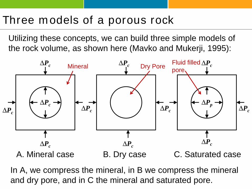
Three models of a porous rockUtilizing these concepts, we can build three simple models of the rock volume, as shown here (Mavko and Mukerji, 1995):
ΔPc ΔPc ΔPcMineral Dry Pore Fluid filled pore
ΔP ΔPΔP ΔPΔPc ΔPpΔPc ΔPcΔPc
ΔPc
ΔPcΔPcΔPc
A. Mineral case B. Dry case C. Saturated case
In A, we compress the mineral, in B we compress the mineral and dry pore, and in C the mineral and saturated pore.

Betti-Rayleigh Reciprocity
The Betti-Rayleigh reciprocity theorem states: “For an elastic body acted on by two different forces, the work y ydone by the first force acting on the displacements caused by the second force equals the work done by the second force acting on the displacements caused g pby the first force.”
Using the Betti-Rayleigh reciprocity theorem to compare cases A and B gives the following equation:compare cases A and B gives the following equation:
: where,11 += φKKK
modulus,bulk mineral modulus,bulk rock dry ==φ
KKKKK
mdry
mdry
porosity.andstiffness, space poredry == φφK
Pore space stiffness and compressibility
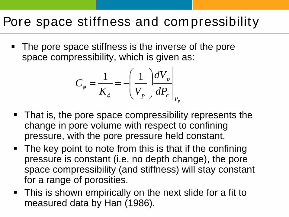
The pore space stiffness is the inverse of the pore space compressibility, which is given as:p p y g
p
dPdV
VKC
−== 11
φ
pPcp dPVK φ
That is, the pore space compressibility represents the change in pore volume with respect to confiningchange in pore volume with respect to confining pressure, with the pore pressure held constant.
The key point to note from this is that if the confining pressure is constant (i.e. no depth change), the pore space compressibility (and stiffness) will stay constant for a range of porosities.
This is shown empirically on the next slide for a fit to measured data by Han (1986).

Empirical fit to Han’s dataset
This figure (from Russell and SmithRussell and Smith, 2007) shows the fit of pore space stiffness to a set of measured values at constant confining
Kφ /Km = 0.162
RMSE 0 039g
pressure and differing porosity (Han 1986) where
RMSE = 0.039
(Han, 1986), where Kdry and Kφ have been normalized by di idi bdividing by Km.

Modeling Kdry versus porosity
To model Kdry at different porosities, the equation for the in-situ, or calibrated, Kdry can be re-arranged as follows: dry g
−=
mcaldrycal KKK1111
φφ mcaldrycal _φφ
The new value can be written: 1111
Th ti ll t li i t th
−=
mnewdrynew KKK1111
_φφ
These equations allows us to eliminate the pore space stiffness term and thus compute a new Kdry :
1111 φ
−+=
mcaldrycal
new
mnewdry KKKK1111
__ φφ

Modeling Kdry versus porosity
KmNote thatNote that Kφ reduces to Km at 0% porosity, as
Constant Kφ
curve
p y,it should.
Knew
φcalφnew
Kcal
Graphically, this shows that we can thus model Kdry at a new porosity φnew using a calibration porosity φcal.

Fluid pore space stiffness
Using the Rayleigh-Betti reciprocity theorem to compare the A (mineral) and C (fluid) cases shown earlier gives an equation involving Ksat, the saturated bulk modulus:
: where,~11 += φ
KKK
modulus,bulk mineral modulus,bulk rock dry ==φ
mdry
msat
KKKKKKK
stiffness, space pore fluid ~ =−
+= φφfm
fm
KKKK
KK
porosity.and modulus,bulk fluid == φfK
Note that this equation is identical in form to the dry pore tiff ti d f K 0 it d t th dspace stiffness equation, and for Kf = 0 it reduces to the dry
equation.

Deriving the Gassmann equation
We now have two relationships that relate the dry, saturated fluid and mineral bulk moduli to porosity andsaturated, fluid and mineral bulk moduli to porosity and pore space stiffness.
These can be re-arranged for Kφ as follows:
fmsatmdrym
KKKK
KKKKK
KKKK
K −
=
= φφ φφ :Sat.,:Dry
fmsatmdrym KKKKKK −
−
− φφ
Eliminating Kφ and dividing through by φ and Km gives us th f G (1951) tithe famous Gassmann (1951) equation:
fdrysat KKK +=)( fmdrymsatm KKKKKK −−− φ

The rock physics template (RPT)
Ødegaard and Avseth(2003) proposed a technique they called the rock physicsthe rock physics template (RPT), in which the fluid and mineralogical content ofmineralogical content of a reservoir could be estimated on a crossplot of Vp/Vs ratio against acoustic impedance, as shown here.
from Ødegaard and Avseth (2003)

The Ødegaard/Avseth RPT
Ødegaard and Avseth (2003) compute Kdry and μdry as a function of porosity φ using Hertz-Mindlin (HM) contact p y φ g ( )theory and the lower Hashin-Shtrikman bound:
4/1/1
−
−−=
−
HMcc
dK μφφφφ
,289
6 where,
34/1/
3)3/4()3/4(1
++=−
+
−−+
=
++
−
HMHMHMHM
ccdry
HMHMmHMHM
dry
KKz
KKK
μμμμ
μφφ
μφφμ
μμμ
,)1(2
)1(3)2(5
44 ,)1(18
)1(
263
31
22
22231
22
222
−−=
−=
+
++
mcmHM
mcHM
HMHMmHMy
PnPnK
Kzz
μφνμμφ
μμμ
member.-endporosity high andratio,sPoisson' mineral grain,per contacts ,modulusshear andbulk mineral ,,pressure confining
)1(2)2(5)1(18 2222
=====
−−
−
cm
mm
mmHM
mHM
nKPφν
μνπννπ
p yg,g ,p cm φ They then use standard Gassmann theory for the fluid
replacement process.

The Ødegaard/Avseth RPT
Here is the Ødegaard/Avseth RPT for a range of porosities and water saturations, in a clean sand case.

A pore space stiffness RPT
We propose a new approach to the rock physics template, in which we still use Gassmann for saturationtemplate, in which we still use Gassmann for saturation change but use pore space stiffness to compute the porosity change.Th l th thi d i th d f ti The only other thing we need is a method of computing shear modulus change.
Murphy et al. (1993) measured Kd and μ formeasured Kdry and μ for clean quartz sandstones, and found a constant of 0.9 for their ratio:their ratio:

Modeling μ versus porosity
As shown in the previous figure, the ratio of Kdry/μ is constant for varying porosity. Therefore, we could computeconstant for varying porosity. Therefore, we could compute the new value of μ using the equation:
K
situindry
newdrysituinnew K
K
−−=
_
_μμ
However, the formula above does not correctly predict the mineral value at 0% porosity. Our new approach is to use the same formulation as for the bulk modulus:
−+= newφ 1111
the same formulation as for the bulk modulus:
−+=mcaldrycalmnewdry μμφμμ __

The pore space stiffness RPT
Here is the pore space stiffness RPT for a range of porositiesHere is the pore space stiffness RPT for a range of porosities and water saturations, where we have calibrated the curves at 20% porosity.

A comparison of the two methods
Here is a comparison of the pore space stiffness method (red) p p p ( )and the Ødegaard and Avseth method (blue). At the calibration value for a porosity of 20% (black), the curves are identical.

Comparison of the methods for the modulus ratio A comparison between the two methods and the constant ratio empirical
result. The plot on the left shows the dry rock Κ/μ ratio as a function of it (0 t 40%) d th l t th i ht h th d hporosity (0 to 40%) and the plot on the right shows the dry shear
modulus as a function of porosity for only the first 10% of porosity:
The new approach is closer to the experimental results of Murphy et al., except near 0% porosity, where it correctly predicts the mineral value.

Vp/Vs vs P-impedance from logs
Now we will Shales
3.0
Now we will compare our templates to
l d t Thi atio
real data. This plot shows well log data from a V
p/V
s ra
Brine sands
Cemented sands
ggas sand in the Colony area of Alberta Gas sands5
The Vp and ρ logs were measured and Vs was computed using
Alberta.
P-impedance (m/s*g/cc)
Gas sands
4500 11000
1.5
The Vp and ρ logs were measured and Vs was computed using the mud-rock line in the shales and wet sands and the Gassmann equations in the gas sands.

Vp/Vs vs P-impedance from inversionThe results of a simultaneous Shales2.
9
pre-stack inversion from the same area.
Brine sandsCemented sands
atio
Note that the range of values is less extreme
Vp/
Vs
ra
is less extreme than on the log data due to the bandlimited nature of the seismic data.
Gas sands
P-impedance (m/s*g/cc)5200
1.8
6800P-impedance (m/s g/cc)
Next, we show the log and seismic data superimposed on the RPTs, where the log data has been integrated to time.

Avseth/Ødegaard Rock Physics Template
30% Porosity 20% Porosity Seismic (Vp/Vs shifted) Log data

New Rock Physics Template
30% Porosity 20% Porosity Seismic (Vp/Vs shifted) Log data

New Rock Physics Template
30% Porosity 20% Porosity Seismic (Vp/Vs shifted) Log data

Pressure changes
A plot of Kφ /Km vs log(press re) for thelog(pressure) for the Han dataset at different pressures, with the l t fitleast-squares fit:
)l (02700650 PK
+φ
F thi R ll d S ith (2007) d i l ti hi
)ln(027.0065.0 PKm
+=φ
From this, Russell and Smith (2007) derive a relationship between change in pore space stiffness and pressure, which can be used to alter pressure in the new template:
PPKK m /027.0 Δ=Δ φ

Conclusions In this talk, we proposed a new approach to the computation
of a rock physics template using pore space stiffness. We showed how pore space stiffness could be used to
estimate the dry rock bulk modulus as a function of porosity, used a similar equation for shear modulus and from thisused a similar equation for shear modulus, and from this developed the new template.
Comparing the new template to the Ødegaard and Avsethapproach using lab, measured log and seismic data: The template fits are both reasonable, and quite similar. The pore space stiffness method gives a better fit to the Murphy et al.The pore space stiffness method gives a better fit to the Murphy et al.
(1993) lab data. Pressure changes can be modeled empirically. The new method is based on the physics of the reservoir and passes The new method is based on the physics of the reservoir and passes
Occam’s razor: “All things being equal, simpler explanations are generally better than more complex ones”.

Acknowledgements
We wish to thank the CREWES sponsors and our colleagues at Hampson-Russell, CGGVeritas, and CREWESCREWES.
BR would like to especially thank Qing Li, who was the p y gone who said to me: “Why not use the same equation for changing shear modulus as you do for bulk modulus” which should have been obvious to me butmodulus , which should have been obvious to me, but wasn’t!

ReferencesGassmann, F., 1951, Uber die Elastizitat poroser Medien: Vierteljahrsschriftder Naturforschenden Gesellschaft in Zurich, 96, 1-23.
Han, D., 1986, Effects of porosity and clay content on acoustic properties of sandstones and unconsolidated sediments: Ph.D. dissertation, Stanford.
Mavko, G., and T. Mukerji, 1995, Seismic pore space compressibility and Gassmann's relation: Geophysics, 60, 1743-1749.
M h W R i h A d H K 1993 M d l D iti fMurphy, W., Reischer, A., and Hsu, K., 1993, Modulus Decomposition of Compressional and Shear Velocities in Sand Bodies: Geophysics, 58, 227-239.
Ødegaard, E. and Avseth, P., 2003, Interpretation of elastic inversion results using rock physics templates: EAGE, Expanded Abstracts.
Russell, B. H. and Smith, T., 2007, The relationship between dry rock bulk modulus and porosity – An empirical study: CREWES Report, Volume 19.


