Supplementary Materials for

“A Decomposition Method Based on a Model of Continuous Change”

by Shiro Horiuchi, John R. Wilmoth and Scott D. Pletcher

Demography Vol. 45, No. 4 (November 2008), pp. 785-801.

*

Table of Contents

Introduction 1

1 Example 3: Demographic transition in Sweden 2

2 Example 4: Sex difference in the longevity of bean beetles 5

3 Sensitivity analysis 8

4 Appendix A: Measuring discrepancies between two vectors 12

5 Appendix B: MATLAB program 13

References 14

Tables and Figures 16

Introduction

This manuscript comprises a few sections and appendices that were included in some early versions

but not in the final version of the article entitled “A Decomposition Method Based on a Model of

Continuous Change” by Shiro Horiuchi, John R. Wilmoth and Scott D. Pletcher. The article has been

published in Demography, Vol. 45, No. 4 (November 2008), pp. 785-801. Because the article is cited

for a number of times in this manuscript, we refer to it simply as HWP.

It is assumed that readers of this manuscript have already read HWP, which presents a new,

general method (the line integral method) of decomposition analysis. Two application examples of the

method (Example 1 and Example 3) are given in HWP. Additional two examples (Example 3 and

Example 4) are shown in Sections 1 and 2 of this manuscript. The four examples, together with the

previous studies using the method (Glei and Horiuchi 2007; Pletcher et al., 2000; Wilmoth and

Horiuchi 1999; Wilmoth et al., 2000), demonstrate the flexibility and wide applicability of the method.

Section 3 examines the sensitivity of the method with respect to departures from the assumption

of proportionality. Appendix A explains an indicator used in Section 3, which has been devised for

measuring discrepancies between two vectors, and Appendix B displays a MATLAB program for the

method.

1

1. Example 3: Demographic transition in Sweden

In economically developed countries, mortality and fertility changed markedly during the last two

centuries, thereby affecting the rate of population growth. However, levels of mortality and fertility by

age are not directly reflected in the observed rate of population growth, which is affected as well by the

age structure of the population and by migratory flows. The intrinsic rate of population growth, on the

other hand, is determined solely by current regimes of mortality and fertility, as expressed by Lotka’s

well-known equation:

, (1) 1)()(0

=∫∞ − dxxmxe rx l

where r is the intrinsic growth rate, is the proportion of survivors from birth to exact age x in the

current life table, and is the current birth rate at exact age x. Because we are interested in

assessing effects of the mortality function rather than those of the survivor function, the following

expression represents the decomposition problem more clearly:

)(xl

)(xm

, (2) 1)(0

)(0 =∫∞ ∫−− dxxmee

x dyyrx μ

where )(yμ is the force of mortality, or the instantaneous death rate, at exact age y.

In this example, we investigate the effects of changing mortality and fertility on trends in the

intrinsic growth rate for the female population of Sweden during 1778-2002 using data from a previous

study (Horiuchi 1995) supplemented with information on recent fertility (Statistics Sweden 2007) and

mortality (HMD 2007). Changes in the intrinsic growth rate were decomposed into effects of death

rates for ten 5-year age groups (0-4, 5-9, ..., 45-49) and birth rates for seven 5-year age groups (15-

19, ..., 45-49). Fertility outside this age range is negligible, and mortality at post-reproductive ages has

no effect on the intrinsic growth rate. Between two consecutive 5-year periods, all changes in age-

specific birth rates and logarithms of age-specific death rates were assumed proportional to each other.

2

Thus, the line integral method of decomposition analysis was applied to each of the 44 pairs of

successive 5-year time periods. The number of intervals, N, used for numerical integration was set at

four. Thus, the entire period was divided into 176 (4x44) intervals. In this analysis, N=4 turned out to

be large enough to produce sufficiently accurate results. The absolute proportional error (ε ) was less

than one percent except for seven of the 44 pairs (in all seven cases, the intrinsic growth rate remained

virtually unchanged between two successive periods, making the denominator of the fraction in Eq. (8)

of HWP almost zero).

Effects of the ten age-specific death rates and of the seven age-specific birth rates can be

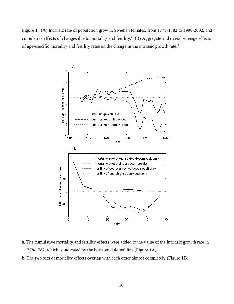
aggregated to obtain the total effects of mortality and fertility, respectively. Cumulative effects of

mortality and fertility changes since 1778-1782 are shown in Figure 1A. In each 5-year time period,

the sum of cumulative mortality (dash-dot line) and fertility (dashed line) effects equals the change in

the intrinsic growth rate between 1778-1782 and the period in question (i.e., the difference between the

solid curve and the horizontal dotted line). Overall, the intrinsic growth rate (per annum) decreased

from 0.59 percent in 1778-1782 to –0.96 percent in 1998-2002 because the negative effects of fertility

decline (-3.41) exceeded the positive effects of mortality reduction (1.86). Figure 1B displays the

effects of changing age-specific birth (dashed line) and death rates (solid line) on the overall change in

the intrinsic growth rate between 1778-1782 and 1998-2002. The greatest positive effect is found for

the death rate at ages 0-4, and pronounced negative effects are seen for birth rates in the 20’s and 30’s

of age.

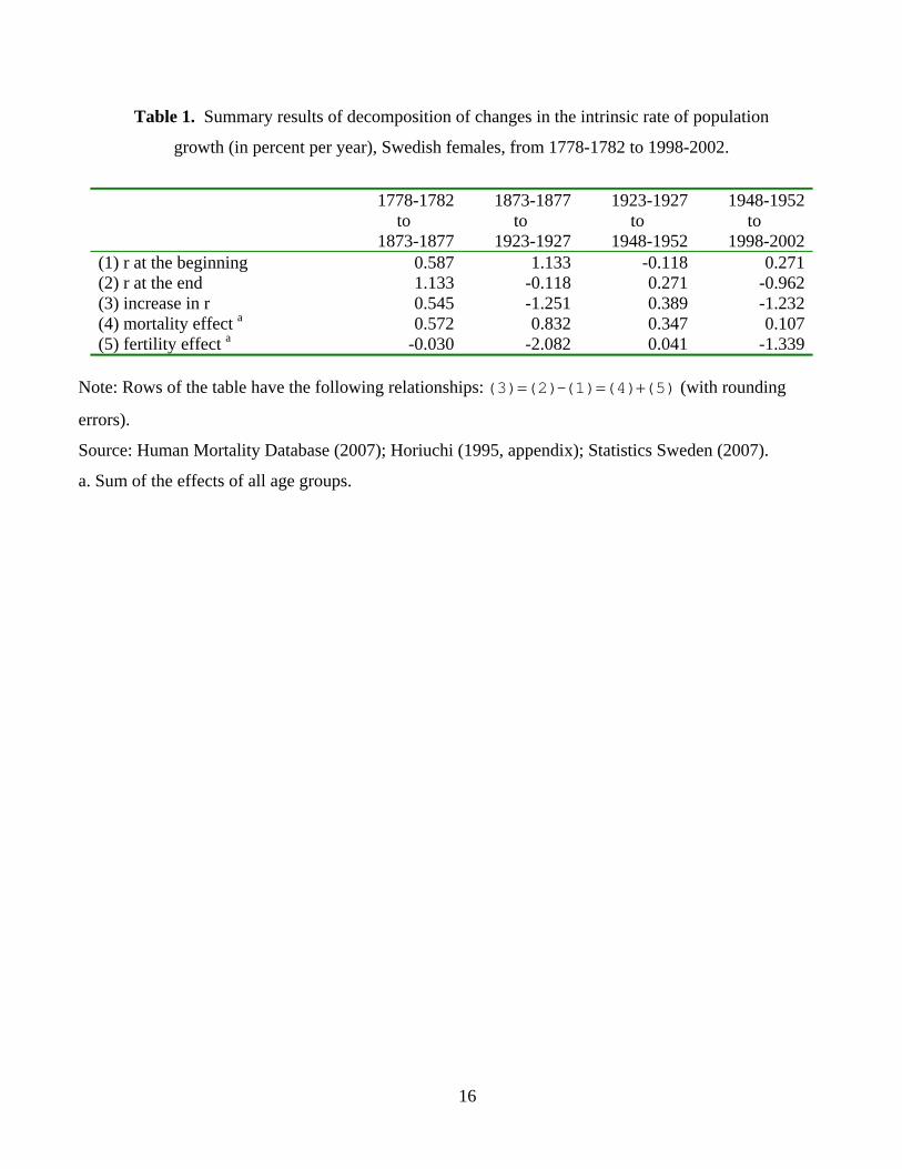
These decomposition results suggest that population dynamics of Sweden during this 225-year

time period can be divided into four distinct phases, as summarized in Table 1. In the first phase,

mortality reduction, especially at young ages, resulted in a substantial increase in the intrinsic rate of

population growth (per annum) from 0.59 percent in 1778-1782 to 1.13 percent in 1873-1877. In the

3

second phase, however, fertility decline led to an enormous reduction in the intrinsic growth rate,

which fell to –0.12 percent in 1923-1927.

The third phase, 1923-1927 to 1948-1952, is characterized by two idiosyncratic historical events,

the Great Depression and World War II. This special period witnessed a downturn and an upturn due

to strong temporary effects of these two events, rather than long-term trends. The economic crisis

brought even lower fertility, which reduced the intrinsic growth rate further to –1.00 percent in 1933-

1937, although the end of the war and the post-war Baby Boom raised fertility again, yielding positive

values for the intrinsic growth rate of 0.48 percent in 1943-1947 and 0.27 percent in 1948-1952.

The final phase is after World War II. The intrinsic growth rate, after being slightly positive

during most of the 1950s and 1960s, became negative again due to below-replacement fertility in the

following decades. To anyone familiar with the population history of Sweden or Western Europe in

general, these conclusions are hardly surprising, but they are now supported by simple quantitative

results linking changes in age-specific mortality and fertility rates to changes in the intrinsic rate of

population growth.1

.

1 Keyfitz (1968:189) partitioned the change in the intrinsic growth rate in Australia into three

components: fertility, mortality, and their interaction. For fertility and mortality, only total effects (not

age-specific effects) were computed, because interaction terms would be complicated if the procedure

had been used for deriving age-specific mortality and fertility effects. The present method, however,

makes it possible to derive age-specific effects without producing interaction terms.

4

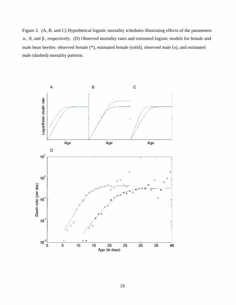
2. Example 4: Sex difference in the longevity of bean beetles

Females tend to live longer than males. This has been observed for many human populations as

well as a number of other species. Is this mainly because (a) males have consistently higher mortality

than females throughout most phases of the life, (b) males have higher mortality risks than females

particularly at old ages, or (c) mortality rates rise faster with age in males than in females? In this

discussion, we separate old ages from other ages because the age pattern of mortality in old ages

differs noticeably from the pattern at younger ages: the age-related mortality rise tends to level off at

old ages in virtually every species whose mortality patterns have been investigated with a large number

of old individuals (Vaupel et al. 1998).2

The data produced by Tatar and Carey (1994) provide an opportunity to investigate this question

for bean beetles. These authors recorded deaths in two generations of bean beetles raised under

controlled conditions. In both cohorts, females lived significantly longer, on average, than males. In

the older generation, for example, the average length of life was 24.1 days for females and 14.6 days

for males.

We investigated this sex differential using a logistic model of mortality. It has been shown that

logistic models fit mortality patterns of various species well, including humans at adult ages (Horiuchi

and Coale 1990; Thatcher, Kannisto and Vaupel 1998). In particular, a three-parameter version of the

logistic equation accurately represents age variations of mortality in two species of flies: the common

2 Although the distinction between childhood mortality and adult mortality is important for analyzing

sex differentials in the life expectancy of humans, it is not necessarily so for a number of other species.

For some egg-laying species, it is very difficult to distinguish defective eggs from deaths after hatching

out of eggs, and mortality on the first day is thus ignored. For some species that go through

metamorphosis, mortality immediately after eclosion from pupa is negligibly low in laboratory settings.

5

fruit fly, Drosophila melanogaster (Fukui et al. 1996; Pletcher et al. 2000; Promislow et al. 1996), and

Mediterranean fruit flies (Wilson 1994, using data from Carey et al. 1992). We adopted this model

because the age patterns of mortality (Figure 2D) in the bean beetle populations of Tatar and Carey,

and the trajectories of their life table aging rate3 (not shown here), appeared highly consistent with the

logistic equation.4

In the logistic model, the force of mortality, or instantaneous death rate, at exact age x is given by

)1(1

)(−+

= x

x

eex

θ

θ

αβαμ . (3)

The three parameters of the model can be interpreted as follows: α is the force of mortality at age

zero and represents the overall level of mortality throughout most of the life span (except for very old

ages); β/1 is the level of the mortality plateau at very old ages; and θ indicates the pace of

(exponential) mortality increase with age. Hypothetical mortality curves illustrating the effects of

these parameters are shown in Figures 2A, 2B and 2C. Thus, α , β , and θ correspond to the possible

3 The concept and characteristics of the life table aging rate are discussed by Horiuchi and Wilmoth

(1997) and its use for assessing mortality models has been demonstrated by Horiuchi and Coale (1990). 4 The fitness of the logistic model to these data can be compared with those of other models using the

likelihood ratio test (Pletcher 1999). The test was not conducted here because the two pieces of visual

evidence (i.e., age trajectories of logarithmic mortality and that of the life table aging rate) suggested

strongly that the logistic model should be more appropriate than some other widely used models such

as Gompertz and Makeham.

6

explanations for sex differentials in mortality that were mentioned earlier (i.e., (a), (b), and (c),

respectively).5

Maximum likelihood estimates of the three parameters were obtained for the female and male

cohorts of bean beetles by fitting the age distribution of deaths implied by the logistic model to the

observed age distribution. Often, mathematical models are fitted directly to age-specific death rates

using ordinary or weighted least squares. However, the maximum likelihood approach is more

appropriate than these conventional methods if the age distribution of deaths for the cohort is available

(Promislow et al. 1999; Pletcher 1999). Both the estimated logistic curves and the observed death rates

for females and males are shown in Figure 2D.

The sex difference in the life expectancy of bean beetles was decomposed into four elements,

consisting of the effects of differences in the three parameters and of disparities between observed life

expectancies and those implied by the fitted logistic models. For these calculations, the number of

intervals, N, was set at 100, and the proportional error of the decomposition, ε , was 0.0006 percent.

The results in Table 2 suggest that about 55 percent of the sex difference is due to θ (the pace of age-

related mortality increase), 40 percent is attributable to α (the overall mortality level), and only 5

percent results from β (the mortality plateau level). Thus, male bean beetles may senesce significantly

faster than females, and this sex difference in the rate of aging is the primary cause of the sex

difference in life expectancy. The decomposition method enables us to quantify and compare the

effects of different aspects of the mortality trajectory on the sex differential in life expectancy.

5 Several researchers have specified the three-parameter logistic model in different ways. Those

specifications are mathematically equivalent but the parameters are differently interpreted. Equation

(3) is a modified version of the formulation by Vaupel (1990).

7

3. Sensitivity Analysis

In principle, the line-integral method of decomposition analysis can be used in combination with

any assumption about relationships among changes of covariates. However, in practice, it is convenient

to adopt the assumption that changes in all covariates are in fixed proportions to one another

throughout the interval, which seems to be the simplest and most neutral assumption. Because the

method is based on the very general relation, ( ) ( ( ))y t f t= x , it is difficult to examine analytically the

sensitivity of decomposition results with respect to deviations from the proportionality assumption.

Therefore, in this section, we attempt to evaluate the sensitivity using Examples 1 and 3.6

Each example covers a number of consecutive periods (55 calendar years in Example 1, and 45

quinquennia in Example 3). In each case, it is possible to apply the decomposition method in two

distinct manners: either by examining changes between the first and last sets of observations only, or

by examining changes in each pair of successive 1- or 5-year periods and then aggregating effects

across the entire period. While an assumption of proportional change among all covariates seems

reasonably plausible over short time periods, the same assumption appears less well justified when

applied over a period of several decades or even centuries. Thus, by comparing these two means of

applying the decomposition technique, we can evaluate the sensitivity of the results to departures from

the assumption of proportional increments. Table 1 of HWP and table 1 of this manuscript showed the

second kind of results for Examples 1 and 3 (aggregated effects from multiple short-period

decompositions), which are now compared with the first kind (overall effects from a single long-period

decomposition).

6 Example 2 or 4 cannot be used for this purpose, because in those examples, t is a hypothetical

dimension of change between the two populations.

8

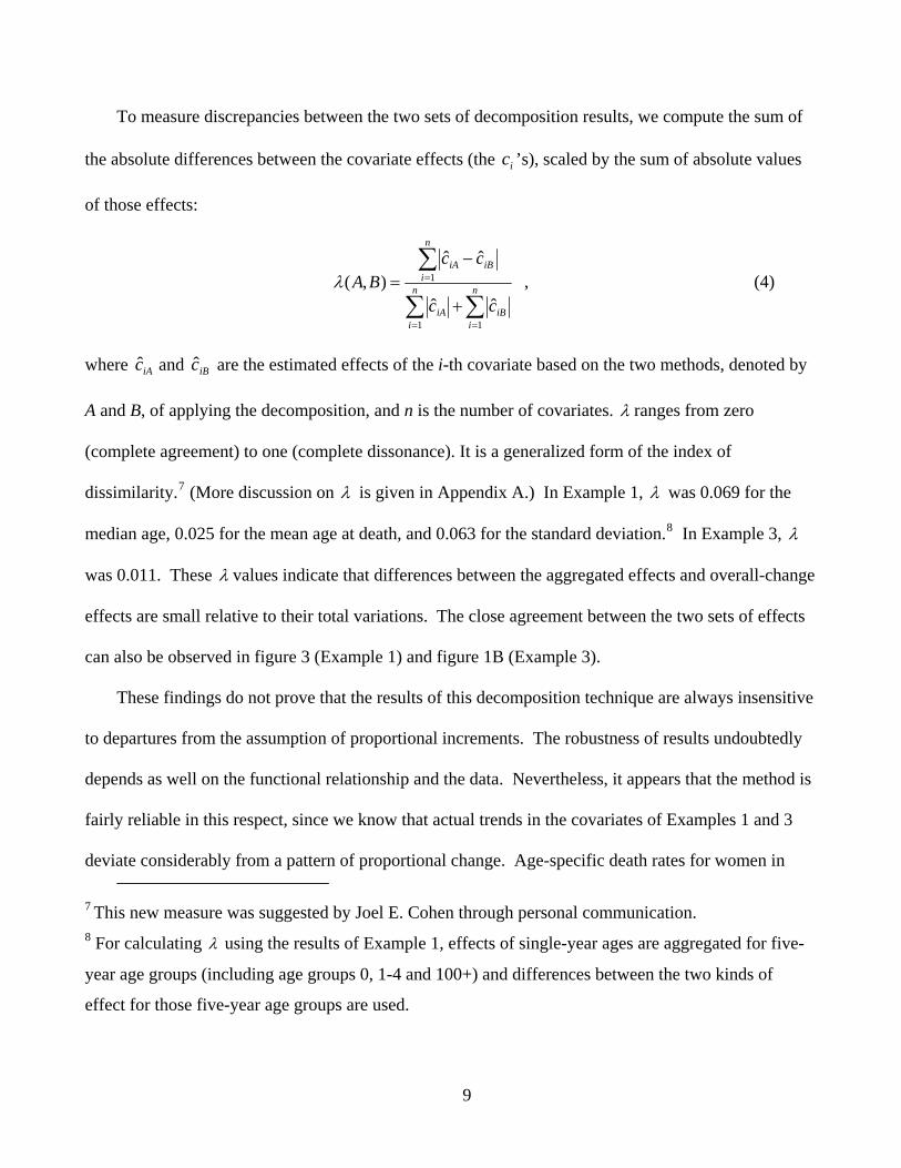
To measure discrepancies between the two sets of decomposition results, we compute the sum of

the absolute differences between the covariate effects (the ’s), scaled by the sum of absolute values

of those effects:

ic

∑∑

∑

==

=

+

−= n

iiB

n

iiA

n

iiBiA

cc

ccBA

11

1

ˆˆ

ˆˆ),(λ , (4)

where and are the estimated effects of the i-th covariate based on the two methods, denoted by

A and B, of applying the decomposition, and n is the number of covariates.

iAc iBc

λ ranges from zero

(complete agreement) to one (complete dissonance). It is a generalized form of the index of

dissimilarity.7 (More discussion on λ is given in Appendix A.) In Example 1, λ was 0.069 for the

median age, 0.025 for the mean age at death, and 0.063 for the standard deviation.8 In Example 3, λ

was 0.011. These λ values indicate that differences between the aggregated effects and overall-change

effects are small relative to their total variations. The close agreement between the two sets of effects

can also be observed in figure 3 (Example 1) and figure 1B (Example 3).

These findings do not prove that the results of this decomposition technique are always insensitive

to departures from the assumption of proportional increments. The robustness of results undoubtedly

depends as well on the functional relationship and the data. Nevertheless, it appears that the method is

fairly reliable in this respect, since we know that actual trends in the covariates of Examples 1 and 3

deviate considerably from a pattern of proportional change. Age-specific death rates for women in

7 This new measure was suggested by Joel E. Cohen through personal communication.

8 For calculating λ using the results of Example 1, effects of single-year ages are aggregated for five-

year age groups (including age groups 0, 1-4 and 100+) and differences between the two kinds of

effect for those five-year age groups are used.

9

Japan followed markedly different trajectories between 1950 and 2004: the decline of old-age

mortality accelerated, while the reduction of mortality at other ages slowed down. Likewise, mortality

and fertility in Sweden changed through entirely different paths between 1778-1782 and 1998-2002:

mortality declined through most of the periods, whereas fertility decreased, increased, or remained

nearly constant in different periods.

Another issue about the assumption of proportional increments is that some mathematical

transformations of the covariates ( ’s) may meet the condition better than the covariates in their

original scale ( ’s). For example, changes in the logarithm of age-specific death rates may be more

closely proportional to each other than changes in the original death rates. Thus, a more general form

of the assumption of proportional increments given in Eq. (7) of HWP is

)( ii xh

ix

)())(())(())(())((

12

1 tgtxhtxhtxhtxh

iiii

iiii =−− , for any i. (5)

Note that the function h has a subscript i because different transformations may be applied to each

covariate.

We arbitrarily selected five transformations – , , , , and x itself – and obtained

covariate effects for Examples 1 and 3. As described earlier, data for each of these examples comprise

observed values of the dependent variable and its covariates for a number of consecutive periods. In

this experimental calculation, however, only the first and last sets of observations were used as inputs

to the decomposition analysis. Then the long-term change in the dependent variable between the two

periods was decomposed assuming proportional changes in the selected functional form of the

covariates. The five sets of decomposition results ( ’s ) produce ten

)ln(x

ic

xe 3x 3/1 x

λ values, because ten different

combinations of two functions can be chosen from the five transformations.

10

The decomposition results did not differ in a substantial or meaningful way among these

transformations. In Example 1, λ was below 0.05 for 26 of the 30 pairs (10 pairs for each of median,

mean, and standard deviation), with a maximum of 0.066 for the median age at death. In Example 3,

λ was below 0.05 in all 10 cases. Thus, differences in decomposition results associated with

alternative transformations of the covariates do not appear to have practical significance, at least for

the data and functions considered here.

11

4. Appendix A: Measuring Discrepancies between Two Vectors

Discrepancies between two sets of decomposition results (two real-numbered vectors of the same size)

cannot be summarized by the correlation coefficient or the index of dissimilarity. The correlation

coefficient indicates the extent of linear relationship, but not the extent of exact agreement, between

two real-numbered vectors. The index of dissimilarity (Duncan and Duncan 1955) compares two

probability distributions but does not deal with vectors that have negative elements.

A more appropriate measure is given by:

∑∑

∑

==

=

+

−= n

iiB

n

iiA

n

iiBiA

cc

ccBA

11

1

ˆˆ

ˆˆ),(λ . (B1)

where ’s and ’s are elements of the two real-number vectors, A and B. iAc iBc ),( BAλ ranges from zero

to one. ), BA(λ is zero if the two vectors are identical. ),( BAλ is one if the two vectors are completely

dissonant in the sense that the sign (+, 0, -) of and the sign of are different for every i. iAc iBc

),( BAλ is a generalization of Dbrushin’s coefficient, which measures the maximum difference

among multiple probability distributions and is computed as ∑=

−n

iiBiABA

pp1,2

1 max , where for any

(i, A) and for any A (Cohen, Kemperman, and Zbaganu 1998). When only two distributions

are compared, Dbrushin’s coefficient becomes the index of dissimilarity.

0≥iAp

1=iAp1∑=

n

i

),( BAλ is an extension of

the index of dissimilarity from probability distributions to real-numbered vectors.

12

5. Appendix B: MATLAB program

A short program of this decomposition method, written in MATLAB 6.1, is attached below. The

algorithm is explained in the appendix of HWP. In writing this program, priority was given to clarity

and understandability, rather than computational efficiency. The user has to provide a function with the

dependent variable as its output and the covariates as its input. The name of the function is contained

in a string variable fun. Two column vectors, x1 and x2, contain the covariates for the two sets of

observations, and y1 and y2 are corresponding values of the dependent variable. Other variables in

the program are as follows: n is the number of covariates, N is the number of intervals for numerical

integration, w contains parameters that the function may need in addition to the covariates, and delta

is a column vector containing ’s. The estimated contributions of the covariates ( ’s) will be

returned as a row vector, called c.

ixΔ ic

function c=decom(fun,x1,x2,N,w) eval(['y2=',fun,'(x2,w);']) eval(['y1=',fun,'(x1,w);']) d=x2-x1;n=length(d);delta=d/N; x=x1*ones(1,N)+(d*ones(1,N).*(ones(n,1)*[0.5:N-0.5]/N)); cc=zeros(n,N); for j=1:N,for i=1:n z=zeros(n,1);z(i)=delta(i)/2; eval(['cc(i,j)=',fun,'(x(:,j)+z,w)-',fun,'(x(:,j)-z,w);']) end,end disp(‘Error of decomposition (in %) ’) e=100*(sum(sum(cc))/(y2-y1)-1) disp(‘Effects of covariates ’), c=sum(cc') return

13

References

Carey, J.R., P. Liedo, D. Orozco, and J.W. Vaupel. 1992. “Slowing of Mortality Rates at Older Ages in

Large Medfly Cohorts.” Science 258:458-61.

Cohen, J. E., J. H. B. Kemperman and G. Zbaganu. 1998. Comparisons of Stochastic Matrices, with

Applications in Information Theory, Statistics, Economics and Population Sciences. Boston, Basel

& Berlin: Birkhäuser.

Duncan, O.D., and B. Duncan. 1955. “A methodological analysis of segregation indexes.” American

Sociological Review 20: 210-217.

Fukui, H. H., L. Ackert, and J. W. Curtsinger. 1996. “Deceleration of age-specific mortality rates in

chromosomal homozygotes and heterozygotes of Drosophila melanogaster.” Experimental

Gerontology 31(4):517-531.

Glei, D. and S. Horiuchi. 2007. “The narrowing sex gap in life expectancy: Effects of sex differences

in the age pattern of mortality.” Population Studies, 61:141-159.

Horiuchi, S. 1995. “The cohort approach to population growth: a retrospective decomposition of

growth rates for Sweden.” Population Studies 49:147-163.

Horiuchi, S. and A.J. Coale. 1990. “Age Patterns of Mortality for Older Women: an Analysis Using the

Age-specific Rate of Mortality Change with Age.” Mathematical Population Studies 2:245-267.

Horiuchi, S. and J.R. Wilmoth. 1997. “Age Patterns of the Life-Table Aging Rate for Major Causes of

Death in Japan, 1951-1990.” Journal of Gerontology: Biological Sciences 52A:B67-B77.

Human Mortality Database (HMD). 2007. University of California, Berkeley (USA), and Max Planck

Institute for Demographic Research (Germany), Available at www.mortality.org. (Data were

downloaded on February 6, 2007).

Keyfitz, N. 1968. Introduction to the Mathematics of Population. Reading, MA: Addision-Wesley.

Pletcher, S. D. 1999. “Model fitting and hypothesis testing for age-specific mortality data.” Journal

of Evolutionary Biology 12(3):430-439.

Pletcher, S. D., A. A. Khazaeli, and J. W. Curtsinger. 2000. “Why do lifespans differ? Partitioning

mean longevity differences in terms of age-specific mortality parameters.” Journal of

Gerontology: Biological Sciences 55: B381-B389.

Promislow, D. E. L., M. Tatar, A. A. Khazaeli, and J. W. Curtsinger. 1996. “Age-specific patterns of

genetic variation in Drosophila melanogaster. I. Mortality.” Genetics 143:839-848.

14

Promislow, D. E. L., M. Tatar, S. D. Pletcher, and J. Carey. 1999. “Below threshold mortality:

implications for studies in evolution, ecology and demography.” Journal of Evolutionary Biology.

12(2):314-328.

Searle, S. R., G. Casella, and C. E. McCulloch. 1992. Variance Components. New York: Wiley and

Sons.

Statistics Sweden. 2007. Statistical Database. Available at http://www.scb.se/ . (The data were

downloaded on February 7, 2007.)

Tatar, M. and J. R. Carey. 1994. “Sex mortality differentials in the bean beetle: reframing the

questions” American Naturalist 144:165-175.

Thatcher, A. R., V. Kannisto, and J. W. Vaupel. 1998. The Force of Mortality at Ages 80 to 120.

Odense: Odense University Press.

Wilmoth, J. R. and S. Horiuchi. 1999. “Rectangularization revisited: Variability of age at death

within human populations.” Demography 36:475-495.

Wilmoth, J. R., L. J. Deegan, H. Lundström, and S. Horiuchi. 2000. “Increase in maximum life span

in Sweden, 1861-1999.” Science 289:2366-2368.

Wilson, D. L. 1994. “The analysis of survival (mortality) data: Fitting Gompertz, Weibull, and

logistic functions.” Mechanisms of Ageing and Development 74:15-33.

Vaupel, J. W. 1990. “Relative risks: Frailty models of life history data.” Theoretical Population.

Biology 37:220-234.

Vaupel, J. W., J. R. Carey, K. Christensen, T. E. Johnson, A. I. Yashin, N. V. Holm, I. A. Iachine, V.

Kannisto, A. A. Khazaeli, P. Liedo, V. D. Longo, Y. Zeng, K. G. Manton, and J. W. Curtsinger.

1998. “Biodemographic trajectories of longevity.” Science 280:855-60.

15

Table 1. Summary results of decomposition of changes in the intrinsic rate of population

growth (in percent per year), Swedish females, from 1778-1782 to 1998-2002.

1778-1782

to 1873-1877

1873-1877to

1923-1927

1923-1927 to

1948-1952

1948-1952to

1998-2002(1) r at the beginning 0.587 1.133 -0.118 0.271(2) r at the end 1.133 -0.118 0.271 -0.962(3) increase in r 0.545 -1.251 0.389 -1.232(4) mortality effect a 0.572 0.832 0.347 0.107(5) fertility effect a -0.030 -2.082 0.041 -1.339

Note: Rows of the table have the following relationships: = = +(3) (2)-(1) (4) (5) (with rounding

errors).

Source: Human Mortality Database (2007); Horiuchi (1995, appendix); Statistics Sweden (2007).

a. Sum of the effects of all age groups.

16

Table 2. Decomposition analysis of sex differentials in the life expectancy of bean beetles.

Females Males Effecta (in %) Expectation of life at eclosion (in days)

Observed 24.12 14.63 9.49 (100.0) Estimated b 24.11 14.64 9.48 ( 99.9) Error 0.01 -0.01 0.01 ( 0.1) Estimated values of the logistic parameters c α (x10,000) 0.2649 1.5315 3.80 ( 40.0) (0.1398) (0.9742) β 2.9397 2.2252 0.48 ( 5.1) (0.2118) (0.0474) θ 0.4047 0.5751 5.20 ( 54.8) (0.0271) (0.0488) Number of cases 843 829

Source: Tatar and Carey 1994, table 1.

a. Contribution to the observed sex difference in the expectation of life at eclosion.

b. The expectation of life was estimated using the logistic model.

c. Figures in parentheses under the estimated parameter values are their standard errors, computed by asymptotic approximation (Searle et al., 1992).

17

Figure 1. (A) Intrinsic rate of population growth, Swedish females, from 1778-1782 to 1998-2002, and

cumulative effects of changes due to mortality and fertility.a (B) Aggregate and overall-change effects

of age-specific mortality and fertility rates on the change in the intrinsic growth rate.b

a. The cumulative mortality and fertility effects were added to the value of the intrinsic growth rate in

1778-1782, which is indicated by the horizontal dotted line (Figure 1A).

b. The two sets of mortality effects overlap with each other almost completely (Figure 1B).

18

Figure 2. (A, B, and C) Hypothetical logistic mortality schedules illustrating effects of the parameters

, θ, and β , respectively. (D) Observed mortality rates and estimated logistic models for female and

male bean beetles: observed female (*), estimated female (solid), observed male (o), and estimated

male (dashed) mortality patterns.

α

19

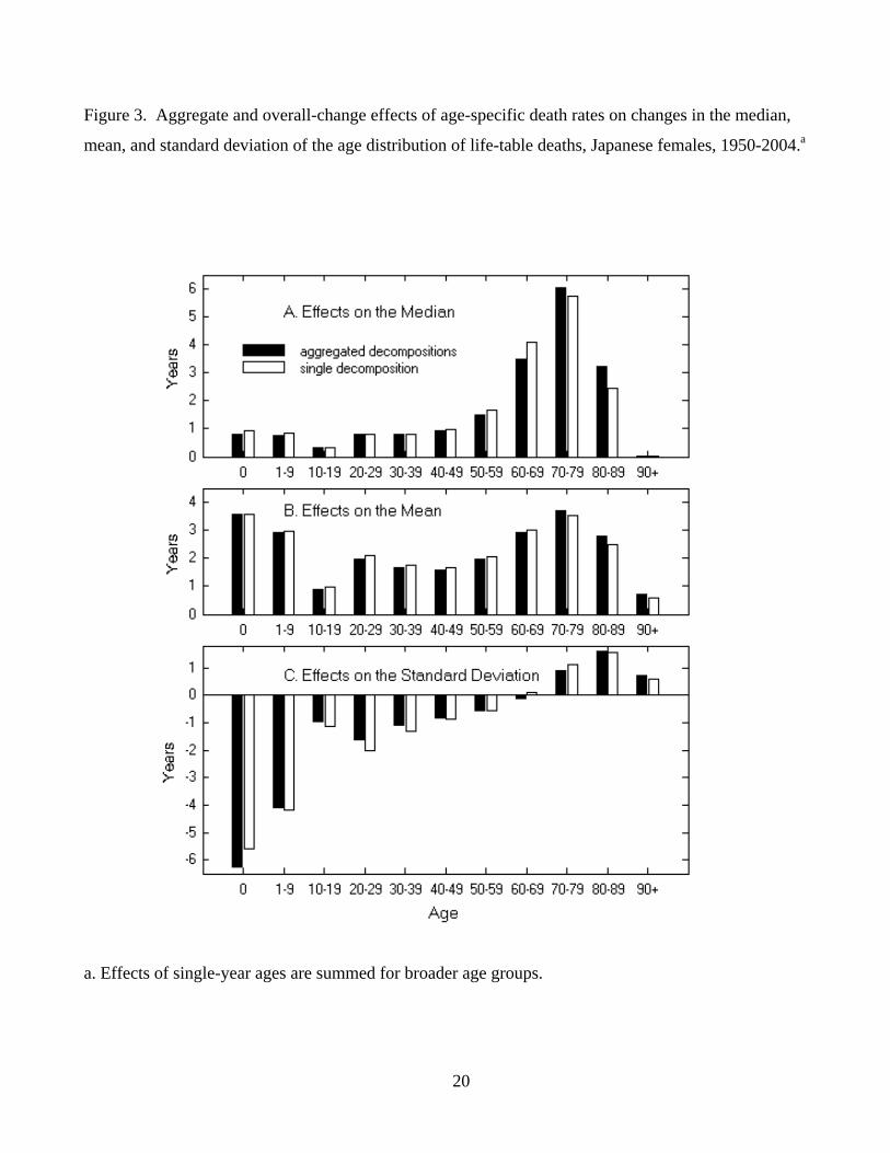
Figure 3. Aggregate and overall-change effects of age-specific death rates on changes in the median,

mean, and standard deviation of the age distribution of life-table deaths, Japanese females, 1950-2004.a

a. Effects of single-year ages are summed for broader age groups.

20