A generalized model of nonlinear viscoelasticity: applicationto the simulation of the brain shift.

Maya de Buhan1,2∗

Pascal Frey1,2

2 UPMC Univ Paris 06, UMR 7598, Laboratoire J.L. Lions, F-75005 Paris, France.1 Universidad de Chile, UMI 2807, Centro de Modelamiento Matemático, Santiago, Chile.

2010

Abstract

In this paper, we focus on the problem of modeling the deformation of cerebral structures,which are considered here to have a nonlinear viscoelastic behavior under external loads. Inthis context, we propose a generalized model of nonlinear viscoelasticity and present the nu-merical techniques used to solve it in three dimensions. Numerical results are then comparedwith experimental data, to show that our model is able to reproduce a behavior described inthe literature and to retrieve significant biophysical coefficients. Finally, we perform numeri-cal simulations on a complex brain domain, defined from imaging data and discretized usingtriangulations specifically adapted to its geometric properties (curvature).

1 IntroductionOver the last decades, the study of the mechanical properties of human tissues has been an activearea of research, especially focusing on the functional behavior of the skin, the lungs or the heart.However, the properties of biological soft tissues like the brain, the liver or the kidney have beenless investigated, maybe at the noticeable exception of ligaments and tendons, see Pena et al. [24],Provenzano et al. [25] and Jamison et al. [9]. Here we are mainly interested in modeling the brainstructure and we have rapidly noticed that there is no unique commonly acknowledged model.From our point of view, two communities have emerged from these investigations. On the onehand, authors advocate the use of a linear elastic model, sufficiently easy to solve efficiently toenvisage or to comply with real-time simulations, Bucki et al. [2], Wittek et al. [28], Ueno et al.[27]. On the other hand, nonlinear viscoelastic models are employed every time the requirementof an accurate simulation of the realistic behavior is preeminent over the computational expense,see Miller et al. [18, 19, 20], Wittek et al. [30], Darvish et Crandall [3] and the references therein.Additional models have also been proposed for specific purposes (poroelasticity Miga et al. [17]or plasticity) and nonetheless the limit between these types of models appears somehow artificial.Hence, we refer the reader to the quite complete literature review given by Libertiaux [14] andHrapko et al. [8]. Our approach is clearly inscribed in the second category of nonlinear models.

Indeed, in our previous work [4], we developed a nonlinear viscoelastic model (in large strains)obtained as the generalization of the model initially presented by Simo [26] and Lubliner [15] andmathematically analyzed in Le Tallec et al. [13, 12]. The model relies on the theory of standardmaterials which introduces internal state variables. We presented successively the discretization

∗e-mail: debuhan@ann.jussieu.fr

1

stages as well as the implementation of this model in three dimensions, with the aim of obtainingthe most accurate possible numerical results. The space discretization involves P0/P2 Lagrangefinite elements and the time discretization is based on an implicit Euler scheme. The linearizedversion of the resulting system derives naturally from a Newton method and is solved using anAugmented Lagrangian technique. To assess the numerical method, we evaluated the discrepancybetween a pseudo analytical solution and the solution computed on a simple domain.

In this article, we propose to use our model to simulate the deformations of brain structures.In a clinical context, such deformations may occur consecutively to a change of position of thepatient or during a neurosurgical procedure. Health care expectations are related to the ability ofthe model to predict the centimeter-scale motion or shift, Miga et al. [17], that occurs in surgeryand thus to participate actively to the treatment planning of surgical operations. In this context,the use of a quasi-static model seems to be adequate. Dynamical brain models are generally usedfor impact simulations, Brands et al. [1]. See Wittek, Joldes and Miller [29] [29, 11, 10] for efficientnumerical methods to solve dynamical models in real time.

This paper is divided in three parts. The first part presents the mechanical model and brieflydescribes the discretization stage and the numerical resolution. In the second part, numerical resultsare assessed through experimental results on swine brains in order to show that our model is ableto reproduce a complex behavior described in the literature and to retrieve relevant biophysicalconstitutive law. In the last part, we explain how we build triangulations especially adapted to thegeometric shape complexity of the computational domains at hand, defined from discrete imagingdata. Finally, we provide a three-dimensional example of numerical simulation of the brain shift.

2 The mechanical model and its numerical approximationAt first, we present the viscoelastic model in large strains that we used in numerical simulationsand we explain how our version differs and generalizes the classical model of [13].

2.1 The generalized modelLet Ω be a connected and bounded open set of R3 corresponding to the reference configuration. Wesuppose that the boundary Γ of Ω is Lipschitz-continuous. We assume also that the boundary canbe decomposed as Γ = Γ0 ∪ Γ1 with Γ0 ∩ Γ1 = ∅. The model problem we consider is the following:

Find the displacement vector u solving:−div T = f, in Ω,

u = u0, on Γ0,

T · n = g, on Γ1.

Here, f (resp. g) represents the body (resp. surface) forces, expressed in the reference configuration.The constitutive law is then given by the following relation, that relate the first Piola-Kirchhoffstress tensor T to the gradient of deformation F = Id+∇u:

T =dW

dF− pF−t. (2.1)

In the viscoelastic model we consider here, the internal energy W of the system can be written asfollows:

W (C,G1, ..., Gm) = W0(C) +

m∑i=1

Wi(C : Gi), m ∈ N∗, (2.2)

2

where the Cauchy-Green tensor C is defined as:

C = F tF = Id+∇u+∇ut +∇u · ∇ut,

and where the tensors Gi, for i ∈ J1,mK, are a finite number of internal variables used to measurethe deformation of dashpots embedded in the material. The evolution of these internal variables isdescribed by the set of following equations: νiG

−1i =

∂W

∂Gi+ qiG

−1i , in Ω,

Gi(0) = Id, in Ω,

∀i ∈ J1,mK, (2.3)

with νi, for i ∈ J1,mK, the viscosity coefficients. The pressures p and qi, for i ∈ J1,mK, occur-ing in equations (2.1) and (2.3) are the Lagrange multipliers associated to the incompressibilityconstraints:

det(F ) = det(Gi) = 1, ∀i ∈ J1,mK.

At this point, we observe that this model is slightly different from the model described in [13],in the sense that it contains supplementary internal variables, hereby justifying its denominationof generalized model. In other words, if the model of [13] is a nonlinear version of the Maxwellmodel, by analogy our model can be seen as a nonlinear version of the multi-mode Maxwell model.Its main strength relies on its versatility for handling complex behaviors (e.g. to account forvarious dissipation time) that could not be captured with the classical models. This rather complexformulation is indeed required by the application we have in mind, as will be emphasized in Section3. If we are well aware that such model is also more greedy in terms of computational cost, we arestill willing to use it for solving our complex problem.

For the sake of clarity, we remind the main stages of the discretization of our model and theresolution techniques that have been effectively implemented. We refer the reader to [4] for all thedetails. Let us point out that the authors have implemented all data structures, finite elementslibraries and nonlinear system resolution techniques using C language (about 10, 000 lines). Thesource code is available on demand to the corresponding author.

2.2 Space discretizationIn view of its numerical resolution using the finite element method, a weak formulation of the modelproblem shall be first written, which leads now to solve:

Find u− u0 ∈ V, p ∈ P, Gi ∈ H and qi ∈ Q, for ∀i ∈ J1,mK, such that:

∫Ω

(2F

∂W

∂C(C,G1, · · · , Gm)− pF−t

): ∇v dx

=

∫Ω

f · v dx+

∫Γ1

g · v dγ, ∀v ∈ V,∫Ω

p (det(F )− 1) dx = 0, ∀p ∈ P,∫Ω

(−∂Wi

∂y(C : Gi)C + νiG

−1i − qiG

−1i

): H dx = 0, ∀H ∈ H,∫

Ω

q (det(Gi)− 1) dx = 0, ∀i ∈ J1,mK, ∀q ∈ Q.

(2.4)

The functional spaces V,P,H and Q are chosen accordingly, i.e. such that all integrals are welldefined, y = C : Gi denotes here the argument of the function Wi and : denotes the double con-traction of tensors. Thus, the problem associates a nonlinear PDE endowed with incompressibilityconditions and m ODEs describing the time evolution of the internal variables.

3

Hereafter, we consider a conforming triangulation Th of the computational domain Ω where hrepresents the characteristic mesh size. The variational approximation of the initial problem (2.4)is classically obtained by replacing the functional spaces V, P, H and Q by finite dimensionalsubspaces Vh, Ph, Hh and Qh, respectively. We are well aware that the choice of these spaces is ofimportance to ensure the stability of the resolution. An analysis stage must confirm the validity ofthis choice, although it is out of the scope of this paper. Namely, we have retained the followingfinite elements spaces:

Vh =vh : Ω −→ R3, ∀K ∈ Th, vh|K ∈ P3

2, vh = 0 on Γ0

,

Ph = Qh =ph : Ω −→ R, ∀K ∈ Th, ph|K ∈ P0

,

Hh =Hh : Ω −→ U , ∀K ∈ Th, Hh|K ∈ P5

0

.

where U = H ∈ (M3)sym,det(H) = 1.

2.3 Time discretizationWe focus now on the time discretization of the problem using an implicit Euler scheme, whichis unconditionally stable. This is an essential requisite for dealing with the various time scalesoccurring in viscoelastic phenomena. Let ∆t be the time discretization step. The numerical schemewe considered leads to solve the following sequence of problems:

For n ∈ N, find un+1h − u0h ∈ Vh, pn+1

h ∈ Ph, Gn+1ih ∈ Hh and qn+1

ih ∈ Qh, for i ∈ J1,mK,solving:

∫Ω

(2Fn+1

h

∂W

∂C(Cn+1

h , Gn+11h , · · · , Gn+1

mh )− pn+1h (Fn+1

h )−t)

: ∇vh dx

=

∫Ω

f · vh dx+

∫Γ1

g · vh dγ, ∀vh ∈ Vh,∫Ω

ph(det(Fn+1h )− 1) dx = 0, ∀ph ∈ Ph,

νi(Gn+1

ih )−1 − (Gnih)−1

∆t− ∂Wi

∂y(Cn+1

h : Gn+1ih )Cn+1

h − qn+1ih (Gn+1

ih )−1 = 0,

det(Gn+1ih ) = 1, ∀i ∈ J1,mK, in each K ∈ Th,

endowed with the initial condition G0ih = Id, for i ∈ J1,mK.

The numerical resolution of this tedious problem is carried out in two steps. At first, we solvethe evolution equations of the internal variables and express the latter in terms of the unknownCn+1

h . As the resulting problem depends only on Cn+1h , it can then be solved as a classical nonlinear

elastic problem.

2.4 Calculation of the viscoelastic variablesAt each time step, we can compute each one of the m viscoelastic variables Gn+1

ih , for i ∈ J1,mK,independently, all contributing to the physical dissipation phenomenon. This can be achievedsolving the evolution equations in each element K in Th. To this end, we observe that the problemcan be rewritten, for each time step n ∈ N, as the following minimization problem:

Gn+1ih = arg min

H∈U

(Wi(C

n+1h : H) +

νi∆t

(Gnih)−1 : H

), ∀i ∈ J1,mK,

that can be computed, after some judicious transformations, using a classical Newton method.

4

2.5 Resolution of the elastic problemAccording to the relation Gn+1

ih = Gi(Cn+1h ), for i ∈ J1,mK, we can replace the viscoelastic variables

in the original problem (2.4). Let (φj)j=1..N be a basis of Vh and (ψj)j=1..M be a basis of Ph,respectively. If we consider the vector Un+1

h (resp. Pn+1h ) of the components of un+1

h − u0h (resp.pn+1h ) in the basis (φj)j=1..N (resp. (ψj)j=1..M ), our finite element problem takes, at each time stepn, the form of an algebraic system of N +M nonlinear equations with N +M unknowns:

Find (Un+1h , Pn+1

h ) ∈ RN × RM such that:

L(Un+1h , Pn+1

h ) = 0, in RN × RM ,

with the notations, for all (U,P ) ∈ RN × RM :

Lj(U,P ) =

∫Ω

2F∂W

∂C(C,G1(C), · · · ,Gm(C)) : ∇φj dx−

∫Ω

pF−t : ∇φj dx

−∫

Ω

f · φj dx−∫

Γ1

g · φj dγ, ∀j ∈ J1, NK,

Lj+N (U,P ) =−∫

Ω

ψj(det(F )− 1)dx, ∀j ∈ J1,MK.

This system can be very large but sparse. It can be linearized by a Newton algorithm. It iswell known that the Newton method is very sensitive to its initialization and may not converge insome cases, i.e. if the initial data differs largely from the solution. To overcome this drawback,the classical initialization strategy consists in using an incremental loading, Oden [23]. In thistechnique, the load acting on the body is applied as small increments. The equilibrium position isthen computed at the end of each load increment using as initial guess the position obtained at theprevious increment. At each iteration of the Newton method, the linear system can be solved byan augmented Lagrangian technique, Nocedal and Wright [22]. This iterative procedure consists inreplacing at each iteration step the initial linear system by a simplest system that can be solvedusing a preconditioned conjugate gradient.

2.6 ValidationThe aim of this section is to assess the numerical method by evaluating the discrepancy betweenthe approximate solution and a pseudo analytical solution computed in [4], in the case of thecompression of a cube fixed on one of its side (with slip conditions). Figures 1 illustrate the timeevolution of the pressure, the vertical constraint and one internal variable corresponding to thenumerical and the pseudo analytical solutions.

3 Efficiency of the generalized formulationOur objective is here to justify the choice of our mechanical model and to show its versatility inrecovering the relevant biophysical parameters. To this end, we compare the numerical results withthree experimental tests on swine brain tissues, published in three papers : Miller [18], Libertiaux[14] and Ning et al. [21]. In these tests, the geometry of the domain is non relevant as the biophysicalsamples correspond to simple shapes with axisymmetric property.

Let us point out that we extend the energy functional introduced in (2.2) as follows:

W0(C) = C01(I1(C)− 3) + C02(I2(C)− 3),

Wi(y) = Ci1(y − 3) + Ci2(y − 3)2, ∀i ∈ J1, 2K

5

0.0 0.5 1.0 1.5 2.0 2.5 3.0 3.5 4.01160

1180

1200

1220

1240

1260

1280

1300

Time (s)

Pres

sure

(N)

Analytical solutionNumerical solution

0.0 0.5 1.0 1.5 2.0 2.5 3.0 3.5 4.0!1100

!1050

!1000

!950

!900

!850

!800

!750

!700

!650

Time (s)

Lagr

ange

stre

ss (P

a)

Analytical solutionNumerical solution

(a) (b)

0.0 0.5 1.0 1.5 2.0 2.5 3.0 3.5 4.01.00

1.05

1.10

1.15

1.20

1.25

1.30

1.35

1.40

1.45

Time (s)

Inte

rnal

var

iabl

e

Analytical solutionNumerical solution

(c)

Figure 1: Evolution of (a) the pressure, (b) the vertical stress and (c) the vertical component ofthe second internal variable with respect to time during a compression test of 30%. Comparisonbetween the pseudo analytical solution (continuous line) and the numerical solution (crosses).

where the coefficients C are determined using a (least-square) curve fitting algorithm on experimen-tal data. This rather complex constitutive law is needed to be able to reproduce the biophysicalexperiments

The first experiment is directly inspired by the paper [18]. It corresponds to unconfined com-pressive tests on cylindrical samples (see Figure 2) at different strain rates. Figure 3 shows thecomparison between the experimental and the numerical solutions. Table 1 reports the coefficientsused to carry out these tests. We observe that both curves are well in accordance with each other.Notice that the stress-strain relation is nonlinear and depends on the strain rate. This is a clearindication of the nonlinear viscoelastic character of the brain tissues.

m C01 C10 C11 C12 ν1 C21 C22 ν2

2 0 145 0 1300 35000 150 2000 200

Table 1: Mechanical properties used for the first test case.

The second experiment has been performed on cylindrical samples (height 10 mm and diameter20 mm) and is reported in [14] . It consists in different tests in compression at different strain ratesand in relaxation. During the relaxation experiment, a compression stage at a rate of 0.1 s−1 is firstperformed, until a force of 0.5 N is achieved, then the relaxation constraint is measured while thecompression is held. Figure 4 shows the comparison between the experimental and the numerical

6

Figure 2: Configuration at rest (left). Deformed configuration with slip conditions (right).

!0.30 !0.25 !0.20 !0.15 !0.10 !0.05 !0.00!450

!400

!350

!300

!250

!200

!150

!100

!50

!0

True strain

Lagr

ange

stre

ss (P

a)

789eri:enta; s<;uti<n=u:eri>a; s<;uti<n

!0.30 !0.25 !0.20 !0.15 !0.10 !0.05 !0.00!1400

!1200

!1000

!800

!600

!400

!200

!0

True strain

Lagr

ange

stre

ss (P

a)9:;eri<enta= s>=uti>n?u<eri@a= s>=uti>n

(a) (b)

!0.30 !0.25 !0.20 !0.15 !0.10 !0.05 !0.00!3000

!2500

!2000

!1500

!1000

!500

!0

True strain

Lagr

ange

stre

ss (P

a)

678eri9enta: s;:uti;n<u9eri=a: s;:uti;n

(c)

Figure 3: Relation between the Lagrange stress and the true strain for three compression rates: (a)6.4 · 10−6 s−1, (b) 6.4 · 10−3 s−1, (c) 6.4 · 10−1 s−1. Comparison between the experimental solutionsreported by [18] (lines) and the numerical solutions (crosses).

solutions. Table 2 reports the coefficients used to carry out these tests. Here again, we observe thatboth curves are well in accordance with each other.

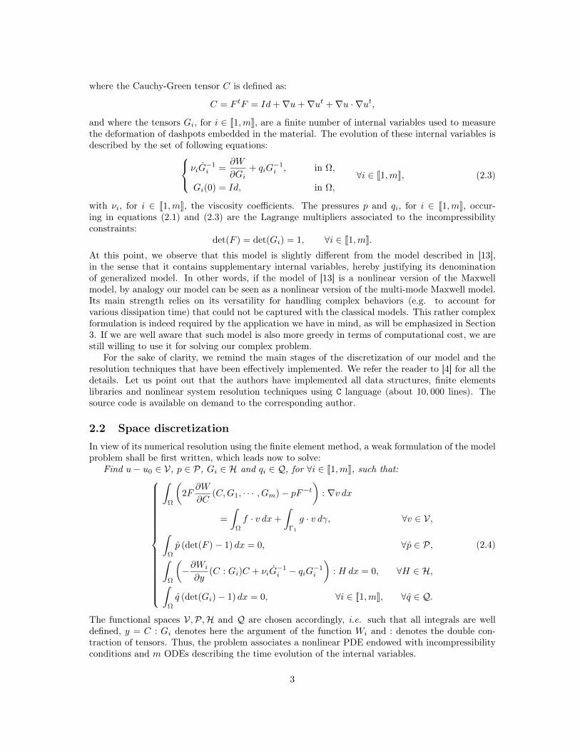
The third experiment is proposed in [21]. Shear stress tests at a 50% strain level have beencarried out on a porcine brainstem sample (13.41 × 6.49 × 1.05mm) to characterize its properties(see Figure 5). Table 3 reports the coefficients used for these tests. Figure 6 shows the comparisonbetween the experimental and the numerical solutions.

Once again, we observe that both curves are well in accordance with each other. These resultsclearly prove that our generalized model represents quite satisfactorily the biomechanical behaviorof the brain structures under a compressive load, for the relaxation test and under a shear load. Foreach experiment, we were able to find a suitable set of parameters to fit and validate the experimental

7

m C01 C10 C11 C12 ν1 C21 C22 ν2

2 0 150 0 200 5000 450 400 1500

Table 2: Mechanical properties used for the second test case.

!0.12 !0.10 !0.08 !0.06 !0.04 !0.02 !0.00!450

!400

!350

!300

!250

!200

!150

!100

!50

!0

True strain

True

stre

ss (P

a)

1.2 mm/min12 mm/min120 mm/min

1.2 mm/min12 mm/min120 mm/min

1.2 mm/min12 mm/min120 mm/min

(a)

0 10 20 30 40 50 600.0

0.1

0.2

0.3

0.4

0.5

0.6

Time (s)

Forc

e (N

)

Experimental solutionNumerical solution

0 50 100 150 200 250 300 350 400 450 5000.0

0.1

0.2

0.3

0.4

0.5

0.6

Time (s)

Forc

e (N

)Experimental solutionNumerical solution

(b) (c)

Figure 4: (a) Relation between the true stress and the true strain for three compression velocities.(b)(c) Evolution of the force with respect to time during the relaxation. Comparison between theexperimental solutions reported by [14] (lines) and the numerical solutions (crosses).

m C01 C10 C11 C12 ν1 C21 C22 ν2

2 0 6 30 0 100 200 0 1

Table 3: Mechanical properties used for the third test case.

data at best. We are well aware however that the experimental conditions, undoubtedly differentfrom one author to another, impact largely the biophysical parameters.

4 Brain shift simulationIn this section, we emphasize the need to develop an ad-hoc and accurate procedure to deal withthe discrete data supplied by imaging devices. Finally, we provide a 3D example related to theanalysis of the brain shift, namely the displacement/deformation of the cerebral structures under

8

Figure 5: Configuration at rest (left). Deformed configuration (right).

!2.0 !1.5 !1.0 !0.5 0.0 0.5 1.0 1.5 2.00

5

10

15

20

25

30

35

log[Time (s)]

Forc

e (m

N)

Experimental solutionNumerical solution

Figure 6: Evolution of the force with respect to time during the shear experiment. Comparisonbetween the experimental solution reported by [21] (continuous line) and the numerical solution(dashed line).

external load.

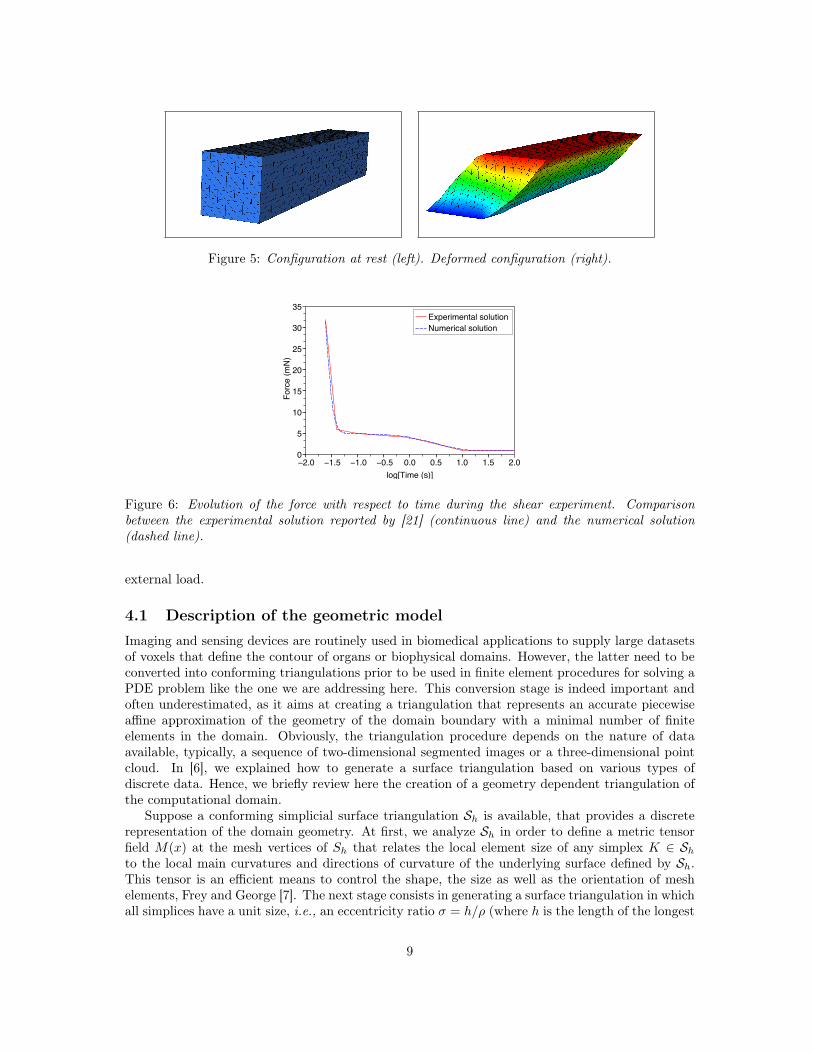
4.1 Description of the geometric modelImaging and sensing devices are routinely used in biomedical applications to supply large datasetsof voxels that define the contour of organs or biophysical domains. However, the latter need to beconverted into conforming triangulations prior to be used in finite element procedures for solving aPDE problem like the one we are addressing here. This conversion stage is indeed important andoften underestimated, as it aims at creating a triangulation that represents an accurate piecewiseaffine approximation of the geometry of the domain boundary with a minimal number of finiteelements in the domain. Obviously, the triangulation procedure depends on the nature of dataavailable, typically, a sequence of two-dimensional segmented images or a three-dimensional pointcloud. In [6], we explained how to generate a surface triangulation based on various types ofdiscrete data. Hence, we briefly review here the creation of a geometry dependent triangulation ofthe computational domain.

Suppose a conforming simplicial surface triangulation Sh is available, that provides a discreterepresentation of the domain geometry. At first, we analyze Sh in order to define a metric tensorfield M(x) at the mesh vertices of Sh that relates the local element size of any simplex K ∈ Shto the local main curvatures and directions of curvature of the underlying surface defined by Sh.This tensor is an efficient means to control the shape, the size as well as the orientation of meshelements, Frey and George [7]. The next stage consists in generating a surface triangulation in whichall simplices have a unit size, i.e., an eccentricity ratio σ = h/ρ (where h is the length of the longest

9

(a) (b)

(c) (d)

Figure 7: (a,b) Surface triangulation obtained from MRI slices. (c) Surface triangulation adaptedto the geometric properties. (d) Generation of a three-dimensional triangulation.

Figure 8: Computational mesh (left). Coronal cut through the computational mesh (right).

edge and ρ is the radius of the inscribed sphere) controlled by the tensor M(x). Figure 7 showsthe result of the surface retriangulation procedure on a biomedical model of a human head. The

10

next stage consists in creating a computational mesh Th of the domain suitable for finite elementscalculations. To this end, we rely on an efficient Delaunay point insertion procedure described in[7] that can be also used for adapting triangulations to any metric tensor given by an a posteriorierror estimate.

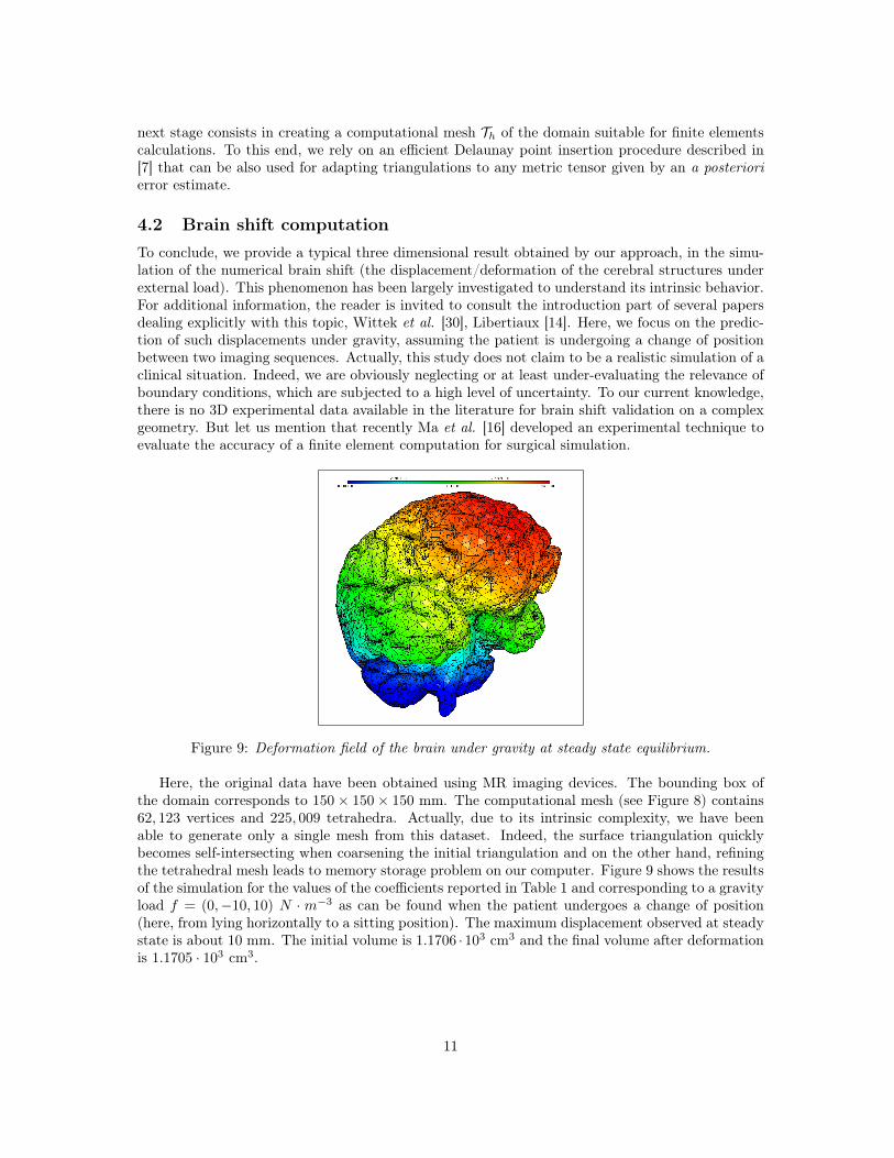
4.2 Brain shift computationTo conclude, we provide a typical three dimensional result obtained by our approach, in the simu-lation of the numerical brain shift (the displacement/deformation of the cerebral structures underexternal load). This phenomenon has been largely investigated to understand its intrinsic behavior.For additional information, the reader is invited to consult the introduction part of several papersdealing explicitly with this topic, Wittek et al. [30], Libertiaux [14]. Here, we focus on the predic-tion of such displacements under gravity, assuming the patient is undergoing a change of positionbetween two imaging sequences. Actually, this study does not claim to be a realistic simulation of aclinical situation. Indeed, we are obviously neglecting or at least under-evaluating the relevance ofboundary conditions, which are subjected to a high level of uncertainty. To our current knowledge,there is no 3D experimental data available in the literature for brain shift validation on a complexgeometry. But let us mention that recently Ma et al. [16] developed an experimental technique toevaluate the accuracy of a finite element computation for surgical simulation.

Figure 9: Deformation field of the brain under gravity at steady state equilibrium.

Here, the original data have been obtained using MR imaging devices. The bounding box ofthe domain corresponds to 150× 150× 150 mm. The computational mesh (see Figure 8) contains62, 123 vertices and 225, 009 tetrahedra. Actually, due to its intrinsic complexity, we have beenable to generate only a single mesh from this dataset. Indeed, the surface triangulation quicklybecomes self-intersecting when coarsening the initial triangulation and on the other hand, refiningthe tetrahedral mesh leads to memory storage problem on our computer. Figure 9 shows the resultsof the simulation for the values of the coefficients reported in Table 1 and corresponding to a gravityload f = (0,−10, 10) N · m−3 as can be found when the patient undergoes a change of position(here, from lying horizontally to a sitting position). The maximum displacement observed at steadystate is about 10 mm. The initial volume is 1.1706 ·103 cm3 and the final volume after deformationis 1.1705 · 103 cm3.

11

5 Conclusions and PerspectivesThis analysis has shown the ability of our generalized model to deal with a complex problem.However, it revealed the need to know biophysically meaningful coefficients, i.e. coming fromin vivo measurements, difficult to obtain in practice. To overcome this difficulty, we started toinvestigate a related inverse problem, in view of retrieving the biophysical coefficients in a fully noninvasive manner [5]. This study has to be considered as a preliminary stage of a more complex studyof the behavior of brain structures. The objective was not to devise the relevance of a viscoelasticmodel versus another type of model but to show our ability to perform numerical analysis and todeal with complex geometries. For this study to be meaningful, we are expecting collaborationswith biomechanicians that could be interested by the type of results presented here.

References[1] D.W.A. Brands, G.W.M. Peters, and P.H.M. Bovendeerd. Design and numerical implementa-

tion of a 3-D non-linear viscoelastic constitutive model for brain tissue during impact. Journalof Biomechanics, 37:127–134, 2004.

[2] M. Bucki, C. Lobos, and Y. Pahan. Bio-mechanical model of the brain for a per-operativeimage-guided neuronavigator compensating for brain-shift deformations. Computer Methodsin Biomechanics and Biomedical Engineering, Supplement 1:25–26, 2007.

[3] K. Darvish and J. Crandall. Nonlinear viscoelastic effects in oscillatory shear deformation ofbrain tissue. Medical Engineering & Physics, 23:633–645, 2001.

[4] M. de Buhan and P. Frey. A generalized model of nonlinear viscoelasticity : numerical issuesand applications. Int. J. Numer. Meth. Engng., 86:13:1049–1074, 2011.

[5] M. de Buhan and A. Osses. Logarithmic stability in determination of a 3D viscoelastic coeffi-cient and a numerical example. Inverse Problems, 26:095006, 2010.

[6] P. Frey. Generation and adaptation of computational surface meshes from discrete anatomicaldata. Int. J. Numer. Methods Eng., 60:1049–1074, 2004.

[7] P. Frey and P.-L. George. Mesh generation. Application to finite elements. Wiley, 2008.

[8] M. Hrapko, J.A.W. van Dommelen, G.W.M. Peters, and J.S.H.M. Wismans. The mechanicalbehaviour of brain tissue: Large strain response and constitutive modelling. Biorheology,43:633–636, 2006.

[9] C.E. Jamison, R.D. Marangoni, and A.A. Glaser. Viscoelastic properties of soft tissue bydiscrete model characterization. Journal of Biomechanics, 1:33–46, 1968.

[10] G. Joldes, A. Wittek, and K. Miller. Real-time nonlinear finite element computations on gpu??? application to neurosurgical simulation. Computer Methods in Applied Mechanics andEngineering, 199:3305 – 3314, 2010.

[11] G. Joldes, A. Wittek, and K. Miller. An adaptive dynamic relaxation method for solvingnonlinear finite element problems. application to brain shift estimation. International Journalfor Numerical Methods in Biomedical Engineering, 27(2):173–185, 2011.

[12] P. Le Tallec. Numerical methods for nonlinear three-dimensional elasticity. In Handbook ofNumerical Analysis, volume 3, pages 465–624. P. G. Ciarlet and J.L. Lions eds, North-Holland,1994.

12

[13] P. Le Tallec, C. Rahier, and A. Kaiss. Three-dimensional incompressible viscoelasticity in largestrains: formulation and numerical approximation. Computer methods in applied mechanicsand engineering, 109:233–258, 1993.

[14] V. Libertiaux. Contribution to the study of the mechanical properties of brain tissue: fractionalcalculus-based model and experimental characterization. Thèse de Doctorat de l’Université deLiège, 2010.

[15] J. Lubliner. A model of rubber viscoelasticity. Mechanics Research Communications, 12:93–99,1985.

[16] J. Ma, A. Wittek, S. Singh, G. Joldes, T. Washio, K. Chinzei, and K. Miller. Evaluation ofaccuracy of non-linear finite element computations for surgical simulation: study using brainphantom. Computer Methods in Biomechanics and Biomedical Engineering, 13(6):783–794,2010.

[17] M. I. Miga, K.D. Paulsen, F.E. Kennedy, P.J. Hoopes, A. Hartov, and D.W. Roberts. Modelingsurgical loads to account for subsurface tissue deformation during stereotactic surgery. IEEESPIE Proceedings of Laser-Tissue Interaction IX, Part B: Soft-tissue Modeling, 3254:501–511,1998.

[18] K. Miller. Constitutive modelling of brain tissue : experiment and theory. Journal of Biome-chanics, 30:1115–1121, 1997.

[19] K. Miller and K. Chinzei. Mechanical properties of brain tissue in extension. Journal ofBiomechanics, 35:483–490, 2002.

[20] K. Miller, K. Chinzei, G. Orssengo, and P. Bednarz. Mechanical properties of brain tissuein-vivo : experiment and computer simulation. Journal of Biomechanics, 33:1369–1376, 2000.

[21] X. Ning, Q. Zhu, Y. Lanir, and S.S. Margulies. A transversaly isotropic viscoelastic constitutiveequation for brainstem undergoing finite deformation. Journal of Biomechanical Engineering(ASME), 128:925–933, 2006.

[22] J. Nocedal and S.J. Wright. Numerical optimization. In Springer Series in Operations Research.Springer, 1999.

[23] J.T. Oden. Finite Elements for Nonlinear Continua. McGraw Hill, 1972.

[24] E. Pena, B. Calvo, M.A. Martinez, and M. Doblare. An anisotropic visco-hyperelastic modelfor ligaments at finite strains: formulation and computational aspects. International Journalof Solids and Structures, 44:760–778, 2007.

[25] P.P. Provenzano, R.S. Lakes, D.T. Corr, and R. Vanderby. Application of nonlinear viscoelasticmodels to describe ligament behaviour. Biomechanics and Modeling in Mechanobiology, 1:45–47, 2002.

[26] J.C. Simo. On a fully three-dimensional finite-strain viscoelastic damage model: formulationand computational aspects. Computer methods in applied mechanics and engineering, 60:153–173, 1987.

[27] K. Ueno, J. Melvin, L. Li, and J. Lighthall. Development of tissue level brain injury criteriaby finite element analysis. Journal of Neurotrauma, 12:695–706, 1995.

[28] A. Wittek, T. Hawkins, and K. Miller. On the unimportance of constitutive models in com-puting brain deformation for image-guided surgery. Biomech. Model Mechanobiol, 8:77–84,2009.

13

[29] A. Wittek, G. Joldes, and K. Miller. Algorithms for computational biomechanics of the brain.In Biomechanics of the Brain, Biological and Medical Physics, Biomedical Engineering, pages189–219. Springer New York, 2011.

[30] A. Wittek, R. Kikinis, S. Warfield, and K. Miller. Brain shift computation using a fullynonlinear biomechanical model. J. Duncan and G. Gerig Edition, pages 583–590, 2005.

14