A generalized recursive convolution method for time-domainpropagation in porous media

Didier Dragna,a) Pierre Pineau, and Philippe Blanc-BenonLaboratoire de M�ecanique des Fluides et d’Acoustique, Unit�e Mixte de Recherche, Centre National de laRecherche Scientifique 5509, �Ecole Centrale de Lyon, Universit�e de Lyon, 36, avenue Guy de Collongue,69134 �Ecully Cedex, France

(Received 2 December 2014; revised 3 April 2015; accepted 16 July 2015; published online 20August 2015)

An efficient numerical method, referred to as the auxiliary differential equation (ADE) method, is

proposed to compute convolutions between relaxation functions and acoustic variables arising in

sound propagation equations in porous media. For this purpose, the relaxation functions are

approximated in the frequency domain by rational functions. The time variation of the convolution

is thus governed by first-order differential equations which can be straightforwardly solved. The ac-

curacy of the method is first investigated and compared to that of recursive convolution methods. It

is shown that, while recursive convolution methods are first or second-order accurate in time, the

ADE method does not introduce any additional error. The ADE method is then applied for outdoor

sound propagation using the equations proposed by Wilson et al. in the ground [(2007). Appl.

Acoust. 68, 173–200]. A first one-dimensional case is performed showing that only five poles are

necessary to accurately approximate the relaxation functions for typical applications. Finally, the

ADE method is used to compute sound propagation in a three-dimensional geometry over an

absorbing ground. Results obtained with Wilson’s equations are compared to those obtained with

Zwikker and Kosten’s equations and with an impedance surface for different flow resistivities.VC 2015 Acoustical Society of America. [http://dx.doi.org/10.1121/1.4927553]

[VEO] Pages: 1030–1042

I. INTRODUCTION

Propagation of transient signals in porous media has im-

portant practical applications, for instance, in bioacoustics to

characterize bone properties (Cardoso et al., 2003; Fellah

et al., 2004; Ha€ıat et al., 2008), in building acoustics to

determine acoustic absorption of materials (Fellah et al.,2003) or in outdoor sound propagation to account for the

reflection of waves from the ground. For this type of signal,

time-domain methods are advantageous over frequency-

domain methods. The characterization of porous media in

the time domain is however not straightforward, as most of

the theoretical studies were conducted in the frequency

domain. For instance, the Biot’s equations for a viscous

fluid involve frequency-dependent parameters such as the

dynamic tortuosity, which lead in the time domain to convo-

lutions or to fractional derivatives [see, e.g., Fellah et al.(2013)]. In outdoor sound propagation, the solid frame can

be usually considered as not deformable (Attenborough

et al., 2011), and the behavior of porous media can be mod-

elled with the equivalent fluid approach using various mod-

els. The Zwikker and Kosten’s equations are usually chosen

in the literature (Salomons et al., 2002; Van Renterghem and

Botteldooren, 2003), as they are simple and easy to solve

numerically. However, it was shown that these equations

have limited applications as they are not well-suited for a

large range of grounds such as gravel, forests, or snow

(Wilson et al., 2007). Recently, more general time-domain

equations were proposed (Wilson et al., 2007; Umnova and

Turo, 2009). Unlike the Zwikker and Kosten’s equations,

they involve convolutions, which require storing the values

of the acoustic variables in the porous medium at all previ-

ous time steps in a naive approach. For a three-dimensional

(3D) geometry, a tremendous memory space is thus needed.

As a consequence, the use of these equations has been lim-

ited up to now to one- or two-dimensional geometries.

Therefore, an efficient numerical method is necessary to

evaluate convolutions with a reduced computational cost.

This problem has been thoroughly studied in electromag-

netic propagation as many real materials have frequency-

dependent properties. Three main methods emerged; all are

based on the approximation of frequency-dependent parame-

ters by a rational function in the frequency domain. The time-

domain counterpart corresponds to a sum of exponentially

decaying functions which permits a simplified computation

of the convolutions. In the first method, a time discretization

of the convolution is introduced. Assuming that the variables

are constant over one time step or vary linearly between two

consecutive time steps, the evaluation of the convolution can

be reduced to that of recursive expressions. Thus, the value of

the convolution at the actual time step depends on the one at

the previous time step only. These methods are called recur-

sive convolution methods (Luebbers and Hunsberger, 1992).

The second method uses the Z-transform formalism to discre-

tize in time the equations (Sullivan, 1992, 1996). As shown

by Sullivan (1996), the expressions obtained are very close to

those of the recursive convolution methods. In the third

method, originated from the work of Joseph et al. (1991), a

differentiation of the convolution is performed, yielding an

additional set of first-order differential equations, which area)Electronic mail: didier.dragna@ec-lyon.fr

1030 J. Acoust. Soc. Am. 138 (2), August 2015 0001-4966/2015/138(2)/1030/13/$30.00 VC 2015 Acoustical Society of America

solved using the same numerical techniques as employed for

the propagation equations. This method is referred to as the

auxiliary differential equations (ADE) method and can be

seen as a generalized recursive method as no additional

approximations on the time variations of the variables are

introduced.

There has already been some use of these convolution

methods in acoustics. To our knowledge, the first application

dates back to the work of Botteldooren (1997) which pro-

poses a recursive convolution method to account for the

effects of entropy and vorticity boundary layers on sound

propagation. Later, recursive convolution methods were

mainly employed to derive time-domain impedance bound-

ary conditions, for applications in duct acoustics (Reymen

et al., 2008; Li et al., 2012) and in outdoor sound propaga-

tion (Ostashev et al., 2007; Cott�e et al., 2009). An ADE

method was also proposed by Bin et al. (2009) for surface

impedance implementation. The Z-transform method has

received much less attention. It was used especially in duct

acoustics by €Ozy€or€uk and Long (1996) to derive a time-

domain impedance boundary condition in a presence of a

mean flow.

In addition, ADE methods are widely spread in geophy-

sics to include effects of anelastic materials from the work of

Day and Minster (1984). The impact of this paper is impor-

tant, as it was referred to as a main result in a reference book

on the subject (Carcione, 2001). Still for geophysics applica-

tions, the ADE method was used to compute propagation

into a viscoacoustic medium (Groby and Tsogka, 2006) in

which the pressure and the divergence of the displacement

are related by a frequency-dependent constant. More

recently, a diffusive representation for order 1/2 fractional

derivatives based on the same methodology was proposed to

study sound propagation in a porous medium using the Biot

theory for a particular model of dynamic permeability

(Blanc et al., 2013).

The main objectives of this paper are to compare the ac-

curacy of the ADE method to that of recursive convolution

methods and to apply the ADE method to sound propagation

in porous media. The feasibility of the approach is demon-

strated on a typical outdoor sound propagation problem in a

3D configuration.

The paper is organized as follows. In Sec. II, the ADE

method is described and the relation to the recursive convo-

lution methods is highlighted. The accuracy of these vari-

ous methods is then investigated. A first one-dimensional

test-case is performed to numerically retrieve the order of

accuracy derived analytically. In a second test-case, the

error introduced by the rational function approximation is

analyzed. Application of the ADE method to outdoor sound

propagation is performed in Sec. III. The time-domain

equations for Wilson’s relaxation model are solved in the

ground medium. A one-dimensional propagation calcula-

tion is first treated and the characteristics of the porous me-

dium are retrieved. Then, the feasibility of the method for

3D geometries is demonstrated by considering the propaga-

tion of a broadband impulse signal in an inhomogeneous

atmosphere.

II. RECURSIVE CONVOLUTION METHODS

A. ADE method

Time-domain equations in porous media usually involve

convolutions:

IðuðtÞ; tÞ ¼ ½u � s�ðtÞ ¼ðt

�1uðt0Þsðt� t0Þdt0; (1)

where s(t) is a real and causal function and is known a prioriand u(t) is an acoustic variable, generally the pressure or the

particle velocity. The function s(t) is typically a relaxation

function, describing the response of a porous medium to an

excitation and depends on the characteristics of the porous

medium. To efficiently compute the convolution, the Fourier

transform of the function s(t), defined by

sðxÞ ¼ðþ1�1

sðtÞeixtdt; (2)

is approximated by a rational function in �ix with simple

poles whose denominator and numerator are polynomials of

degree P:

s xð Þ � sP xð Þ ¼ s1 þa0 þ � � � þ aP�1 �ixð ÞP�1

1þ � � � þ bP �ixð ÞP; (3)

where s1 is the limit value of sðxÞ as x tends to infinity. As

s(t) is a real function, all the coefficients ai and bi are real,

and hence, the poles of sPðxÞ are either real, denoted here-

after by kk, or come in complex conjugate pairs, designated

by ak 6 ibk. For causality reasons, they are located in the

lower half x-plane, which imposes that kk� 0 and ak� 0.

Therefore, sPðxÞ can be rewritten as

sP xð Þ ¼ s1 þXN

k¼1

Ak

kk � ix

þXM

k¼1

1

2

Bk þ iCk

ak þ ibk � ixþ Bk � iCk

ak � ibk � ix

� �; (4)

with P¼Nþ 2M and where Ak, Bk, and Ck are numerical

parameters. In the time domain, the approximation is written

as

sðtÞ � s1dðtÞ þXN

k¼1

Ake�kktHðtÞ

þXM

k¼1

e�akt½Bk cosðbktÞ þ Ck sinðbktÞ�HðtÞ; (5)

where d(t) and H(t) stand for the Dirac and Heaviside func-

tions, respectively. A physical interpretation of each term

can be provided. As s1 is the high-frequency limit of sðxÞ,the first term corresponds to the instantaneous response to

the excitation. The second term is a classical relaxation

function which decays exponentially with time and whose

time constant is equal to 1/kk. Finally, the third term is an

J. Acoust. Soc. Am. 138 (2), August 2015 Dragna et al. 1031

oscillatory response damped with time. The period of oscil-

lations is governed by the imaginary part of the pole bk and

the decay with time by its real part ak. The approximation of

sðxÞ by a rational function can be obtained using various

numerical methods. Among them, the vector fitting method

proposed by Gustavsen and Semlyen (1999) is used

hereafter.

Introducing the approximation of s(t) given in Eq. (5)

into Eq. (1) leads to

IðuðtÞ; tÞ ¼ s1uðtÞ þXN

k¼1

Ak/kðtÞ

þXM

k¼1

½Bkwð1Þk ðtÞ þ Ckw

ð2Þk ðtÞ�; (6)

where the auxiliary functions /kðtÞ; wð1Þk ðtÞ, and wð2Þk ðtÞ, also

referred to as accumulators or memory variables in geophy-

sics, are given by the convolutions

/kðtÞ ¼ðt

�1uðt0Þe�kkðt�t0Þdt0; (7)

wð1Þk ðtÞ ¼ðt

�1uðt0Þe�akðt�t0Þ cosðbkðt� t0ÞÞdt0; (8)

wð2Þk ðtÞ ¼ðt

�1uðt0Þe�akðt�t0Þ sinðbkðt� t0ÞÞdt0: (9)

By differentiating Eqs. (7)–(9), it is straightforwardly deduced

that these auxiliary functions satisfy the following equations:

@/k

@tþ kk/k tð Þ ¼ u tð Þ; (10)

@w 1ð Þk

@tþ akw

1ð Þk tð Þ þ bkw

2ð Þk tð Þ ¼ u tð Þ; (11)

@w 2ð Þk

@tþ akw

2ð Þk tð Þ � bkw

1ð Þk tð Þ ¼ 0: (12)

This method is referred to as the ADE method because

additional first-order differential equations are solved using

standard numerical techniques, instead of computing directly

the convolutions and of storing the time evolution of the

variable u in the numerical domain.

B. Recursive convolution methods and relationto the ADE method

Recursive convolution methods are an alternative to the

ADE method. Instead of integrating first-order equations, the

time evolution of the auxiliary functions is obtained from re-

cursive expressions relating values at two consecutive time

steps. These expressions are obtained from those of the ADE

methods. Thus, the equation for /k in Eq. (10) is first written

in the form

@

@tekk t/k

� �¼ ekktu tð Þ: (13)

Then, discretizing in time the problem with an uniform time

step Dt and integrating over two consecutive time steps nDtand (nþ 1)Dt, with n an integer, lead to the relation

/k½ðnþ 1ÞDt� ¼ e�kkDt/k½nDt�

þ e�kkDt

ðDt

0

ekkt0u½tþ nDt�dt0: (14)

This formula is the basis of most recursive convolution

methods. Indeed, assuming that u(t) is constant in the inter-

val [nDt, (nþ 1)Dt] and is equal to u[(nþ 1)Dt] gives the

piecewise constant recursive convolution (PCRC) method

(Luebbers and Hunsberger, 1992):

/PCRCk nþ 1ð ÞDt½ � ¼ e�kkDt/PCRC

k nDt½ �

þ 1� e�kkDt

kku nþ 1ð ÞDt½ �: (15)

Similarly, the trapezoidal recursive convolution (TRC)

method (Siushansian and LoVetri, 1997) is obtained by

assuming that u(t) is constant in the interval [nDt, (nþ 1)Dt]and is equal to (u[nDt]þ u[(nþ 1)Dt])/2. Finally, in the

piecewise linear recursive convolution (PLRC) method

(Kelley and Luebbers, 1996), u is approximated by a linear

function in the interval [nDt, (nþ 1)Dt].Introducing wk ¼ wð1Þk þ iwð2Þk , a similar expression is

obtained from Eqs. (11) and (12) in the case of a complex

conjugate pair of poles:

wk½ðnþ 1ÞDt� ¼ e�ðakþibkÞDtwk½nDt�

þ e�ðakþibkÞDt

ðDt

0

eðakþibkÞt0u½tþ nDt�dt0:

(16)

C. Error introduced by recursive convolution methods

Unlike the ADE method, recursive convolution algo-

rithms introduce additional approximations on the variation

of u(t) during one time step. It is then interesting to deter-

mine the errors generated by these approximations. Thus,

one considers u(t) to be a time harmonic function, i.e.,

uðtÞ ¼ e�ixt. For the sake of simplicity, only real poles are

considered hereafter but the results can be extended straight-

forwardly to complex conjugate poles. In this case, from

Eq. (10), the auxiliary function /k is given by

/k tð Þ ¼ 1

kk � ixe�ixt: (17)

The analytical values of /k for the recursive convolution

methods can be obtained from the recursive formula in Eq.

(14). For example, the PCRC method leads for a harmonic

function u(t) to

/PCRCk tð Þ ¼ 1� e�kkDt

kke�ixt þ e�kkDt/PCRC

k t� Dtð Þ:

(18)

1032 J. Acoust. Soc. Am. 138 (2), August 2015 Dragna et al.

The auxiliary function /PCRCk can then be expressed as a

geometric series:

/PCRCk tð Þ ¼ 1� e�kkDt

kke�ixt

Xþ1n¼0

e �kkDtþixDtð Þn; (19)

which leads to the expression

/PCRCk tð Þ ¼ 1� e�kkDt

kke�ixt 1

1� e�kkDtþixDt: (20)

The auxiliary function in the PCRC approximation can then

be expressed as a function of the exact value of the auxiliary

function by

/PCRCk tð Þ ¼ /k tð Þ 1� e�kkDt

kkDt

kkDt� ixDt

1� e�kkDtþixDt: (21)

To determine the order of the approximation of the PCRC

method, a Taylor expansion in Dt of the preceding equation

is performed yielding

/PCRCk tð Þ ¼ /k tð Þ 1� ixDt

2þ O Dt2ð Þ

� �: (22)

This shows that the PCRC is only a first-order approxima-

tion. Therefore, when employing high-order time-integration

schemes, the use of the PCRC method is expected to deterio-

rate the accuracy. Similarly, for the TRC and PLRC meth-

ods, one gets the following estimates:

/TRCk tð Þ ¼ /k tð Þ 1þ kkDt

12ixDt� xDtð Þ2

12þ O Dt3ð Þ

" #;

(23)

/PLRCk tð Þ ¼ /k tð Þ 1� xDtð Þ2

12þ O Dt3ð Þ

" #: (24)

This shows that the TRC method is a second-order method,

as the error decreases as Dt2. The PLRC method is also a

second-order method and has a slightly better accuracy than

the TRC method.

D. Test-case

1. Accuracy of the recursive convolution algorithms

In this section, a test-case is performed to validate the

methods presented previously and to investigate their accu-

racy. For this purpose, one considers the equation

@p

@tþ c

@p

@xþ b1p� b1k/ ¼ 0; (25)

with b1 ¼ 0:01, c¼ 1, and k¼ 1 and

/ðtÞ ¼ðt

0

e�kðt�t0Þpðt0Þdt0: (26)

This corresponds to the advection equation

@p

@tþ c

@p

@xþ b � p ¼ 0; (27)

with an additional frequency-dependent dissipative term b(t)whose Fourier transform is given by

b xð Þ ¼ b1�ix

k� ix: (28)

At low frequencies, the dissipative term is almost zero while

at high frequencies, it tends to the constant value b1. The

frequency variation of bðxÞ between these two limits is gov-

erned by the parameter k. The initial disturbances are given

by

p x; t ¼ 0ð Þ ¼ 1� 2x2

B2

� �exp � x2

B2

� �; (29)

with B¼ 2.5 and the solution is advanced to t¼ 100. The

spatial differentiation is calculated using a Fourier pseudo-

spectral method [see, e.g., Boyd (2001)] to ensure a negligi-

ble error. The mesh size is Dx¼ 1. The time integration is

performed using a low storage fourth-order Runge-Kutta

algorithm (Berland et al., 2006). Using recursive convolu-

tion methods, the term �b1k/ in Eq. (25) is integrated in

first order according to time after updating the auxiliary

function /.

The time series of the solution at the initial and final

times are represented as a function of x in Fig. 1. The analyt-

ical solutions for / and p are given in Appendix A. The ini-

tial disturbances are symmetrical around x¼ 0 and the

maximum amplitude is equal to unity. At t¼ 100, the maxi-

mal amplitude is strongly reduced as it is equal to 0.6 due to

the dissipative term. Moreover, the shape of the time series

is modified as the solution is no longer symmetrical. This is

related to the frequency variations of bðxÞ. The numerical

solutions obtained at t¼ 100 for a time step Dt¼ 0.5 using

the PCRC and ADE methods are also represented in Fig.

1(b). It is seen that the numerical solution using the ADE

method is almost superimposed on the analytical solution,

while discrepancies are observed when using the PCRC

method. The curves obtained for the TRC and PLRC meth-

ods are not represented as they are similar to that obtained

for the ADE method.

A time-step convergence study is carried out to illustrate

the accuracy of the various methods. The error � on a quan-

tity of interest u is calculated with the formula

�½u� ¼ffiffiffiffiffiffiffiffiffiffiffiffiffiffiffiffiffiffiffiffiffiffiffiffiffiffiffiffiffiffiffiffiffiffiffiffiffiffiffiffiffiffiffiffiffiffiffiffiffiffiffiffiffiffiffiffiffiffiffiffiffiffiffiffiffiffiffiffiffiffiffiffiffiffiffiffið

D

juanaðx; t ¼ 100Þ � uðx; t ¼ 100Þj2dx

s; (30)

where uana is the analytical solution. The error on / is dis-

played in Fig. 2(a) as a function of the normalized time step

CFL¼ cDt/Dx, which corresponds to the Courant-Friedrichs-

Lewy number, for the different methods. The order of the

recursive convolution methods, obtained analytically in Sec.

II C is retrieved. Thus, the PCRC method is a first-order

method while the TRC and PLRC methods are second-order

accurate in time. Note also the error is smaller using the

J. Acoust. Soc. Am. 138 (2), August 2015 Dragna et al. 1033

PLRC method than the TRC method. In addition, the order of

accuracy of the ADE method corresponds to that of the time-

integration algorithm. In this case, as a fourth-order Runge-

Kutta scheme is used, it is seen that the ADE method is fourth-

order accurate. Concerning the error on p plotted as a function

of the normalized time step in Fig. 2(b), the accuracy of the so-

lution is strongly dependent on the accuracy of / and, in most

of the cases, the order of accuracy of p is that of /. Thus, using

the PCRC and ADE methods, p is first- and fourth-order accu-

rate in time, respectively. For the TRC and PLRC methods,

the solution is second-order accurate in time except for the

PLRC method with CFL smaller than 0.03, for which first-

order accuracy is observed. This behavior is related to the first-

order time-integration scheme used for the term �bk/.

2. Accuracy of the approximation by a rationalfunction

In this section, the influence of the approximation of a

relaxation function by a rational function on the accuracy is

investigated. With this aim, one considers the advection of

acoustic waves in a porous medium with an air flow resistiv-

ity r0, a tortuosity q, and porosity X, using one of the sim-

plest models, which is the Zwikker and Kosten’s model. In

the frequency-domain, the sound pressure is written as

@p

@x� ik xð Þp ¼ 0; (31)

where the acoustic wavenumber k(x) is given by (Salomons,

2001)

k xð Þ ¼ xq

c

ffiffiffiffiffiffiffiffiffiffiffiffiffiffiffiffiffi1þ x0

�ix

r; (32)

with x0 ¼ r0X=ðq0q2Þ. Multiplying both sides of Eq. (31)

byffiffiffiffiffiffiffiffiffiffiffiffiffiffiffiffiffiffiffiffiffiffiffiffiffiffiffiffiffi1þ x0=ð�ixÞ

pleads to

�ixp þ c

q

ffiffiffiffiffiffiffiffiffiffiffiffiffiffiffiffiffi1þ x0

�ix

r@p

@xþ x0p ¼ 0; (33)

which is written back in the time domain as

@p

@tþ c

qs � @p

@x

� �þ x0p ¼ 0; (34)

where the relaxation function s(t) is the inverse Fourier

transform of

s xð Þ ¼ffiffiffiffiffiffiffiffiffiffiffiffiffiffiffiffiffi1þ x0

�ix

r: (35)

FIG. 1. Time series of p (a) at the initial time and (b) at the final time

t¼ 100 as a function of x: (black solid line) analytical solution and numeri-

cal solutions using (black dashed line) the PCRC method and (gray dashed

line) the ADE method.

FIG. 2. Error on (a) / and (b) p as a function of the normalized time step

CFL¼ cDt/Dx using (thin dashed line) the PCRC method, (thick dashed

line) the TRC method, (solid line) the PLRC method, and (dashed-dotted

line) the ADE method.

1034 J. Acoust. Soc. Am. 138 (2), August 2015 Dragna et al.

The parameter x0 is a characteristic of the medium which

separates two regimes. For x� x0, the advection equation

can be written as a diffusion equation:

@p

@t� D

@2p

@x2¼ 0; (36)

with a diffusivity coefficient D ¼ c2=ðq2x0Þ. For x x0,

the advection equation has the simple form

@p

@tþ c

q

@p

@xþ x0p ¼ 0; (37)

whose solutions are evanescent waves which propagated at a

sound speed c/q and whose damping is related to x0.

As in the previous test-case, a Fourier pseudospectral

method is used. The characteristics of the porous medium

are set to r0¼ 10 kPA s m�2, q¼ 1.8, and X¼ 0.5. The mesh

size is uniform with Dx¼ 0.0085 m. The initial perturbations

are given by

p x; t ¼ 0ð Þ ¼ C cos2px

A

� �exp � x2

B2

� �; (38)

with C¼ 1 Pa, A¼ 4Dx, and B¼ 6Dx. The solution is

advanced up to t¼ 0.003 s. The time step is set to 2.5 10�5 s

and the CFL number CFL¼ c0Dt/Dx is equal to one. The

ADE method is used to handle the convolution. Therefore,

instead of considering Eq. (34), the following first-order

equations are solved:

@p

@tþ c

q

@p

@xþ c

q

XN

k¼1

Ak/k þ x0p ¼ 0; (39)

@/k

@tþ kk/k ¼

@p

@x; (40)

where a rational function with real poles only is used to ap-

proximate sðxÞ:

s xð Þ � sN xð Þ ¼ 1þXN

k¼1

Ak

kk � ix: (41)

The vector fitting algorithm is employed to get the coeffi-

cients Ak and kk and is initialized using a vector of 100 loga-

rithmically spaced frequencies fi between 50 Hz and 20 kHz.

The number of poles N is chosen between 1 and 10. The rela-

tive error over the whole frequency band of interest, com-

puted with

�½s� ¼X100

i¼1

ðsðxiÞ � sNðxiÞÞ2X100

i¼1

ðsðxiÞ � 1Þ2; (42)

is represented as a function of N on a logarithmic scale along

the vertical axis in Fig. 3. It is observed that the error

decreases exponentially with the number of poles. Thus, the

approximation error is large using only one pole, about

21.1% but is greatly reduced as N increases. Therefore, it is

equal to 3.82% for N¼ 2 and to 0.7% only for N¼ 3.

The solutions obtained from both the analytical solution

given in Appendix B and the numerical solutions at the final

time for various number of poles in the rational function

approximation are represented as a function of x in Fig. 4.

The amplitude of the numerical solution obtained by neglect-

ing the convolution, which corresponds to the case N¼ 0, is

smaller than that of the analytical solution. Thus, the maximal

amplitude is 0.15 Pa for the analytical solution and only

0.03 Pa for the numerical solution. This shows that the convo-

lution term has a strong influence on the numerical solution.

Using only one pole for the recursive convolution method

allows one to reduce the discrepancies as the maximal ampli-

tude for the numerical solution is now 0.12 Pa. For N� 2, the

amplitude obtained analytically is retrieved and the analytical

and numerical solutions are almost superimposed.

As done in Sec. II D 1, a time-step convergence analysis

is performed. The error is computed at the final time

t¼ 0.003 s, using Eq. (30). It is plotted as a function of the

normalized time step CFL¼ cDt/Dx in Fig. 5 for various

numbers of poles. For small values of N, i.e., N¼ 0 and

N¼ 1, the error does not depend on the time step. It is mostly

generated by the omission of the convolution for N¼ 0 or by

the inaccurate approximation of the relaxation function by a

FIG. 3. Error on the relaxation function as a function of the number of

poles.

FIG. 4. Time series of p for (gray dashed line) the analytical solution and

for the numerical solution (black dashed-dotted line) without the convolu-

tion term and with the convolution term with (black dashed line) one pole

and (black solid line) two poles.

J. Acoust. Soc. Am. 138 (2), August 2015 Dragna et al. 1035

rational function with only one pole for N¼ 1. Therefore,

reducing the time step does not allow us to reduce the error

in these cases. For larger values of N, which are N¼ 2, 3, 4

and 6, the variations of the error with the CFL present simi-

lar shapes. For large CFL, the error decreases as (Dt)4, which

is expected as a fourth-order time-integration algorithm is

used. As the CFL is reduced, the error reaches a plateau, and

does not depend anymore of the CFL but only on the number

of poles. For instance, it is equal to 7 10�4 for N¼ 2 and is

reduced to 5 10�5, 4 10�6, and 1.6 10�8 for N¼ 3, 4,

and 6, respectively. For N sufficiently large, N> 10 in this

case, the error curve is a straight line. Indeed, the rational

function approximation of the relaxation function is accurate

enough so that the error is mainly generated by the time-

integration method.

III. APPLICATION TO OUTDOOR SOUNDPROPAGATION

In this section, the ADE method is employed for study-

ing sound propagation in an inhomogeneous atmosphere.

A. Numerical aspects

1. Equations

In the air, a set of coupled equations for the acoustic

pressure p and acoustic particle velocity v accounting for a

mean flow V0 are solved (Ostashev et al., 2005). They corre-

spond to the linearized Euler equations with the omission of

terms of order ðjV0j=cÞ2. In the porous medium, the time-

domain equations for the Wilson’s relaxation model are

solved. They are given by (Wilson et al., 2007)

@v

@tþ X

q0q2sv � rp½ � þ 1

svv ¼ 0; (43)

@p

@tþ q0c2

Xse � r � vð Þ½ � ¼ 0; (44)

where the functions sv and se,

sv ¼ d tð Þ � 1

2s

t

sv; 1

� �; (45)

se ¼ d tð Þ � c� 1

cs

t

se; c� 1

� �; (46)

describe the viscous and thermal diffusion processes in the

porous medium, with characteristic relaxation times sv and

se, respectively. They are related to the characteristics of the

medium with sv ¼ 2q0q2=ðXr0Þ and se ¼ Prs2Bsv (Wilson

et al., 2007), where Pr is the Prandtl number and sB is a pore

shape factor set to one hereafter. The function s(t/s, a) in

Eqs. (45) and (46) is a general relaxation function such as its

Fourier transform sðxs; aÞ is written as

s xs; að Þ ¼1þ affiffiffiffiffiffiffiffiffiffiffiffiffiffiffiffi

1� ixsp

þ a: (47)

Applying the ADE method to the Wilson’s equations

lead to the resolution of the set of four equations:

@v

@tþ X

q0q2rpþ X

q0q2

XNv

k¼1

Avk/vk þ

1

svv ¼ 0; (48)

@p

@tþ q0c2

Xr � vþ q0c2

X

XNe

k¼1

Aek/

ek ¼ 0; (49)

@/vk@tþ kv

k/vk ¼ rp; (50)

@/ek

@tþ ke

k/ek ¼ r � v; (51)

where the relaxation functions have been approximated

using real poles only:

sv xð Þ � 1þXNv

k¼1

Avk

kvk � ix

; (52)

se xð Þ � 1þXNe

k¼1

Aek

kek � ix

: (53)

2. Numerical techniques

The Fourier pseudospectral method offers advantages

compared to finite difference methods, as spatial derivatives

are accurately evaluated using only two points per wave-

length. However, it requires the solution to be periodic in

space and smooth. The accuracy of the Fourier pseudospec-

tral method is therefore seriously degraded by the presence

of discontinuities. An extended Fourier pseudospectral

method was recently proposed to handle fluid media with

piecewise homogeneous properties (Hornikx et al., 2010)

but cannot be applied to our case, as the porous medium

properties are frequency-dependent and can also vary in

space. Therefore, the spatial derivatives in the direction per-

pendicular to the interface between the air and the porous

medium are evaluated using optimized fourth-order finite

FIG. 5. Error on p as a function of the normalized time step CFL¼ c0Dt/Dxfor various numbers of poles: (black thin dashed line) N¼ 0, (black thin

dashed-dotted line) N¼ 1, (black thin solid line) N¼ 2, (black thick dashed

line) N¼ 3, (black thick dashed-dotted line) N¼ 4, (black thick solid line)

N¼ 6, and (gray thick solid line) N¼ 10.

1036 J. Acoust. Soc. Am. 138 (2), August 2015 Dragna et al.

difference schemes (Bogey and Bailly, 2004) previously

employed in outdoor sound propagation studies (Dragna

et al., 2011, 2013). These schemes allow us to calculate

acoustic wavelength down to five or six points per wave-

length. In the directions parallel to the ground interface, the

Fourier pseudospectral method is used.

As the equations governing sound propagation in the air

and in the porous medium are different, the numerical do-

main is split into two subdomains, one for the air and one for

the porous medium. At the interface between the two subdo-

mains, a patching technique based on the characteristic vari-

ables [as described, for instance, in Hornikx (2009)] is

employed. It is detailed in Appendix C. At the outer bounda-

ries, perfectly matched layers in the split version as in

Hornikx et al. (2010) are used.

B. One-dimensional test case

A one-dimensional test-case is first performed. The pa-

rameters of the porous medium are set to r0¼ 10 kPa s m�2,

q¼ 1.8, and X¼ 0.5. The two relaxation functions are

approximated using 5 real poles on the frequency band

between 50 Hz and 20 kHz. In addition to the acoustic pres-

sure and velocity, there are thus for a one-dimensional test-

case ten supplementary variables in the porous medium to

store. Compared to a direct evaluation of convolutions or to

more sophisticated methods, the recursive convolution meth-

ods allows one to save a very large memory space and also

computational time. For instance, for the same case and for a

frequency of 800 Hz, Wilson et al. (2007) need 800 addi-

tional terms for evaluating each convolution. Increasing the

frequency would even require to store more and more terms.

The porous and air media are located at x< 0 and x> 0,

respectively. The mesh grid in the porous and air media

is uniform and the corresponding spatial steps are Dxp

¼ 0.0014 m and Dxa¼ 0.0028 m, respectively. In the air do-

main, this corresponds to a minimum of six points per wave-

length, which is necessary for accuracy, as indicated in the

preceding paragraph. The mesh size in the porous medium is

smaller, as the non-centered finite-difference schemes used

at the interface are quite dissipative for small wavelengths

and add a significant attenuation to that due to the porous

medium. As shown later, a resolution of 12 points per wave-

length is sufficient so that the numerical attenuation of the

signal in the porous medium corresponds to the theoretical

attenuation. There are 1000 and 1225 points in the air and in

the porous medium, respectively. The CFL number is set to

unity. An impulse source similar to that in Eq. (29) is used

with B¼ 3Dxa, and is located initially at xS¼ 1 m.

To validate the implementation of the Wilson’s relaxa-

tion equations, the characteristic impedance of the medium

is computed and compared to the analytical expression:

ZW ¼qq0c0

X1þ c� 1ffiffiffiffiffiffiffiffiffiffiffiffiffiffiffiffiffi

1� ixse

p� �

1� 1ffiffiffiffiffiffiffiffiffiffiffiffiffiffiffiffiffi1� ixsvp

� �� ��1=2

:

(54)

Thus, a Fourier transform of the acoustic pressure and veloc-

ity, denoted by p and v, at a node located at x¼�0.25 m is

performed. The characteristic impedance Z is then obtained

by computing the ratio between these two quantities, i.e.,

Z ¼ �p=v. The minus sign is necessary as the wave propa-

gates toward negative x. The real and imaginary parts of Zare represented as a function of the frequency along with

those of the analytical expression in Fig. 6. A good accord-

ance is obtained over the whole frequency band of interest.

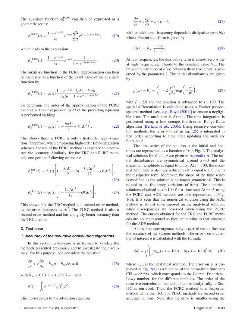
A further validation is performed by comparing the

attenuation of the signal inside the porous medium. As pro-

posed in Wilson et al. (2007), the attenuation is computed at

two consecutive grid nodes in the porous medium with

a ¼ log½pðx; xþ DxÞ=pðx; xÞ�=Dx. It is plotted as a function

of the frequency in Fig. 7. The analytical expression of

a¼ Im[kW], with

kW ¼qxc0

1þ c� 1ffiffiffiffiffiffiffiffiffiffiffiffiffiffiffiffiffi1� ixse

p� �

1� 1ffiffiffiffiffiffiffiffiffiffiffiffiffiffiffiffiffi1� ixsvp

� �" #1=2

;

(55)

is also represented in Fig. 7. The agreement between the nu-

merical and analytical solutions is satisfactory up to the max-

imal frequency of interest.

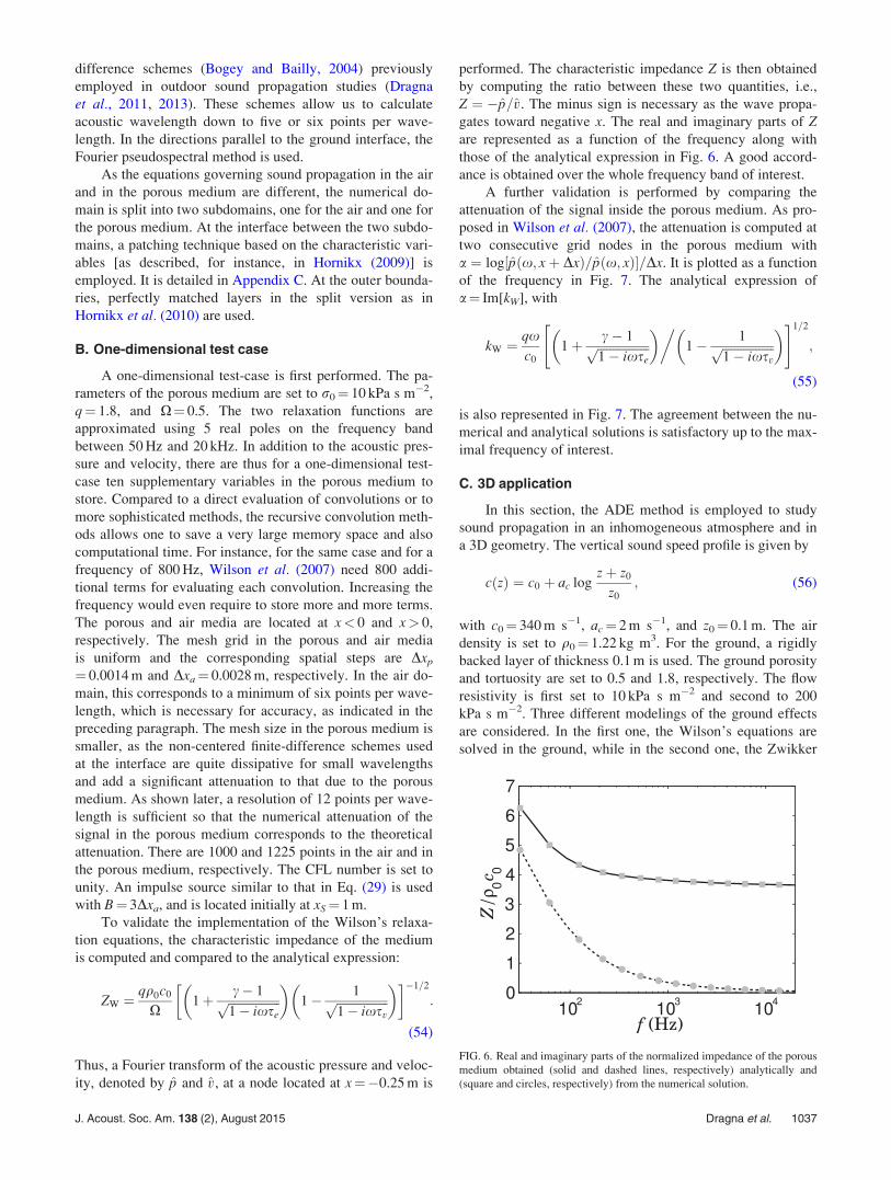
C. 3D application

In this section, the ADE method is employed to study

sound propagation in an inhomogeneous atmosphere and in

a 3D geometry. The vertical sound speed profile is given by

c zð Þ ¼ c0 þ ac logzþ z0

z0

; (56)

with c0¼ 340 m s�1, ac¼ 2 m s�1, and z0¼ 0.1 m. The air

density is set to q0¼ 1.22 kg m3. For the ground, a rigidly

backed layer of thickness 0.1 m is used. The ground porosity

and tortuosity are set to 0.5 and 1.8, respectively. The flow

resistivity is first set to 10 kPa s m�2 and second to 200

kPa s m�2. Three different modelings of the ground effects

are considered. In the first one, the Wilson’s equations are

solved in the ground, while in the second one, the Zwikker

FIG. 6. Real and imaginary parts of the normalized impedance of the porous

medium obtained (solid and dashed lines, respectively) analytically and

(square and circles, respectively) from the numerical solution.

J. Acoust. Soc. Am. 138 (2), August 2015 Dragna et al. 1037

and Kosten’s equations are employed. In the third one, the

propagation of acoustic waves in the ground is not modelled

and surface impedance corresponding to the Wilson relaxa-

tion model of a rigidly backed layer is used. This is done

employing a time-domain impedance boundary condition

presented in Cott�e et al. (2009) and Dragna et al. (2013). For

configurations where propagation equations in the ground

are solved, the grid has 1536 128 734 points which cor-

responds to a total of more than 144 106 of points. The

spatial step is Dx¼Dy¼ 0.1 m in the x- and y-directions

along which the Fourier pseudospectral method is used. In

the z-direction, finite difference schemes are employed with

a reduced accuracy and the spatial step is diminished to

Dza¼ 0.035 m in the air and to Dzp¼ 0.008 m in the porous

medium. A schematic of the grid in the x-z plane is repre-

sented in Fig. 8. For configurations using the impedance

boundary condition, the grid is similar except that the porous

medium is not modelled. The time step is chosen as

2.45 10�5 s. The simulation is initialized by setting

vðt ¼ 0Þ ¼ 0; (57)

p t ¼ 0ð Þ ¼ q0c20 exp �

x2 þ y2 þ z� zSð Þ2

B2

� �; (58)

with B¼ 0.24 m and where the height of the source is

zS¼ 1 m. The simulations are run up to t¼ 0.47 s. It is

worthwhile noting that the increase in memory space due to

the addition of the auxiliary functions for computing the con-

volutions is only 4% in this case.

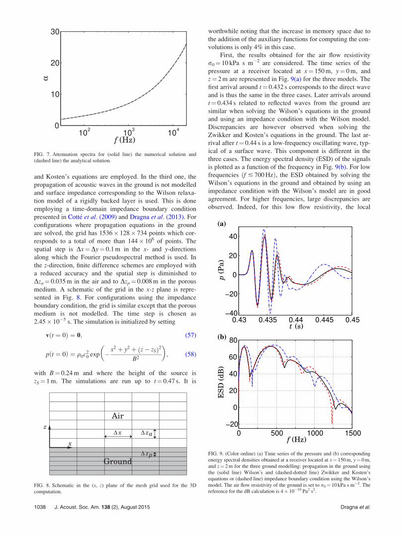
First, the results obtained for the air flow resistivity

r0¼ 10 kPa s m�2 are considered. The time series of the

pressure at a receiver located at x¼ 150 m, y¼ 0 m, and

z¼ 2 m are represented in Fig. 9(a) for the three models. The

first arrival around t¼ 0.432 s corresponds to the direct wave

and is thus the same in the three cases. Later arrivals around

t¼ 0.434 s related to reflected waves from the ground are

similar when solving the Wilson’s equations in the ground

and using an impedance condition with the Wilson model.

Discrepancies are however observed when solving the

Zwikker and Kosten’s equations in the ground. The last ar-

rival after t¼ 0.44 s is a low-frequency oscillating wave, typ-

ical of a surface wave. This component is different in the

three cases. The energy spectral density (ESD) of the signals

is plotted as a function of the frequency in Fig. 9(b). For low

frequencies ðf � 700 HzÞ, the ESD obtained by solving the

Wilson’s equations in the ground and obtained by using an

impedance condition with the Wilson’s model are in good

agreement. For higher frequencies, large discrepancies are

observed. Indeed, for this low flow resistivity, the local

FIG. 7. Attenuation spectra for (solid line) the numerical solution and

(dashed line) the analytical solution.

FIG. 8. Schematic in the (x, z) plane of the mesh grid used for the 3D

computation.

FIG. 9. (Color online) (a) Time series of the pressure and (b) corresponding

energy spectral densities obtained at a receiver located at x¼ 150 m, y¼ 0 m,

and z¼ 2 m for the three ground modelling: propagation in the ground using

the (solid line) Wilson’s and (dashed-dotted line) Zwikker and Kosten’s

equations or (dashed line) impedance boundary condition using the Wilson’s

model. The air flow resistivity of the ground is set to r0¼ 10 kPa s m�2. The

reference for the dB calculation is 4 10�10 Pa2 s2.

1038 J. Acoust. Soc. Am. 138 (2), August 2015 Dragna et al.

reaction assumption is expected to be not valid. Concerning

the ESD obtained with the Zwikker and Kosten’s equations,

it is seen that the results are dramatically different to that

obtained with the Wilson’s equations. For instance, the loca-

tion of the interferences is shifted. The first interference dip

is at a frequency of 150 Hz using the Wilson’s equations and

at a frequency of 180 Hz using the Zwikker and Kosten’s

equations. As discussed in Wilson et al., the Zwikker and

Kosten’s equations are not adapted for grounds with a low

flow resistivity and should not be used in these cases.

Finally, the results obtained for a ground with an air

flow resistivity r0¼ 200 kPa s m–2 are examined. The time

series of the pressure are shown in Fig. 10(a). The wave-

forms obtained by solving the Wilson’s equations in the

ground and obtained by using an impedance condition with

the Wilson’s model are almost superimposed. Moreover,

some small discrepancies can be observed on the waveform

obtained with the Zwikker and Kosten’s equations, espe-

cially around t¼ 0.436 s. Concerning the ESD of the signal

plotted as a function of the frequency in Fig. 10(b), it is

observed that the ESD is the same when solving the

Wilson’s equations and using an equivalent impedance

boundary condition. Indeed, the ground is hard enough so

that the local reaction assumption is valid. The ESD obtained

for the Zwikker and Kosten’s equations is also not too far

from that obtained with the Wilson’s equations. It is

retrieved that the Zwikker and Kosten’s equations are valid

for propagation over a grassy soil.

IV. CONCLUSION

Time-domain equations in porous media usually involve

convolutions between relaxation functions and acoustic vari-

ables, which are not straightforward to compute. A method,

referred to as the ADE method and originated from the elec-

tromagnetism and geophysics communities, was proposed to

efficiently evaluate these convolutions. For this purpose, the

relaxation functions are approximated by rational functions

in the frequency domain. The convolution is replaced by a

sum of new variables, called the auxiliary functions, whose

time variations are governed by first-order partial differential

equations. The accuracy of the ADE method was first inves-

tigated and compared to recursive convolution methods. It

was shown that recursive methods are low order methods,

while the ADE method does not modify the order of the

time-integration scheme. Therefore, the ADE method is

well-suited when employing high-order numerical schemes.

The influence of the number of poles for the approximation

of the relaxation function was then examined, showing that a

few number of poles is typically sufficient to have accurate

results. At last, the ADE method was applied to outdoor

sound propagation using the equations of the Wilson’s relax-

ation model to compute the propagation into the ground.

A one-dimensional test-case was first considered to demon-

strate the feasibility and the efficiency of the method. In

particular, the computed characteristic impedance and

attenuation in the ground were successfully compared to the

analytical values. An application of the method to a 3D prob-

lem was then performed for two different types of ground

and results were compared to those obtained using an equiv-

alent impedance boundary condition or solving the Zwikker

and Kosten’s equations in the ground. For a very soft

ground, the results substantially differ, in particular, close to

the ground for the surface wave component. For a harder

ground, the results obtained using the impedance boundary

condition and the Wilson’s relaxation equations in the

ground are in close agreement while those obtained employ-

ing the Zwikker and Kosten’s equations in the ground still

slightly differ.

ACKNOWLEDGMENTS

This work was granted access to the HPC resources of

IDRIS under the allocation 2014-022203 made by GENCI

(Grand Equipement National de Calcul Intensif). It was

performed within the framework of the Labex CeLyA of

Universit�e de Lyon, operated by the French National

Research Agency (ANR-10-LABX-0060/ANR-11-IDEX-

0007).

FIG. 10. (Color online) (a) Time series of the pressure and (b) corresponding

energy spectral densities obtained at a receiver located at x¼ 150 m, y¼ 0 m,

and z¼ 2 m for the three ground modelling: propagation in the ground using

the (solid line) Wilson’s and (dashed-dotted line) Zwikker and Kosten’s equa-

tions, or (dashed line) impedance boundary condition using the Wilson’s

model. The air flow resistivity of the ground is set to r0¼ 200 kPa s m�2.

The reference for the dB calculation is 4 10�10 Pa2 s2.

J. Acoust. Soc. Am. 138 (2), August 2015 Dragna et al. 1039

APPENDIX A: ANALYTICAL SOLUTION FOR THEINITIAL VALUE PROBLEM IN SEC. II

An analytical solution for the initial value problem pro-

posed in Sec. II D 1 is here given. The equation is

@p

@tþ c

@p

@xþ b1p� b1k/ ¼ 0; (A1)

with the initial value p(x, t¼ 0)¼Q(x) and with /ðx; t޼Рt

0e�kðt�t0Þpðx; t0Þdt0. Multiplying all terms by ekt, the pre-

ceding equation can be rewritten as

ekt @p

@tþ cekt @p

@xþ b1ektp� b1k

ðt

0

ekt0p t0ð Þdt0 ¼ 0:

(A2)

By derivating the equation and removing the factor ekt, one

obtains

@2p

@t2þ kþ b1 � @p

@tþ c

@2p

@x@tþ ck

@p

@x¼ 0: (A3)

Introducing the spatial Fourier transform

~pðk; tÞ ¼ð1�1

pðx; tÞe�ikxdx; (A4)

Eq. (A3) becomes

@2~p

@t2þ kþ b1 þ ikc � @~p

@tþ ikck~p ¼ 0: (A5)

Using the initial conditions

~p k; t ¼ 0ð Þ ¼ ~Q kð Þ; @~p

@tk; t ¼ 0ð Þ ¼ � ikcþ b1

�~Q kð Þ;

(A6)

where ~QðkÞ is the Fourier transform of Q(x), the solution is

p x; tð Þ ¼1

2p

ð1�1

~Q Aþ exp xþtð Þ þ A� exp x�tð Þ� �

eikxdk;

(A7)

with

x6 ¼1

2�k� b1 � ikc6

ffiffiffiffiffiffiffiffiffiffiffiffiffiffiffiffiffiffiffiffiffiffiffiffiffiffiffiffiffiffiffiffiffiffiffiffiffiffiffiffiffiffiffiffiffiffiffiffikþ b1 þ ikc �2 � 4ikck

q� �;

(A8)

A6 ¼x7 þ ikcþ b1

x6 � x7

: (A9)

Using Eq. (13), the analytical solution for / is straightfor-

wardly deduced, yielding

/ x; tð Þ ¼1

2p

ð1�1

~QAþ

xþ þ kexp xþtð Þ

�

þ A�x� þ k

exp x�tð Þ�

eikxdk: (A10)

APPENDIX B: ANALYTICAL SOLUTION FOR THEZWIKKER AND KOSTEN ADVECTION EQUATION

An analytical solution is proposed for the Zwikker and

Kosten’s advection equation:

@p

@tþ c

q

@p

@xþ c

qs � @p

@x

� �þ x0p ¼ 0; (B1)

with p(x, t¼ 0)¼Q(x). Introducing the Fourier-Laplace

transform

�pðk;xÞ ¼ðþ1

0

ðþ1�1

pðx; tÞeixt�ikxdx dt; (B2)

Eq. (B1) becomes

�p k;xð Þ ¼~Q kð Þ

D x; kð Þ ; (B3)

where ~QðkÞ is the Fourier transform of Q(x) and D(x, k) is

the dispersion equation

D x; kð Þ ¼ x0 � ixþ ikc

q

ffiffiffiffiffiffiffiffiffiffiffiffiffiffiffiffiffi1þ x0

�ix

r: (B4)

The branch cut of the square root function is chosen as the

negative real axis, so that the branch cut corresponds in

the x-plane to the line segment Re[x]¼ 0 and Im[x]

2 [�x0, 0]. The dispersion equation has two zeros both

located in the lower half x-plane. The first one is located at

�ix0 and is not of interest here. The second one, denoted

by xþ is purely imaginary if jkjc=q < x0=2 and is located

on the branch-cut at

xþ ¼ �ix0

2þ i

ffiffiffiffiffiffiffiffiffiffiffiffiffiffiffiffiffiffiffiffix2

0

4� k2c2

q2

s: (B5)

If jkjc=q > x0=2, it is located on the lower half-plane at

xþ ¼ �ix0

2þ kc

q

ffiffiffiffiffiffiffiffiffiffiffiffiffiffiffiffiffiffiffi1� x2

0q2

4c2k2

r: (B6)

The pressure in the time-domain can then be obtained

by the transform

p x; tð Þ ¼1

4p2

ðþ1�1

ðþ1�1

�p k;xð Þe�ixtþikxdx dk: (B7)

The x-integral can first be evaluated using the contour repre-

sented in Fig. 11. The acoustic field is a sum of two contribu-

tions p¼ pbcþ pþ. The term pbc is the contribution of the

branch cut

pbc x; tð Þ ¼1

4p2

ðþ1�1

~pbc k; tð Þeikxdk; (B8)

with

1040 J. Acoust. Soc. Am. 138 (2), August 2015 Dragna et al.

~pbc k; tð Þ ¼ð�ix0þ�

�

~Q kð ÞD x; kð Þ dxþ

�ix0��

~Q kð ÞD x; kð Þ dx;

(B9)

where �> 0 is a small parameter. As � tends to 0, the last

equation can be rewritten as

~pbc k; tð Þ¼� ~Q kð Þð1

0

e�x0vt

ffiffiffivpffiffiffiffiffiffiffiffiffiffi1� vp 2ikcqx0

q2x2 1� vð Þv� k2c2dv:

(B10)

It represents a stationary wave which decays exponentially

with time. The second contribution to the acoustic field pþ is

a propagating wave, which is obtained from the zero of the

dispersion equation, yielding

pþ x; tð Þ ¼1

2p

ðþ1�1

�2ixþ ~Q kð Þx0� 2ixþ

e�ixþteikxHjkjcq�x0

2

� �dk:

(B11)

APPENDIX C: PATCHING TECHNIQUES

The patching techniques used to transmit information

through the two subdomains, corresponding to the air and to

the porous medium, are described in the case of Wilson’s

equations. For this purpose, the characteristic variables are

determined from the equations in Eqs. (48)–(51) after having

introduced the ADE equations. These equations are rewritten

in the form

@U

@tþ A

@U

@xþ B

@U

@yþ C

@U

@zþ DU ¼ 0; (C1)

where U is the vector of unknown variables:

U ¼ ½v p /vk /ek�

T : (C2)

Without loss of generality, one considers two media whose

interface is located along the x axis at x¼ 0. The characteris-

tic variables are obtained by diagonalizing the matrix

A ¼ PKP�1, where K is a diagonal matrix whose diagonal

contains all the eigenvalues of A and P is a matrix whose

columns are the corresponding eigenvectors. For a 3D geom-

etry, the eigenvalues of the matrix A are c/q, �c/q, and 0,

which is repeated 2þ 3NvþNe times. Equation (C1) can

thus be rewritten as

@ ~U

@tþ K

@ ~U

@xþ S ¼ 0; (C3)

where ~U ¼ P�1U is the vector of characteristic variables and

S is a matrix which depend on ~U; @=@y, and @/@z but does

not depend on @/@x. Therefore, the characteristic variables

u! and u , associated to the eigenvalues c/q and �c/qrepresent outgoing and incoming waves traveling along the

x-direction, respectively. Simple algebraic manipulations

show that they are given by

u ¼ p� q0cq

Xvx; (C4)

u! ¼ pþ q0cq

Xvx: (C5)

The other characteristic variables associated to the eigen-

value 0 do not propagate in the x-direction. Note that the

characteristic variables for the Zwikker and Kosten’s equa-

tions have the same expressions.

Therefore, at the interface of the two media with differ-

ent properties, the outgoing characteristic variable u!1 in me-

dium 1 located at x< 0 and the incoming characteristic

variable u 2 in medium 2 located at x> 0 are computed at

each step of the Runge-Kutta algorithm. Imposing the conti-

nuity of the pressure and normal velocity at the interface, the

acoustic variables are thus updated using the characteristic

variables. For instance, if the medium 1 is a porous medium

with a tortuosity q and a porosity X and if the medium 2 cor-

responds to air, the pressure and normal velocity at the inter-

face are computed from

p ¼ Xu!1 þ qu 2Xþ q

; (C6)

vx ¼X

q0c0

u!1 � u 2Xþ q

; (C7)

with u!1 ¼ pþ q0cvxq=X and u 2 ¼ p� q0cvx. The other

acoustic variables are left unchanged.

Attenborough, K., Bashir, I., and Taherzadeh, S. (2011). “Outdoor ground

impedance models,” J. Acoust. Soc. Am. 129, 2806–2819.

Berland, J., Bogey, C., and Bailly, C. (2006). “Low-dissipation and low-

dispersion fourth-order Runge-Kutta algorithm,” Comp. Fluids 35,

1459–1463.

Bin, J., Hussaini, M. Y., and Lee, S. (2009). “Broadband impedance bound-

ary conditions for the simulation of sound propagation in the time

domain,” J. Acoust. Soc. Am. 125(2), 664–675.

Blanc, E., Chiavassa, G., and Lombard, B. (2013). “A time-domain numeri-

cal modeling of two-dimensional wave propagation in porous media with

frequency-dependent dynamic permeability,” J. Acoust. Soc. Am. 134(6),

4610–4623.

Bogey, C., and Bailly, C. (2004). “A family of low dispersive and low dissi-

pative explicit schemes for flow and noise computations,” J. Comp. Phys.

194, 194–214.

Botteldooren, D. (1997). “Vorticity and entropy boundary conditions for

acoustical finite-difference time-domain simulations,” J. Acoust. Soc. Am.

102(1), 170–178.

Boyd, J. P. (2001). Chebyshev and Fourier Spectral Methods, 2nd ed.

(Denver Publications Inc., Denver, CO), Chap. 2, pp. 19–60.

Carcione, J. M. (2001). Wave Fields in Real Media: Wave Propagation inAnisotropic, Anelastic and Porous Media (Pergamon, New York), 337 pp.

FIG. 11. Inversion contour and pole in the complex x-plane.

J. Acoust. Soc. Am. 138 (2), August 2015 Dragna et al. 1041

Cardoso, L., Teboul, F., Sedel, L., Oddou, C., and Meunier, A. (2003). “In

vitro acoustic waves propagation in human and bovine cancellous bone,”

J. Bone Miner. Res. 18(10), 1803–1812.

Cott�e, B., Blanc-Benon, P., Bogey, C., and Poisson, F. (2009). “Time-do-

main impedance boundary conditions for simulations of outdoor sound

propagation,” AIAA J. 47, 2391–2403.

Day, S. M., and Minster, J. B. (1984). “Numerical simulation of attenuated

wavefields using a Pad�e approximant method,” Geophys. J. R. Astro. Soc.

78, 105–118.

Dragna, D., Blanc-Benon, P., and Poisson, F. (2013). “Time-domain solver

in curvilinear coordinates for outdoor sound propagation over complex

terrain,” J. Acoust. Soc. Am. 133, 3751–3763.

Dragna, D., Cott�e, B., Blanc-Benon, P., and Poisson, F. (2011). “Time-do-

main simulations of outdoor sound propagation with suitable impedance

boundary conditions,” AIAA J. 49, 1420–1428.

Fellah, M., Fellah, Z. E. A., Mitri, F. G., Ogam, E., and Depollier, C.

(2013). “Transient ultrasound propagation in porous media using Biot

theory and fractional calculus: Application to human cancellous bone,”

J. Acoust. Soc. Am. 133(4), 1867–1881.

Fellah, Z. E. A., Berger, S., Lauriks, W., Depollier, C., Aristegui, C., and

Chapelon, J.-Y. (2003). “Measuring the porosity and the tortuosity of po-

rous materials via reflected waves at oblique incidence,” J. Acoust. Soc.

Am. 113(5), 2424–2433.

Fellah, Z. E. A., Chapelon, J.-Y., Berger, S., Lauriks, W., and Depollier, C.

(2004). “Ultrasonic wave propagation in human cancellous bone:

Application of Biot theory,” J. Acoust. Soc. Am. 116(1), 61–73.

Groby, J. P., and Tsogka, C. (2006). “A time domain method for modeling

viscoacoustic wave propagation,” J. Comp. Acoust. 14(2), 201–236.

Gustavsen, B., and Semlyen, A. (1999). “Rational approximation of fre-

quency domain responses by vector fitting,” IEEE Trans. Power Delivery

14(3), 1052–1061.

Ha€ıat, G., Padilla, F., Peyrin, F., and Laugier, P. (2008). “Fast wave ultra-

sonic propagation in trabecular bone: Numerical study of the influence of

porosity and structural anisotropy,” J. Acoust. Soc. Am. 123(3),

1694–1705.

Hornikx, M. (2009). “Numerical modelling of sound propagation to closed

urban courtyards,” Doctoral thesis, Chalmers University of Technology,

Gothenburg, Sweden, pp. 133–137.

Hornikx, M., Waxler, R., and Forss�en, J. (2010). “The extended Fourier

pseudospectral time-domain method for atmospheric sound propagation,”

J. Acoust. Soc. Am. 128, 1632–1646.

Joseph, R. M., Hagness, S. C., and Taflove, A. (1991). “Direct time integra-

tion of Maxwell’s equations in linear dispersive media with absorption for

scattering and propagation of femtosecond electromagnetic pulses,” Opt.

Lett. 16, 1412–1414.

Kelley, D. F., and Luebbers, R. J. (1996). “Piecewise linear recursive convo-

lution for dispersive media using FDTD,” IEEE Trans. Antennas Propag.

44(6), 792–797.

Li, X. Y., Li, X. D., and Tam, C. K. W. (2012). “Improved multipole broad-

band time-domain impedance,” AIAA J. 50(4), 980–984.

Luebbers, R. J., and Hunsberger, F. (1992). “FDTD for Nth-order dispersive

media,” IEEE Trans. Antennas Propag. 40, 1297–1301.

Ostashev, V. E., Collier, S. L., Wilson, D. K., Aldridge, D. F., Symons, N.

P., and Marlin, D. H. (2007). “Pad�e approximation in time-domain bound-

ary conditions of porous surfaces,” J. Acoust. Soc. Am. 122(1), 107–112.

Ostashev, V. E., Wilson, D. K., Liu, L., Aldridge, D. F., Symons, N. P., and

Marlin, D. (2005). “Equations for finite-difference, time-domain simula-

tion of sound propagation in moving inhomogeneous media and numerical

implementation,” J. Acoust. Soc. Am. 117, 503–517.€Ozy€or€uk, Y., and Long, L. N. (1996). “A time-domain implementation of

surface acoustic impedance condition with and without flow,” J. Comp.

Acoust. 5(3), 277–296.

Reymen, Y., Baelmans, M., and Desmet, W. (2008). “Efficient implementa-

tion of Tam and Auriault’s time-domain impedance boundary condition,”

AIAA J. 46(9), 2368–2376.

Salomons, E. (2001). Computational Atmospheric Acoustics (Kluwer

Academic Publishers, Dordrecht), 118 p.

Salomons, E. M., Blumrich, R., and Heimann, D. (2002). “Eulerian time-

domain model for sound propagation over a finite-impedance ground sur-

face. Comparison with frequency-domain models,” Acta Acust. Acust. 88,

483–492.

Siushansian, R., and LoVetri, J. (1997). “Efficient evaluation of convolution

integrals arising in FDTD formulations of electromagnetic dispersive

media,” J. Electromag. Waves Appl. 11, 101–117.

Sullivan, D. M. (1992). “Frequency-dependent FDTD methods using Z

transforms,” IEEE Trans. Antennas Propag. 40(10), 1223–1230.

Sullivan, D. M. (1996). “Z-transform theory and the FDTD method,” IEEE

Trans. Antennas Propag. 44(1), 28–34.

Umnova, O., and Turo, D. (2009). “Time domain formulation of the equivalent

fluid model for rigid porous media,” J. Acoust. Soc. Am. 125, 1860–1863.

Van Renterghem, T., and Botteldooren, D. (2003). “Numerical simulation of

the effect of trees on downwind noise barrier performance,” Acta Acust.

Acust. 89, 764–778.

Wilson, D. K., Ostashev, V. E., Collier, S. L., Symons, N. P., Aldridge, D.

F., and Marlin, D. H. (2007). “Time-domain calculations of sound interac-

tions with outdoor ground surfaces,” Appl. Acoust. 68, 173–200.

1042 J. Acoust. Soc. Am. 138 (2), August 2015 Dragna et al.