A GENETIC ALGORITHM FOR THE RESOURCE CONSTRAINED PROJECT SCHEDULING PROBLEM...

A GENETIC ALGORITHM FOR THE RESOURCE CONSTRAINEDPROJECT SCHEDULING PROBLEM

A THESIS SUBMITTED TOTHE GRADUATE SCHOOL OF NATURAL AND APPLIED SCIENCES

OFMIDDLE EAST TECHNICAL UNIVERSITY

BY

ERDEM ÖZLEYEN

IN PARTIAL FULFILLMENT OF THE REQUIREMENTSFOR

THE DEGREE OF MASTER OF SCIENCEIN

CIVIL ENGINEERING

OCTOBER 2011

Approval of the thesis:

A GENETIC ALGORITHM FOR THE RESOURCE CONSTRAINEDPROJECT SCHEDULING PROBLEM

Submitted by ERDEM ÖZLEYEN in partial fulfillment of the requirementsfor the degree of Master of Science in Civil Engineering Department,Middle East Technical University by,

Prof. Dr. Canan ÖzgenDean, Graduate School of Natural and Applied Sciences

Prof. Dr. Güney ÖzcebeHead of Department, Civil Engineering Dept., METU

Assoc. Prof. Dr. Rıfat SönmezSupervisor, Civil Engineering Dept., METU

Examining Committee Members:

Assist. Prof. Dr. Metin ArıkanCivil Engineering Dept., METU

Assoc. Prof. Dr. Rıfat SönmezCivil Engineering Dept., METU

Prof. Dr. M. Talat BirgönülCivil Engineering Dept., METU

Assoc. Prof. Dr. Murat GündüzCivil Engineering Dept., METU

Gülşah Fidan (M.Sc.)Civil Engineer

Date: 10.10.2011

iii

I hereby declare that all information in this document has been obtainedand presented in accordance with academic rules and ethical conduct. Ialso declare that, as required by these rules and conduct, I have fully citedand referenced all material and results that are not original to this work.

Name, Last Name: Erdem Özleyen

Signature :

iv

ABSTRACT

A GENETIC ALGORITHM FOR THE RESOURCE CONSTRAINED

PROJECT SCHEDULING PROBLEM

Özleyen, Erdem

M.Sc., Department of Civil Engineering

Supervisor: Assoc. Prof. Dr. Rıfat Sönmez

October 2011, 91 pages

The resource-constrained project scheduling problem (RCPSP) aims to find a

schedule of minimum makespan by starting each activity such that resource

constraints and precedence constraints are respected. However, as the problem

is NP-hard (Non-Deterministic Polynomial-Time Hard) in the strong sense, the

performance of exact procedures is limited and can only solve small-sized

project networks. In this study a genetic algorithm is proposed for the RCPSP.

The proposed genetic algorithm (GA) aims to find near-optimal solutions and

also overcomes the poor performance of the exact procedures for large-sized

project networks. Contrarily to a traditional GA, the proposed algorithm

employs two independent populations: left population that consist of left-

justified (forward) schedules and right population that consist of right-justified

(backward) schedules. The repeated cycle updates the left (right) population by

maintaining it with transformed right (left) individuals. By doing so, the

algorithm uses two different scheduling characteristics. Moreover, the

algorithm provides a new two-point crossover operator that selects the parents

according to their resource requirement mechanism. The algorithm also

includes a modified mutation operator which just accepts the improved

solutions.

v

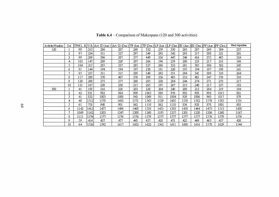
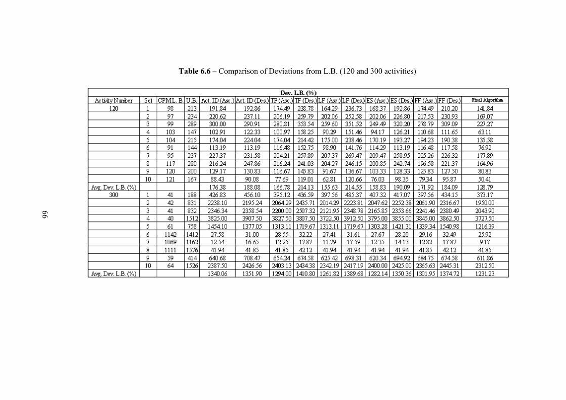
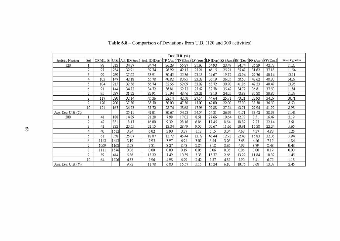
Experiment results show that the suggested algorithm outperforms the well

known commercial software packages; Primavera Project Planner (P6 version

7.0) and Microsoft Project 2010 for the RCPSP. In addition, the algorithm is

tested with problems obtained from literature as well as the benchmark

PSPLIB (Project Scheduling Problem Library) problems. The proposed

algorithm obtained satisfactory results especially for the problems with 120 and

300 activities. Limitations of the proposed genetic algorithm are addressed and

possible further studies are advised.

Keywords: Project Management and Scheduling, Resource-Constraints,

Genetic Algorithms.

vi

ÖZ

KISITLI KAYNAKLI İŞ PROGRAMLAMASI PROBLEMİNİN GENETİK

ALGORİTMALAR İLE ÇÖZÜLMESİ

Özleyen, Erdem

Yüksek Lisans, İnşaat Mühendisliği Bölümü

Tez Yöneticisi: Doç. Dr. Rıfat Sönmez

Ekim 2011, 91 Sayfa

Kısıtlı kaynaklı iş programlaması problemi faaliyetlerin öncelik sırasını ve

kaynak kısıtlarını dikkate alarak mümkün olan minimum proje süresini

bulmayı amaçlar. Bu problem polinomsal zamanda çözülebilen bir problem

olduğu için kesin sonucu bulmaya yönelik algoritmalar küçük boyutlu

projelerin çözümü ile sınırlıdır. Bu tezde sunulan genetik algoritma kesine

yakın sonuçları küçük projelerin yanında kesin çözüm algoritmalarının zayıf

olduğu büyük projeler için de bulmayı amaçlamaktadır. Geleneksel genetik

algoritmalara karşın, önerilen algoritma ileriye doğru planlama ile üretilen ve

geriye doğru planlama ile üretilen iki farklı popülasyon içerir. Genetik

algoritma sürecinde ileriye (geriye) doğru planlama ile yapılan iş takvimleri

geriye (ileriye) doğru planlama ile yapılan iş takvimlerine dönüştürülür.

Böylece, her iki tür takvimin karakteristikleri kullanılmış olur. Ayrıca, sunulan

algoritma eşleştirilecek bireyleri kaynakları kullandığı döneme göre seçerek

yeni bir çaprazlama operatörü sunmaktadır. Kullanılan mutasyon operatörü ise

sadece iyileşen iş takvimlerini popülasyona dahil edecek şekilde yapılmıştır.

Test sonuçları, önerilen algoritmanın sektörde iyi bilinen ve kısıtlı kaynaklarla

iş programlaması yapabilen Primavera Proje Planlayıcısı (P6 versiyon 7.0) ve

vii

Microsoft Project 2010 paket programlarına göre daha iyi olduğunu

göstermektedir. Ayrıca, sunulan algoritma literatürdeki benzer çalışmalarda yer

alan problemlerin çözümünde ve proje programlama problem

kütüphanesindeki örnek problemlerin çözümünde başarılı sonuçlar elde

etmiştir. Sunulan algoritma özellikle problem kütüphanesindeki 120 ve 300

aktiviteli projeler için tatmin edici sonuçlar vermiştir. Geliştirilen algoritmanın

sınırları ve ileride yapılabilecek iyileştirmeler ile ilgili öneriler yapılmıştır.

Anahtar Kelimeler: Proje Yönetimi ve Planlaması, Kaynak Kısıtlamaları,

Genetik Algoritmalar.

viii

This thesis is dedicated to my beloved family…

ix

ACKNOWLEDGEMENTS

I feel it is a unique privilege, combined with immense happiness, to

acknowledge the contributions and support of all the wonderful people who

have been responsible for the completion of my master degree.

I would like to express my deepest gratitude to my thesis advisor, Assoc. Prof.

Dr. Rıfat Sönmez who continually encouraged and guided me during the

course of my thesis work. I am grateful not only for his patient supports

throughout this study, but also for his modesty in sharing his valuable experiences

with me. I know that the insight he provided will guide me all through my life.

I want to gratefully thank to my teachers, Prof. Dr. Talat Birgönül and Kerem

Tanboğa for their unlimited support, encouragement, and love. It was their endless

trust and motivations that made me strong enough to pass all these steps.

I also want to express my thanks to my dear friends Emre Caner Akçay, Nuray

Gökdemir, Gülşah Fidan, and Mahdi Abbasi Iranagh who encouraged me with

their invaluable friendships throughout the accomplishment process of this thesis.

I would also like to express my great thanks to my dear brother Alp Özleyen for

his continuous love and support.

Finally, but most importantly, I would like to thank my mother Rana Özleyen

and my father Mehmet Vefa Özleyen. They bore with me, raised me, taught me

and made me who I am. No one deserves more appreciation and sincere thanks

than they do. I am truly blessed to have the privilege of being their son.

x

TABLE OF CONTENTS

ABSTRACT............................................................................................. iv

ÖZ ............................................................................................................ vi

ACKNOWLEDGEMENTS..................................................................... ix

LIST OF TABLES.................................................................................. xii

LIST OF FIGURES ............................................................................... xiv

LIST OF ABBREVIATIONS................................................................ xvi

1. INTRODUCTION............................................................................ 1

2. LITERATURE REVIEW................................................................. 5

2.1 Heuristic, Exact and Meta-heuristic Methods .................................. 5

2.2 Heuristic and Meta-heuristic Methods for RCPSP........................... 6

2.2.1 Heuristic Methods for RCPSP........................................... 6

2.2.2 Meta-heuristic Methods for RCPSP .................................. 8

3. GENETIC ALGORITHMS............................................................ 19

3.1 Research Method............................................................................ 19

3.2 Basics of the Genetic Algorithm .................................................... 19

3.2.1 Initial Population ............................................................. 21

3.2.2 Fitness Calculation .......................................................... 21

3.2.3 Selection .......................................................................... 21

3.2.4 Crossover......................................................................... 22

3.2.5 Mutation .......................................................................... 24

3.2.6 Replacement .................................................................... 25

3.2.7 Termination ..................................................................... 25

xi

4. RESOURCE CONSTRAINED PROJECT SCHEDULING

PROBLEM ..................................................................................... 27

4.1 Problem Formulation...................................................................... 27

4.2 Heuristic Procedures....................................................................... 29

4.2.1 Scheduling Schemes........................................................ 30

4.2.1.1 The Serial Scheduling Schemes ....................... 31

4.2.1.2 Priority Rule ..................................................... 33

4.2.1.3 Representation Scheme .................................... 34

5. CHARACTERISTICS OF THE DEVELOPED GENETIC

ALGORITHM ................................................................................ 35

5.1 Reading the Data from the Problem File........................................ 37

5.2 Building the Initial Population ....................................................... 38

5.3 Parent Selection and Crossover Procedure..................................... 50

5.4 Mutation Procedure ........................................................................ 57

6. COMPUTATIONAL RESULTS ................................................... 59

6.1 Computational Results ................................................................... 59

6.2 Comparison with Primavera Results .............................................. 61

6.2.1 T-Test for Controlling the Statistical Significance.......... 69

6.3 Comparison with Published Articles .............................................. 71

7. SUMMARY AND CONCLUSION............................................... 81

REFERENCES ....................................................................................... 85

xii

LIST OF TABLES

Table 2.1 Heuristic and Meta-heuristic Methods for RCPSP ...................16-18

Table 4.1 Project Information for Problem Formulation ..........................28

Table 4.2 Project Information for Scheduling Scheme .............................30

Table 5.1 Conversion of Successor to Predecessor of the Problem ..........39

Table 5.2 Generation Procedure of Left-Justified Schedules....................40-42

Table 5.3 Generation Procedure of Right-Justified Schedules..................43-45

Table 5.4 Completed Left-Justified Example Schedule ............................46

Table 5.5 Generation Procedure of Right-Justified Schedules..................46

Table 5.6 Example Project Information for Crossover Operator ..............53

Table 5.7 Random Key Values of the Crossover Operator .......................55

Table 6.1 Computational Results Other Alternatives................................60

Table 6.2 Computational Results of PSPLIB Problems............................60

Table 6.3 Comparison of Makespans (30 and 60 activities) .....................63

Table 6.4 Comparison of Makespans (120 and 300 activities) .................64

Table 6.5 Comparison of Deviations from L.B. (30 and 60 activities) .....65

Table 6.6 Comparison of Deviations from L.B. (120 and 300 activities) .66

Table 6.7 Comparison of Deviations from U.B. (30 and 60 activities) ....67

Table 6.8 Comparison of Deviations from U.B. (120 and 300 activities) 68

Table 6.9 T Test.........................................................................................69-70

Table 6.10 T Test Results..........................................................................70

Table 6.11 The Network Data of 1st Case .................................................72

Table 6.12 The Best Found Schedule by Final Algorithm for 1st Case.....73

Table 6.13 The Network Data of 2nd Case ................................................74

Table 6.14 The Best Found Schedule by Final Algorithm for 2nd Case ....75

Table 6.15 The Resource Constraints of the Projects ...............................77

Table 6.16 The Project Makespans from Different Approaches ...............78

Table 6.17 The Best Found Schedule by Final Algorithm for 1st Project .78

xiii

Table 6.18 The Best Found Schedule by Final Algorithm for 2nd Project 79

Table 6.19 The Best Found Schedule by Final Algorithm for 3rd Project.79

xiv

LIST OF FIGURES

Figure 3.1 Flowchart of a Basic GA..........................................................20

Figure 3.2 Crossover Operator ..................................................................22

Figure 3.3 Non-efficient Crossover Operator............................................23

Figure 3.4 Mutation Operator....................................................................24

Figure 3.5 Outline of the Basic GA...........................................................26

Figure 4.1 Activity-on-Node Relationship Graph for Problem

Formulation ...............................................................................................28

Figure 4.2 Schedule of Minimum Project Duration for Problem

Formulation ...............................................................................................29

Figure 4.3 Schedule of Minimum Project Duration for Scheduling

Scheme ......................................................................................................31

Figure 4.4 Solution Obtained by Forward Serial Scheduling Scheme......32

Figure 4.5 Solution Obtained by Backward Serial Scheduling Scheme ...33

Figure 5.1 Pseudo-Code of Proposed Genetic Algorithm.........................36

Figure 5.2 Example Problem File..............................................................37

Figure 5.3 Assigning the Left-Justified Schedule Start Time ...................47

Figure 5.4 Completed Left-Justified Schedule of Example Problem........48-49

Figure 5.5 Sorting Mechanism of the Algorithm ......................................50

Figure 5.6 Parent Selection Pool ...............................................................51

Figure 5.7 Precedence Chart of Example Project for Crossover

Operator.....................................................................................................53

Figure 5.8 The Schedule of Father for Crossover ....................................54

Figure 5.9 The Schedule of Mother for Crossover....................................54

Figure 5.10 RUR Profile of Father ............................................................55

Figure 5.11 The Schedule of Child ...........................................................56

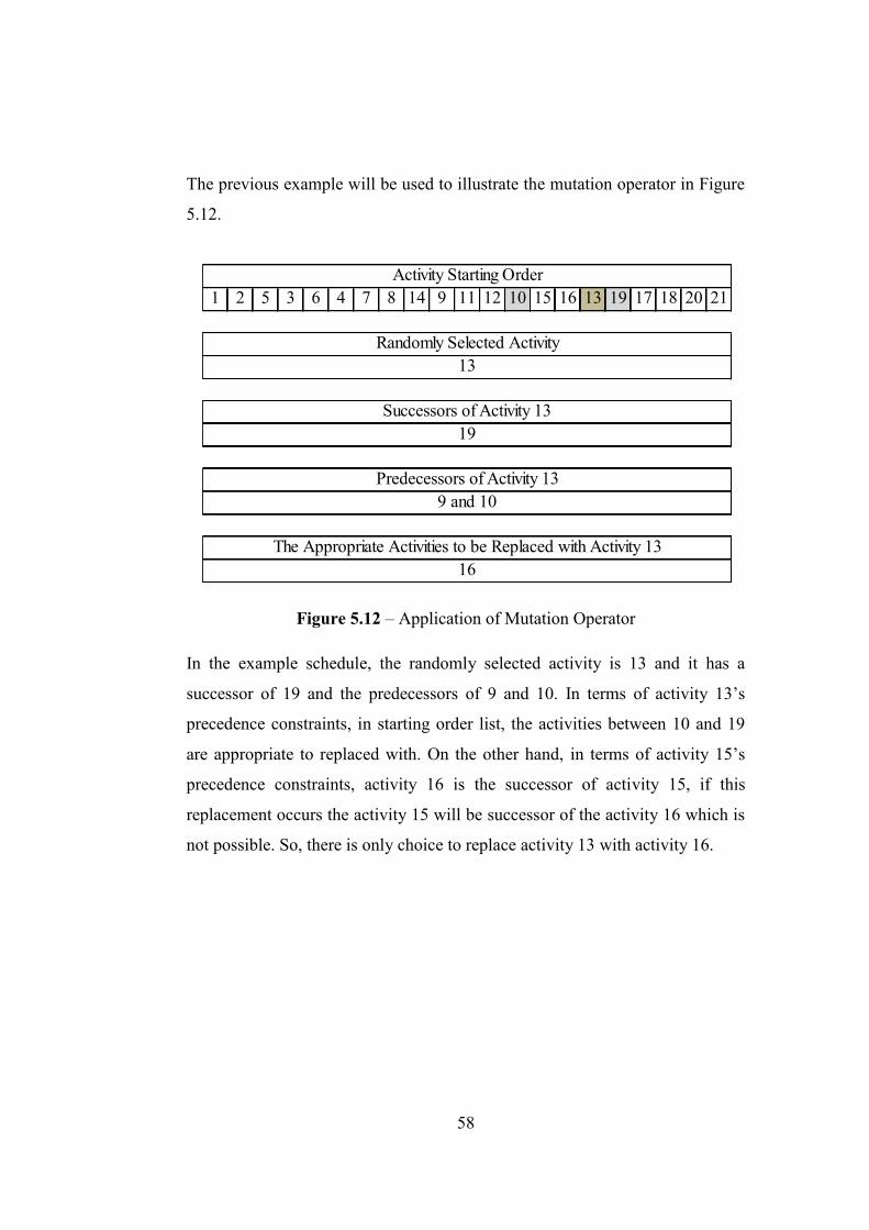
Figure 5.12 Application of Mutation Operator .........................................58

Figure 6.1 The Initial Gantt Chart for 1st Case ..........................................72

xv

Figure 6.2 The Best Found Schedule by Published Article for 1st Case....73

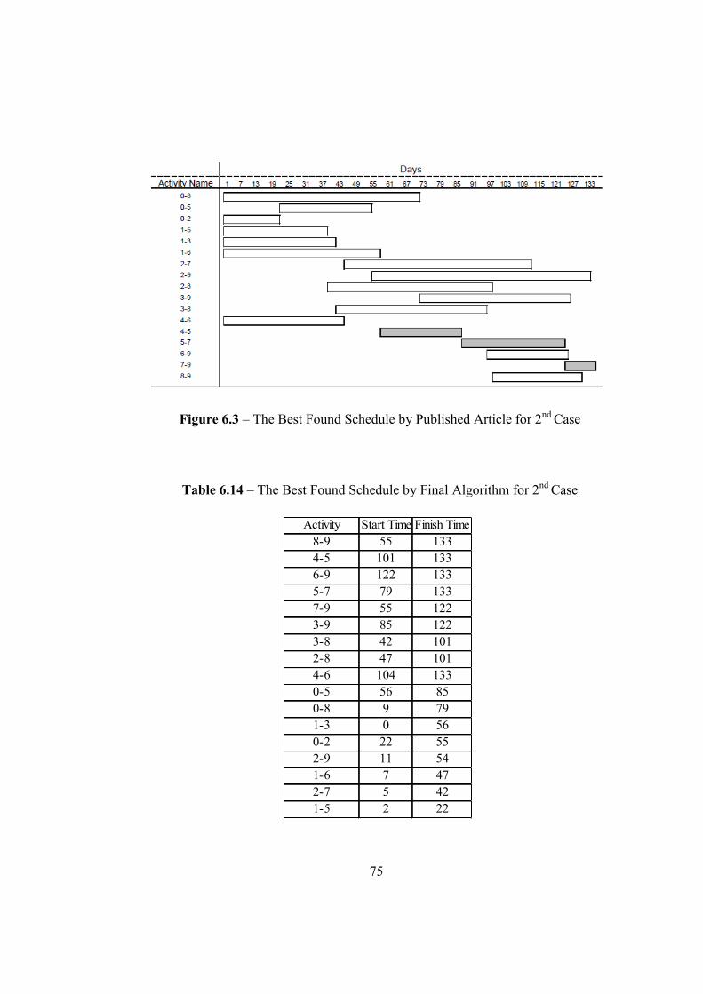
Figure 6.3 The Best Found Schedule by Published Article for 2nd Case...75

Figure 6.4 Project Network for the 1st Project...........................................76

Figure 6.5 Project Network for the 2nd Project..........................................76

Figure 6.6 Project Network for the 3rd Project ..........................................77

xvi

LIST OF ABBREVIATIONS

PSPLIB Project Scheduling Problem Library

CPM Critical Path Method

ES Early Start

EF Early Finish

LS Late Start

LF Late Finish

RCPSP Resource-Constrained Project Scheduling Problem

RLP Resource Leveling Problem

RCP Resource-Constrained Projects

NP-hard Non-Deterministic Polynomial-Time Hard

J30 Problem Set with 30 Activities




SGS Schedule Generation Scheme

GA Genetic Algorithm

BPGA Bi-Population Genetic Algorithm

rc-mPSP Resource-Constrained Multi Project Scheduling Problem

CPU Central Processing Unit

ACO Ant Colony Optimization

PSO Particle Swarm Optimization

ALA Adaptive-Learning Approach

AugNN Augmented Neural Network

HNA Hybrid Neural Approach

DBGA Decomposition-Based Genetic Algorithm

HGA Hybrid Genetic Algorithm

F&F Filter-and-Fan

xvii

SA Simulated Annealing

AIA Artificial Immune Algorithm

SS Scatter Search

OOP Object-Oriented Programming

GRASP Greedy Randomized Adaptive Search Procedure

TS Tabu Search

NN Nearest Neighbor

RUR Resource Utilization Ratio

TRU Total Resource Utilization

RK Random Key

UB Upper Bound

LB Lower Bound

1

CHAPTER 1

INTRODUCTION

Project completion within a time limit is substantial for successful project

performance, regardless of the size and complexity of the project. Each day of

delay in the completion time causes a loss in revenue that can hardly be

regained later. Project scheduling involves the construction of a plan which

specifies for each activity the precedence, resource feasible start and finish

dates, the amounts of the various resource types that will be needed during

each time period and as a result the budget. Good scheduling can obviate

problems and insures the completion of a project on time. In contrast, poor

scheduling can result in significant idle labor and equipment. Obviously,

project scheduling is an important and elaborate task in the management and

delivery of construction projects.

Construction scheduling involves the definition of activities, the estimation of

durations for individual activities, establishment of the relations between

activities, and the required resources for undertaking activities. Thus, project

management must decide which resources are going to be used for the

execution of a project, must decide on the capacity of the various resource

types and must estimate the resource requirements for the project activities.

Apparently, if these resources are adequate, then the project could be executed

to attain expected project duration. On the other hand, if these resources are

limited, then more likely there will be a delay in the project completion time.

As a matter of fact, a sufficient schedule, which integrates resources properly,

provides competitive benefit to the company during project period.

2

Critical Path Method (CPM) is the one of the most widely used scheduling

technique. In CPM, early start and finish dates, and late start and finish dates

are calculated for all tasks without considering any resource limitations by

carrying out forward and backward scheduling procedures. On any schedule

network, the schedule flexibility is determined by the difference between late

and early dates, and is called “total float”. Critical paths have a zero total float

and activities on a critical path are termed “critical activities” which means any

delay in these activities cause a delay in whole project duration. On the other

hand, the activities that have positive float can be regarded as flexible and these

activities can be postponed according to their float values.

Theoretically, in CPM, if precedence relations and activity durations are

defined correctly, resource allocation may not be performed. In fact, in

construction industry, resource issues are generally ignored. Therefore,

Resource Leveling Problem (RLP) and Resource Constrained Project

Scheduling Problem (RCPSP) occur where unleveled use of resources exists

throughout the project duration and the available amounts of resources does not

meet with resource requirements respectively. Thus, to prevent these, resource

utilization charts should be evaluated in detail.

In many project scheduling, resource usage throughout the project might be

much more critical than the peak usage of the schedule. The aim of Resource

Leveling Problem (RLP) is to prevent fluctuations on the resource usage

graphs. In other words, solution of RLP aims completing the project within

time with a resource utilization chart which is as balanced as possible over

project makespan.

Scheduling problems involve many types of constraints. Resource constrained

project scheduling problem (RCPSP) emerges when there are limits on the

availability of resources. Obtaining an adequate solution for the RCPSP is

3

crucial for scheduling and planning of construction projects. Ineffective

allocation of resources because of inappropriate scheduling of resource

constrained projects (RCP) will increase the project duration and cost

considerably. The solution of RCPSP addresses a schedule of minimum

duration by assigning a start date to each task such a way that the precedence

relations and resource constraints are satisfied.

In general concept of RCPSP, a set of activities, resources, constraints are

given and the objective is to obtain minimum project makespan by satisfying

precedence and resource constraints in the project. In order to understand the

RCPSP clearly, general assumptions of the problem outlined as follows;

If an activity does not have a precedence and resource constraints, that

activity must be started without any delay.

Resources are constrained and if there is no adequate resource, the

activity must start following appropriate day when there is a necessary

resource exist.

If an activity has started, it cannot be interrupted.

Resource requirements, resource availabilities, activity durations, and

precedence constraints are constant throughout the project horizon.

The RCPSP is one of the most difficult optimization problems. Indeed, the

RCPSP is a polynomial-time hard (NP-hard) problem, meaning the problem

cannot be solved by exact algorithms for finding exact solution in reasonable

time. Some exact methods exist only for the small projects and also they take

more than polynomial time when the project grows or extra resource

constraints are added. Therefore, most research studies have been devoted to

improve heuristic and meta-heuristic procedures to obtain near-optimal

solutions within a polynomial time. Further information on both exact and

heuristic methods is going to be introduced in the next chapter.

4

The objective of this study is to present a genetic algorithm which solves

RCPSP to produce near-optimal solutions within an acceptable computation

time. C++ programming language has been used and proved to conveniently

operate on different problem sets. It is an meta-heuristic method which differs

from earlier studies both in terms of the crossover operator and parent selection

mechanism. Different problem sets which include 30, 60, 120, and 300

activities are used and test results are presented for performance analysis

purposes. The study is planned as in the following: Chapter 2 focuses on

heuristic, exact, and meta-heuristic methods and also includes related literature

about RCPSP. In Chapter 3, information on the genetic algorithm is presented.

Chapter 4 includes problem formulation, information about scheduling

schemes, priority rule, and representation scheme. Chapter 5 describes the

methodology of generated genetic algorithm. Chapter 6 introduces some other

developed alternatives of the proposed algorithm and the computational results

of the algorithm. Chapter 7 presents the conclusion part of the thesis.

5

CHAPTER 2

LITERATURE REVIEW

The Resource Constrained Project Scheduling Problem (RCPSP) has been

widely studied in the field of scheduling, resulting in a comprehensive variety

of optimization techniques. Many solution models have been suggested and

carried out and 3 methods have been emphasized for the problem: heuristic

methods, exact methods, and meta-heuristic methods.

2.1 Heuristic, Exact and Meta-heuristic Methods

The word heuristic has arisen after the Greek word “heuriskein” meaning to

discover. Heuristic methods have been also known as seeking method in

literature. This technique searches for satisfactory (i.e. near-optimal) solutions

at an acceptable solution time without being able to ensure that the solution is

feasible or optimal. Most known heuristics are construction heuristics and

improvement heuristics. In constructive heuristics, a solution is constructed

according to some construction rules and it continues step by step and it does

not try to improve the solution. On the other hand, in improvement heuristics, a

solution is constructed and initial solution is improved as soon as possible.

Exact methods are used to find the optimal solution to the RCPSP. Due to

exploring the search space deeply exact methods are not efficient especially for

large size problems. Thus, they generally cooperate with heuristics and they are

used as a part of heuristics. Some of the popular exact methods can be listed as;

linear programming based approaches, branch-and-bound procedures, dynamic

programming etc.

6

Meta-heuristic methods are similar to heuristics in terms of finding not optimal

solution but meta-heuristics are more likely not to be stuck in a local optimal

solution because repetitious moves are prevented in algorithm. Some of the

popular meta-heuristic methods can be listed as; simulated annealing, genetic

algorithms, particle swarm optimization, tabu search etc.

As indicated in previous chapter, RCPSP belongs to the class of the NP-hard

problems (Blazewicz et al., 1983) which expresses that solution time for

achieving the optimal solution by using exact methods can be considerable

long. Integer programming methods and branch-and-bound procedures are the

main algorithms that are used for the RCPSPs’ exact solution. In addition,

exact methods can only solve small size problem instances with up to

approximately 60 activities in an acceptable manner. Even though, heuristic

methods and meta-heuristic methods do not guarantee optimality and find near-

optimal solution, they are accepted as practical procedures to solve RCPSP

because of their handling capacity of large size problems, adjustability, and

easy implementation. Thus, because of their capability to solve large size

projects they can reflect the reality more than exact procedures.

2.2 Heuristic and Meta-heuristic Methods for RCPSP

2.2.1 Heuristic Methods for RCPSP

An experimental survey of heuristics for RCPSP has been published by

Kolisch and Hartmann (2006). In this study, a large number of studies that

have been proposed until 2005 have been outlined and categorized. They also

have evaluated and compared heuristics. Also, they have addressed

characteristics of good heuristics. In comparison, average deviations (%) from

optimal solutions and for unknown optimal solutions, average deviations (%)

from the well-known critical path lower bounds have been considered.

7

According to test results, for the J30, J60 and J120 problem sets, the top five

state-of-the-art algorithms are (Kochetov and Stolyar, 2003), (Debels et al.,

2004), (Valls et al., 2003), (Valls et al., 2005), and (Alcaraz et al., 2004).

According to these studies, features of the state-of-the-art algorithms can be

listed as follows;

Essential part in future heuristics for the RCPSP will be forward-

backward improvement.

Both scheduling directions (forward scheduling and backward

scheduling) have been considered instead of only one direction.

Both serial and parallel schedule generation scheme (SGS) have been

regarded instead of only one.

State-of-the-art algorithms have considered multiple local search

operators or even multiple meta-heuristic strategies.

Another heuristic algorithm based on filter-and-fan method has been

introduced by Ranjbar (2008). The local search has been used to investigate

solution space and to produce first solution. Filter-and-fan method is a local

search process that produces moves in a three search manner. It is a compound

of a local search and filter-and-fan (F&F) search. The method has analyzed the

local optimum and searched greater area to prevent getting stuck in a local

optimum.

Seda et al. (2009) has proposed a flexible heuristic algorithm for resource-

constrained project scheduling problem. They have suggested a heuristic that

differ from classical activity shifting when the resource availability has been

surpassed. This heuristic has decided the activities that should be started as

soon as possible and the activities that should be delayed. Further

investigations have been suggested as a fuzzy variant of the problem and

8

application of the algorithm on a resource-constrained multi project scheduling

problem (rc-mPSP).

Anagnostopoulos and Koulinas (2011) have been proposed a Greedy

Randomized Adaptive Search Procedure (GRASP) based hyper-heuristic for

RCPSP. This algorithm consists of two steps: a creation stage and a local

search step. In creation step, feasible solutions have been produced and in

continuation, neighborhood of solutions has been analyzed to find the best

solution (local minimum) in neighborhood. During construction of candidate

solutions, each element has been selected according to their benefits to the

solution. For further research, solution representation scheme could be changed

and local search technique could be simulated annealing or tabu search.

2.2.2 Meta-heuristic Methods for RCPSP

Kochetov and Stolyar (2003) have proposed an evolutionary algorithm built on

path re-linking strategy and tabu search with variable neighborhood. Path re-

linking method has been used for crossover operator. Firstly, multiple paths

between selected solutions from the population have been built. Secondly, they

have selected one of the paths and improved it by tabu search algorithm. Then,

the enhanced solution has been added to population and the worst solution has

been eliminated. At the end of the evolution, diversification methodology has

been performed.

A new meta-heuristic to solve RCPSP has been presented by Debels et al.

(2004). This method has proved that this algorithm was capable to solve

relatively large size problems. This study is a combination of a population-

based meta-heuristic, scatter search (SS), and a heuristic method based on

electromagnetism theory.

9

Valls et al. (2005) have been introduced a justification technique that can be

easily integrated to different algorithms without increasing the computation

time. Justification is a simple and easily incorporable technique that boosts the

algorithm and creates better schedules. Three dissimilar algorithms which are

well-known, simple, and complex introduced by Hartmann (1998) have been

tested. In all type of algorithms, double justification has enhanced the solutions

and decreased the CPU time by 30%. They have incorporated double

justification in 22 diverse heuristic algorithms and fifteen of the new

algorithms that use double justification have outperformed seven of the best

heuristic algorithms that do not use justification Valls et al. (2005). Thus, they

have strongly recommended adding double justification to the algorithms.

Debels and Vanhoucke (2005) have proposed a genetic algorithm (GA) which

has used two different populations. They have called that study bi-population

genetic algorithm (BPGA). In this algorithm, left-justified (forward) and right-

justified (backward) scheduling methods have been operated to take advantage

of both scheduling techniques. Left-justified schedules have been used to

create right-justified schedules and vice versa.

Another meta-heuristic method to solve RCPSP has been presented by Mendes

at al. (2005). This genetic algorithm has been based on random keys in terms of

chromosome representation and they have used a heuristic priority rule in

which genetic algorithm determines priorities of the algorithms. The study has

been tested on standard examples and compared with other approaches in the

literature and considerable good results have been obtained Mendes at al.

(2005).

Tseng and Chen (2006) have presented a hybrid meta-heuristic for the RCPSP

that integrated genetic algorithm (GA), ant colony optimization (ACO), and

local search strategy. They have named this algorithm, ANGEL. In this study,

10

firstly, solution space has been explored and task list has been generated to

create the initial population for GA. Next, ACO pheromone sets have been

updated with the GA solutions with the condition that GA obtains a better

solution. When, GA has been completed, ACO has been started to search by

using new set. By the same way, GA and ACO have searched the solution in

the solution space until termination of GA and ACO. From this paper, it has

been remarked that local search strategy is very efficient and ANGEL is very

effective.

Debels and Vanhoucke (2006) have suggested a decomposition approach

which has divided the problem sets into smaller problems to be figured out

with an exact or heuristic algorithm and have combined the solutions from sub-

problems to obtain the solution of the problem sets. After, advanced

neighborhood search have been proposed. During decomposition process,

meta-heuristic and exact procedures from literature have been used to extend

this study. Computational results have showed that conventional meta-

heuristics have not enough time to comprehensively explore the whole solution

space and the decomposition approach has led to better results. In addition to

this, sub-problems should be large enough to find better solutions for the main

problem sets, and small enough to prevent unreasonable computation times.

Particle swarm optimization (PSO) to solve RCPSP has been proposed by

Zhang et al. (2006). In this study, particles have represented the activities

priorities, so that optimal solution can be sought from an updated population

according to particle swarm optimization method used. The tests have showed

that the PSO-based method for RCPSP capable to seek for global optima. Also,

PSO is better than GA in terms of search mechanism. Detailed consideration

on PSO parameters, application of PSO, and interface of the program have

been addressed for further researches.

11

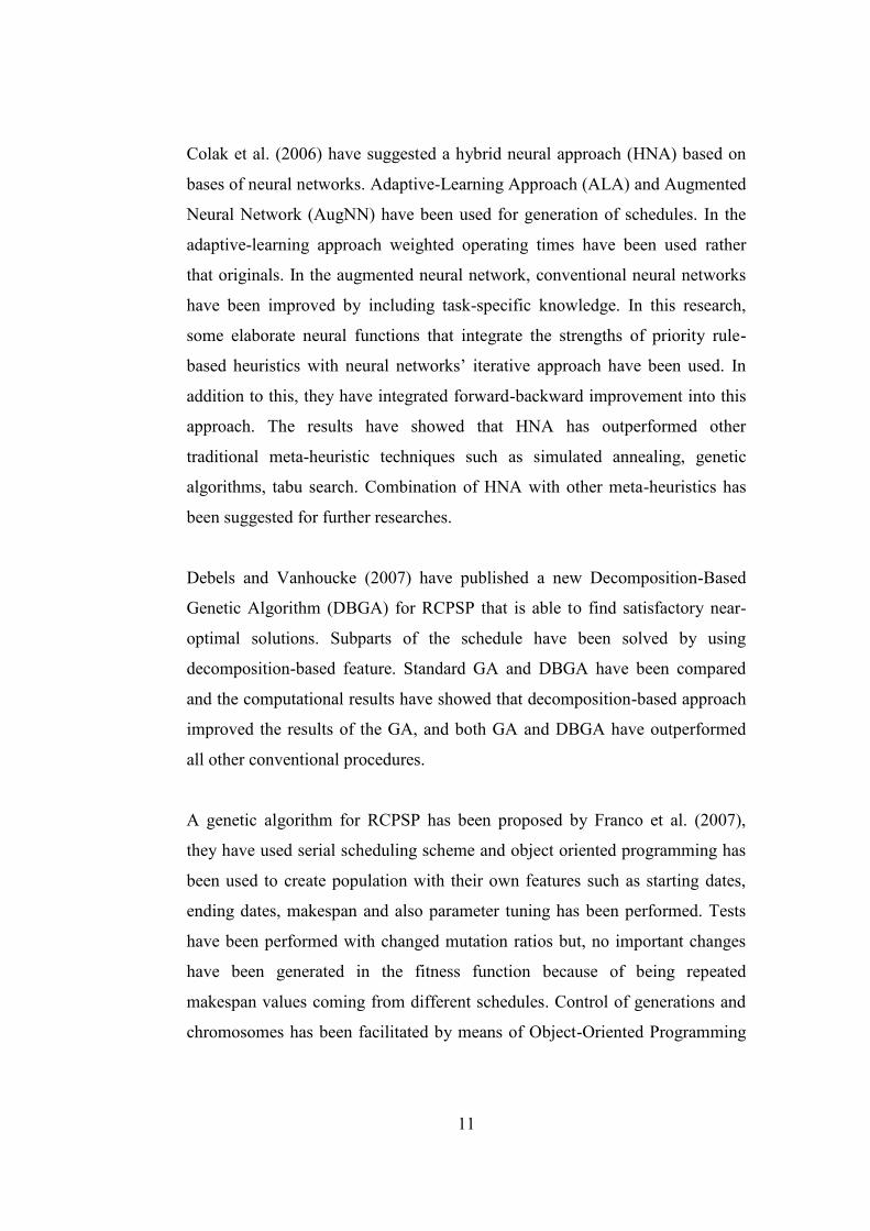
Colak et al. (2006) have suggested a hybrid neural approach (HNA) based on

bases of neural networks. Adaptive-Learning Approach (ALA) and Augmented

Neural Network (AugNN) have been used for generation of schedules. In the

adaptive-learning approach weighted operating times have been used rather

that originals. In the augmented neural network, conventional neural networks

have been improved by including task-specific knowledge. In this research,

some elaborate neural functions that integrate the strengths of priority rule-

based heuristics with neural networks’ iterative approach have been used. In

addition to this, they have integrated forward-backward improvement into this

approach. The results have showed that HNA has outperformed other

traditional meta-heuristic techniques such as simulated annealing, genetic

algorithms, tabu search. Combination of HNA with other meta-heuristics has

been suggested for further researches.

Debels and Vanhoucke (2007) have published a new Decomposition-Based

Genetic Algorithm (DBGA) for RCPSP that is able to find satisfactory near-

optimal solutions. Subparts of the schedule have been solved by using

decomposition-based feature. Standard GA and DBGA have been compared

and the computational results have showed that decomposition-based approach

improved the results of the GA, and both GA and DBGA have outperformed

all other conventional procedures.

A genetic algorithm for RCPSP has been proposed by Franco et al. (2007),

they have used serial scheduling scheme and object oriented programming has

been used to create population with their own features such as starting dates,

ending dates, makespan and also parameter tuning has been performed. Tests

have been performed with changed mutation ratios but, no important changes

have been generated in the fitness function because of being repeated

makespan values coming from different schedules. Control of generations and

chromosomes has been facilitated by means of Object-Oriented Programming

12

(OOP). They have also observed that two-point crossover brought better

schedules even at solution times. As a further research, usage of this algorithm

has been proposed for multi-mode project scheduling problems and calibration

of different parameters such as size of population, number of generations,

crossover operator etc. have been suggested.

Another Hybrid Genetic Algorithm (HGA) has been proposed for the RCPSP

by Valls et al. (2008). Various changes have been made in the conventional

GA algorithm: resource-constrained project scheduling specific crossover

method; an enhancement operator for generated schedules; a new parent

selection mechanism; and a two-step approach which have allowed starting the

evolution from best schedule of the neighbor’s population. To be more

detailed, they have used the crossover operator that combines favorable parts of

the solutions instead of general crossover period that randomly selects parts of

the solutions. Double justification operator Valls et al. (2005) has been used for

schedule improvement. In addition, they have allowed the first individual in the

couple to be the best individual in the population and the other individual has

been selected randomly from the rest of the population. Therefore, they have

guaranteed that fittest individuals have been used once as parents.

Kim and Ellis (2008) have presented permutation-based elitist genetic

algorithm especially for large-sized projects. Elitist selection mechanism has

been used to keep the fittest individual in the population and SGS has been

applied to create feasible individual to the problem. In addition to these, the

one-point crossover, standard mutation operator, and a random number

generator have been used. In this study, first generation has been generated by

a random number generator that has incorporated with precedence and resource

constraints. In SGS, all precedence and resource feasible activities have been

grouped and activities have been selected one by one to generate a feasible

individual. During elitist selection, the best individual has been preserved for

13

the next generation to assure that fittest solution has been kept. For further

research, they have suggested to use two-point crossover or different cross-

over operators and a hybrid-heuristic algorithm to improve the solutions, and

the tournament selection to overcome the drawback of the roulette wheel

selection.

A Genetic algorithm with simulated annealing for RCPSP has been published

by Xiaoguang et al. (2009). The algorithm has been integrated with simulated

annealing (SA) to better local searching and to encourage the progress. In each

generation, the algorithm has produced a new substitute population and for

improvement SA has been applied to every individual. For convergence’s sake,

the cooling process has been occurred at the end of each loop and advancing

speed of the algorithm has been suggested as a further research by authors.

Mobini et al. (2009) have proposed another state-of-the-art algorithm that

named as enhanced scatter search algorithm for the RCPSP. The new algorithm

has been established on a new path re-linking strategy, permutation based and

conventional two-point crossover operators Mobini et al. (2009). Scatter search

is a population-based method that has produced new individuals by associating

maintained solution. First, the initial generation has been produced by

diversification generation method. Second, the improvement method has been

performed to modify solution to improved solution. Third, the reference set

update method has collected the solutions according to their fitness and

diversity. Fourth, the subset generation method has been used to group the

solutions into subsets. Lastly, the combination method has been used that

consist of the path re-linking, permutation-based operator and traditional two-

point crossover operator Mobini et al. (2009). They have concluded that

according to CPU time and quality of the solutions their algorithm can be

considered as the second best algorithm after Valls et al. (2004).

14

Bettemir (2009) has proposed another meta-heuristic algorithm that finds

optimum or near optimum solutions for the time cost trade-off, resource

leveling, and resource-constrained project scheduling problems. In the solution

of the RCPSP, the traditional genetic algorithm has been used and only the

problem sets up to 120 activities have been solved. In addition, the proposed

algorithm’s performance was not compared with commercial software

packages such as; Primavera Project Planner or Microsoft Project.

Mobini et al. (2010) have proposed an artificial immune algorithm (AIA) for

the RCPSP. Objective function and generated solution have been converted to

their equivalents in AIA which are antigen and antibody respectively. In this

algorithm generation of schedules which have lower makespan have a more

chance to be generated in the next population. In addition, serial-SGS has been

used to decode the representation and improved method has been applied to the

initial population instead of traditional randomly generated initial generation.

In this study, right-justified (backward) schedules and left-justified (forward)

schedules have been generated to improve initial generation. In addition, to

assist the convergence of AIA, point-mutation and multi-point mutation have

been used on every candidate solution.

Chen et al. (2010) have suggested an efficient hybrid algorithm that combines

ant colony methodology, scatter search, and a local search progress. First, the

algorithm has explored all possible solutions and produced activity lists to

generate first population to scatter search. Second, scatter search has improved

the solutions. Thereafter, ant colony optimization has used these improved

solutions. In addition, local search algorithm has improved the makespan of

schedules and ant colony optimization has incorporated scatter search strategy

in searching solution space.

15

A new efficient genetic algorithm has been proposed by Hong et al. (2010). In

this study, selection of schedule generation scheme (SGS) has been added as a

feature to decoding progress and forward-backward improvement has been

applied to all population. In addition, elitist selection and an effective parent

selection mechanism have been used to improve the algorithm.

Torres et al. (2010) have been proposed a genetic algorithm for the RCPSP. In

this paper, object-oriented model has been used to representation of schedules.

Thereby, they have taken advantages of programming languages. The classes

have been used in object-oriented programming (OOP) for representation of

schedules. In addition, the OOP has made the progress more controllable and

flexible.

Christodoulou (2010) has proposed a methodology to RCPSP by use of ant

colony optimization artificial agents. The utility value approach has been used

to decide which activity is going to get resources first. There are features that

have composed the utility value such as the total float of the activity, the

criticality index which has been calculated from Monte Carlo simulations, a

heuristic value which has been depended on importance of the activity, and a

cost value which is activity’s cost over the project’s total cost (Christodoulou,

2010). Convergence of this study as compared with other traditional heuristics

has been occurred faster and also as a further research, performance of the

algorithm on bigger problem sets such as J120 or J300 has been suggested.

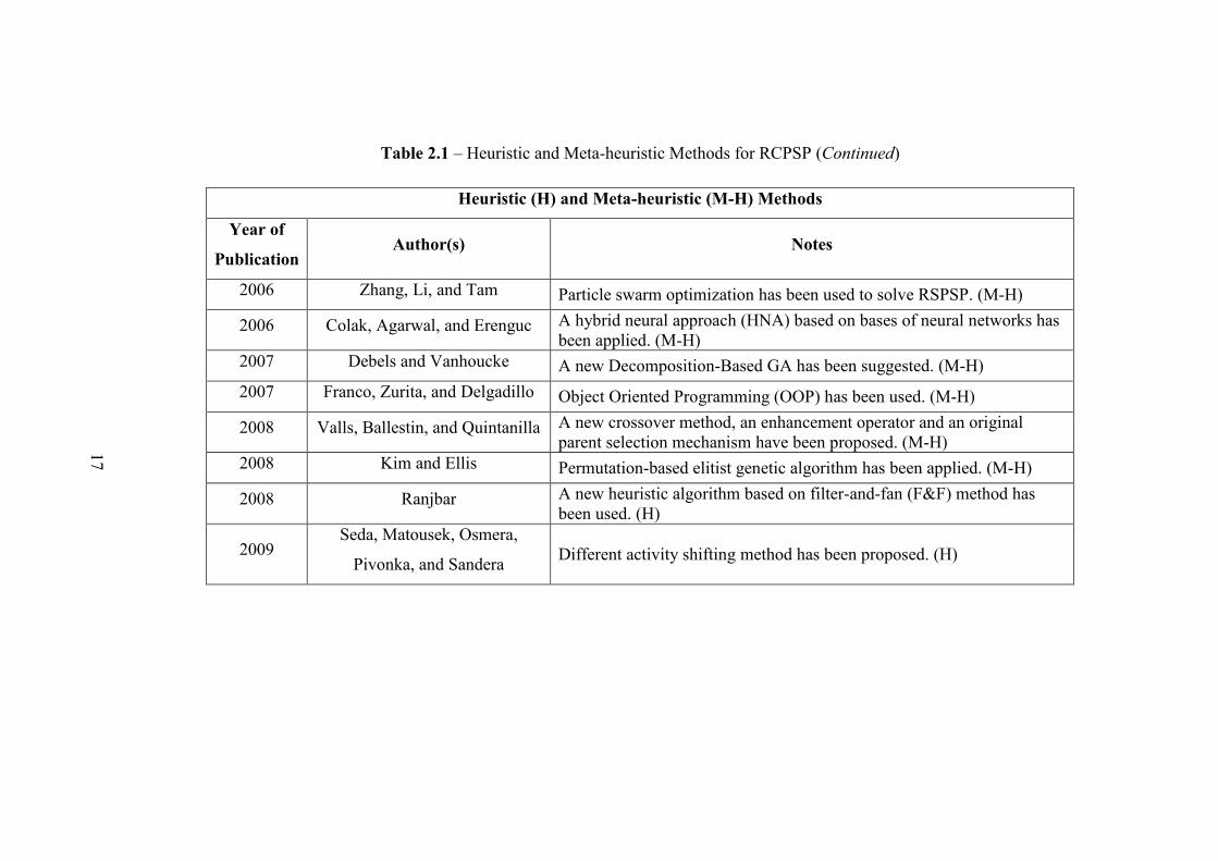
A brief summary of heuristic based methods for the solution of resource

constrained scheduling problem in this section can be seen in Table 2.1.

16

Table 2.1 – Heuristic and Meta-heuristic Methods for RCPSP

Heuristic (H) and Meta-heuristic (M-H) Methods

Year of

PublicationAuthor(s) Notes

2003 Kochetov and Stolyar Path re-linking strategy, tabu search, and diversification methodology hasbeen used. (M-H)

2004Debels, Reyck, Leus, and

VanhouckeBased on population-based meta-heuristic, scatter search (SS), and anelectromagnetism theory. (M-H)

2005 Valls, Ballestin, and Quintanilla Double justification technique has been introduced. (M-H)2005 Debels and Vanhoucke Left-justified and Right-justified schedules have been used in GA. (M-H)

2005 Mendes, Gonçalves, and Resende A different chromosome representation and priority rules have been used.(M-H)

2006 Tseng and Chen Ant colony optimization (ACO), and local search strategy has been applied.(M-H)

2006 Debels and Vanhoucke A decomposition approach where the solutions have been combined fromsub-problems to obtain the solution of the problem sets. (M-H)

2006 Kolisch and Hartmann Heuristics for resource-constrained project scheduling have beeninvestigated. (H)

17

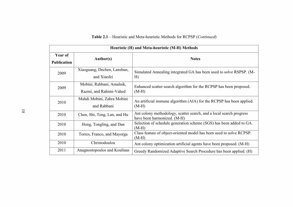
Table 2.1 – Heuristic and Meta-heuristic Methods for RCPSP (Continued)


Year of


2006 Zhang, Li, and Tam Particle swarm optimization has been used to solve RSPSP. (M-H)

2006 Colak, Agarwal, and Erenguc A hybrid neural approach (HNA) based on bases of neural networks hasbeen applied. (M-H)

2007 Debels and Vanhoucke A new Decomposition-Based GA has been suggested. (M-H)2007 Franco, Zurita, and Delgadillo Object Oriented Programming (OOP) has been used. (M-H)

2008 Valls, Ballestin, and Quintanilla A new crossover method, an enhancement operator and an originalparent selection mechanism have been proposed. (M-H)

2008 Kim and Ellis Permutation-based elitist genetic algorithm has been applied. (M-H)

2008 Ranjbar A new heuristic algorithm based on filter-and-fan (F&F) method hasbeen used. (H)

2009Seda, Matousek, Osmera,

Pivonka, and Sandera Different activity shifting method has been proposed. (H)

18

Table 2.1 – Heuristic and Meta-heuristic Methods for RCPSP (Continued)


Year of


2009Xiaoguang, Dechen, Lanshun,

and XiaofeiSimulated Annealing integrated GA has been used to solve RSPSP. (M-H)

2009Mobini, Rabbani, Amalnik,

Razmi, and Rahimi-VahedEnhanced scatter search algorithm for the RCPSP has been proposed.(M-H)

2010Mahdi Mobini, Zahra Mobini

and RabbaniAn artificial immune algorithm (AIA) for the RCPSP has been applied.(M-H)

2010 Chen, Shi, Teng, Lan, and Hu Ant colony methodology, scatter search, and a local search progresshave been harmonized. (M-H)

2010 Hong, Tongling, and Dan Selection of schedule generation scheme (SGS) has been added to GA.(M-H)

2010 Torres, Franco, and Mayorga Class feature of object-oriented model has been used to solve RCPSP.(M-H)

2010 Christodoulou Ant colony optimization artificial agents have been proposed. (M-H)2011 Anagnostopoulos and Koulinas Greedy Randomized Adaptive Search Procedure has been applied. (H)

19

CHAPTER 3

GENETIC ALGORITHMS

The first development in the field of Genetic Algorithms appeared in 1960s.

Impact of genetic algorithms has outshone other techniques, such as Tabu

Search (TS) or Simulated Annealing (SA). Fitness measurement of every

individual and selection of potential solutions to reproduce are the main

advantages of GA. Moreover, there is a recombination of different individuals

that allow genetic variation. Especially, for the NP-hard problems which are

very complex problems as mentioned before concept of evolution diversity is

an archetype.

3.1 Research Method

In this thesis, in addition to the traditional GA, a unique crossover operator and

parent selection mechanism are going to be presented. The PSPLIB problem

sets are going to be solved by Primavera and proposed algorithm. Moreover,

some problems from literature are going to be solved and the solutions are

going to be compared.

3.2 Basics of the Genetic Algorithm

The GA has arisen from the similarity between the representations of complex

structure and the genetic structure of a chromosome. In nature, for example,

offspring are sought which are persistent in terms of chromosome combination.

In a same way, during solution of complex structure, the individuals from

existing solutions are combined to get better individuals.

20

In common sense, the chromosomes are usually represented by simple string of

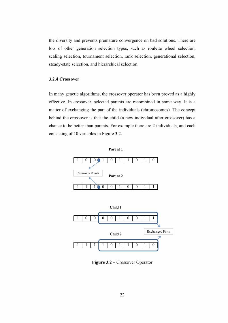
0s and 1s and several genetic operators have been recognized for controlling

these chromosomes, the most frequently used operators are crossover and

mutation. In other words, the changing feature is exchange of piece of the

chromosomes and a local adjustment of a variable in a chromosome.

For a NP-hard problem, such as resource-constrained project scheduling

problem, the genetic algorithm works by managing a population of potential

parents whose fitness (appropriateness) values have been computed. Each

chromosome encrypts a solution to the problem, and its fitness value depends

on the value of objective function for that solution. Traditional GA selects the

one parent depends on its fitness value (the bigger fitness value, the more

chance to being chosen) and the other parent is selected randomly from all

population. Then, crossover and mutation operator are performed and lastly,

the population are updated with new individuals, given in Figure 3.1.

Figure 3.1 – Flowchart of a Basic GA

Population

(chromosomes)

Fitness Evoulation

Selection

(Mating Pool)

Parents

Genetic Operators

(Crossover and Mutation)

21

3.2.1 Initial Population

Generating random individuals for initial population is the first step of genetic

algorithm. The main idea of population size is always of a trade-off between

effectiveness and efficiency. Small populations would cause the risk of not

exploring the solution space, while too large populations would cause impaired

efficient computation.

It is generally assumed that initial population should be generated randomly;

however, this approach doesn’t cover the solution space systematically when

compared with complex statistical methods. On the other hand, there is a

possibility of feeding the initial population with high-quality solutions,

obtained from other techniques. This approach would find the final solution in

less time. However, immature convergence risk would exist.

3.2.2 Fitness Calculation

Fitness evoulation is the second step after the generation of initial population.

Fitness values emphasize the quality of individuals (chromosomes) in the

population. The objective function is used to calculate fitness values and it is

simply to use objective function associated with each individual. However,

convergence to similar individuals, and premature convergence to a local

optimum because of being only a few good individuals in the population

should be considered.

3.2.3 Selection

The main idea behind the selection is that the selection should be related to

fitness value of the individuals (chromosomes), where better solutions are more

likely to be parent. Most of the objective functions are designed to select fittest

solutions more frequently (fitness-proportionate selection). This idea provides

22

the diversity and prevents premature convergence on bad solutions. There are

lots of other generation selection types, such as roulette wheel selection,

scaling selection, tournament selection, rank selection, generational selection,

steady-state selection, and hierarchical selection.

3.2.4 Crossover

In many genetic algorithms, the crossover operator has been proved as a highly

effective. In crossover, selected parents are recombined in some way. It is a

matter of exchanging the part of the individuals (chromosomes). The concept

behind the crossover is that the child (a new individual after crossover) has a

chance to be better than parents. For example there are 2 individuals, and each

consisting of 10 variables in Figure 3.2.

Figure 3.2 – Crossover Operator

1 0 0 1 0 1 1 0 1 0

1 1 1 0 0 1 0 0 1 1

1 0 0 0 0 1 0 0 1 1

1 1 1 1 0 1 1 0 1 0

Parent 1

Parent 2

Child 1

Child 2

Crossover Points

Exchanged Parts

23

In general, crossover point is selected randomly but this randomization may

restraint the swap of information between parents. Thus some different

crossover operators have been proposed, such as multi-point crossover,

uniform crossover, arithmetic crossover, and heuristic crossover. Moreover, the

crossover point should be selected very carefully to be ensured that generated

child differs from the parents. To illustrate, it can be easily seen that there is a

point which cannot produce different child in Figure 3.3.

Figure 3.3 – Non-efficient Crossover Operator

Whenever the crossover points are selected efficiently, the crossover operator

produces largely modified individuals when compared with other operators and

the crossover operator is the only operator that gathers two parents. However,

there is no guarantee that children (generated individuals after crossover) will

be better from parents in terms of fitness value.

1 0 0 1 0 1 1 0 1 0

1 1 1 0 0 1 0 0 1 1

1 1 1 0 0 1 0 0 1 1

1 0 0 1 0 1 1 0 1 0

Parent 1

Parent 2

Child 1

Child 2

Crossover Points

Exchanged Parts

24

Crossover operator is applied to only some amount of population. So, there is a

crossover probability rate. That parameter decides the percentage of crossover

operator applied individuals in population. Too high crossover rate may cause

premature convergence to local optimum and too low crossover rate blocks the

diversity in the population which is very important component of GA.

3.2.5 Mutation

As a second common operator the mutation operator takes places after

crossover in traditional genetic algorithm. In mutation, the subset of individuals

which selected randomly is changed as in Figure 3.4. As a supporting operator,

the mutation operator, helps to maintain the diversity of the population. This

diversity is very important to avoid the risk of finding the local-optimal

solutions. In addition, there is no general rule about the balance between

crossover and mutation and this balance is mostly problem-specific.

As mentioned in crossover, there is a mutation rate. That parameter determines

the percentage of mutation operator applied individuals in population. During

genetic algorithm this rate could be changed according to diversity in the

population. Too high mutation rate may cause to loss of satisfying solutions

and on the other hand, too low mutation rate may lead to genetic drift which is

the change in the individual variant frequency.

Figure 3.4 – Mutation Operator

1 0 0 1 0 1 1 0 1 0

1 0 0 0 0 1 1 0 1 0

Individual

Mutation Applied Individual

Randomly Selected Subset

25

3.2.6 Replacement

After crossover and mutation operators, the new individuals should be

implemented to population in some way. There are lots of ways in literature

about replacement of offspring (children). Some of them are introduced as

follows:

Selection, crossover, and mutation operator can be applied to a

population until a new population has been produced and after, the

same loop starts with this new population (Holland’s original GA).

During replacement of population with the new population, the best

individual(s) can be preserved directly and replacing can be applied for

the rest of the population (Elitist Strategy).

Only the some part of the population can be replaced by new

individuals at each generation (Population overlaps).

Only the parents can be replaced by their children (Incremental

reproduction).

The worst part of the population can be deleted and the children can be

imported to the population, although this may lead the population to

loss of diversity.

3.2.7 Termination

In practice, the GA needs a criterion for termination of algorithm; the common

approaches are to limit on the number of schedules, to limit the computation

time, to define a minimum criteria for solution which is reasonable, to define a

number of generations, to stop when there is no better solutions are produced in

successive iterations, or the combination of these. To sum up the outline of the

genetic algorithms, the main outline of GA has been introduced in Figure 3.5.

26

Figure 3.5 – Outline of the Basic GA

[Start] Generation of random initial population(appropriate solutions for the problem).

[Fitness] Evaulation of the fitness of everyindividual in the population.

[New Population] Producing a new generationby repeating following steps;

[Selection] Selection of parents from populationbased on their fitness.

[Crossover] With a crossover rate, parents arerecombined by crossover operator to form a new

individuals.

[Mutation] With a mutation rate, parents aremutated by mutation operator to create a new

individuals.

[Replace] Use the new produced individuals fora further loop of the algorithm.

[Termination] Checking the termination criteriaand if the termination condition is satisfied stop.

27

CHAPTER 4

RESOURCE CONSTRAINED PROJECT SCHEDULING

PROBLEM

The resource constrained project scheduling problem (RCPSP) deals with

limited resources and tasks of known resource demands and durations, linked

by successor and precedence relations. The objective is to minimize the project

makespan by defining a start time to activities such that resource capacity and

the precedence relations are considered.

4.1 Problem Formulation

Resource constrained project scheduling problem can be formed conceptually

in the following way:

min fn

Subject to

fi ≤ fj – dj for all (i,j) Є A

f1 = 0

∑ rik ≤ ak for k=1,…,m and t=1,…,fni Є St

In this formulation, dummy start (f1) and finish activities has been considered.

The variables fi mean the finish times of the tasks, while the di express the

duration of the tasks, ak denote the kth resource’s availability, rik the resource

demand of the activity i for resource k, St denotes the group of activities that

28

are proceeding at time t, m is the number of resource types in the project, and

lastly, the j is the next activity in the chain.

To illustrate, a simple resource-constrained project scheduling problem that

consist of 10 activities and 2 renewable resources will be introduced in Table

4.1.

Table 4.1 – Project Information for Problem Formulation

* These activities are project’s start and finish milestones, respectively.

In project, the availability of resource 1 is 7 and availability of resource 2 is 4

and the precedence relationships have been displayed in Figure 4.1.

Figure 4.1 – Activity-on-Node Relationship Graph for Problem Formulation

A0* A1 A2 A3 A4 A5 A6 A7 A8 A9 A10 A11

*

Duration 0 6 1 1 2 3 5 6 3 2 4 0Resource 1 Usage 0 2 1 3 2 1 2 3 1 1 1 0Resource 2 Usage 0 1 0 1 0 1 1 0 2 2 1 0

0

1

2

3

4

5

6

7

8

9 10

11

29

A schedule of minimum project duration, makespan=12, is introduced in

Figure 4.2 as the horizontal axis expresses the time, whereas on the vertical

axis represents the renewable resource requirements.

Figure 4.2 – Schedule of Minimum Project Duration for Problem Formulation

4.2 Heuristic Procedures

Most of the time, the computation time to solve the resource constrained

project scheduling problem might be too long, especially in large projects. For

this reason project managers willing to achieve an acceptable project schedules

that are accomplished within short computation times and this can be obtained

by executing good heuristic algorithms.

The heuristic procedures can be grouped into two categories which are

constructive heuristics and improvement heuristics. These differ in starting

stage of heuristic algorithms.

7654321 A2

0 1 2 3 4 5 6 7 8 9 10 11 12

4321 A3

0 1 2 3 4 5 6 7 8 9 10 11 12

R2

A10A1

A5A9 A8

A6

A3

A5 A9

A6 A7

A8

R1

Resource Usage

Time

Resource Usage

Time

A1 A10

A4

30

Constructive heuristics add activities in sequence within precedence and

resource constrains. This heuristics fill the empty schedules and obtain feasible

schedules. The sequence during adding activities one by one is based one

priority orders of the activities that will be mentioned later in this chapter.

Some constructive heuristics are nearest neighbor (NN) heuristic, insertion

heuristics, savings heuristic and etc.

On the other hand, Improvement heuristics start from appropriate schedule that

is obtained from constructive heuristic. The procedure is applied on a schedule

which modifies a solution into improved schedule in terms of project

makespan. These operations are carried out until local optimal solution is

reached. Some improvement heuristics are descent approaches which are

steepest descent, fastest descent, and iterated descent, meta-heuristic

approaches which are tabu search, simulated annealing, and genetic algorithms,

truncated branch-and-bound methods, disjunctive arc based methods, integer

programming based methods, and block structure based methods and etc.

4.2.1 Scheduling Schemes

In order to illustrate the diverse scheduling schemes a problem example will be

used which has mentioned below. In addition, the priority list <1, 2, 6, 5, 7, 4,

8, 3, 9> will be used during scheduling. Obtaining this priority list will be

introduced later in this chapter.

Table 4.2 – Project Information for Scheduling Scheme


A1* A2 A3 A4 A5 A6 A7 A8 A9

*

Duration 0 1 2 4 3 1 5 3 0Resource Usage 0 1 2 2 2 2 1 2 0

31

In project, the availability of resource is 5 and the precedence relationships

have been displayed in Figure 4.3.

Figure 4.3 – Schedule of Minimum Project Duration for Scheduling Scheme

4.2.1.1 The Serial Scheduling Schemes

In serial scheduling, the activities are added sequentially to the schedule until an

appropriate schedule is created. In every repetition, the next task in priority list

is selected and this activity is started at first possible starting time such that the

precedence and resource constraints are not violated.

Forward Scheduling Scheme

When the forward serial scheduling scheme is applied to the priority list <1, 2,

6, 5, 7, 4, 8, 3, 9> the feasible schedule in Figure 4.4 with a project makespan

of 8 is obtained. The activities 1, 2, 6, 5, and 7 are started at their first possible

starting times, based on their precedence constraints. The activity 4 can be

started at time 0, but the lack of resources will be appeared at time 2. Thus, the

1

2

3

4

5

6

8

7

9

32

activity 4 is started at time 2 and similarly, activities 8 and 3 are started at time

3 and 6 respectively.

Figure 4.4 – Solution Obtained by Forward Serial Scheduling Scheme

Backward Scheduling

In forward scheduling, the traditional direction which starts with dummy start

task and ends with dummy finish task is applied. However, in backward

scheduling, the reverse time direction takes part. In backward scheduling, the

scheduling starts with finish milestone and sequentially all activities are

assigned a starting time until start milestone is assigned. This procedure can

easily be applied by reversing priority list and precedence relations. Also, in

backward scheduling, there is an ambiguity about project makespan. Thus,

working backward from random project makespan is needed and after starting

time can be adjusted such that the starting time of the start milestone equals 0.

To illustrate the backward scheduling the priority list <1, 2, 3, 6, 5, 4, 8, 7, 9>

will be used for the same problem in scheduling schemes part in Figure 4.5. To

start backward scheduling, a random project finish time of 10 is assigned and

in addition, the priority list should be reversed as <9, 7, 8, 4, 5, 6, 3, 2, 1>.

543 2210 1 2 3 4 5 6 7 8

Resource Usage

Time5

6

8 3

7

4

33

Figure 4.5 – Solution Obtained by Backward Serial Scheduling Scheme

It can be noticed that the project makespan is 8 (10-2) which is equal the

makespan obtained from forward serial scheduling scheme.

4.2.1.2 Priority Rule

In the serial scheduling schemes section, the main theme of schemes has been

explained. These are mainly based on priority lists which can be categorized in

5 groups as follows, activity based priority rules, network based priority rules,

critical path based priority rules, resource based priority rules, and composite

priority rules. The ones used in this thesis are activity based priority rule during

crossover and network based priority rule during creation of first population.

In activity based priority rule, the priorities are given based on activities

duration. For example, the activities can be sequenced in priority list according

to their processing time, start time or different information that is related to

activity.

In network based priority rule, the priorities are given based on precedence

constraints between activities. For instance, the activities can be sequenced in

priority list according to their number of successors, number of predecessors,

or in another way.

543 2210 1 2 3 4 5 6 7 8 9 10

763

5 8

4

Resource Usage

Time

34

4.2.1.3 Representation Scheme

There are commonly known 5 representation schemes available which are

priority list representation, priority rule representation, random key

representation, shift vector representation, and schedule scheme representation.

In this thesis, the priority list representation is used.

In priority list representation, there are ordered activities in priority list, based

on precedence relations between activities, so this guarantees that no task can

be started in that list before one of its predecessors.

35

CHAPTER 5

CHARACTERISTICS OF THE DEVELOPED GENETIC

ALGORITHM

The genetic algorithm introduced in this thesis has been coded in C++

computer programming language. Microsoft Visual Studio 2010 Ultimate

Edition has been used in compiling and debugging process.

In proposed genetic algorithm, the data has been read from problem files and

structures, vectors, and other data structures have been defined to store data of

the problem which are number of activities, number of renewable resources,

resource availabilities (constraints), duration of activities, resource usage of

each activity, number of successors of each activity, number of predecessors of

each activity, predecessors of each activity and successors of each activity.

In this genetic algorithm, contrary to traditional genetic algorithms, the initial

population consists of 2 parts, left population that involves left-justified

(forward) schedules and right population that contains right-justified

(backward) schedules. Basically, the GA is based on application of fitness

calculation process, selection process, crossover operator, mutation operator,

and replacement process to initial populations.

The termination criterion in this study is the number of schedules created

during the algorithm, such as the first created left-justified and right-justified

schedules and the produced schedules after crossover and mutation. Generally,

1000 schedules and in some problems 5000 schedules have been generated in

this study.

36

Throughout the algorithm, at the end of every GA cycle the right population is

updated by using left-justified schedules and left population is updated by

using right-justified schedules. Therefore, right (left)-justified schedules have

been converted to left (right)-justified schedules. By doing so, advantages of

repetitive forward and backward scheduling have been used. The pseudo-code

is given in the following Figure 5.1.

Figure 5.1 – Pseudo-Code of Proposed Genetic Algorithm

Procedure of Genetic Algorithm

Step 1 Build an initial right and left populationStep 2 Revise number of schedulesStep 3 Calculate fitness of individualsStep 4 Find the best individual

For [i=1,number of schedules]

Updating right-population

Step 5 Select 1st Parent from left-populationStep 6 Find the best partner for 1st ParentStep 7 Apply crossover operatorStep 8 Replace right-population by children

Revise number of schedulesStep 9 Apply mutation operator

Revise number of schedulesStep 10 Find the best individual

Updating left-population

Step 5 Select 1st Parent from right-populationStep 6 Find the best partner for 1st ParentStep 7 Apply crossover operatorStep 8 Replace left-population by children

Revise number of schedulesStep 9 Apply mutation operator

Revise number of schedulesStep 10 Find the best individual

Check if number of schedules has been exceeded

37

5.1 Reading the Data from the Problem File

First of all, all data of the example problems such as successors, durations,

resource demands, and resource constraints are taken from the file. The Figure

5.2 shows how the source problem file looks.

Figure 5.2 – Example Problem File

As seen on Figure 5.2, this is example problem with 32 activities (with start

and finish milestones). In all example problems that are taken from PSPLIB

website have 4 renewable resources. The second line introduces the resource

availabilities of each activity and each row expresses an activity. The first

column describes the duration of activities, for example, start milestone (1st

38

activity) and finish milestone (last activity) have duration of 0 and similarly the

resource consumptions are 0 too. There are 4 resources so that there are 4

columns for resource demands. Moreover, numbers of successors are

introduced in next column after resource demands and following the successors

of activities are mentioned. For instance, the activity 3 has duration of 4 and

resource constraints for resources are 12, 13, 4, 12 and the activity uses 10, 0,

0, and 0 respectively. In addition the activity 3 have 3 successors which are 7,

8, and 13.

The algorithm has solved 480 example problems with 30 activities, 480

example problems with 60 activities, 600 example problems with 120

activities, and 480 example problems with 300 activities. The following

procedure describes the problems sequentially, and writing the results to files,

such as makespan, problem name, solution file, starting order of activities, start

times, and finish times of the activities.

5.2 Building the Initial Population

Firstly, before starting to create first population the number of successors and

successors are converted to number of predecessors and predecessors in order

to follow the left population creation procedure in Table 5.1.

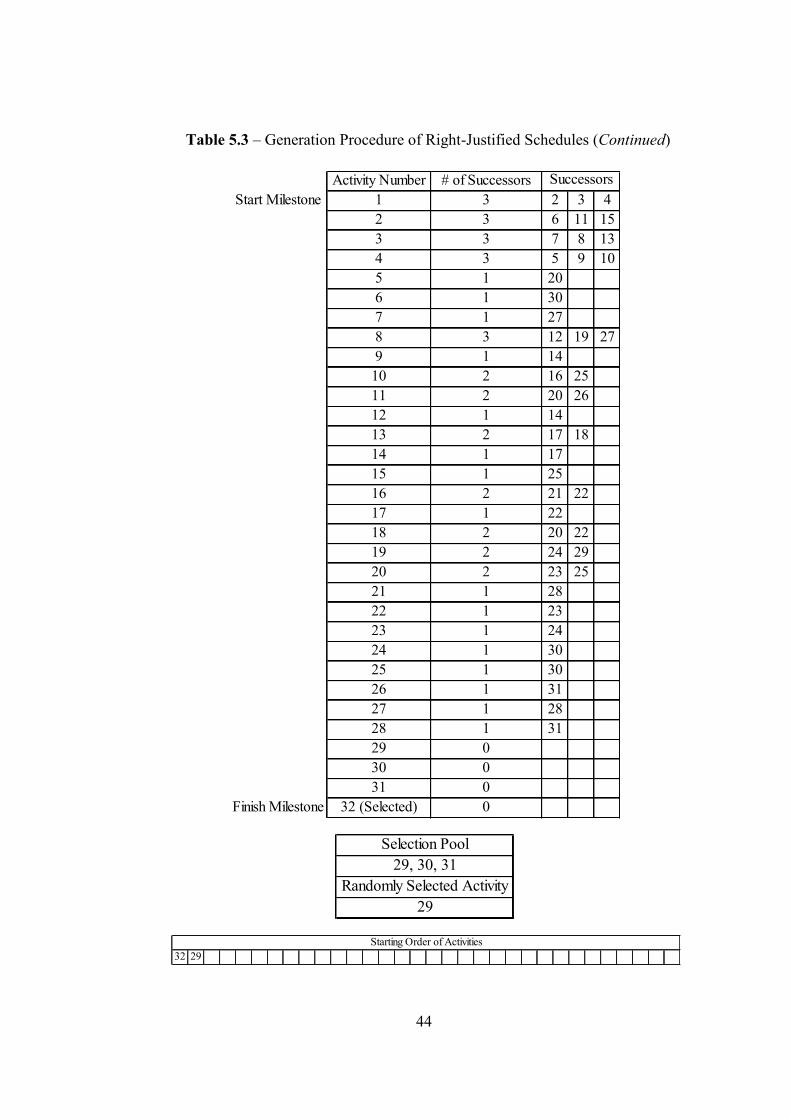
Secondly, left (right) population that is created by using forward (backward)

scheduling. The left (right) population is produced randomly where the

activities with a 0 number of predecessors (successors) are put to the selection

pool and one activity is selected. After this, the numbers of predecessors

(successors) of other activities are recalculated and again the activities with a 0

number of predecessors (successors) are put to the selection pool and one

activity is selected. This cycle is repeated until the finish (start) mile stone has

been started and finally a feasible starting order of activities is found.

39

The first steps of creation of the left and right population are illustrated in

Table 5.2 and 5.3.

Table 5.1 – Conversion of Successor to Predecessor of the Problem

Activity Number # of PredecessorsStart Milestone 1 0

2 1 13 1 14 1 15 1 46 1 27 1 38 1 39 1 4

10 1 411 1 212 1 813 1 314 2 9 1215 1 216 1 1017 2 13 1418 1 1319 1 820 3 5 11 1821 1 1622 2 16 1823 2 20 2224 2 19 2325 3 10 15 2026 1 1127 2 7 828 2 21 2729 1 1930 3 6 24 2531 2 26 28

Finish Milestone 32 3 29 30 31

Predecessors

40

Table 5.2 – Generation Procedure of Left-Justified Schedules

Activity Number # of PredecessorsStart Milestone 1 0

2 1 13 1 14 1 15 1 46 1 27 1 38 1 39 1 410 1 411 1 212 1 813 1 314 2 9 1215 1 216 1 1017 2 13 1418 1 1319 1 820 3 5 11 1821 1 1622 2 16 1823 2 20 2224 2 19 2325 3 10 15 2026 1 1127 2 7 828 2 21 2729 1 1930 3 6 24 2531 2 26 28


Predecessors

Selection Pool1

Randomly Selected Activity1

1Starting Order of Activities

41

Table 5.2 – Generation Procedure of Left-Justified Schedules (Continued)

Activity Number # of PredecessorsStart Milestone 1 (Selected) 0

2 03 04 05 1 46 1 27 1 38 1 39 1 4

10 1 411 1 212 1 813 1 314 2 9 1215 1 216 1 1017 2 13 1418 1 1319 1 820 3 5 11 1821 1 1622 2 16 1823 2 20 2224 2 19 2325 3 10 15 2026 1 1127 2 7 828 2 21 2729 1 1930 3 6 24 2531 2 26 28


Predecessors

Selection Pool2, 3, 4


1 3Starting Order of Activities

42

Table 5.2 – Generation Procedure of Left-Justified Schedules (Continued)

Activity Number # of PredecessorsStart Milestone 1 (Selected) 0

2 03 (Selected) 0

4 05 1 46 1 27 08 09 1 4

10 1 411 1 212 1 813 014 2 9 1215 1 216 1 1017 2 13 1418 1 1319 1 820 3 5 11 1821 1 1622 2 16 1823 2 20 2224 2 19 2325 3 10 15 2026 1 1127 2 7 828 2 21 2729 1 1930 3 6 24 2531 2 26 28


Predecessors

Selection Pool2, 4, 7, 8 13


1 3 8Starting Order of Activities

43

Table 5.3 – Generation Procedure of Right-Justified Schedules

Activity Number # of SuccessorsStart Milestone 1 3 2 3 4

2 3 6 11 153 3 7 8 134 3 5 9 105 1 206 1 307 1 278 3 12 19 279 1 14

10 2 16 2511 2 20 2612 1 1413 2 17 1814 1 1715 1 2516 2 21 2217 1 2218 2 20 2219 2 24 2920 2 23 2521 1 2822 1 2323 1 2424 1 3025 1 3026 1 3127 1 2828 1 3129 1 3230 1 3231 1 32

Finish Milestone 32 0

Successors

Selection Pool32


32Starting Order of Activities

44

Table 5.3 – Generation Procedure of Right-Justified Schedules (Continued)


2 3 6 11 153 3 7 8 134 3 5 9 105 1 206 1 307 1 278 3 12 19 279 1 14

10 2 16 2511 2 20 2612 1 1413 2 17 1814 1 1715 1 2516 2 21 2217 1 2218 2 20 2219 2 24 2920 2 23 2521 1 2822 1 2323 1 2424 1 3025 1 3026 1 3127 1 2828 1 3129 030 031 0

Finish Milestone 32 (Selected) 0

Successors

Selection Pool29, 30, 31


32 29Starting Order of Activities

45

Table 5.3 – Generation Procedure of Right-Justified Schedules (Continued)


2 3 6 11 153 3 7 8 134 3 5 9 105 1 206 1 307 1 278 3 12 19 279 1 14

10 2 16 2511 2 20 2612 1 1413 2 17 1814 1 1715 1 2516 2 21 2217 1 2218 2 20 22

19 (Updated) 1 2420 2 23 2521 1 2822 1 2323 1 2424 1 3025 1 3026 1 3127 1 2828 1 31

29 (Selected) 030 031 0

Finish Milestone 32 (Selected) 0

Successors

Selection Pool30, 31


32 29 31Starting Order of Activities

46

As demonstrated in Tables 5.2 and 5.3, 50 left and right populations are

produced. The complete example schedules of previous tables are introduced in

Tables 5.4 and 5.5.

Table 5.4 – Completed Left-Justified Example Schedule

Table 5.5 – Completed Right-Justified Example Schedule

After creating the starting order, the activities’ start time and finish time can be

calculated. The activities are started by following starting order at first feasible

time according to their resource usage and the resource constraints in the

project.

For the left population, the start milestone can start immediately because it

doesn’t have any predecessor and the activity’s resource requirement is 0.

Therefore, the next activity in starting order is activity 3. The activity 3 has a

predecessor of start milestone and the start milestone is started and finished at

time of 0 and the activity 3 needs a 1st resource of 10. So, the activity 3 can

start at time of 0 and finish at time of 4. Next, in the starting order list, there is

an activity 8. The activity 8 has a predecessor of 3, so the activity 8 can start

after the activity 3 has finished. In addition the activity 8 requires a 2nd

resource of 1 and the activity 8 can start at time of 4 and finish at time of 13

which is the activity’s duration and the activity’s start time. Next in the starting

order list there is an activity 7, the activity 7 has a predecessor of 3, so the

activity 7 can start after the activity 3 has finished. In addition the activity 7

requires a 1st resource of 4 and the activity 7 can start at time of 4 and finish at

time of 9 which is the activity’s duration (5) and the activity’s start time (4) as

illustrated in Figure 5.3.

1 3 8 7 27 2 4 5 12 6 11 9 10 26 15 13 18 16 21 19 14 22 20 17 28 25 31 23 24 30 29 32Starting Order of Activities

32 29 31 28 30 24 26 25 21 23 19 27 20 15 11 6 5 22 17 16 18 13 14 10 12 9 8 7 3 2 4 1Starting Order of Activities

47

Figure 5.3 – Assigning the Left-Justified Schedule Start Time

Figure 5.3 – Assigning the Left-Justified Schedule Start Time (Continued)

During assignment of activities start time and finish time, the precedence

relations and resource usages should be considered. The activity should start

immediately after its precedence is finished if there is an enough resource

throughout the activity’s duration. On the other hand, if the activity has no

predecessor but the resource is inadequate or the resource is available only for

a few days, the activity can be started first resource available day in Figure 5.4.

1211109876543210 1 2 3 4 5 6 7 8 9 10 11 12 13

7

R13

Resource Usage

Time

13121110

9876543210 1 2 3 4 5 6 7 8 9 10 11 12 13

R2

Time8

Resource Usage

48

Figure 5.4 – Completed Left-Justified Schedule of Example Problem

Figure 5.4 – Completed Left-Justified Schedule of Example Problem (Continued)

121110

9876543210 1 2 3 4 5 6 7 8 9 10 11 12 13 14 15 16 17 18 19 20 21 22 23 24 25 26 27 28 29 30 31 32 33 34 35 36 37 38 39 40 41 42 43 44 45 46 47 48 49 50 51 52 53 54 55 Time

22

25

232 15

37

5

9

13

Resource Usage

R1

13121110

9876543210 1 2 3 4 5 6 7 8 9 10 11 12 13 14 15 16 17 18 19 20 21 22 23 24 25 26 27 28 29 30 31 32 33 34 35 36 37 38 39 40 41 42 43 44 45 46 47 48 49 50 51 52 53 54 55 Time

243029

2028

19

14

11

8

12

R2

Resource Usage

49



43210 1 2 3 4 5 6 7 8 9 10 11 12 13 14 15 16 17 18 19 20 21 22 23 24 25 26 27 28 29 30 31 32 33 34 35 36 37 38 39 40 41 42 43 44 45 46 47 48 49 50 51 52 53 54 55 Time

3126R3

Resource Usage

121110

9876543210 1 2 3 4 5 6 7 8 9 10 11 12 13 14 15 16 17 18 19 20 21 22 23 24 25 26 27 28 29 30 31 32 33 34 35 36 37 38 39 40 41 42 43 44 45 46 47 48 49 50 51 52 53 54 55 Time

1718

16

216

10

27

4

R4

Resource Usage

50

5.3 Parent Selection and Crossover Procedure

After producing 50 left individuals and 50 right individuals, the number of

schedules is revised and the next step is calculation of individuals’ fitness

values to guarantee that the algorithm finds appropriate matches. The fitness

values are calculated with following basic formula.

Fitness Value = 1/individual’s makespan

So, the bigger makespan means lower fitness value and that shows the

individual (schedule) is not good in terms of project makespan because the

objective of the problem is minimizing the project makespan.

After calculating the fitness values of individuals, the population is sorted

according to their fitness values and the bigger fitness value is positioned at the

top of the population as shown in Figure 5.5.

Figure 5.5 – Sorting Mechanism of the Algorithm

10% (5 Schedules)

25 Schedules areSelected Randomly

Current Population

TOP

WORST

51

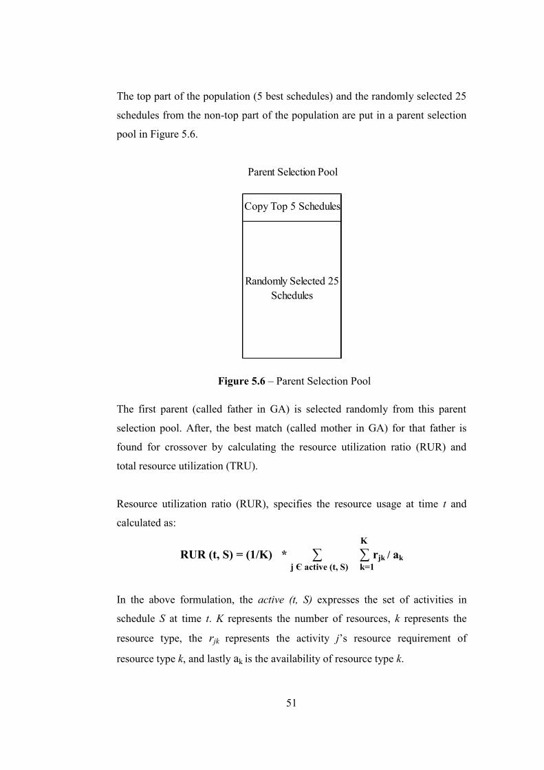
The top part of the population (5 best schedules) and the randomly selected 25

schedules from the non-top part of the population are put in a parent selection

pool in Figure 5.6.

Figure 5.6 – Parent Selection Pool

The first parent (called father in GA) is selected randomly from this parent

selection pool. After, the best match (called mother in GA) for that father is

found for crossover by calculating the resource utilization ratio (RUR) and

total resource utilization (TRU).

Resource utilization ratio (RUR), specifies the resource usage at time t and

calculated as:K

RUR (t, S) = (1/K) * ∑ ∑ rjk / akj Є active (t, S) k=1

In the above formulation, the active (t, S) expresses the set of activities in

schedule S at time t. K represents the number of resources, k represents the

resource type, the rjk represents the activity j’s resource requirement of

resource type k, and lastly ak is the availability of resource type k.

Randomly Selected 25Schedules

Parent Selection Pool

Copy Top 5 Schedules

52

After calculating RUR, the intervals where the resource usages are high and the

intervals where the resource utilization is low will be exposed. In this thesis, t1and t2 are identified as the crossover points where the TRU is maximal between

these points. To that aim, the length of the peak, l is chosen randomly between

(1/4) of makespan and (3/4) of makespan and the total resource utilization of

an interval with a start time t and length l is calculated as:

T+l-1TRU (t, l, S) = ∑ RUR (time, S)

time = t

The crossover point t1 is set to t where t Є [0, makespan-l] for which TRU (t, l,

S) is maximal and the second point t2 is set to t1+l. For the rest of the intervals

the average RUR will be low.

After defining the crossover points according to father, for the remaining

intervals where the RUR is low, the best mother which has a high TRU in

intervals [0, t1] and [t2, makespan] will be found through the parent selection

pool.

Then, two-point crossover operator is applied by using random key (RK)

values of activities. The random key values are used to define the priority list

based on activity information, such as start time or finish time. For left-justified

schedules, the RK takes the value of the finish time of the activity and on the

other hand, in right-justified schedules, the RK takes the value of start time of

the activity and for the child there are 3 cases; in case 1, if mother’s RK<t1, the

child’s RK is mother’s RK–200, in case 2, t1≤ mother’s RK≤ t2, the child’s RK

is father’s RK, and in case 3, if mother’s RK> t2, the child’s RK is mother’s

RK+200.

53

To prevent the ambiguous in priority structure the large constant 200 is used.

Thus, the usage of mother’s best part in terms of resource usage will be

guaranteed.

The example project is taken from (Debels and Vanhoucke, 2007) and the

information, the precedence relations, example schedules of father and mother,

the RUR and TRU profiles, crossover calculations, and the child schedule are

illustrated at Table 5.6, Figure 5.7, 5.8, 5.9, 5.10, Table 5.7, and Figure 5.11,

respectively.

Table 5.6 – Example Project Information for Crossover Operator


The resource availability is 10 for this example project. The colored activities

express the activities which belong to case 2, and hence priority values of

father are same with child’s. In this example, the large constant is taken 50.

Figure 5.7 – Precedence Chart of Example Project for Crossover Operator

A1* A2 A3 A4 A5 A6 A7 A8 A9 A10 A11 A12 A13 A14 A15 A16 A17 A18 A19 A20 A21

*

Duration 0 2 5 8 1 10 9 2 3 8 6 6 9 2 8 6 10 5 8 3 0Resource Usage 0 2 2 6 5 5 3 4 7 3 2 4 4 4 4 1 1 3 2 3 0

1

2

3

4 7

5

15

9 11

12

21

20

8 14 17 18

16

19

6 10 13

54

Figure 5.8 – The Schedule of Father for Crossover

Figure 5.9 – The Schedule of Mother for Crossover

10

9

8

7

6

5

4

3

2

1

0 1 2 3 4 5 6 7 8 9 10 11 12 13 14 15 16 17 18 19 20 21 22 23 24 25 26 27 28 29 30 31 32 33 34 35 36 37 38 39 40 41 42 43 44 45 46 47 48

17

t 1 t 2

11

15

13

18

1619

12

20

2

8

5

14

3

4

Time

Resource Usage

6

7

9

10

10

9

8

7

6

5

4

3

2

1

0 1 2 3 4 5 6 7 8 9 10 11 12 13 14 15 16 17 18 19 20 21 22 23 24 25 26 27 28 29 30 31 32 33 34 35 36 37 38 39 40 41 42 43 44 45 46 47 48

t 1 t 2

2012

16

11

1319

10

159

1718

2

3

8

4

6

714

5

Resource Usage

Time

55

Figure 5.10 – RUR Profile of Father

Table 5.7 – Random Key Values of the Crossover Operator

1.0

0.9

0.8

0.7

0.6

0.5

0.4

0.3

0.2

0.1

0 1 2 3 4 5 6 7 8 9 10 11 12 13 14 15 16 17 18 19 20 21 22 23 24 25 26 27 28 29 30 31 32 33 34 35 36 37 38 39 40 41 42 43 44 45 46 47 48Time

TRU(11, 19, Father) = 16.8

RUR(t, Father)

Activity 1 2 3 4 5 6 7 8 9 10 11 12 13 14 15 16 17 18 19 20 21RK of Father 0 2 5 11 3 21 20 2 24 29 30 43 38 7 32 38 17 37 46 41 46RK of Mother 0 2 5 8 19 18 17 7 30 27 36 43 39 19 27 36 29 34 47 37 47RK of Child -50 -48 -45 -42 3 21 20 -43 24 29 86 93 89 7 32 86 17 84 97 87 97

Child Start Time 0 4 1 0 8 9 10 6 19 19 32 38 27 8 22 30 26 36 36 41 44

56

Figure 5.11 – The Schedule of Child

10

9

8

7

6

5

4

3

2

1

0 1 2 3 4 5 6 7 8 9 10 11 12 13 14 15 16 17 18 19 20 21 22 23 24 25 26 27 28 29 30 31 32 33 34 35 36 37 38 39 40 41 42 43 44 45 46 47 48

12

19

18 207

69

10

13

17

15

16

11

4

3

28

5

14

Time

Resource Usage

57

As shown in Table 5.7, the random key values are activities’ finish time

because father and mother schedules are left-justified schedules. In addition, in

this example, the length of the peak, l is chosen 19, which should be between

(1/4) of makespan which is 11.5 and (3/4) of makespan which is 34.5.

Moreover, the maximum TRU, which is 16.8, is found between 11 and 30 as

seen on Figure 5.10.

Finally, the child schedule is produced. Father and mother schedules were left-

justified schedules, so that the child schedule is right-justified schedule and its

random key values are start time of activities. After crossover operator, the

crossover applied schedules are replaced with randomly selected individuals

from non-top part of the population.

5.4 Mutation Procedure

After crossover operator, the mutation procedure takes place, in proposed

algorithm the mutation rate is %2 which means, just one individual is chosen

from the population. First, one of the schedules is selected randomly from

entire population. Second, one of the activities is selected randomly from the

schedule except start and finish milestones because they are not allowed to

modify. Third, the selected activity’s predecessors’ and successors’ positions

are detected to guarantee that there will be no improper precedence relationship

between activities in the schedule. After, without changing the relations, the

randomly selected activity is shifted with another randomly selected activity.

Then, the makespan of the new schedule is found and the mutation is accepted

if the new makespan is better that previous makespan of the schedule. The

accepted schedule is replaced with the previous schedule. Finally, the schedule

is accepted or not the number of schedules is revised.

58

The previous example will be used to illustrate the mutation operator in Figure

5.12.

Figure 5.12 – Application of Mutation Operator

In the example schedule, the randomly selected activity is 13 and it has a

successor of 19 and the predecessors of 9 and 10. In terms of activity 13’s

precedence constraints, in starting order list, the activities between 10 and 19

are appropriate to replaced with. On the other hand, in terms of activity 15’s

precedence constraints, activity 16 is the successor of activity 15, if this

replacement occurs the activity 15 will be successor of the activity 16 which is

not possible. So, there is only choice to replace activity 13 with activity 16.

1 2 5 3 6 4 7 8 14 9 11 12 10 15 16 13 19 17 18 20 21

9 and 10

The Appropriate Activities to be Replaced with Activity 1316

Activity Starting Order


Successors of Activity 1319

Predecessors of Activity 13

59

CHAPTER 6

COMPUTATIONAL RESULTS

6.1 Computational Results

Throughout the development of this algorithm, some minor changes have been

made in the algorithm and these modified alternatives have been tested on 48

problems with 300 activities. Some of the modifications have outperformed the

first developed algorithm and some of them have a very little effect on GA.

In original algorithm, the father was selected from top population and the

mother was selected from entire population by using the two-tournament

selection where the nominees are chosen randomly from whole population, and

the individual with better (lower) makespan is selected.

In first alternative, 3 schedules have been produced from crossover and other 2

has been added later to the population. In second alternative (final algorithm),

the best mother has been selected thorough 30 individuals. In third alternative,

the top population has not been kept, so the all 30 individuals have been

selected randomly, and in the last alternative, simulated annealing has been

applied during mutation. Results of algorithms are proposed in Table 6.1.

The algorithm’s performance is tested on 480 example problems with 30

activities, 480 example problems with 60 activities, 600 example problems

with 120 activities, and 480 example problems with 300 activities. These

problems can be found on PSPLIB website (http://129.187.106.231/psplib). All

tests have been accomplished by a PC with 12 GB RAM and an Intel Core i7

3.06GH Processing Unit. The computer’s operating system was Windows 7

60

Professional (64 bit) operating system. The results are showed in Table 6.2.

The upper bounds (UB) are the best found solution ever, and lower bounds

(LB) are the CPM durations (without any resource constraints).

Table 6.1 – Computational Results Other Alternatives

Table 6.2 – Computational Results of PSPLIB Problems

Number of Schedules1000

5.26%877.79%

5.20%875.95%

4.80%871.74%

5.21%875.37%

5.00%873.36%

Avg.Dev.Lb

4th Avg.Dev.UbAvg.Dev.Lb

Testing CriteriaAlgorithm

Avg.Dev.UbAvg.Dev.Lb

Original

1st

2nd (final)

3rd



Avg.Dev.Ub

Number of Schedules10001.42%15.35%

3.06%14.65%

8.87%42.62%

4.96%860.25%

Testing CriteriaNumber of Activities


30

60

120

300




61

6.2 Comparison with Primavera Results

Randomly selected 40 problems; 10 problems from each problem sets with 30,

60, 120, and 300 activities have been tested by the algorithm. The selected

problem sets have been also tested by Primavera Project Planner (P6 version

7.0) for comparison. The problems’ CPM lower bounds and upper bounds (best

known solutions) have been known.

The activities are entered to the software with their resource requirements,

durations, and the relations with other activities and scheduled according to

five different algorithms; Activity ID, Total Float, Late Finish, Early Start, and

Free Float. The algorithms are used in both ascending and descending order,

therefore in total 10 algorithms are compared with final algorithm in Table 6.3

and Table 6.4.

According to Primavera results, the Avg. Dev. L.B. and Avg. Dev. U.B. have

been calculated for comparison in Table 6.5, Table 6.6, Table 6.7, and Table

6.8. As seen on tables, in 30 activities, the best solution of Primavera has an

Avg. Dev. L.B. of 84.90% in late finish ascending algorithm while the final

algorithm has an Avg. Dev. L.B. of 64.37%. In 60 activities, the best solution

of Primavera has an Avg. Dev. L.B. of 90.89% in late finish ascending

algorithm while the final algorithm has an Avg. Dev. L.B. of 66.06%. In 120

activities, the best solution of Primavera has an Avg. Dev. L.B. of 155.63% in

late finish ascending algorithm while the final algorithm has an Avg. Dev. L.B.

of 128.79%. In 300 activities, the best solution of Primavera has an Avg. Dev.

L.B. of 1261.82% in late finish ascending algorithm while the final algorithm

has an Avg. Dev. L.B. of 1231.23%. The final algorithm has obviously

outperformed the Primavera Project Planner software.

62

The MS Project software uses the same algorithms with Primavera’s Total

Float (Ascending) and Activity ID algorithms. Hence, the MS Project 2010

software has not been tested.

The best five Primavera algorithms for solving the RCPSPs with 30 activities

are; Late Finish (Ascending), Total Float (Ascending), Early Start (Ascending),

Free Float (Ascending), and Early Start (Descending), respectively. The best

five Primavera algorithms for solving the RCPSPs with 60 activities are; Late

Finish (Ascending), Early Start (Ascending), Total Float (Ascending), Free

Float (Ascending), and Activity ID (Ascending), respectively. The best five

Primavera algorithms for solving the RCPSPs with 120 activities are; Late


Float (Ascending), and Activity ID (Ascending), respectively. The best five

Primavera algorithms for solving the RCPSPs with 300 activities are; Late


Float (Ascending), and Activity ID (Ascending), respectively.

According to the results, the best algorithm is same for all type of problems

with 30, 60, 120, and 300 activities. Late Finish (Ascending) algorithm

outperforms all other algorithms in Primavera. In addition, among the other

heuristic algorithms in Primavera, the Early Start (Ascending) and Total Float

(Ascending) algorithms perform relatively well.

63

Table 6.3 –Comparison of Makespans (30 and 60 activities)

64

Table 6.4 – Comparison of Makespans (120 and 300 activities)

65

Table 6.5 – Comparison of Deviations from L.B. (30 and 60 activities)

66

Table 6.6 – Comparison of Deviations from L.B. (120 and 300 activities)

67

Table 6.7 – Comparison of Deviations from U.B. (30 and 60 activities)

68

Table 6.8 – Comparison of Deviations from U.B. (120 and 300 activities)

69

6.2.1 T-Test for Controlling the Statistical Significance

The t-test is the most commonly used process for hypothesis control that examines

if the means of two data sets are statistically different from each other. Thus, the

differences between best Primavera algorithm and final algorithm can be checked

easily if the difference is significant or not. The best Primavera algorithm in terms

of Avg. Dev. From L.B. (Late Finish (Ascending)) is selected as a control data in

Table 6.9. The t-test results are showed in Table 6.10.

Table 6.9 – T Test

Activity Number Set LF (Asc.) Proposed Algorithm30 1 68.63 41.18

2 110.00 84.293 70.77 58.464 94.12 79.415 93.33 80.006 88.37 62.797 68.18 50.008 109.09 77.279 64.52 40.32

10 82.00 70.0060 1 105.80 72.46

2 26.15 10.773 55.29 31.764 123.75 91.255 85.14 59.466 85.33 58.677 111.94 80.608 124.36 100.009 91.14 73.42

10 100.00 82.19

T-Test for Avg. Dev. From L.B.

70

Table 6.9 – T Test (Continued)

Table 6.10 – T Test Results

120 1 164.29 141.842 202.06 169.073 259.60 227.274 90.29 63.115 175.00 135.586 98.90 76.927 207.37 177.898 204.27 164.969 91.67 80.83

10 62.81 50.41300 1 397.56 373.17

2 2014.29 1950.003 2121.95 2043.904 3722.50 3727.505 1313.11 1216.396 27.41 25.927 11.79 9.178 41.94 41.859 625.42 611.86

10 2342.19 2312.50

Variable 1 Variable 2Mean 378.22661 352.6437162Variance 583663.51 575861.3443Observations 43 43Pearson Correlation 0.9997309Hypothesized Mean Difference0df 42t Stat 9.1204633P(T<=t) one-tail 8.136E-12t Critical one-tail 1.6819524P(T<=t) two-tail 1.627E-11t Critical two-tail 2.0180817

T-Test: Paired Two Sample for Means

71

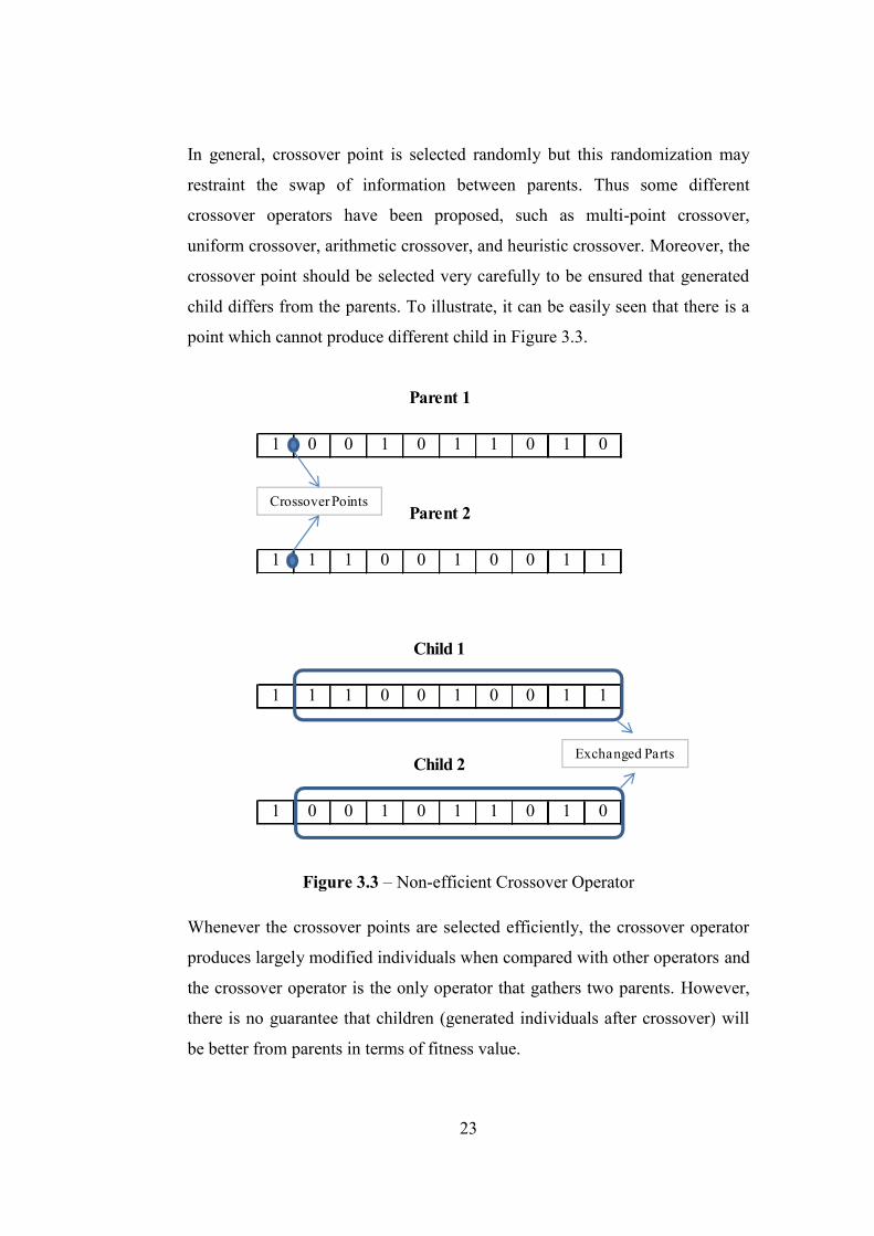
In Table 6.10, the one-tail values will be considered because the final algorithm

outperforms almost all the Primavera results. The t Stat value is found by dividing

the mean of the differences of compared data to standard error. T critical one-tail

is the value is used to decide the significance of differences. As seen on Table

6.10, t Stat value is bigger than t critical one-tail value which means the difference

between Avg. Dev. from L.B. is significant and the small P one-tail value

expresses how critical is it. The P value is very small which shows the significance

is very big between these two data sets. Hence, the final algorithm is significantly

better than the best algorithm of Primavera for the RCPSP.

6.3 Comparison with Published Articles

This final algorithm has been also tested on a few problems in published articles.

The following two problems are taken from (Anagnostopoulos K. and Koulinas

G., 2011).

In first case, there are 15 activities with a resource constraint of 14 and the CPM

solution is 34 days. The MS Project software extends the duration to 71 days and

the proposed algorithm in the (Anagnostopoulos K. and Koulinas G., 2011) and

the final algorithm in this thesis reduces the duration to 54 days, expresses the

23.9% improvement on MS Project’s solution. The network data of the problem,

the initial gantt chart, the best found schedule by their algorithm and the best

found schedule by final algorithm in this thesis are showed in Table 6.11, Figure

6.1, Figure 6.2, and Table 6.12, respectively.

72

Table 6.11 – The Network Data of 1st Case

Figure 6.1 – The Initial Gantt Chart for 1st Case

Activity Name Duration Predecessors Resource DemandA 17 3B 18 3C 17 9D 8 A, C 9E 5 4F 6 2G 7 1H 9 B, D, G 1I 11 B, F 6J 18 E 4K 13 B 4L 3 A 7M 12 A 3N 12 6O 11 2

ProjectDuration

34

73

Figure 6.2 – The Best Found Schedule by Published Article for 1st Case

Table 6.12 – The Best Found Schedule by Final Algorithm for 1st Case

Activity Start Time Finish Time12 41 5414 42 5410 43 549 45 54

11 25 4313 37 4015 25 375 17 253 23 416 18 23

16 7 184 0 172 0 178 30 377 1 7

74

In second case, there are 17 activities with a resource constraint of 6 and the CPM

solution is 126 days. The MS Project software extends the duration to 154 days

and the proposed algorithm in (Anagnostopoulos K. and Koulinas G., 2011) and

the final algorithm in this thesis reduces the duration to 133 days, expresses the

13.63% improvement on MS Project’s solution. The network data of the problem,

the initial gantt chart, the best found schedule by their algorithm and the best

found schedule by final algorithm in this thesis are showed in Table 6.13, Figure

6.3, Figure 6.4, and Table 6.14, respectively.

Table 6.13 – The Network Data of 2nd Case

Activity Name Duration Predecessors Resource Demand0-8 70 1 10-5 33 1 10-2 20 1 11-5 37 1 11-3 40 1 11-6 56 4 12-7 67 4 12-9 78 4 12-8 59 6 13-9 54 6 13-8 54 1 14-6 43 1 14-5 29 1 15-7 37 14, 5, 3 16-9 29 7, 13 17-9 11 15, 8 18-9 32 2, 12, 10 1

ProjectDuration

126

75

Figure 6.3 – The Best Found Schedule by Published Article for 2nd Case

Table 6.14 – The Best Found Schedule by Final Algorithm for 2nd Case

Activity Start Time Finish Time8-9 55 1334-5 101 1336-9 122 1335-7 79 1337-9 55 1223-9 85 1223-8 42 1012-8 47 1014-6 104 1330-5 56 850-8 9 791-3 0 560-2 22 552-9 11 541-6 7 472-7 5 421-5 2 22

76

In another article (Zhang et al., 2006), the permutation-based PSO is proposed to

solve RCPSP and the suggested algorithms are tested in 3 different projects and

the projects networks are presented in Figure 6.4, Figure 6.5, and Figure 6.6,

respectively.

Figure 6.4 – Project Network for the 1st Project

Figure 6.5 – Project Network for the 2nd Project

77

Figure 6.6 – Project Network for the 3rd Project

As seen on previous figures the networks type is activity-on-node and the number

above the node expresses the duration and the numbers below the node are the

resource requirements (usages) of the activities. The resource constraints are

presented in Table 6.15.

Table 6.15 – The Resource Constraints of the Projects

The minimal project durations from different approaches are presented in Table

6.16 and the solution of the projects obtained from the final algorithm in this thesis

are presented in Table 6.17, Table 6.18, and Table 6.19.

78

Table 6.16 – The Project Makespans from Different Approaches

In Table 6.16, the MINAS represent the minimum activity slack (give priority to

one with minimum activity slack, which is computed without considering resource

constraints), the SAD represent the shortest activity duration (give priority to one

with shortest duration), the MILFT represent the minimum late finish time (give

priority to one with minimum late finish time), the GA represents a permutation-

based GA, and the PSO represents the permutation-based particle swarm

optimization (Zhang et al., 2006).

Table 6.17 – The Best Found Schedule by Final Algorithm for 1st Project

In the first project, the best found solution is 15 days in final algorithm in this

thesis. On the other hand, (Zhang et al., 2006) claimed that they obtained the

makespan of 14 days. Thus, the problem is tested again in RESCON software

which provides the exact solution for the RCPSP. The software found the solution

of 15 days too. Therefore, there is an error in (Zhang et al., 2006) in terms of

project makespan. In addition, for the second project our algorithm found the same

solution of 22 with the algorithm in (Zhang et al., 2006), and for the third project

our algorithm found 62 days instead of 61 days that found by (Zhang et al., 2006).

Activity Start Time Finish Time8 9 154 10 157 4 103 6 95 2 66 2 42 0 2

79

Table 6.18 – The Best Found Schedule by Final Algorithm for 2nd Project

Table 6.19 – The Best Found Schedule by Final Algorithm for 3rd Project

Activity Start Time Finish Time2 0 33 0 55 5 74 7 136 7 108 10 149 14 19

10 13 1711 17 197 19 22

12 19 22

Activity Start Time Finish Time2 2 53 5 94 9 128 12 167 16 175 17 2110 21 2215 22 2812 22 256 25 2716 28 3218 32 359 32 3811 35 3820 38 3914 39 4219 42 4623 46 4724 46 5213 47 5017 52 5521 55 5922 55 5926 59 6225 59 62

80

As a result, the final algorithm has found the same result with compared

algorithms; (Anagnostopoulos K. and Koulinas G., 2011) and (Zhang et al., 2006)

in 4 problems. In addition, the final algorithm has found the project duration, one

day more than the solution presented in (Zhang et al., 2006).

81

CHAPTER 7

SUMMARY AND CONCLUSION

In this study, a genetic algorithm for solving resource-constrained project

scheduling problem is proposed. The presented algorithm is capable of solving the

RCPSPs with 30, 60, 120, and 300 activities with 4 different resources. The

algorithm considers constrained resources and activity relationships at the same

time.

In contrast to traditional genetic algorithms, two different initial population are

used, the left population that is produced by forward scheduling and the right

population that is produced by backward scheduling. In doing so, maintaining the

diversity, which is essential part of evolutionary algorithms, has been achieved. In

addition, the probability of crossing over similar population has been disappeared

and the advantages of both forward and backward scheduling have been

harmonized.

Furthermore, modified crossover operator, which is suggested for the first time,

has been used. Advantages of iterative forward/backward scheduling have been

exploited by feeding the left (right)-justified schedules with right (left)-justified

schedules. During this feeding, before crossing over, the population has been

sequenced according to their fitness values and best %10 of the population has

been directly passed to the next generation. In crossover, the parent has been

selected randomly from the parent selection pool and the best partner for the

82

selected parent has been found by using resource utilization ratio and total

resource utilization parameter. The partner schedule is selected according to its

resource utilization. There are two crossover points, so the project makespan has

been divided into three parts. The maximum resource utilization part of the father

has been found and this schedule has been matched with the mother with the

maximum resource utilization in terms of other two parts of the schedule.

Therefore, the father has been paired with the best fit mother in terms of resource

utilization.

After crossing over, lastly, the mutation operator has been used to add entirely new

individual to the population. By accepting the only individuals which have been

improved after mutation, the population is prevented from being worse population.

These processes; crossing over, mutation, and updating the population have been

applied until the maximum number of schedules has been achieved.

Efficiency of the developed algorithm is validated, by comparing the Primavera

results with the results of the final algorithm. 10 problems from each problem sets

with 30, 60, 120, and 300 activities have been solved by both Primavera and final

algorithm. Notwithstanding the number of the activities, the final algorithm is

better than Primavera in the solution of RSPSPs. Moreover, the t-test has been

performed for checking; the differences between Primavera results and the final

algorithm results are significant enough. The t-test result has showed that there is a

considerable difference between solutions. In addition, when the Primavera’s

solutions are compared with the final algorithm, the performance of Primavera is

observed unsatisfactory to solve resource-constrained project scheduling problems.

The performance of the algorithm is also tested by solving resource constrained

project scheduling problems in the literature. Results achieved by the final

83

algorithm are analyzed and compared with the solutions of other researchers. 5

different problems have been solved. Final algorithm solved these problems and

found the reasonably well solutions. In this manner, the capability of the final

algorithm has been proved for these problems.

The performance of the algorithm has been tested using PSPLIB instances. 480

example problems with 30 activities, 480 example problems with 60 activities, 600

example problems with 120 activities, and 480 example problems with 300

activities have been used. The deviations of the algorithm from the best known

solutions are about %1.4 to %8.9. Hence, the final algorithm provided adequate

results.

Within the context of this study, two essential contributions to the existing

researches are made. Firstly, a unique crossover operator has been presented and

used. With the new crossover operator, especially in large projects, the

performance improvement has been observed when compared to conventional

GAs. Secondly, the Primavera software has been tested on small and large projects

with number of activities of 30, 60, 120, and 300 and compared with the final

algorithm. Thus, the performance of developed algorithm has been clearly

observed. In addition to these, the best Primavera algorithm for the RCPSP has

been observed as Late Finish (Ascending) algorithm.

As computational outcomes show, to find better solutions, more CPU time is

required, especially in large-sized projects. Being an iterative algorithm, better

solutions can be reached by using more processing units. Therefore, the

computational performance can be easily increased by using supercomputers,

parallel computing, or graphic based processing units. In addition to the using new

84

technologies, changing code architecture or combining the genetic algorithm with

other meta-heuristic methods can increase the performance of existing study.

85

REFERENCES

Abeyasinghe M. Chelaka L., Greenwood David J., and Johansen D. Eric, (2001).

“An Efficient Method for Scheduling Construction Projects with Resource

Constraints”, International Journal of Project Management, 19:29-45.

Alcaraz J. and Maroto C., (2001). “A Robust Genetic Algorithm for Resource

Allocation in Project Scheduling”, Annals of Operations Research, 102, 83–109.

Alcaraz J., Maroto C., and Ruiz R., (2004). “Improving the performance of genetic

algorithms for the RCPS problem”, Proceedings of the Ninth International

Workshop on Project Management and Scheduling, 40–43.

Anagnostopoulos K. and Koulinas G., (2011). “Resource-Constrained Critical Path

Scheduling by a GRASP Based Hyperheuristic”, Journal of Computing in Civil

Engineering, March.

Artigues C., Demassey S., and Néron E., (2008). “Resource-Constrained Project

Scheduling: Models, algorithms, extensions and applications”, Wiley, Hoboken.

Bent J.A. and Thumann A., (1994). “Project Management for Engineering and

Construction”, The Fairmont Press, Lilburn.

Bettemir Ö.H., (2009). “Optimization of Time-Cost-Resource Trade-off Problems

in Project Scheduling Using Meta-heuristic Algorithms”, Middle East Technical

University, PhD. Dissertation.

86

Blazewicz L., Lenstra J., and Kan A.R., (1983). “Scheduling subject to resource

constraints: classification and complexity”, Discrete Applied Mathematics, 5, 11-

24.

Bouleimen K. and Lecocq H., (2003). “A New Efficient Simulated Annealing

Algorithm for the Resource-Constrained Project Scheduling Problem and Its

Multiple Mode Version”, European Journal of Operational Research, 149:268–

281.

Chen W., Shi Y-J, Teng H-F, Lan X-P, and Hu L-C, (2010). “An Efficient Hybrid

Algorithm for Resource-Constrained Project Scheduling”, Information Sciences,

180:1031–1039.

Christodoulou S., (2010). “Scheduling Resource-Constrained Projects with Ant

Colony Optimization Artificial Agents”, Journal of Computing in Civil

Engineering, January-February, pp. 45-55.

Colak S., Agarwal A., and Erenguc S., (2006). “Resource-Constrained Project

Scheduling Problem: A Hybrid Neural Approach”, Perspectives in Modern Project

Scheduling (Jan Weglarz and Joanna Jozefowska, eds), 297-318.

Debels D., Reyck B., Leus R., and Vanhoucke M., (2004). “A Hybrid Scatter

Search Electromagnetism Meta-Heuristic for Project Scheduling”, European

Journal of Operational Research, 169:638–653.

Debels D. and Vanhoucke M., (2005). “A Bi-Population Based Genetic Algorithm

for the Resource-Constrained Project Scheduling Problem”, Vlerick Leuven Gent

Working Paper Series, 6482/08.

87

Debels D. and Vanhoucke M., (2006). “Meta-Heuristic Resource-Constrained

Project Scheduling: Solution space restrictions and neighbourhood extensions”,

Faculteit Economie en Bedrijfskunde, University Gent, May, 387.

Debels D., Vanhoucke M., (2007). “A Decomposition-Based Genetic Algorithm

for the Resource-Constrained Project-Scheduling Problem”, Operations Research,

Vol. 55, No. 3, May–June, pp. 457–469.

Demeulemeester E.L. and Herroelen W.S., (2002). “Project Scheduling: A

Research Handbook”, Kluwer Academic Publishers, Boston.

Franco E.G., Zurita F.T., and Delgadillo G.M., (2007). “A Genetic Algorithm for

the Resource Constrained Project Scheduling Problem (RSPSP)”,

Bolivia Research and Development, Vol. 7, pp. 41 – 52.

Hartmann S., (1998). “A Competitive Genetic Algorithm for Resource-

Constrained Project Scheduling”, Naval Research Logistics, 45:733-750.

Hong W., Tongling L., and Dan L., (2010). “Efficient Genetic Algorithm for

Resource-Constrained Project Scheduling Problem”, Transactions of Tianjin

University, 16: 376-382.

Kim K., (2003). “A Resource-constrained CPM (RCPM) Scheduling and Control

Technique with Multiple Calendars”, Virginia Polytechnic Institute and State

University, PhD. Dissertation.

88

Kim J-L, and Ellis R.D., (2008). “Permutation-Based Elitist Genetic Algorithm for

Optimization of Large-Sized Resource-Constrained Project Scheduling”, Journal

of Construction Engineering and Management, November, pp. 904-913.

Kochetov Yu.A. and Stolyar A.A., (2003). “Evolutionary Local Search with

Variable Neighborhood for the Resource Constrained Project Scheduling

Problem”, Workshop on Computer Science and Information Technologies (CSIT),

Ufa, Russia.

Kolisch R. and Hartmann S., (2006). “Experimental Investigation of Heuristics for

Resource-Constrained Project Scheduling an Update”, European Journal of

Operational Research, 174:23–37.

Leu S-S, Chen A-T, and Yang C-H, (1999). “Fuzzy Optimal Model for Resource-

Constrained Construction Scheduling”, Journal of Computing in Civil

Engineering, July, pp. 207-216.

Mendes J.J.M., Goncalves J.F., and Resende M.G.C., (2005). “A Random Key

Based Genetic Algorithm For the Resource Constrained Project Scheduling

Problem”, June, AT&T Labs Research Technical Report.

Mobini M.D.M., Rabbani M., Amalnik M.S., Razmi J., and Rahimi-Vahed A.R.,

(2009). “Using an Enhanced Scatter Search Algorithm for a Resource-Constrained

Project Scheduling Problem”, Soft Comput, 13:597–610.

Mobini M., Mobini Z., and Rabbani M., (2010). “An Artificial Immune Algorithm

for the Project Scheduling Problem Under Resource Constraints”, Applied Soft

Computing Journal, pp. 1975-1982.

89

Mutlu M.Ç., (2010). “A Branch and Bound Algorithm for Resource Leveling

Problem”, Middle East Technical University, M.Sc. Thesis.

Ranjbar M., (2008). “Solving the Resource-Constrained Project Scheduling

Problem Using Filter-and-Fan Approach”, Applied Mathematics and Computation,

201:313–318.

Seda M., Matousek R., Osmera P., Pivonka P. and Sandera C., (2009). “A Flexible

Heuristic Algorithm for Resource-Constrained Project Scheduling”, Proceedings

of the World Congress on Engineering and Computer Science, October, Vol 2.

Thomas P.R. and Salhi S., (1998). “A Tabu Search Approach for the Resource

Constrained Project Scheduling Problem”, Journal of Heuristics, 4: 123–139.

Toklu Y. Cengiz, (2002). “Application of Genetic Algorithms to Construction

Scheduling with or without Resource Constraints”, Canadian Journal of Civil

Engineering, 29: 421–429.

Torres J.R.M., Franco E.G., and Mayorga C.P., (2010). “Project Scheduling with

Limited Resources Using a Genetic Algorithm”, International Journal of Project

Management, 28:619–628.

Tseng L-Y and Chen S-C, (2006). “A Hybrid Metaheuristic for the Resource-

Constrained Project Scheduling Problem”, European Journal of Operational

Research 175:707–721.

90

Valls V., Ballestin F., and Quintanilla S., (2003). “A hybrid genetic algorithm for

the RCPSP”, Technical report, Department of Statistics and Operations Research,

University of Valencia.

Valls V., Ballestin F., and Quintanilla S., (2004). “A population-based approach to

the resource-constrained project scheduling problem”, Annals of Operations

Research, 131:305–324.

Valls V., Ballestin F., and Quintanilla S., (2005). “Justification and RCPSP-A

Technique That Pays”, European Journal of Operational Research, 165:375–386.

Valls V., Ballestin F., and Quintanilla S., (2008). “A Hybrid Genetic Algorithm

for the Resource-Constrained Project Scheduling Problem”, European Journal of

Operational Research, 185:495–508.

Wall M.B., (1996). “A Genetic Algorithm for Resource-Constrained Scheduling”,

Massachusetts Institute of Technology, PhD. Dissertation.

Xiaoguang Y., Dechen Z., Lanshun N., and Xiaofei X., (2009). “A Novel Genetic

Simulated Annealing Algorithm for the Resource Constrained Project Scheduling

Problem”, Institute of Electrical and Electronics Engineers, May, 978-1-4244-

3894.

Zhang H., Li H., and Tam C.M., (2006). “Particle Swarm Optimization for

Resource-Constrained Project Scheduling”, International Journal of Project

Management, 24:83–92.

91

Zhang H., Li H., and Tam C.M., (2006). “Permutation-Based Particle Swarm

Optimization for Resource-Constrained Project Scheduling”, Journal of

Computing in Civil Engineering, March-April, pp. 141-149.

Date post:	16-May-2018
Category:	Documents
Upload:	ngonhi
View:	213 times
Download:	0 times

A GENETIC ALGORITHM FOR THE RESOURCE CONSTRAINED PROJECT SCHEDULING PROBLEM...

Documents