DEPARTMENT OF ECONOMICS WORKING PAPER SERIES

A Global Analysis of Income Distribution and Capacity Utilization

Interactions: The Structuralist View

Tanadej Vechsuruck

Working Paper No: 2017-08

November 2017

University of Utah

Department of Economics

260 S. Central Campus Dr., Rm. 343

Tel: (801) 581-7481

Fax: (801) 585-5649

http://www.econ.utah.edu

A Global Analysis of Income Distribution and Capacity Utilization Interactions:

The Structuralist View

Tanadej Vechsuruck University of Utah

e-mail u0702590@utah.edu

Abstract

The demand and distributive regimes are estimated from 62 countries around the world

based on the Structuralist Goodwin model. The distributive regime appears to be

Marxian/profit-squeeze and the demand exhibits a weekly profit-led regime. The profit-

led demand regime and the profit-squeeze distributive regime are stronger in advanced

economies than in emerging economies. The results are also supported when the slopes

are allowed to be varied across regions. In the long run, the results reveal that the

collective wage suppression would result only in declining wage share, and no positive

gain in utilization is found both in developed and developing countries.

Keywords: Panel Analysis, Predator-Prey Models, Distributive-Demand Dynamics,

Globalization

JEL Classification: C23, D3, O11, O47

A Global Analysis of Income Distribution and CapacityUtilization Interactions: The Structuralist View

Tanadej Pete Vechsuruck∗

November 15, 2017

Abstract

The demand and distributive regimes are estimated from 62 countries around theworld based on the Structuralist Goodwin model. The distributive regime appears tobe Marxian/profit-squeeze and the demand exhibits a weekly profit-led regime. Theprofit-led demand regime and the profit-squeeze distributive regime are stronger inadvanced economies than in emerging economies.The results are also supported whenthe slopes are allowed to be varied across regions. In the long run, the results revealthat the collective wage suppression would result only in declining wage share, and nopositive gain in utilization is found both in developed and developing countries.

Keywords: Panel Analysis, Predator-Prey Models, Distributive-Demand Dynamics,Globalization

JEL Codes: C23, D3, O11, O47

∗Department of Economics, University of Utah

1 Introduction

Inequality has recently become one of the greatest concerns for economic scholars. Sev-eral books have discussed the possible causes as well as the consequences and solutions (seeAtkinson (2015), Piketty (2014), Milanovic (2005) among several others). Many internationalorganizations have also investigated the issue in different dimensions (see UNCTAD (2012)and IMF (2017) for example). Similar to many other issues in the macroeconomic field, thereis no consensus on the main cause of inequality. The causes can range from skill-biased tech-nological change, international trade and capital account openness to financialization. Thereare many different ways to look at inequality. Functional income distribution, the incomeshares between capital and labor, is considered as the measure that has gained popularity inthe past few years, since many studies have found wage share trends in several economies.

In particular, several studies have shown that the labor share in many developed anddeveloping countries has fallen since the 1980s, although the causes are still controversial(see Stockhammer (2013) among others). This phenomenon is in contrast to one of Kaldor’sstylized facts (Kaldor, 1957), which argued that the income share between labor and capitalshould be constant across time. The stability of the income shares is very crucial sinceit has been one of the main pillars of Neoclassical macroeconomics. For the neoclassicalmacroeconomics model, the shares of income should be constant because if wages becomehigher, firms should invest in more machines, and vice versa. The substitution between thetwo inputs should therefore stabilize the factor shares of income. When the shares are notstable, why the substitution does not work needs to be clarified. For instance, a declinein labor share might be explained by the decline of the relative price of investment goods(Karabarbounis and Neiman, 2013).

For post-Keynesian macroeconomics, the period of stability between wage and profitshares can be viewed as a temporary balance of social conflict, given the set of economicand political configurations. The income share fluctuation, according to the theory, createsfluctuations for demand components: consumption, investment and net exports. If theeconomy is demand-driven, instability in income shares can also create economic fluctuations.Thus, when the wage share falls in a certain economy, demand can be increased or decreaseddepending on how each component reacts. The total effect is therefore an empirical question.How does the wage share instability create a business cycle? At the international level, arethe characteristics of business cycles in developed and developing countries similar? If not,what are the differences and what do they imply? In the long run, does the global economygain from the instability of the wage share? If not, what are the possible explanations?

This study is intended to answer these questions. The Structuralist Goodwin model willbe adjusted and empirically tested on the unbalanced panel data of 62 countries. Althoughmany empirical studies have examined many different developed countries, only some studieshave included developing countries. This study will compare and contrast the results between

1

regions and countries both in the short run and long run.

The structure of this study is the following. After the Introduction (1), the TheoreticalModel section (2) will explain the construction of Structuralist Goodwin model. The thirdsection, Empirical Analysis (3), will be separated into three subsections. The first subsection,Wage Share and Capacity Utilization data (3.1), will clarify how main variables data aregathered and adjusted for the study. The second subsection, Panel Data Analysis (3.2),will explain the econometric models this study is based on and analyze the findings. Thethird subsection, Discussion:the Global Beggar-My-Neighbor Game (3.3), will consider theimplications of the results. Finally, the last part, Conclusion (4), will summarize the essenceof this work and elaborate some concerns.

2 The Structuralist Goodwin Model

Following Marx’s idea on social conflict (Marx, 1867) and the Lotka-Volterra mathemat-ical model (Lotka, 1925) on the competition between species, Goodwin (1967) constructeda macroeconomic model to show that a business cycle can be explained by two endogenousvariables: income distribution, or the predator, and employment, or the prey. In his model,Say’s law is assumed as saving determines investment and an economy always operates atfull capacity, which implies a constant capital-output ratio. A distributional conflict betweenlabor and capital is shown along with the dynamics between wage share and employmentratio. Hirsch and Smale (1974, pp. 262) showed that with the construction of the system’sJacobian matrix, the main diagonal elements appear to be all zeros, which creates a closedorbit–the dynamics of wage share and employment ratio chasing each other in a counter-clockwise fashion. The business cycle is inherently started when employment (the prey) andwage share (the Predator) increase. As the wage share rises, it simultaneously decreases theprofit share, economic growth, capital accumulation, and thus employment. The Goodwincycle is therefore generated by only two conflicting endogenous variables.

Based on the literature from Keynes (1936), Kalecki (1971) and Steindl (1952), a num-ber of post-Keynesian macroeconomists, including Bhaduri and Marglin (1990), Dutt (1984),Taylor (1991), Rowthorn (1981), Foley and Michl (1999) and Blecker (1989), among others,have developed Keynesian economic growth theory in which effective demand is emphasizedas key to economic growth. The importance of income distribution is revived along thelines of classical economics dating back to Smith, Ricardo and Marx. The StructuralistGoodwin model presented below closely follows the business cycle model developed in N. H.Barbosa-Filho (2001), N. Barbosa-Filho and Taylor (2006) and Taylor (2004) in which in-come distribution and capacity utilization are endogenized. In particular, this heterodoxbusiness cycle model incorporates effective demand into social conflict in order to examinehow income distribution interacts with business fluctuations. The concept of distribution-demand interactions was also further scrutinized in a non-linear fashion. Tavani et al. (2011)

2

propose that with a non-linear distributive curve that allows for both forced-saving andprofit-squeeze in the system and profit-led demand curve, the US economy could have threeequilibria corresponding to different rates of wage share and capacity utilization. Nikiforosand Foley (2012) show that with the U-shaped distributive curve, the economy might bestuck in a low equilibrium trap. Even though the whole demand regime is profit-led, thestate of multiequilibria suggests that the low-level equilibrium can be reconsidered as wage-led and a redistribution toward labor at that point would improve the economy.

The Structuralist Goodwin model is fundamentally composed of two regimes: the de-mand regime and the distributive regime. The demand regime captures the causal effectfrom income distribution to effective demand. In a closed economy without government,the demand regime is considered profit-led 1 when a positive effect of higher profit shareon investment dominates the negative effect of higher profit share on consumption. Theopposite case is called wage-led when the positive effect of higher wage share on consump-tion is large enough to offset the negative effect of higher wage share on investment. Thedistributive regime, on the other hand, captures the causal effect from effective demand toincome distribution. The distributive regime could also act in two main ways. If increasingeconomic activity causes a negative effect on wage share, we say the distributive regime iswage-squeeze, forced-saving, or Kaldorian.2 However, if higher demand, which usually causeslower unemployment, lifts the bargaining power of labor and leads to a rising wage share,the distributive regime is labeled as profit-squeeze or Marxian. Next, the theoretical modelwill be analyzed in detail and its possible ‘closures’ (for more details, see Taylor (1991, pp.41)) determined by different technological levels, labor market structures and institutionsacross economies.

Suppose a closed economy produces only one good and a government has no role. Asociety is divided into two classes: capitalists whose income is mainly derived from profitand workers whose income is mainly derived from wage. Capacity utilization (u) is definedas real output (X) over existing capital or potential output (K). Wage share (ψ) is definedas real wage (ω) over labor productivity (ξ). By differentiating u and ψ with respect to time(given that x = x

xwhen x is continually differentiable), we have

u = X − K (1)

ψ = ω − ξ (2)

The growth rate of utilization relies on the difference between growth rates of output and

1Suppose the total income is separated into wage and profit. The sum of the wage share and the profitshare must equal one. The profit-led/wage-led definition was coined by Taylor (1991), while the meaning iscomparable to the terms in Bhaduri and Marglin (1990), exhilarationist/stagnationist, respectively.

2Kaldor (1956) hypothesizes that an economy needs to shift distribution in favor of capitalists during thebooming period, so they can have sufficient funds to make investments in the following period. Marx, onthe other hand, emphasizes the role of the reserve army of unemployed that makes labor’s bargaining power,and thus real wage, vary pro-cyclically.

3

capital (suppose there is no capital depreciation) while the growth rate of wage share isthe difference of real wage growth and labor productivity growth. The relationship betweenutilization and wage share can be further scrutinized by using the Two-Species Model (formore details, see Shone (2002, chapter 14) since they can be thought of as two species that canbe rivalry or predatory. Output, capital, real wage and labor productivity are constructedas a linear function consisting of our two species: utilization and wage share as follows,

X = α0 + αuu+ αψψ (3)

K = β0 + βuu+ βψψ (4)

ω = γ0 + γuu+ γψψ (5)

ξ = δ0 + δuu+ δψψ (6)

Then equation (3) and equation (4) are substituted into equation (1) and equation (5) andequation (6) are substituted in equation (2). Also, let φj = αj − βj and θj = γj − δj forj = 0, u or ψ. We can obtain

u = u(φ0 + φuu+ φψψ) (7)

ψ = ψ(θ0 + θuu+ θψψ) (8)

Equation (7) and equation (8) can be constructed as the utilization nullcline and distributivenullcline, respectively, after they are equated to zero. The stationary solution, the long-runsolution and the stability analysis are elaborated in Appendix A. The slope of utilizationnullcline depends on the sign of φψ or the difference between the effects of wage sharechanges on output and capital. When the sign of φψ is positive, the utilization nullcline ispositively sloped or the demand regime is wage-led. The negative φψ causes the utilizationnullcline to be negatively sloped or the demand regime is profit-led. The slope of distributivenullcline, on the other hand, largely rests on the sign of θu or the difference between theeffects of utilization changes on real wage and labor productivity. The positive θu resultsin a positively sloped distributive nullcline or the distributive regime is profit-squeeze. Thedistributive regime is considered as wage-squeeze when θu is negative, which causes the slopeof the distributive nullcline to be negative as well.

Figure 1 illustrates the system with profit-squeeze distributive and profit-led utilizationregimes. The system manifests counter-clockwise predator-prey dynamics, where the wageshare is a predator and capacity utilization is a prey. At the beginning of the businesscycle, a reduction in the wage share induces a higher investment that overshadows a fallin consumption. An increase in capacity utilization strengthens the bargaining power oflabor that eventually leads to a higher labor share. This would set the stage for an economicslowdown and the cycle would come to an end. The new cycle will start when a lowering wageshare stimulates the aggregate demand again. The dynamic behavior can be characterizedas ‘spiral sink’ as it converges to the long-run equilibrium. In this system, a pro-labordistributive shock, or a leftward shift of the distributive nullcline, will improve the wage

4

share while worsening utilization. A positive demand shock, or a rightward shift of theutilization schedule, will improve both wage share and utilization in this system.

Wage-led and wage-squeeze dynamics regimes are shown in Figure 2 . The systemexhibits clockwise predator-prey dynamics where a predator is instead performed by capacityutilization while wage share turns out to be a prey. The business cycle starts when theeconomy is boosted by an increase in wage share. Higher consumption is large enough tocompensate for a reduction in investment. The economy expands until the profit share startsto increase. The period of recession stalls the economy until the wage share begins to riseagain and the new cycle begins. Likewise, the dynamic behavior is still considered as ‘spiralsink’. Nevertheless, a pro-labor shock in this system will improve both labor share andutilization, whereas a positive demand shock will improve only utilization but discouragelabor share.

In Figure 3, the distributive curve shows the forced-saving/Kaldorian characteristicwith the profit-led demand regime. In this case, the distributive schedule must cut thedemand schedule from above to make the system stable (Taylor, 2004). In other words,the distributive schedule must be steeper than the demand schedule in order to have apositive determinant for the Jacobian matrix. As a result, the system also embraces counter-clockwise predator-prey, spiral-sink dynamics, as in the first case. However, while a pro-labordistributive shock causes the same effect as the case above, a positive demand shock willsuffer the wage share in this case.

Economic structures, market characteristics and social institutions fundamentally de-termine the nature of distributive and demand regimes in each economy. Due to rapidglobalization in the past few decades, many economists may expect the regime to be verysimilar across developed and developing countries. Even though we have seen evidence thatmany countries have tried to capture the benefit of globalized markets of goods and servicesby suppressing labor renumeration, how an economy reacts across a business cycle shall beleft for empirical analysis. In the next section, the panel data analysis is utilized in orderto see how the distributive and demand regimes look in developed and developing countries.Similarities and differences of the regimes will also be discussed between different groups ofcountries.

3 Empirical Analysis

This section will translate the Structuralist Goodwin model described earlier into theempirical model.

5

3.1 Wage Share and Capacity Utilization Data

Regarding the theoretical model above, we recognize that any econometric model thatattempts to empirically test the Structuralist Goodwin model requires two endogenous vari-ables’ time series data, namely wage share and capacity utilization. The two variables aredefined below.

First of all, capacity utilization cannot be defined straightforwardly as in the model.Although effective output is generally defined as the current GDP, difficulty exists in howto measure capital or potential output. In this study, capacity utilization is defined as theGDP gap, which is calculated by the percentage difference between actual (or effective) andpotential GDP. The actual real GDP is measured at the 2005 constant local currency. Allactual real GDP data are gathered from “National Accounts Estimates of Main Aggregates”from the United Nations Statistics Division (UNSD). Potential output is obtained from thestandard Hodrick-Prescott (HP) filter with a smoothing parameter of 100 because the dataare in the annual level. The idea of this statistical filter is simply to separate cyclical fromstructural components of actual GDP.

Far from uncontroversial, the HP filter has been criticized in the past few years. Cogleyand Nason (1995) claim that the HP filter can potentially create spurious cycles. In addition,Hamilton (2017), while agreeing that the HP filter generally produces series with spuriousdynamics relations, argues that the spurious dynamics, created by the filter, also makefiltered values at each end of the sample very different from those in the middle. Blecker(2016) compares US utilization rates obtained from the HP filter and from a survey by USfirms. He found that the utilization from the HP filter downplays the adverse effect from the2008 financial crisis. Also, the HP filter fails to show the downward trend in utilization, asshown in the survey. Be that as it may, the HP filter is still considered to be one of the mostconventional filters and most suitable to apply here because the data are collected annuallyand considered not rich in terms of their lengths and numbers of observations.

Wage share is defined as compensation of employee over gross value added. All dataare collected from “National Accounts Official Data” Table 2.3 at UNSD, except data fromChina and Taiwan.3 The wage share index is calculated as the current wage share overthe 2005 wage share times a hundred. The index transformation allows us to compare thechanges in wage share across time and location, considering the fact that absolute values arevery different across countries.

How to calculate wage share is still far from conclusive especially in developing countrieswhere labor markets are rampant with informal employment. In many emerging economies,a majority of the labor force works in unincorporated enterprises. Income data from such

3Chinese data from 1978-1995 are received from Li (1999). Afterwards, China Statistical Yearbook,published by the National Bureau of Statistics of China, provides all the data. Data for Taiwan are gatheredfrom National Statistics (Republic of China (Taiwan)).

6

employment are difficult to record in national income account categories. Most countries,for a variety of reasons, just record the self-employed as capital income, so the size of wageshare is underestimated. Gollin (2002) proposes an alternative methodology to deal with thisissue by correcting the underestimation of unincorporated enterprises. Onaran and Galanis(2012) follow the methodology to deal with developing countries’ wage shares but substitutedoperating surplus of Private Unincorporated Enterprise (OSPUE) with mixed income. Theproblem with the UN data we have is that the mixed income data are not consistent withthe wage share data. There are only three developing countries (Brazil, Iran and Mongolia)that have the length of mixed income data equal to wage share data, whereas others havea shorter length of mixed income data or none at all. Moreover, it is very likely that theadjustment changes only the absolute values of wage share, not relative values. Figure 4shows a comparison between the original and adjusted wage share for Brazil.4 It clearlyshows that the adjustment does not change the trend at any time and the size of mixedincome seems to be constant throughout the time period, namely a constant gap betweenthe original and adjusted wage shares. Therefore, we assume that the size of mixed incomerelative to total income is constant for all countries across time. The original wage shareindex is chosen to be estimated for all countries. 5

Tables 1 and 2 summarize the list of countries, two main variables, and the period ofdata availability for each country. Overall, there are 62 countries from all regions around theworld. Countries are selected if they have data available for constructing two indexes after1970 and until 2014. Most countries have perfect data to construct the GDP gap during theperiod 1970-2014.6 Unfortunately, only a handful of countries have the full range of datafor wage share while most countries have different ranges, from more than 30 years to only15 years. Countries are classified as developed or developing based on the pre-crisis reportfrom IMF (2008) except that the Asian Tigers (Hong Kong, Singapore, South Korea andTaiwan) and Israel are categorized as developing countries because they were classified asdeveloped countries only recently, in 1997. In addition, heavily indebted poor countries areexcluded from developing countries in order to have a group of countries less variation inincome levels. The post-Soviet states are also excluded as the collapse of the Soviet Unionmade the wage share highly volatile in the early 1990s.

4Here the adjustment method in Onaran and Galanis (2012) is used. The adjusted wage share equalsthe average of the two methods. The first method applies the definition that adjusted wage share equalsto (compensation of employee + mixed income)/(gross value added) while the second method defines theadjusted wage share equals (compensation of employee)/(gross value added - mixed income). These twomethods are not perfect in themselves. The first method might overstate the size of labor income as itincorporates all the mixed income in labor compensation. The second method is only plausible under theassumption that an unincorporated enterprise has the same proportion of income as the rest of the economy.The average of the two methods is therefore applied.

5Additionally, the Chinese data have already been adjusted for OSPUE several times in the past fewyears. See Zhou et al. (2010) and Qi (2014) for more details.

6Note that the full range of real GDP 1970-2014 is used to create the series of potential output for allcountries despite the fact that not all numbers are used since the wage share indexes for many countries areshorter.

7

Figures 5, 6, 7 and 8 reveal some interesting trends in wage share across the globe.While most countries have inconclusive or stable trends, there are many countries whosewage share trends are very clear, i.e., increasing or decreasing. In agreement with manystudies before, several countries around the world have suffered from falling wage sharetrends. Among developed countries, Figure 5 shows that wage shares in Australia, Canada,Germany, Ireland, Italy, the Netherlands, Norway, Sweden, the US and the UK have hadstark falling trends since the 1970s . Only Denmark and Iceland have increasing trends asshown in Figure 6. Iceland’s wage share has rapidly increased since 1984 after it had declinedfor a decade. Denmark’s wage share, although the trend seems stable during the 1970s to1990s, has gradually increased since the mid 2000s.

In developing countries, the big picture is very similar: only a couple of countries haveincreasing trends whereas many countries have declining trends. In Figure 7 , China, Peru,Mauritius, South Africa, Taiwan and Venezuela have falling wage share trends for the pastfew decades. On the contrary, wage shares in South Korea and Thailand, as shown in Figure8, have increased over time since the 1970s but became stable after the Asian Financial Crisisin 1997. It should be noted that the Asian Tigers (Hong Kong, Taiwan, Singapore and SouthKorea) plus China and Thailand, countries that have rapidly grown since the 1970s, haveexperienced differently in terms of wage share trends. While South Korea and Thailand’ shave significantly rising trends, as argued above, Taiwan and China have dramatically fallingtrends.

3.2 Panel Data Analysis

After several theoretical works published since the early 1990s, a sizable number of em-pirical literature have followed by investigating how changes in income distribution betweenwage and profit earners have a quantitative effect on the demand regime. According toBlecker (2016), those empirical studies can be approximately separated into two categories.The first category is called the ‘structural approach’. Most studies in this category applieda single equation method to measure the partial effects of consumption, investment andnet exports to wage share (or profit share). Whether the open-economy demand regime iswage-led or profit-led is calculated from the sum of all partial effects. For the close-economydemand regime, the calculation merely disregards the net exports effect. Until now, theempirical results have been inconclusive for many economies. Many studies found that forseveral countries, a close-economy demand regime tends to be wage-led, but the regime turnsout to be profit-led once the economy is open, as the positive effect of increasing profit shareon net exports overshadows the net negative effects between consumption and investment.For advanced countries, this type of evidence was found in many studies such as Bowles andBoyer (1995) on France, Germany and Japan, Ederer and Stockhammer (2007) on Franceand Naastepad and Storm (2006) on Japan and the US, among others. Onaran and Galanis(2012) also found the same results in some developing countries such as Argentina, China,

8

Mexico, India and South Africa. Hein and Vogel (2008) and Onaran and Galanis (2012)provide a comprehensive literature review of other studies in this vein.

The second category of past empirical studies is called the ‘aggregative approach.’ Oftenthis approach directly regresses output on wage share and some other control variables. Insome studies, when the model corrects the simultaneity bias by endogenizing wage share,or regressing the demand equation and wage share equations simultaneously, the approachis called ‘aggregative-systems.’ This approach is widely adopted by empirical studies whosetheoretical models are largely based on the Structuralist Goodwin model. N. Barbosa-Filhoand Taylor (2006) investigate the US economy during 1948-2002 by using quarterly data ofbusiness sector’s labor share and output. The potential output was derived using the HP-filter and from the Congressional Budget Office (CBO) to compare for the results. They applythe vector autoregression (VAR) model to estimate the demand and distributive regimes.For the distributive regime, they find that a percentage increase in capacity utilization leadsto 1.92 percentage increase in wage share. For the demand regime, a percentage increase inwage share results in 0.31 percentage decrease in capacity utilization. The economy thereforeexhibits profit-squeeze/profit-led behavior. However, there is an exceptional period during1954-1970 in which the distributive curve has a negative slope, or Kaldorian-type, whichmakes the wage share curve negatively-sloped and locally unstable.

Carvalho and Rezai (2015) extend the model by including the consideration of personalincome inequality effect on the distributive and demand regimes. Following Kalecki’s idea,the saving rate is adjusted to be a positive function of wage inequality. They look at theUS data during 1967-2010 and employ the two-dimensional threshold vector autoregression(TVAR) that allows for non-linearity in the dynamic relationship. Even though they findthe demand regime as profit-led and their results correspond to many results found in N.Barbosa-Filho and Taylor (2006), they additionally argue that the rise of personal inequalityafter 1980 in the US caused the demand regime to be more profit-led. A reduction of personalincome inequality among workers, they argue, can cause demand to be more wage-led andeventually lead to higher output. Kiefer and Rada (2014) examine 13 OECD countries from1971-2012. The quarterly data on wage share and capacity utilization, all gathered fromOECD database, allow them to construct the unbalanced panel data to which the standardseemingly unrelated regression (SUR) applied. The demand regime appears to be profit-ledas a percentage increase in wage share results in 0.06 decrease in capacity utilization. Thedistributive regime indicates the profit-squeeze type when a percentage increase in capacityutilization leads to 5.386 percentage increase in wage share. The study further shows thatthere is a long-run shift for lower wage share and capacity utilization. In other words, anegative distributive shock or the race to the bottom, although it might work in the shortrun, could not bear fruit in the longer period.

In this study, two time series data of 62 countries are combined into the unbalancedpanel data. The empirical method below closely follows the method in Kiefer and Rada(2014) where the SUR with coefficients iterated to convergence is applied to two equations

9

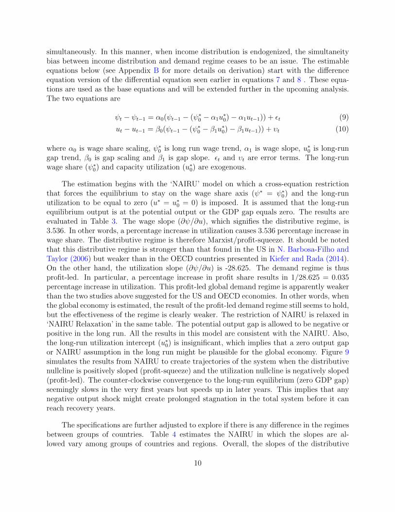
simultaneously. In this manner, when income distribution is endogenized, the simultaneitybias between income distribution and demand regime ceases to be an issue. The estimableequations below (see Appendix B for more details on derivation) start with the differenceequation version of the differential equation seen earlier in equations 7 and 8 . These equa-tions are used as the base equations and will be extended further in the upcoming analysis.The two equations are

ψt − ψt−1 = α0(ψt−1 − (ψ∗0 − α1u

∗0)− α1ut−1)) + εt (9)

ut − ut−1 = β0(ψt−1 − (ψ∗0 − β1u

∗0)− β1ut−1)) + υt (10)

where α0 is wage share scaling, ψ∗0 is long run wage trend, α1 is wage slope, u∗0 is long-run

gap trend, β0 is gap scaling and β1 is gap slope. εt and υt are error terms. The long-runwage share (ψ∗

0) and capacity utilization (u∗0) are exogenous.

The estimation begins with the ‘NAIRU’ model on which a cross-equation restrictionthat forces the equilibrium to stay on the wage share axis (ψ∗ = ψ∗

0) and the long-runutilization to be equal to zero (u∗ = u∗0 = 0) is imposed. It is assumed that the long-runequilibrium output is at the potential output or the GDP gap equals zero. The results areevaluated in Table 3. The wage slope (∂ψ/∂u), which signifies the distributive regime, is3.536. In other words, a percentage increase in utilization causes 3.536 percentage increase inwage share. The distributive regime is therefore Marxist/profit-squeeze. It should be notedthat this distributive regime is stronger than that found in the US in N. Barbosa-Filho andTaylor (2006) but weaker than in the OECD countries presented in Kiefer and Rada (2014).On the other hand, the utilization slope (∂ψ/∂u) is -28.625. The demand regime is thusprofit-led. In particular, a percentage increase in profit share results in 1/28.625 = 0.035percentage increase in utilization. This profit-led global demand regime is apparently weakerthan the two studies above suggested for the US and OECD economies. In other words, whenthe global economy is estimated, the result of the profit-led demand regime still seems to hold,but the effectiveness of the regime is clearly weaker. The restriction of NAIRU is relaxed in‘NAIRU Relaxation’ in the same table. The potential output gap is allowed to be negative orpositive in the long run. All the results in this model are consistent with the NAIRU. Also,the long-run utilization intercept (u∗0) is insignificant, which implies that a zero output gapor NAIRU assumption in the long run might be plausible for the global economy. Figure 9simulates the results from NAIRU to create trajectories of the system when the distributivenullcline is positively sloped (profit-squeeze) and the utilization nullcline is negatively sloped(profit-led). The counter-clockwise convergence to the long-run equilibrium (zero GDP gap)seemingly slows in the very first years but speeds up in later years. This implies that anynegative output shock might create prolonged stagnation in the total system before it canreach recovery years.

The specifications are further adjusted to explore if there is any difference in the regimesbetween groups of countries. Table 4 estimates the NAIRU in which the slopes are al-lowed vary among groups of countries and regions. Overall, the slopes of the distributive

10

and utilization regimes across country groups still strongly indicate profit-led/profit-squeezecharacteristics . Subsequently, Table 5 shows the estimation of NAIRU when the worldeconomy is divided into developed and developing groups of countries. It is interesting tosee that both distributive and demand regimes in developing countries are weaker than indeveloped countries. In developed countries, a percentage increase in capacity utilizationresults in 4.356 percentage increase in wage share, whereas a percentage increase in capacityutilization leads to 3.427 percentage increase in wage share in developing countries. Whilea percentage decrease of wage share can boost a 1/23.739 = 0.042 percentage increase inutilization in developed countries, it only results in a 1/28.314 = 0.035 percentage increasein developing countries.

These results underscore the different characteristics of developed and developing economies.To better illustrate this point, Figure 11 compares the demand regimes and distributiveregimes between two groups. The dotted lines represent developing countries’ distribu-tive/demand regimes while the dashed lines represent developed countries’ two regimes. Asanalyzed above, the developed countries’ distributive curve is steeper, which may indicatethe higher bargaining power of labor unions in advanced countries that are more likely tobe able to pressure for higher wages amidst the economic upturns. The steeper slope ofdeveloping countries’ demand regime in this u − ψ plane automatically translates into theflatter slope of the regime in ψ− u plane. In other words, in the short-run higher utilizationcan be achieved more for developed countries for every percentage reduction in wage share,given other conditions.

Furthermore, the linear trends for both the long-run coordinates are introduced to testif the long run equilibrium might move downwards or upwards. The ψ∗

0 coefficient is reinter-preted as the 1970 wage share equilibrium and u∗0 as the 1970 utilization equilibrium. Thetrends can be negative or positive. The equations can be specified as

ψt − ψt−1 = α0(ψt−1 − (ψ∗0 − α1u

∗0 + (ψ∗

1 − α1u∗1)(date− 1970))− α1ut−1) + εt (11)

ut − ut−1 = β0(ψt−1 − (ψ∗0 − β1u

∗0 + (ψ∗

1 − β1u∗1)(date− 1970))− β1ut−1) + υt (12)

where ψ∗1 is long-run wage share trend and u∗1 is long-run utilization trend. The estimation

results are presented in ‘relaxation with linear trend’ or the last column of Table 3 . Mostcoefficients correspond to the previous results. However, the last two coefficients pose twocrucial points. First, the long-run utilization trend is insignificant. In other words, there isno long-term movement on capacity utilization. Second, the long-run wage trend is negativeand very significant. In other words, there is a long-term downward movement of wageshare. These results implicitly suggest that there is a collective effort to suppress laborincome even though the benefit is not visible in the long run. Further, additional analysis ismade to see if the same results are still valid across groups of countries. The relaxation withlinear trend is separated between developing and developed countries in Table 6 to analyzeif there is any difference in terms of their coefficients and long-term trends. It reveals thatwhile the long-run utilization trends are still insignificant for both groups of countries, the

11

wage trend is significantly worse in developed countries than in developing countries. Thewage trend results are illustrated in Figure 10. The projection exhibits that for more thanfour decades, the gap of long-run wage share between developed and developing countriesirreversibly widens. Even though all the countries have attempted to suppress wages, laborin developed countries suffered more in the last few decades.

Lastly, the structural breaks are investigated since some countries in the sample wereadversely affected by economic crises.7 Two crises, Asian Financial Crisis and Latin Ameri-can Debt Crisis, are scrutinized here. The estimation is interpreted to see if the crisis leadsto any significant shift on wage share or utilization. A dummy coefficient is assigned foryears after or free from the crisis. For the Asian Crisis, the post-era starts at 1998, whereasthe Latin American Debt Crisis starts at 1982 and ends at 2002.8 Table 7 presents theestimation for each crisis covering only the countries in the specific region not the wholesample. For both crises, slopes, intercepts and scaling are not much different from the pre-vious models. However, there are significant negative effects on long-run wage share in bothregions. Asian countries seem to suffer more from the crisis as the negative shift in wageshare is significantly higher. The negative long-run shifts in utilization, on the other hand,is not significant for Asia but significant at 5 percent for Latin America. In other words, thecrisis caused the both negative output and distribution shocks for Latin American countrieswhereas Asian countries suffered only from negative distribution shock after the crisis.

3.3 Discussion: the Global Beggar-My-Neighbor Game

Globalization, financialization and/or technological change have played the main roles indeclining wage share around the world although the extent of each is different for developedand developing countries. Under the neoclassical theory of distribution, income shares aredetermined by technological change. From the 1980s onward, because skill-biased techno-logical improvement has been dominant, new tools, computers and machines have replacedunskilled labor and favored skilled labor by shifting income shares toward them. Technologi-cal progress thus became more capital augmenting than labor augmenting and pushed downwage share. IMF (2007) finds that this has been the main cause of deteriorating wage share

7 The 2008 financial crisis is ignored in this study because many developed countries’ data were ended in2008 in the UN database.

8The Asian Crisis erupted in July 1997 when the Bank of Thailand floated the Thai Baht. The negativeeffect on output had not lasted long and many countries in the region initially recovered within a fewquarters. Nonetheless, the long-term effect on labor, investment and financial sector has been long-lastinguntil today (see Jomo (2007) for more details). However, the story of the Latin American Debt Crisis ismore complicated. The fact that the economic stagnation had prevailed for many years, the so-called ‘LostDecade’, and the crises that recurred in different countries within the region makes it hard to justify thebeginning and the end of the crisis. Here the 1982 Mexican Debt Crisis is identified as the beginning becauseit was the very first crisis involving debt issue in the region and 2002 is marked as the end because it wasthe year Argentina recovered from the economic depression and the commodity boom gradually set off inthe early 2000s (see Ocampo (2014) for more details).

12

in developed countries. However, Stockhammer (2013) finds that globalization, welfare stateretrenchment and financialization significantly contribute to the decline in the wage share,where technological change contributes a very small negative effect in developed countriesand even contributes a positive effect in developing countries.

International trade and finance policies and consequences, therefore, appear to betterexplain why the wage share has fallen over decades. In fact, there has long been a recogni-tion of policies that could capture benefits from globalized markets. In her seminal article,Robinson (1947) argued that an increase in the balance of trade is tantamount to an increasein investment, which usually leads to an increase in employment. As the global market doesnot grow fast enough to accommodate all sales, each nation seeks to increase the share in themarket that will benefit their own people but at the expense of other nations because thebalance of trade of the world as a whole must be zero. This means an increase in exports forone country implies an increase in imports in another. In other words, under internationalcompetition, countries aim to increase their employment by exporting unemployment to therest of the world. A beggar-my-neighbor game is therefore played between nations. Afterone nation succeeds at the expense of others, it will be retaliated against the others. Besidesexport subsidies and import restrictions, the principle devices to increase the balance oftrade are exchange rate depreciation and wage cut. An exchange rate depreciation or a fallin money wages, for instance, would stimulate a primary increase in employment in exportindustries, assuming the Marshal-Lerner condition holds. Put simply, in Robinson’s words,there are four suits in the pack and a country tries to play a higher card out of any suit tobe ahead of others.

The empirical evidence of wage suppression has been ample across the globe, and global-ization appears to result in a negative effect on wage share. Amsden and Hoeven (1996) revealthat many developing countries during the 1980s restructured their manufacturing sectorsby reducing costs, closing inefficient factories and cutting wages to restore profitability. As aresult, the declines in real wages and wage shares were prevalent across countries. Harrison(2005) also confirms the same phenomenon that, based on the panel data of developed anddeveloping countries from 1960 to 2000, rising trade shares and exchange rate crises reducewage share, while an increase in capital intensity, capital controls and government spendingincrease it.Jayadev (2007) instead emphasizes the financial liberalization aspect and foundthat there is a negative relation between capital account openness and labor share. Hisexplanation is that the openness changes the bargaining power of capital against labor asan increase in capital mobility raises rents accruing to capital. Since the early 1980s, anincrease of capital flows has coincided with rising foreign direct investment (FDI) as well.The widening income gap is found to be associated with both FDI outflows from developedcountries and FDI inflows to developing countries. Crotty et al. (1998) explain that whiledeveloped countries might try to delay wage increase in order to slow down job relocation,developing countries may compete with each other for FDI by suppressing wages. The netresult on income tends to be an increase of inequality in both regions. Onaran (2009), inaddition, finds that FDI inflows have a negative effect on wage shares in South Korea, Mexico

13

and Turkey.

The long period collective wage suppression has not translated into higher capital ac-cumulation. On the other side of the same coin, a reduction of wage share is a rise of profitshare. Higher profit share should increase profit expectation on investment for business, sinceprofit acts as an incentive, a source and an outcome of investment (Akyuz and Gore, 1996).After the profit from the initial investment is realized, higher retained earnings encouragefirms to invest more in the next period. Profit is thus a key for investment. However, whenprofit share has risen, often it does not guarantee that it would automatically translate intohigher investment. Profit without production could possibly emerge, especially when firmshave other short-term options to invest or when they need to strengthen their balance sheetsafter the financial crisis erupts (Lapavitsas, 2013) .

Since the 1980s, accumulating evidence shows that the nexus between profit and in-vestment has been weakened both in developed and developing countries (UNCTAD, 2016).By moving decision-making more to shareholder interests relative to other stakeholders, thecommitment of any long-term investment is given less attention even though profit rises.Productive investment is therefore decoupled from profit and replaced with short-term, fi-nancial investment. For business in developed countries, financialization is one of the mainexplanations for the weakening of the profit-investment nexus. The term is defined as theincreasing role of financial motives, financial markets, financial actors and financial institu-tions in the operation of domestic and international economies (Epstein, 2015). Business,as a result, tends to increase its financial activities even among non-financial corporations.The refocusing on financial activities could discourage productive and innovative investment,which could instead create employment. In particular, the pressures from stockholders tomake short-term gains in the stock markets and threats of hostile takeovers when profitdeclines make firms less likely to invest in long-term physical investment projects. There isevidence of the negative relation between financialization in corporate strategy and produc-tive capital formation both in national level (Stockhammer, 2004) and firm-level data (Toriand Onaran, 2015).

The investment slowdown has been observed in developing countries as well. Accordingto Amsden and Hoeven (1996), the consequence of wage suppression during the 1980s was notpleasant for two reasons. First, most non-Asian developing countries suffered a collapse ininvestment. Second, advanced developing countries outside Asia also rolled back their R&Dand technological capability building. After the 1990s, UNCTAD (2016) also finds that onlyAsian developing countries, on average, could maintain their investment shares of GDP. Theinvestment shares, with the exception of Chile, fell moderately in Latin America, while theshares have been volatile in African countries in the past few decades. These different trendsin investment in developing world coupled with the rise of profit shares in many developingcountries underscore the sign of the decoupling of investment-nexus in emerging economiesas well as advanced economies.

14

The long-run consequence of the global race to the bottom and the weakening profit-investment nexus can be illustrated by the Structuralist Goodwin model. Figure 1 showsthe profit-led/profit-squeeze regime in accordance with the results in the previous section.When countries try to gain competitiveness by suppressing wages, it can be interpretedas the anti-labor distributive shock or a rightward shift of the upward sloping distributivecurve. With lower long-run wage share, the profit-led regime should allow the economy tomove toward higher long-run capacity utilization because investment responds positively toa rise in profit share. However, this might not be the case regarding the weakening profit-investment nexus that recently manifested in many countries. Rather, it could imply thatthe negative demand shock may occur and the utilization curve is also shifted to the leftsimultaneously. Investment in this situation does not strongly increase in response to lowerwage share and disallows long-run utilization to increase much, or increase at all. The finalresult could be only a fall in wage share without any gain in capacity utilization in the longrun as suggested in Table 6.

4 Conclusion

Based on the Structuralist Goodwin model, the panel data analysis shows that the worldsystem exhibits a counter-clockwise oscillatory convergence to the equilibrium point in whichwage share is a predator and capacity utilization is a prey. The distributive curve is upward-sloping, which represents a Marxian/profit-squeeze regime. The demand curve is downward-sloping, which implies the regime is profit-led. The results have been confirmed across regionsboth in developed and developing countries. In the short run, developed countries’ demandschedule is more sensitive to a fall in wage share than developing countries’ demand schedule.In the long run, there is no positive gain in utilization while the decline in wage share isintensified, especially in developed countries. The outcome could be interpreted as a resultof the global beggar-my-neighbor game in which nations attempt to reduce wages but cannottranslate into higher investment.

When there is no positive gain in the long-run utilization for the global economy, it mayimply that the divergence between the rich and the poor countries could be perpetuated andglobal inequality would not be alleviated. Since the early 1980s, the conventional idea wasthat after economic integration and market liberalization closed the income gap betweenpoor and rich countries across the world, the income gap between the poor and the richwithin countries would also close too. Most studies, however, have shown that in the pastfew decades, the income gap between rich and poor countries has expanded, in contrast tothe ‘convergence story’ even though markets have been freer and far from strictly regulated(see Pritchett (1997) and Pritchett (2000) among many others). Developed countries haveexperienced more stable growth path while developing countries have been impacted by theperiod of crises and growth collapses. Since 1980, only 20 developing countries have enjoyedperiods of sustained economic growth, or periods of five years or longer during which there

15

was no growth or a decline in income per capita (Ocampo et al., 2007). Milanovic (2016)argues that before the twentieth century, it was ‘class-based inequality,’ inequalities withincountries, that explains the global inequality. Since 1950, surprisingly, seventy percent ofglobal income inequality can be explained by the ‘location-based inequality’ or inequalitiesbetween nations, as a result of growth divergence between the US-Western Europe andthe rest. Together with our results from the empirical analysis, when the long-run gain inutilization is not seen, we may expect that the divergence can further intensify the globalinequality for years to come.

16

References

Akyuz, Yilmaz and Charles Gore (1996). “The Investment-Profits Nexus in East Asian In-dustrialization”. In: World Development 24.3, pp. 461–470. issn: 0305750X. doi: 10.1016/0305-750X(95)00154-5.

Amsden, Alice H and Rolph Van Der Hoeven (1996). “Manufacturing output, employmentand real wages in the 1980s: Labour’s loss until the century’s end”. In: The Journal ofDevelopment Studies 32.4, pp. 506–530.

Atkinson, Anthony B (2015). Inequality. Harvard University Press.Barbosa-Filho, Nelson Henrique (2001). “Essays on Structuralist Macroeconomics”. PhD

thesis. The New School of Social Research.Barbosa-Filho, Nelson and Lance Taylor (2006). “Distributive and Demand Cycles in the

US economy–a structuralist Goodwin model”. In: Metroeconomica 57, pp. 389–411.Bhaduri, Amit and Stephen Marglin (1990). “Unemployment and the Real Wage: the eco-

nomic basis for contesting political ideologies”. In: Cambridge Journal of Economics 14,pp. 375–393.

Blecker, Robert A (1989). “International Competition, Income Distribution and EconomicGrowth”. In: Cambridge Journal of Economics 13, pp. 395–412.

— (2016). “Wage-led versus profit-led demand regimes: the long and short of it”. In: Reviewof Keynesian Economics 4.4, pp. 373–390.

Bowles, Samuel and Robert Boyer (1995). “Wages, Aggregate Demand, and Employmentin an Open Economy: an Empirical Investigation”. In: Macroeconomic Policy after theConservative Era. Cambridge University Press, pp. 143–171.

Carvalho, Laura and Armon Rezai (2015). “Personal Income Inequality and Aggregate De-mand”. In: Cambridge Journal of Economics 40.2, pp. 491–505.

Cogley, T and J M Nason (1995). “Effects of the Hodrick-Prescott filter on trend and dif-ference stationary time series: implications for business cycle reseearch”. In: Journal ofEconomi Dynamics and Control 19, pp. 253–278.

Crotty, James, Gerald Epstein, and Patricia Kelly (1998). “Multinational corporations inthe neo-liberal regime”. In: Globalization and progressive economic policy, pp. 117–143.

Dutt, Amitava K (1984). “Stagnation, income distribution, and monopoly power”. In: Cam-bridge Journal of Economics 8, pp. 25–40.

Ederer, Stefan and Engelbert Stockhammer (2007). “Wages and Aggregate Demand inFrance: an Empirical Investigation”. In: Money, Distribution, and Economic Policy–alternatives to orthodox macroeconomics. Edward Elgar.

Epstein, Gerald (2015). “Financialization: there is something happening here”. In: PoliticalEconomy Research Institute.

Foley, Duncan K and Thomas R Michl (1999). Growth and Distribution. Harvard UniversityPress.

Gollin, Douglas (2002). “Getting Income Shares Right”. In: Journal of Political Economy110.2.

17

Goodwin, Richard M (1967). “A Growth Cycle”. In: Socialism, Capitalism, and Growth.Cambridge University Press.

Hamilton, James D (2017). “Why You Should Never USe the Hodrick-Prescott Filter”. In:NBER Working Paper No. 23429.

Harrison, Ann (2005). “Has Globalization eroded labor’s share? Some cross-country evi-dence”.

Hein, Eckhard and Lena Vogel (2008). “Distribution and Growth Reconsidered: EmpiricalResults for Six OECD Countries”. In: Cambridge Journal of Economics 32, pp. 479–511.

Hirsch, Morris W and Stephen Smale (1974). Differential Equations, Dynamical Systems,and Linear Algebra. New York: Academic Press.

IMF (2007). “The Globalization of Labor”. In: World Economics Outlook. Washington: IMF.Chap. 5.

— (2017). World Economic Outlook. Ed. by IMF.Jayadev, Arjun (2007). “Capital Account Openness and the Labour Share of Income”. In:

Cambridge Journal of Economics 31.3, pp. 423–443.Jomo, K S (2007). “What Did We Really Learn from the 1997-98 Asian Debacle?” In: Ten

Years After: Revisiting the Asian Financial Crisis. Asia Program of the Woodrow WilsonInternational Center for Scholars.

Kaldor, Nicholas (1956). “Alternative Theories of Distribution”. In: Review of EconomicStudies 23, pp. 83–100.

— (1957). “A Model of Economic Growth”. In: The economic Journal 67.268, pp. 591–624.Kalecki, Michal (1971). Selected Essays on the Dynamics of the Capitalist Economy. Cam-

brdige University Press.Karabarbounis, Loukas and Brent Neiman (2013). “The Global Decline of the Labor Share”.

In: The Quarterly Journal of Economics 129.1, pp. 61–103.Keynes, John Maynard (1936). General theory of employment, interest and money. Palgrave

Macmillan.Kiefer, David and Codrina Rada (2014). “Profit Maximising Goes Global: the Race to the

Bottom”. In: Cambridge Journal of Economics 39.5.Lapavitsas, Costas (2013). “The financialization of capitalism: ’Profiting without produc-

ing’”. In: City 17.6, pp. 792–805. issn: 13604813. doi: 10.1080/13604813.2013.853865.Li, Qiang (1999). China’s national income, 1952-1995. Westview Pr.Lotka, A J (1925). Elements of Physical Biology. Williams and Wilkins.Marx, Karl (1867). Capital, volume I. Penguin Classics.Milanovic, Branko (2005). Worlds Apart: Measuring International and Global Inequality.

Princeton University Press.— (2016). Global Inequality: a New Approach for the Age of Globalization. Harvard Univer-

sity Press.Naastepad, C W M and Servaas Storm (2006). “OECD Demand Regimes (1960-2000)”. In:

Journal of Post Keynesian Economics 29.2, pp. 211–246.Nikiforos, Michalis and Duncan K Foley (2012). “Distribution and Capacity Utilization:

Conceptual issues and Empirical Evidence”. In: Metroeconomica 63.1, pp. 200–229.

18

Ocampo, Jose Antonio (2014). “The Latin American Debt Crisis in Historical Perspective”.In: Life after Debt, pp. 87–115.

Ocampo, Jose Antonio, K .S. Jomo, and Rob Vos (2007). “Growth Divergences: ExplainingDifferences in Economic Performance”. In: ed. by Jose Antonio Ocampo, K S Jomo, andRob Vos. United Nations. Chap. Explaining, pp. 1–24.

Onaran, Ozlem (2009). “Wage share, globalization and crisis: the case of the manufacturingindustry in Korea, Mexico and Turkey”. In: International Review of Applied Economics23.2, pp. 113–134.

Onaran, Ozlem and Giorgos Galanis (2012). “Is Aggregate Demand Wage-led or Profit-led?National and Global Effects”. In: ILO Conditions of Work and Employment Series 31.

Piketty, Thomas (2014). Capital in the Twenty-First Century. Harvard University Press.Pritchett, Lant (1997). “Divergence, Big Time”. In: The Journal of Economic Perspectives

11.3, pp. 3–17.— (2000). “Understaning Patterns of Economic Growth: searching for hills among plateaus,

mountains, and plains”. In: The World Bank Economic Review 14.2, pp. 221–250.Qi, Hao (2014). “The Labor Share Question in China”. In: Monthly Review 65.8.Robinson, Joan (1947). “Beggar-my-neighbour remedies for unemployment”. In: Essays on

the theory of employment.Rowthorn, Robert (1981). “Demand, Real Wages and Economic Growth”. In: North East

London Polytechnic.Shone, Ronald (2002). Economic Dynamics: Phase Diagrams and their Economic Applica-

tion. Cambridge University Press.Steindl, Joseph (1952). Maturity and Stagnation in American Capitalism. Basil Blackwell.Stockhammer, Engelbert (2004). “Financialisation and the slowdown of accumulation”. In:

Cambridge Journal of Economics 28.5, pp. 719–741. issn: 0309166X. doi: 10.1093/cje/beh032.

— (2013). “Why Have Wage Shares Fallen? An Analysis of the Determinants of FunctionalIncome Distribution”. In: Wage-led Growth 35, pp. 40–70. doi: 10.1057/9781137357939\_3. url: http://link.springer.com/10.1057/9781137357939_3.

Tavani, Danielle, Peter Flaschel, and Lance Taylor (2011). “Estimated non-linearities andmultiple equilibria in a model of distributive-demand cycles”. In: International Reviewof Applied Economics 25.5, pp. 519–538.

Taylor, Lance (1991). Income Distribution, Inflation, and Growth: Lectures on StructuralistMacroeconomi Theory. MIT Press.

— (2004). Reconstructuring Macroeconomics: Structuralist Proposals and Critiques of theMainstream. Harvard University Press.

Tori, Daniele and Ozlem Onaran (2015). “The effects of financialization on investment: Ev-idence from firm-level data for the UK”. In:

UNCTAD (2012). Trade and Development Report, 2012.— (2016). Trade and Developemtn Report. Tech. rep.

19

Zhou, Xiao M, W Xiao, and X Yao (2010). “Unbalanced Economic Growth and UnevenNational Income Distribution: Evidence from China”. In: Institute for Research on Laborand Employment Working paper.

20

Appendices

A Theoretical Model

Regarding equation (7) and equation (8), a non-trivial stationary solution, where u = 0and ψ = 0, yields the utilization and distributive nullclines of the system, respectively

u = 0→ u = −φ0

φu− φψφuψ (13)

ψ = 0→ ψ = − θ0

θψ− θuθψu (14)

On the u−ψ plane, the slope of demand and distributive curves are important as they signifythe characteristics of each regime. The slopes can be derived as

dψ

du|u=0 = −φu

φψ=βu − αuαψ − βψ

≶ 0 (15)

dψ

du|ψ=0 = − θu

θψ=δu − γuγψ − δψ

≶ 0 (16)

The long-run solution or stable node, where wage share and utilization are constant, can besolved by equating two nullclines or equations (13) and (14) to have

u∗ =θ0φψ − φ0θψφuθψ − θuφψ

ψ∗ =φ0θu − θ0φuφuθψ − θuφψ

(17)

To determine the dynamics and the stability of the system, at the stationary points whereu = ψ = 0, the Jacobian matrix, trace, and determinant can be obtained as

J =

(φu φψθu θψ

)Tr(J) = φu + θψ Det(J) = φuθψ − θuφψ (18)

From this system, the stability condition, as well as the characteristics of each curve, cannotbe determined a priori, since the slopes of both curves, the trace, and the determinant ofthe Jacobian matrix fundamentally depend on how wage share and utilization affect output,potential output, real wage, and labor productivity along the economic cycle. In the nextstep, some economically meaningful closures will be analyzed in order to have phase diagramsof the system. Note that the focus is more on the cases where the nullclines are stable inisolation (φu, θψ < 0) and the system is locally stable (Tr(J) < 0 and Det(J) > o) whichimply that only the signs of φψ and θu are left to be explored.

Considering the demand regime, with Keynesian stability condition, αu is assumedto be negative to decelerate economic growth in the long run as saving is growing faster

21

than investment. Capital accumulation is responded positively to utilization because, byprofit rate accounting, an increase in utilization, given the rates of profit share and organiccomposition of capital, leads to an increase in profit rate. Similarly, a rise of profit share canboost profitability and investment demand. Both arguments thus implicitly mean βu > 0and βψ < 0. From equation (15), we can determine the sign of nominator as positive. Thesign of the slope now depends only upon the sign of αψ or whether the demand schedule iswage-led or profit-led. As the demand regime is determined by whether the size of positiveeffect of increasing wage share on consumption can dominate the negative of increasing wageshare on investment or not, economy is always wage-led (positive slope) when demand iswage-led (αψ > 0). On the other hand, if demand is profit-led (αψ < 0), the overall demandregime is inconclusive. N. Barbosa-Filho and Taylor (2006) finds that in the US the sizeof the negative effect on demand outperforms the negative effect on investment and capitalaccumulation (|αψ| > |βψ|), which forces the slope to be negative, or the profit-led regime.If the opposite case holds, the demand regime is wage-led.

The distributive regime is slightly more complicated when we try to determine the signsof each coefficient. According to Marx’s Reserve Army of Labor hypothesis, economic up-swing will raise labor’s bargaining power as the unemployed is depleted. Real wage thereforetends to vary pro-cyclically (γu > 0). Labor productivity is also assumed to react positivelyto utilization as firms invest more in new technology while they see improving profitability(δu > 0). Now we can see that the sign of the nominator of equation (17) cannot be de-termined a priori. According to N. H. Barbosa-Filho (2001), suppose that growth rate ofreal wage is a negative function of the level of real wage and a positive function of laborproductivity, we thus have a negative relation between wage share and real wage (γψ < 0). Italso suggests that firms invest in labor-saving technology while facing increasing wage share.And since we more emphasize on the the case in which the distributive nullcline is stable inisolation (θψ < 0), this would force δu to be positive. If the δu sign is negative, the sign of γψwill depend on the difference between γψ and δψ. In the prior case, the denominator is forcedto be negative. The sign of the distributive curve will rely only upon the nominator sign. Inparticular, if δu > γu, we will have a forced-saving/Kaldorian distributive regime (negativeslope distributive nullcline). If δu < γu, we will instead have a profit-squeeze/Marxian dis-tributive regime (positive slope distributive nullcline). For stability condition, we disregardthe saddle point case, so the determinant of Jacobian matrix in (18) must only be positive.

B Econometric Model

Given the rate of change is defined as ∆xx

= xt−xt−1

xt−1, the pure or original Goodwin model,

rather than in differential equation form, can be estimated by this following difference-equation specification

22

ψt − ψt−1 = α0ψt−1(ut−1 − u∗) + εt (19)

ut − ut−1 = β0ut−1(ψt−1 − ψ∗) + υt (20)

where ε and υ are error terms. α0 is wage share scaling, β0 is gap scaling and ψ∗0 is long-run

wage intercept. Long-run gap intercept is restricted at zero.

The original version often cannot provide the strong results. Therefore, there must besome adjustments for the equations. The general Goodwin model is an adapted version ofthe original Goodwin model above and can be shown as

ψt − ψt−1 = α0(ψt−1 − (δ1 + δ2ut−1)) + εt (21)

ut − ut−1 = β0(ψt−1 − (δ3 + δ4ut−1)) + υt (22)

At the steady state, ∆ψ and ∆u = 0 , errors are gone, and ψ and u turn to be ψ∗ and u∗,respectively. We have

ψ∗0 = δ1 + δ2u

∗0 (23)

ψ∗0 = δ3 + δ4u

∗0 (24)

Then we solve for δ1 and δ3 to have

δ1 = ψ∗0 − δ2u

∗0 (25)

δ3 = ψ∗0 − δ4u

∗0 (26)

And we plug back δ1 and δ3 into equations (23) and (24) to have

ψt − ψt−1 = α0(ψt−1 − (ψ∗0 − δ2u

∗0)− δ2ut−1)) + εt (27)

ut − ut−1 = β0(ψt−1 − (ψ∗0 − δ4u

∗0)− δ4ut−1)) + υt (28)

where α0 is a wage share scaling, ψ∗0 is the long-run wage trend, α1 is a wage slope, u∗0 is the

long-run gap trend, β0 is a gap scaling and β1 is a gap slope. These equations are used toestimate NAIRU and NAIRU relaxation.

For regional and developed/developing countries differences, the system of equationsbelow simultaneously estimates wage and utilization slopes for each region or group of coun-tries. In particular, the wage and utilization slopes are allowed to vary across different groupof countries. The long-run output gap is set to be zero. The equations are

ψt − ψt−1 = α0(ψt−1 − ψ∗ − δ2ut−1) + εt (29)

ut − ut−1 = β0(ψt−1 − ψ∗ − δ4ut−1) + υt (30)

23

where δ2 and δ4 vary by regions.

Finally, the structural breaks examine the effect from the economic crises. The are twocrises: the Asian Crisis and the Latin American Debt Crisis. The specifications for eachcrisis are tested in separate groups of countries. Since the adverse consequence of each crisiswas limited to the certain countries in the region, not all but only countries affected by thecrisis are tested each time. The system of equation can be transformed into

ψt − ψt−1 = (α0 + β10post)(ψt−1 − (ψ∗0 + ψ∗

10post− (α1 + α11post)(u∗0 + u∗10post))

−(α1 + α11post)ut−1) + εt(31)

ut − ut−1 = (β0 + α10post)(ψt−1 − (ψ∗0 + ψ∗

10post− (β1 + β11post)(u∗0 + u∗10post))

−(β1 + β11post)ut−1) + υt(32)

where post signifies the time period after or free from any crisis.

24

Table 1: Data Summary of Developing Countries

Country Period Average GDP Gap Average Wage Share Index

AfricaAlgeria 1989-2013 -0.375 142.338

Cameroon 1993-2011 -1.074 109.694Kenya 1970-2013 -0.055 98.656

Mauritius 1970-2010 -0.032 115.321Morocco 1998-2013 -0.261 100.025Namibia 1989-2014 -0.097 99.696

South Africa 1970-2014 -0.021 111.887Tunisia 1992-2011 0.114 106.5AsiaChina 1978-2014 0.067 114.38

Hong Kong 1980-2013 0.004 103.139India 1980-2012 -0.17 114.508

Mongolia 1995-2009 -0.919 104.297Philippines 1992-2012 -0.445 92.71Singapore 1980-2012 -0.001 104.437

South Korea 1970-2008 0.35 89.074Sri Lanka 1983-2013 -0.039 89.423Taiwan 1981-2014 0.116 104.87

Thailand 1970-2013 0.087 86.655Latin America

Argentina 1993-2013 0.853 128.222Bolivia 1988-2014 -0.044 99.037Brazil 1992-2009 -0.539 98.707Chile 1974-2013 -0.399 98.711

Colombia 1970-2013 -0.047 107.476Costa Rica 1970-2013 -0.033 94.627

Dominican Republic 1991-2005 -0.455 116.714Honduras 1992-2014 0.059 101.972Jamaica 1998-2014 -0.466 103.342Mexico 1980-2011 0.306 104.756

Nicaragua 1994-2011 0.045 97.696Panama 1989-2012 -0.613 114.086Paraguay 1994-2013 -0.192 110.402

Peru 1970-2011 -0.163 114.826Trinidad and Tobago 1970-2009 -0.097 146.312

Venezuela 1970-2013 0.025 116.92Middle East

Continued on next page

25

Table 1 – continued from previous pageCountry Period Average GDP Gap Average Wage Share IndexBahrain 1992-2014 0.416 116.265

Iran 1994-2011 0.17 105.531Israel 1995-2011 0.366 103.957Oman 1988-2013 -0.38 113.437Turkey 1987-2006 0.25 97.81Europe

Czech Republic 1992-2008 -0.342 99.3Poland 1991-2008 -1.513 110.219

Romania 1989-2008 -1.235 101.387

26

Table 2: Data Summary of Developed Countries

Country Period Average GDP Gap Average Wage Share IndexAustralia 1970-2008 0.037 105.716Austria 1970-2008 0.101 106.183Belgium 1975-2008 0.085 102.587Canada 1970-2006 0.043 106.781

Denmark 1970-2008 0.178 98.472Finland 1970-2008 0.199 104.596France 1970-2009 0.049 101.658

Germany 1970-2008 0.094 105.245Iceland 1973-2005 -0.395 83.777Ireland 1970-2008 0.263 115.061Italy 1970-2008 0.15 107.75

Japan 1970-2011 -0.035 100.422Luxembourg 1970-2008 0.172 102.782Netherlands 1970-2008 0.097 104.895

Norway 1970-2009 0.086 116.03Portugal 1977-2010 0.179 88.959

Spain 1980-2008 0.135 98.63Sweden 1970-2008 0.15 105.785

UK 1970-2005 -0.044 101.155US 1970-2011 -0.002 105.732

27

Figure 1: A profit-led/profit-squeeze Structuralist Goodwin Model with stable wage share dy-namics (upward-sloping Distributive Nullcline and downward-sloping Utilization Nullcline)

28

Figure 2: A wage-led/wage-squeeze Structuralist Goodwin Model with stable wage share dy-namics (downward-sloping Distributive Nullcline and upward-sloping Utilization Nullcline)

29

Figure 3: A profit-led/wage-squeeze Structuralist Goodwin Model with unstable wage sharedynamics (downward-sloping Distributive Nullcline and downward-sloping Utilization Null-cline

30

Figure 4: Original and Adjusted Wage Share of Brazil (absolute numbers)

31

Figure 5: Decreasing Wage Share Trends in Developed Countries

Figure 6: Increasing Wage Share Trends in Developed Countries

32

Figure 7: Decreasing Wage Share Trends in Developing Countries

Figure 8: Increasing Wage Share Trends in Developing Countries

33

Figure 9: Trajectories from NAIRU

34

Figure 10: Long run linear Trend estimates of state variables

35

Figure 11: Comparison of NAIRU Developed vs Developing Countries’ Regimes

36

Table 3: Econometric Results (t-statistics in the parentheses)

Coefficients NAIRUNAIRU

RelaxationRelaxation with

linear trendWage Slope (α1) 3.536 3.626 3.547

(35.296) (32.894) (33.339)Utilization Slope (β1) -28.625 -30.053 -29.365

(-14.521) (-13.187) (-13.286)Wage Share Scaling (α0) -0.095 -0.093 -0.095

(-44.078) (-42.109) (-42.844)Utilization Scaling (β0) -0.013 -0.012 -0.012

(-14.831) (-13.239) (-13.286)Long Run Wage Intercept (ψ∗

0) 103.419 103.646 107.828(511.3) (397.704) (205.519)

Long run Utilization intercept (u∗0) 0.044 0.027(0.91) (0.248)

Long run Wage trend (ψ∗1) -0.169

(-8.76)Long run Utilization trend (u∗1) 0.0008

(0.21)Schwarz Criterion 2221.427 2197.185 2296.467

Table 4: Econometric Results by Regions (t-statistics in the parentheses)

RegionWage Share

SlopeUtilization

SlopeType Dynamics

Africa 4.63 -32.322 Profit-Squeeze/Profit-led Stable(14.905) (-14.656)

Asia 3.324 -29.067 Profit-Squeeze/Profit-led Stable(21.804) (-14.146)

Europe 1.648 -21.921 Profit-Squeeze/Profit-led Stable(4.06) (-12.283)

Latin America 3.45 -26.464 Profit-Squeeze/Profit-led Stable(19.423) (-14.027)

Middle East 3.884 -34.172 Profit-Squeeze/Profit-led Stable(7.42) (-12.074)

Developed Countries 4.372 -23.27 Profit-Squeeze/Profit-led Stable(34.559) (-14.042)

Schwarz Criterion 2121.447

37

Table 5: Econometric Results of Developed/Developing Countries (t-statistics in the paren-theses)

Coefficients NAIRUDeveloping Countries Developed Countries

Wage Slope (α1) 3.427 4.356(28.1) (34.872)

Utilization Slope (β1) -28.314 -23.739(-14.976) (-13.947)

Wage Share Scaling (α0) -0.094(-43.921)

Utilization Scaling (β0) -0.013(-15.182)

Long Run Wage Intercept (ψ∗0) 103.512

(494.821)Schwarz Criterion 2135.219

Table 6: Econometric Results of Developed/Developing Countries with Linear Trends (t-statistics in the parentheses)

Coefficients Relaxation with Linear TrendDeveloping Countries Developed Countries

Wage Slope (α1) 3.314 4.277(27.731) (33.211)

Utilization Slope (β1) -29.625 -28.49(-12.904) (-12.521)

Wage Share Scaling (α0) -0.097(-44.368)

Utilization Scaling (β0) -0.012(-12.972)

Long Run Wage Intercept (ψ∗0) 108.588

(210.9997)Long run Utilization intercept (u∗0) -0.081

(-0.786)Long run Wage trend (ψ∗

1) -0.147 -0.303(-7.6) (-13.186)

Long run Utilization trend (u∗1) 0.004 0.005(0.965) (1.199)

Schwarz Criterion 2275.98

38

Table 7: Econometric Results of Structural Breaks (t-statistics in the parentheses)

Coefficients Asian CrisisLatin American

Debt CrisisWage Slope (α1) 6.604 5.827

(2.587) (2.115)Utilization Slope (β1) 97.276 -11.437

(0.368) (-2.534)Wage Share Scaling (α0) -0.03 -0.055

(-3.075) (-2.227)Utilization Scaling (β0) 0.003 -0.025

(0.369) (-2.739)Long run Wage Intercept (ψ∗

0) 117.253 110.619(13.633) (25.962)

Long run Utilization Intercept (u∗0) 0.949 0.686(1.068) (1.591)

Shift in wage slope (α11) -4.64 -3.44(-1.799) (-1.225)

Shift in Utilization slope (β11) -110.871 -23.65(-0.419) (-1.224)

Shift in Wage Share Scaling (α10) -0.038 0.013(-2.492) (1.176)

Shift in Utilization Scaling (β10) -0.181 -0.063(-6.201) (-2.069)

Shift in Long run Wage (ψ∗10) -15.763 -9.662

(-1.827) (-2.126)Shift in Long run Utilization (u∗10) -1.311 -1.135

(-1.376) (-2.092)Schawarz Criterion 1870.598 3469.666

39