A Global Climatology of Explosive Cyclones using aMulti-Tracking Approach
Marco Reale, Margarida L.R. Liberato, Piero Lionello, Joaquim G. Pinto,Stefano Salon & Sven Ulbrich
To cite this article: Marco Reale, Margarida L.R. Liberato, Piero Lionello, Joaquim G. Pinto,Stefano Salon & Sven Ulbrich (2019) A Global Climatology of Explosive Cyclones using aMulti-Tracking Approach, Tellus A: Dynamic Meteorology and Oceanography, 71:1, 1-19, DOI:10.1080/16000870.2019.1611340
To link to this article: https://doi.org/10.1080/16000870.2019.1611340
A Global Climatology of Explosive Cyclones using aMulti-Tracking Approach
By MARCO REALE1,2�, MARGARIDA L.R. LIBERATO3,4, PIERO LIONELLO5,6, JOAQUIM G.PINTO7, STEFANO SALON2, and SVEN ULBRICH8,9, 1Abdus Salam ICTP, strada costiera 11,
Trieste, Italy; 2Istituto di Oceanografia e di Geofisica Sperimentale - OGS, Via Beirut 2-4, Trieste;3Universidade de Tr�as-os-Montes e Alto Douro, UTAD, Vila Real, Portugal; 4Instituto Dom Luiz
(IDL), Faculdade de Ciencias, Universidade de Lisboa, Lisboa, Portugal; 5DiSTeBA, Universit�a delSalento, Lecce, Italy; 6CMCC, Lecce, Italy; 7Institute of Meteorology and Climate Research, KarlsruheInstitute of Technology, Karlsruhe, Germany; 8Institute for Geophysics and Meteorology, University of
Cologne, Germany; 9Department FE12–Data Assimilation, Deutscher Wetterdienst, Germany
(Manuscript received 4 October 2018; in final form 17 January 2017)
ABSTRACTIn this study, hemispheric climatologies of explosive cyclones (ECs) derived using a set of different cyclonedetection and tracking methods (CDTMs) are analysed. The aim is to evaluate trends and regionalcharacteristics of ECs discussing consensus and disagreement among methods. Areas of both hemispherescharacterised by relatively frequent presence of ECs are considered, with particular emphasis on theirextremes. Despite the considerable differences (up to 21-38% in the Northern/Southern Hemisphere) in thetotal number of ECs detected by the various CDTM, this study provides evidence of a good level ofagreement among methods concerning spatial distribution of cyclogenesis, track density, their maincharacteristics (depth, speed, duration, deepening and normalised deepening rate), seasonality and trends.ECs are shown to be deeper, faster and long-lasting with respect to ordinary cyclones in both hemispheres.Southern Hemisphere ECs are typically more intense than those in Northern Hemisphere. On the other hand,ECs in the Northern Hemisphere are characterised by a stronger deepening rate over 6 h and 24h than in theSouthern Hemisphere. Atlantic ECs are usually faster, deeper and characterised by higher deepening andgeostrophically adjusted deepening rate than in the Pacific. This is particularly true in the eastern part of thebasin. In both basins, ECs in the western side are characterised by higher normalised deepening rates than inthe eastern parts. In the Southern Hemisphere, ECs close to Southern Africa and Australia are usually faster,deeper and with higher deepening rates than those close to southern South America. On the other hand, ECsclose to southern South America and Southern Africa are characterised by higher normalised deepening ratesand duration with respect to ECs close to Australia.
Cyclones are a key component in the mid-latitude atmos-phere dynamics. They play a fundamental role in thehydrological cycle, in the meridional transport of energy,moisture and momentum (e.g. Peixoto and Oort, 1992).Cyclones are strongly linked with meteorological hazards,such as strong winds, marine storms, storm surges,intense precipitation, floods and landslides and, thus,with economic losses and fatalities (e.g. De Zolt et al.,
2006; Nissen et al., 2010; Liberato et al., 2011; 2013;Pinto et al., 2013; Reale and Lionello, 2013;Liberato, 2014).
Explosive cyclones (or so-called meteorological“bombs”, hereafter ECs) are characterised with respectto “ordinary” cyclones (or non-explosive cyclones, here-after NECs) by a strong deepening rate (depending onlatitude) in a relative short time range. Historically, ECsare identified through a “Normalised Central PressureDeepening Rate” (NDRc, Sanders and Gyakum, 1980)defined as:�Corresponding author. e-mail: [email protected]
Tellus A: 2019. # 2019 The Author(s). Published by Informa UK Limited, trading as Taylor & Francis Group.This is an Open Access article distributed under the terms of the Creative Commons Attribution-NonCommercial License (http://creativecommons.org/licenses/by-nc/4.0/), which permits unrestricted non-commercial use, distribution, and reproduction in any medium, provided the original work is properlycited.
where DR24h is the variation of central pressure over aperiod of 24 h, u is the latitude of cyclone and 60� is theso-called “reference latitude”. When NDRc exceeds theunity, the system is deemed to be an EC (Sanders andGyakum, 1980). In the Southern Hemisphere this defin-ition has been challenged as it may lead to the identifica-tion of many artificial/spurious systems (Lim andSimmonds, 2002; Allen et al., 2010). In fact, according to(1) a system moving meridionally towards a lower pres-sure area experiences a strong deepening due to the vari-ation of pressure field background that does notcorrespond to a real increase in the strength of the systemitself. Therefore, it has been suggested to use either a“Normalised Reference Pressure Deepening Rate”(NDRr) so that DR24h corresponds to the anomaly withrespect to the climatology field, or to use an approachcombining NDRr/NDRc metrics together (Lim andSimmonds, 2002; Allen et al., 2010).
ECs form in both hemispheres mainly during the coldseason in regions with enhanced baroclinicity associatedto strong horizontal temperature gradients (e.g. to theeast of continental coastlines), large moisture availabilityand enhanced jet stream velocities (Roebber, 1984;Sanders, 1986; Gyakum et al., 1989; Chen et al., 1992;Stull, 2000; Chang et al., 2002; Allen et al., 2010; Seilerand Zwiers, 2016). Due to the rapid decrease of the cen-tral pressure, these systems are associated with extremestrong circulation and thus with extreme events like windgusts, heavy rain potentially leading to floods, andextreme height waves (Sanders and Gyakum, 1980; Finket al., 2009; Liberato et al., 2011).
Over the last 40 years, studies on ECs have beenfocused on deriving a climatology in Northern/SouthernHemisphere (hereafter NH/SH; e.g. Roebber, 1984; Limand Simmonds, 2002; Allen et al., 2010; Seiler andZwiers, 2016) or in specific regions (Sanders, 1986; Chenet al., 1992; Wang and Rogers, 2001; Trigo, 2006;Kuwano-Yoshida and Asuma, 2008; Kouroutzoglouet al., 2011), on associated physical processes and telecon-nections (e.g. Fink et al., 2012; G�omara et al., 2014) oron specific case studies (e.g. Liberato et al., 2011; Ludwiget al., 2014). For example, Allen et al. (2010) have shownthat ECs are distributed into several distinct regions,including two regions of maximum density in the NHcorresponding to the Northwest Pacific and NorthAtlantic and three regions in the Southern Hemisphere incorrespondence to East of Southern America, between45E–90E, poleward of 40S and in an area correspondingto 100E–150W/45S-80S. Seiler and Zwiers (2016) haveevaluated the ability of CMIP5 to reproduce ECs andshown that most of the models reproduce well their
spatial distribution in comparison with the reanalyses inthe NH, with two maxima along the Kuroshio and theGulf Stream. Furthermore, Liberato et al. (2011) haveanalysed the case of the storm Klaus, which affectedEurope (mainly France and Spain) on 23–24 January2009 and was associated with heavy rain, snow over thePyrenees, record breaking wind gusts (up to 55ms�1),high waves over the Bay of Biscay and WesternMediterranean (up to 15m) and considerable societalimpacts including fatalities. All these studies have appliedcyclone detection and tracking methods (hereafterCTDMs; Neu et al., 2013; Lionello et al., 2016) to reanal-yses or climate models data.
While the above-described climatological studies arevalid assessments of the ECs activity in both hemispheres,they can be influenced by the choice and resolution ofthe reanalyses/GCMs used and by the choice of CDTMitself (Allen et al., 2010). For example, depending on howa cyclone is defined, a CDTM may use for the detectionand tracking different atmospheric variables, such asmean sea level pressure (MSLP) or relative vorticity (Neuet al., 2013), leading to the identification of different pos-ition centres and intensification rates for the same storm.
The IMILAST (Intercomparison of MId LAtitudeSTorm Diagnostics, Neu et al., 2013; Ulbrich et al., 2013;Hewson and Neu, 2015; Rudeva et al., 2014; Lionelloet al., 2016; Pinto et al., 2016; Grieger et al., 2018) pro-ject has provided evidence of the potentiality of a multiCDTM approach for identifying and describing the entirelife cycle of cyclones. Neu et al. (2013) have shown thatall CDTMs approaches applied to ERA-interim datasetproduce comparable climatologies of cyclones in the NH/SH, with a general high agreement among differentCDTMs for deep cyclones and for the frequency, lifecycle, inter-annual variability and trends of these systems.Based on selected case studies, Neu et al. (2013) showedthat the level of agreement among CDTMs in describingthe cyclone life cycle is high during the intense phase ofthe storm, low during its previous development and lysis.On the other hand, Ulbrich et al. (2013) have shown thatdespite different numbers of cyclones identified applyingdifferent CDTMs to ECHAM5/OM1 model simulation,the climate change signal is similar among all theCDTMs. Hewson and Neu (2015) have analysed thestructure and characteristics of windstorms affectingNorthern Atlantic and Europe identifying three causalclasses of these systems. Rudeva et al. (2014) have ana-lysed the sensitivity of cyclone climatology to the filteringover orography exceeding 1500m, time of detection andrepresentation of fast moving cyclones, providing evi-dence that filtering and late identification of cyclonesreduces significantly the number of cyclones, while thesplitting of trajectories has negligible effect on cyclone
2 M. REALE ET AL.
distribution as well as on the average deepening rate.Lionello et al. (2016) have discussed the consensus amongdifferent CDTMs on the climatology of cyclones in theMediterranean region, with a spread among methodsmainly due to how each CDTM deals with slow andweak cyclones. Pinto et al. (2016) have shown that multiCDTMs approach qualitatively identifies cyclone clustersaffecting the Euro-Atlantic Region inDecember–January–February and, in particular, thatunder dispersion and over dispersion of extratropicalcyclones over the North Atlantic and Western Europe arefeatures generally robust with respect to the choice ofCDTM. Finally Grieger et al. (2018) analysed extratrop-ical cyclone activity around the Antarctica showing that,despite a different number of tracks identified by eachCDTM, the multi CDTMs pointed out the existence ofrobust trends in the area for these systems and that thelevel of agreement is high among the methods when thecomparison is limited to stronger systems. All the previ-ous works, thus, have pointed out that one of importantsource of spreading among different CDTMs rely on howthese different approaches deal with slow/fast and weak/deep cyclones and a multi CDTMs approach can provide,indeed, a more robust description of cyclone activity inboth hemispheres.
In the present manuscript, we focus on the characteris-tics of ECs from the multi-methodology CDTMs perspec-tive. The main purposes of this work are as follows:� to extract separated datasets of ECs and NECs for
both hemispheres based on the original IMILASTdataset of cyclone tracks (Neu et al., 2013)
� to derive a comprehensive climatology of ECs inboth hemispheres and assess their main characteris-tics with respect to NECs
� to use this climatology to compare characteristics ofECs among target regions in both hemispheres withparticular emphasis on extremes, intensity andtrends, assessing the statistical significance of the dif-ferences observed.
The work is organised as follows. Section 2 provides adescription of the procedure for the identification of ECs,the features of the new ECs/NECs datasets and the statis-tical tools used in this work. Section 3 analyses the cli-matology of ECs in both NH/SH with a comparison oftheir features with respect to NECs and among them-selves in different areas of both hemispheres. Finally,Section 4 includes the discussions of the results, conclu-sions and future developments of the work.
2. Data and methods
In this study, we consider ECs originated polewardsbeyond the 25� parallel in both hemispheres. The analysis
of ECs activity and the relatively comparison with NECsis based on eight different CDTM (Table 1) applied tothe Mean Sea Level Pressure (MSLP) fields of the 6-hourly ERA-Interim 1979–2008 at 1.5� resolution. For afull description of each CDTM, the reader is referred toNeu et al. (2013) and references in Table 1. Each CDTMprovides a list of cyclones with a lifetime longer than24 h, their position as a function of time and differentvariables describing their intensity (like MSLP,Laplacian, Geopotential Height, Neu et al., 2013). TheseCDTMs differ among them in employing different met-rics for the detection and tracking of cyclones (such asminimum MSLP, Relative Vorticity, intensity of wind,maximum of Laplacian of SLP, maximum gradient ofSLP) or different thresholds for removing/merging artifi-cial/weak systems (Neu et al., 2013). Among the list ofmethods that contributed to the IMILAST dataset (Neuet al., 2013), we have chosen the eight tracking methods(Table 1) based on MSLP.
Cyclones for each of the methods have been then div-ided in ECs and NECs and two separate datasets havebeen built covering the period January 1979–December2008. The variables used to describe both classes of cyclo-nes are: position (in longitude and latitude), SLP value ofthe central minimum (hPa), deepening rate (DR6h, hPa/6h), geostrophically adjusted deepening rate (ADR6h,hPa/6h), normalised central deepening rate (equation 1,NDRc in hPa/24h), adjusted normalised central deepeningrate (ADNDRc, in hPa/24h), speed (in km/h), distancecovered in 6 h (in km) and two flags (0 or 1) to markwhen the cyclone becomes EC and reaches its maximumADR6h. These variables are defined as follows:� DR6h: the variation of pressure in a cyclone in two
consecutive timesteps� ADR6h (Trigo, 2006): (DR6h)�sin(60�)/sin(u) where
u is the latitude of cyclone and 60� is the so-calledreference latitude
� ADNDRc: (DR24h/24h)�sin(60�)/sin(uav) where uav isthe latitude of the mean position of cyclone in 24hand 60� is again the reference latitude
Table 1. List of cyclone detection and tracking methods used inthis study with code number in the IMILAST dataset and mainbibliographic reference for the description of each method.
Method References
M02 Murray and Simmonds, 1991; Pinto et al., 2005M06 Hewson, 1997; Hewson and Titley, 2010M08 Trigo, 2006M09 Serreze, 1995; Wang et al., 2006M10 Murray and Simmonds, 1991; Simmonds et al., 2008M16 Lionello et al., 2002; Reale and Lionello, 2013M20 Wernli and Schwierz, 2006M22 Bardin and Polonsky, 2005; Akperov et al., 2007
THEMATIC CLUSTER: INTERCOMPARISON OF MID-LATITUDE STORM DIAGNOSTICS 3
In the computation of NDRc and ADNDRc, followingthe IMILAST protocol (Neu et al., 2013), we considered24 h as a period of five consecutive time steps.
ECs are defined as all the systems which fulfil the crite-ria of equation (1) based on the NDRc (Sanders andGyakum, 1980) while the category NECs includes all thesystems which does not fulfil the criteria based on equa-tion (1) and has a maximum ADR6h/NDRc lower thanzero (this in order to filter away systems identified byeach CDTM with no negative observed deepening ratesalong their life cycle). Recently, the criterion of equation(1) has been criticised and other criteria have been sug-gested (Allen et al., 2010). However we have kept the ori-ginal formulation, as the main purpose of this work isnot to compare the sensitivity of the climatology of ECswith respect to different detection criteria, but to derive ageneral climatology using a multi tracking approach.
Following the multi tracking approach introduced inprevious works (Neu et al., 2013; Ulbrich et al., 2013;Hewson and Neu, 2015; Rudeva et al., 2014; Flaounaset al., 2016; Lionello et al., 2016; Pinto et al., 2016) weexplore the consensus in term of trends for the ECs com-puting a multi-method mean (MCDTM, Neu et al., 2013;Lionello et al, 2016). To show a possible common behav-iour among the time series in both hemispheres a normal-ised index ECindex has been computed for each i-method,defined as
where EC(i,t) is the number of ECs in the i-method atthe time t, ECaverage(i) the average of the timeseries,stdEC(i) is its standard deviation. The Mann–Kendalltest (MK) has been adopted for assessing the significanceof trends in the historical time series. Additional statis-tical tools are considered and described in the regionalanalysis (Section 3.3).
Finally, boxplots are used to compare ECs and NECsin order to determine the most frequent minimum valueof SLP (hereafter MSLPmin, meant for the whole duration
of the cyclone) and the most frequent maximum value ofDR6h, ADR6h, NDRc, speed (hereafter DRmax, ADRmax,NDRcmax, speedmax) and duration at hemispheric scale.Particular emphasis has been given to extremes in someselected areas of both Hemispheres.
3. Results
3.1. ECs climatologies
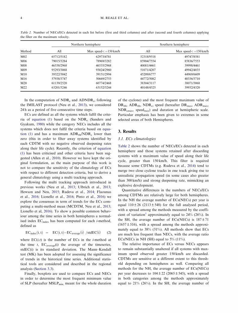
Table 2 shows the number of NECs/ECs detected in eachhemisphere and those systems retained after discardingsystems with a maximum value of speed along their lifecycle, greater than 150 km/h. This filter is requiredbecause some CDTMs (e.g. Rudeva et al., 2014) tend tomerge two close cyclone tracks in one track giving rise tounrealistic propagation speed (in some cases also greaterthan 300 km/h) and strong deepening rate, mimicking anexplosive development.
Quantitative differences in the numbers of NECs/ECsamong CDTMs are relatively large for both hemispheres.In the NH the average number of ECs(NECs) per year isequal 110± 26 (2113± 548) for the full analysed period,with a spread among the methods measured by the coeffi-cient of variation1 approximately equal to 24% (26%). Inthe SH, the average number of ECs(NECs) is 187± 71(1657± 516), with a spread among the methods approxi-mately equal to 38% (31%). All methods show that ECsare much less frequent than NECs, with the average ratioECs/NECs in NH (SH) equal to 5% (11%).
The relative importance of ECs versus NECs appearsto remain substantially unaltered if all systems with max-imum speed observed greater 150 km/h are discarded.CDTMs are sensitive at a different extent to this thresh-old depending on hemispheres as well. Comparing allmethods for the NH, the average number of ECs(NECs)per year decreases to 104± 22 (2065± 545), with a spreadin both categories among the methods approximatelyequal to 21% (26%). In the SH, the average number of
Table 2. Number of NECs/ECs detected in each list before (first and third columns) and after (second and fourth columns) applyingthe filter on the maximum velocity.
ECs (NEC) decreases to 176± 67 (1620± 524) with aspread among the methods approximately equal to 38%(32%). It appears that the uncertainties raising from veryfast propagating cyclones affect mainly ECs in the NHand it is probably linked to the larger area with orog-raphy higher than 1500m in the NH, where this error hasbeen observed (Rudeva et al., 2014). For the rest of thepaper the analysis will include only ECs and NECs withmaximum propagation speed lower than 150 km/h. Thenumber of ECs detected in NH (SH) tends to be higher(is in good agreement) with respect to Allen et al. (2010)(80 ECs in the NH and 171 ECs per year in SH) andhigher with respect to Lim, and Simmonds (2002) (26.4ECs in the SH and 45.9 in the NH). However, these num-bers are not directly comparable with our results as inAllen et al. (2010) a single CDTM was employed while in
Lim and Simmonds (2002) the detection of ECs has beencarried out using NDRr approach instead of our clas-sical approach.
3.2. Temporal and spatial variability of ECs
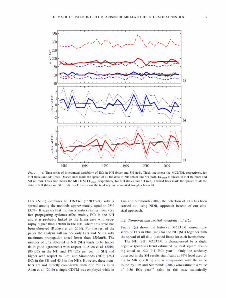
Figure 1(a) shows the historical MCDTM annual timeseries of ECs in blue (red) for the NH (SH) together withthe spread of all data (dashed lines) for each hemisphere.
The NH (SH) MCDTM is characterised by a slightnegative (positive) trend estimated by least square result-ing equal to –0.2 (0.4) ECs year�1. Only the tendencyobserved in the SH results significant at 95% level accord-ing to MK (p< 0.05) and is comparable with the valuefound by Lim and Simmonds (2002) who estimate a valueof 0.56 ECs year�1 (also in this case statistically
Fig. 1. (a) Time series of interannual variability of ECs in NH (blue) and SH (red). Thick line shows the MCDTM, respectively, forNH (blue) and SH (red). Dashed lines mark the spread of all the data in NH (blue) and SH (red). ECindex is shown in NH (b, blue) andSH (c, red). Thick line shows the MCDTM ECindex, respectively, for NH (blue) and SH (red). Dashed lines mark the spread of all thedata in NH (blue) and SH (red). Black lines show the tendency line computed trough a linear fit.
THEMATIC CLUSTER: INTERCOMPARISON OF MID-LATITUDE STORM DIAGNOSTICS 5
significant). The positive tendencies observed in the NHby Lim and Simmonds (2002) and Allen et al. (2010)were not statistically significant. Figure 1(b,c) shows thetime series of the corresponding ECindex described inequation (2) for both hemispheres. The spread among themethods dramatically reduces and again the MCDTMshows in NH (SH) a slight negative (positive) linear trendequal to –0.02 (0.03).
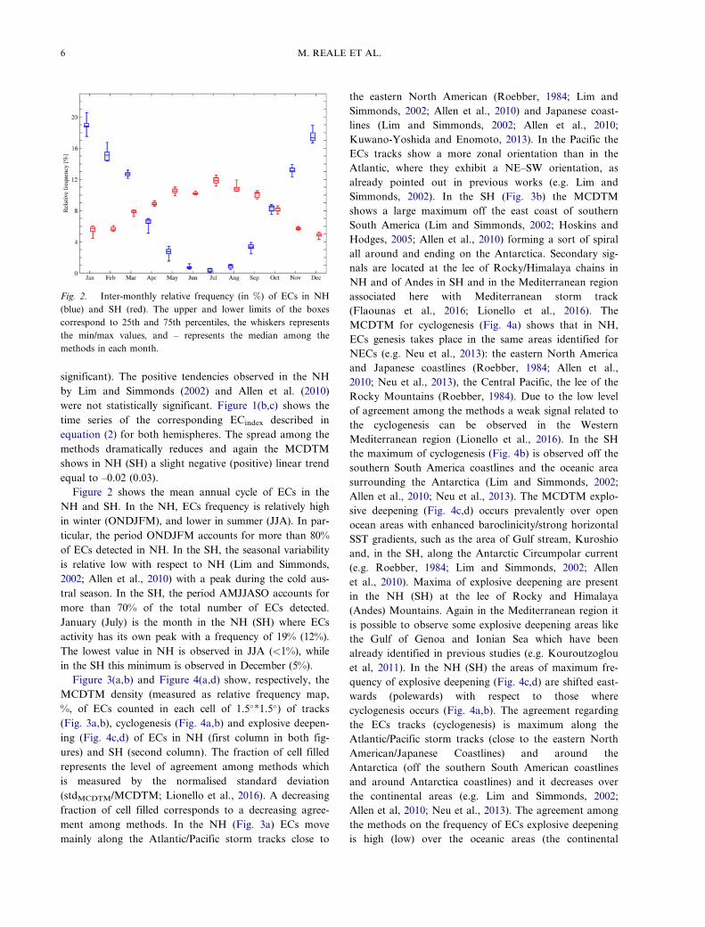
Figure 2 shows the mean annual cycle of ECs in theNH and SH. In the NH, ECs frequency is relatively highin winter (ONDJFM), and lower in summer (JJA). In par-ticular, the period ONDJFM accounts for more than 80%of ECs detected in NH. In the SH, the seasonal variabilityis relative low with respect to NH (Lim and Simmonds,2002; Allen et al., 2010) with a peak during the cold aus-tral season. In the SH, the period AMJJASO accounts formore than 70% of the total number of ECs detected.January (July) is the month in the NH (SH) where ECsactivity has its own peak with a frequency of 19% (12%).The lowest value in NH is observed in JJA (<1%), whilein the SH this minimum is observed in December (5%).
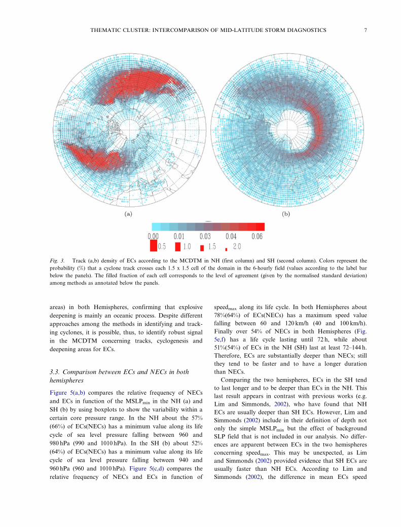
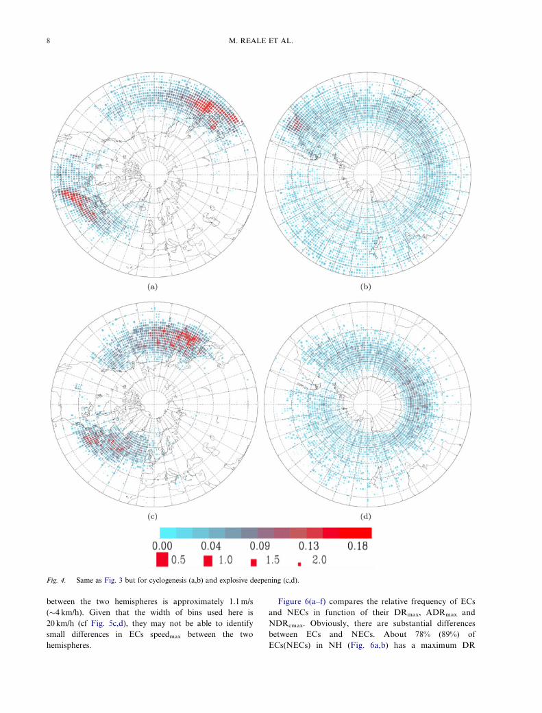
Figure 3(a,b) and Figure 4(a,d) show, respectively, theMCDTM density (measured as relative frequency map,%, of ECs counted in each cell of 1.5��1.5�) of tracks(Fig. 3a,b), cyclogenesis (Fig. 4a,b) and explosive deepen-ing (Fig. 4c,d) of ECs in NH (first column in both fig-ures) and SH (second column). The fraction of cell filledrepresents the level of agreement among methods whichis measured by the normalised standard deviation(stdMCDTM/MCDTM; Lionello et al., 2016). A decreasingfraction of cell filled corresponds to a decreasing agree-ment among methods. In the NH (Fig. 3a) ECs movemainly along the Atlantic/Pacific storm tracks close to
the eastern North American (Roebber, 1984; Lim andSimmonds, 2002; Allen et al., 2010) and Japanese coast-lines (Lim and Simmonds, 2002; Allen et al., 2010;Kuwano-Yoshida and Enomoto, 2013). In the Pacific theECs tracks show a more zonal orientation than in theAtlantic, where they exhibit a NE–SW orientation, asalready pointed out in previous works (e.g. Lim andSimmonds, 2002). In the SH (Fig. 3b) the MCDTMshows a large maximum off the east coast of southernSouth America (Lim and Simmonds, 2002; Hoskins andHodges, 2005; Allen et al., 2010) forming a sort of spiralall around and ending on the Antarctica. Secondary sig-nals are located at the lee of Rocky/Himalaya chains inNH and of Andes in SH and in the Mediterranean regionassociated here with Mediterranean storm track(Flaounas et al., 2016; Lionello et al., 2016). TheMCDTM for cyclogenesis (Fig. 4a) shows that in NH,ECs genesis takes place in the same areas identified forNECs (e.g. Neu et al., 2013): the eastern North Americaand Japanese coastlines (Roebber, 1984; Allen et al.,2010; Neu et al., 2013), the Central Pacific, the lee of theRocky Mountains (Roebber, 1984). Due to the low levelof agreement among the methods a weak signal related tothe cyclogenesis can be observed in the WesternMediterranean region (Lionello et al., 2016). In the SHthe maximum of cyclogenesis (Fig. 4b) is observed off thesouthern South America coastlines and the oceanic areasurrounding the Antarctica (Lim and Simmonds, 2002;Allen et al., 2010; Neu et al., 2013). The MCDTM explo-sive deepening (Fig. 4c,d) occurs prevalently over openocean areas with enhanced baroclinicity/strong horizontalSST gradients, such as the area of Gulf stream, Kuroshioand, in the SH, along the Antarctic Circumpolar current(e.g. Roebber, 1984; Lim and Simmonds, 2002; Allenet al., 2010). Maxima of explosive deepening are presentin the NH (SH) at the lee of Rocky and Himalaya(Andes) Mountains. Again in the Mediterranean region itis possible to observe some explosive deepening areas likethe Gulf of Genoa and Ionian Sea which have beenalready identified in previous studies (e.g. Kouroutzoglouet al, 2011). In the NH (SH) the areas of maximum fre-quency of explosive deepening (Fig. 4c,d) are shifted east-wards (polewards) with respect to those wherecyclogenesis occurs (Fig. 4a,b). The agreement regardingthe ECs tracks (cyclogenesis) is maximum along theAtlantic/Pacific storm tracks (close to the eastern NorthAmerican/Japanese Coastlines) and around theAntarctica (off the southern South American coastlinesand around Antarctica coastlines) and it decreases overthe continental areas (e.g. Lim and Simmonds, 2002;Allen et al, 2010; Neu et al., 2013). The agreement amongthe methods on the frequency of ECs explosive deepeningis high (low) over the oceanic areas (the continental
Fig. 2. Inter-monthly relative frequency (in %) of ECs in NH(blue) and SH (red). The upper and lower limits of the boxescorrespond to 25th and 75th percentiles, the whiskers representsthe min/max values, and – represents the median among themethods in each month.
6 M. REALE ET AL.
areas) in both Hemispheres, confirming that explosivedeepening is mainly an oceanic process. Despite differentapproaches among the methods in identifying and track-ing cyclones, it is possible, thus, to identify robust signalin the MCDTM concerning tracks, cyclogenesis anddeepening areas for ECs.
3.3. Comparison between ECs and NECs in bothhemispheres
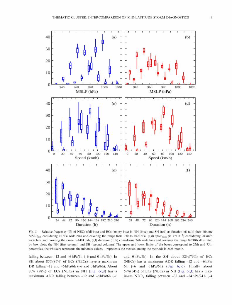
Figure 5(a,b) compares the relative frequency of NECsand ECs in function of the MSLPmin in the NH (a) andSH (b) by using boxplots to show the variability within acertain core pressure range. In the NH about the 57%(66%) of ECs(NECs) has a minimum value along its lifecycle of sea level pressure falling between 960 and980 hPa (990 and 1010 hPa). In the SH (b) about 52%(64%) of ECs(NECs) has a minimum value along its lifecycle of sea level pressure falling between 940 and960 hPa (960 and 1010 hPa). Figure 5(c,d) compares therelative frequency of NECs and ECs in function of
speedmax along its life cycle. In both Hemispheres about78%(64%) of ECs(NECs) has a maximum speed valuefalling between 60 and 120 km/h (40 and 100 km/h).Finally over 54% of NECs in both Hemispheres (Fig.5e,f) has a life cycle lasting until 72 h, while about51%(54%) of ECs in the NH (SH) last at least 72–144 h.Therefore, ECs are substantially deeper than NECs; stillthey tend to be faster and to have a longer durationthan NECs.
Comparing the two hemispheres, ECs in the SH tendto last longer and to be deeper than ECs in the NH. Thislast result appears in contrast with previous works (e.g.Lim and Simmonds, 2002), who have found that NHECs are usually deeper than SH ECs. However, Lim andSimmonds (2002) include in their definition of depth notonly the simple MSLPmin but the effect of backgroundSLP field that is not included in our analysis. No differ-ences are apparent between ECs in the two hemispheresconcerning speedmax. This may be unexpected, as Limand Simmonds (2002) provided evidence that SH ECs areusually faster than NH ECs. According to Lim andSimmonds (2002), the difference in mean ECs speed
Fig. 3. Track (a,b) density of ECs according to the MCDTM in NH (first column) and SH (second column). Colors represent theprobability (%) that a cyclone track crosses each 1.5 x 1.5 cell of the domain in the 6-hourly field (values according to the label barbelow the panels). The filled fraction of each cell corresponds to the level of agreement (given by the normalised standard deviation)among methods as annotated below the panels.
THEMATIC CLUSTER: INTERCOMPARISON OF MID-LATITUDE STORM DIAGNOSTICS 7
between the two hemispheres is approximately 1.1m/s(�4 km/h). Given that the width of bins used here is20 km/h (cf Fig. 5c,d), they may not be able to identifysmall differences in ECs speedmax between the twohemispheres.
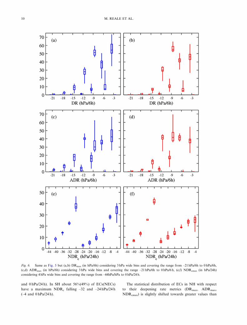
Figure 6(a–f) compares the relative frequency of ECsand NECs in function of their DRmax, ADRmax andNDRcmax. Obviously, there are substantial differencesbetween ECs and NECs. About 78% (89%) ofECs(NECs) in NH (Fig. 6a,b) has a maximum DR
Fig. 4. Same as Fig. 3 but for cyclogenesis (a,b) and explosive deepening (c,d).
8 M. REALE ET AL.
falling between –12 and –6 hPa/6h (–6 and 0 hPa/6h). InSH about 85%(86%) of ECs (NECs) have a maximumDR falling –12 and –6 hPa/6h (–6 and 0 hPa/6h). About70% (78%) of ECs (NECs) in NH (Fig. 6c,d) has amaximum ADR falling between –12 and –6 hPa/6h (–6
and 0 hPa/6h). In the SH about 82%(79%) of ECs(NECs) has a maximum ADR falling –12 and –6 hPa/6h (–6 and 0 hPa/6h) (Fig. 6c,d). Finally about59%(64%) of ECs (NECs) in NH (Fig. 6e,f) has a max-imum NDRc falling between –32 and –24 hPa/24 h (–4
Fig. 5. Relative frequency (%) of NECs (full box) and ECs (empty box) in NH (blue) and SH (red) as function of: (a,b) their lifetimeMSLPmin considering 10hPa wide bins and covering the range from 930 to 1020hPa, (c,d) speedmax (in km h�1) considering 20km/hwide bins and covering the range 0–140 km/h, (e,f) duration (in h) considering 24h wide bins and covering the range 0–240 h illustratedby box plots: the NH (first column) and SH (second column). The upper and lower limits of the boxes correspond to 25th and 75thpercentiles, the whiskers represents the min/max values, – represents the median among the methods in each month.
THEMATIC CLUSTER: INTERCOMPARISON OF MID-LATITUDE STORM DIAGNOSTICS 9
and 0 hPa/24 h). In SH about 56%(49%) of ECs(NECs)have a maximum NDRc falling –32 and –24 hPa/24 h(–4 and 0 hPa/24 h).
The statistical distribution of ECs in NH with respectto their deepening rate metrics (DRmax, ADRmax,NDRcmax) is slightly shifted towards greater values than
Fig. 6. Same as Fig. 5 but (a,b) DRmax (in hPa/6h) considering 3 hPa wide bins and covering the range from –21hPa/6h to 0 hPa/6h,(c,d) ADRmax (in hPa/6h) considering 3 hPa wide bins and covering the range –21hPa/6h to 0 hPa/6 h, (e,f) NDRcmax (in hPa/24h)considering 4 hPa wide bins and covering the range from –44hPa/hPa to 0 hPa/24 h.
10 M. REALE ET AL.
in SH, suggesting in general larger deepening rates. Thisis in agreement with previous studies (Lim andSimmonds, 2002; Allen et al., 2010), which have shownthat extreme values of NDRc are more frequent in theNH, as it is characterised by pronounced baroclinic envir-onment with respect to the SH.
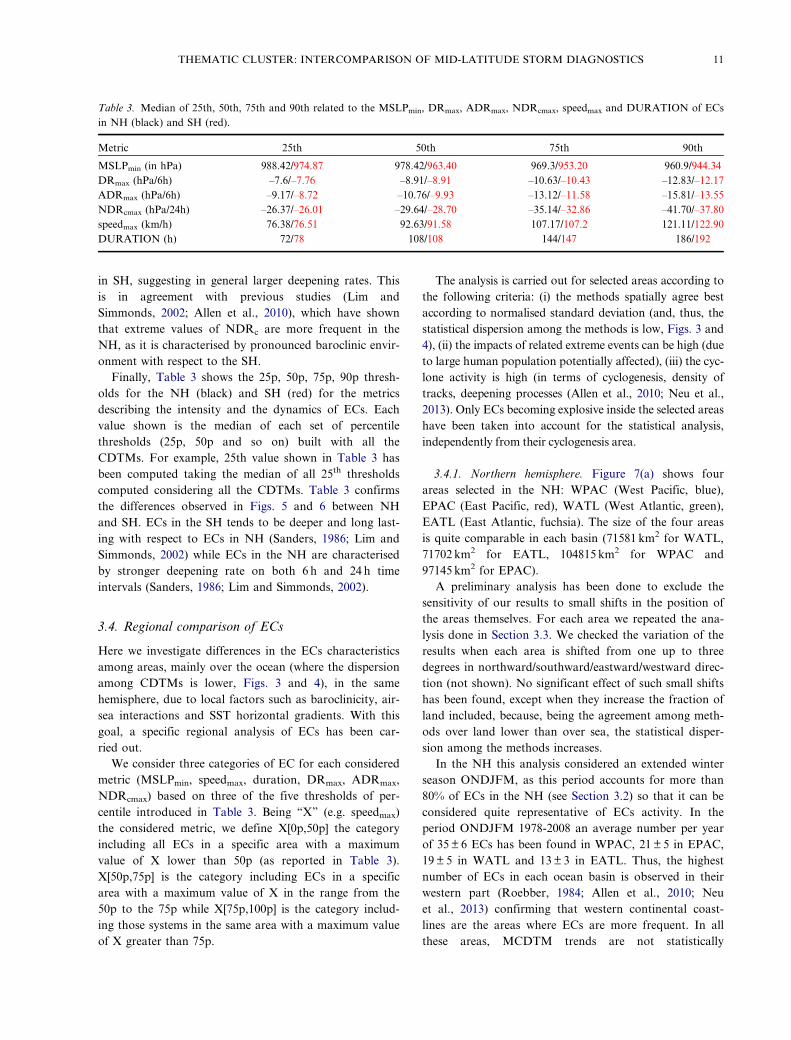
Finally, Table 3 shows the 25p, 50p, 75p, 90p thresh-olds for the NH (black) and SH (red) for the metricsdescribing the intensity and the dynamics of ECs. Eachvalue shown is the median of each set of percentilethresholds (25p, 50p and so on) built with all theCDTMs. For example, 25th value shown in Table 3 hasbeen computed taking the median of all 25th thresholdscomputed considering all the CDTMs. Table 3 confirmsthe differences observed in Figs. 5 and 6 between NHand SH. ECs in the SH tends to be deeper and long last-ing with respect to ECs in NH (Sanders, 1986; Lim andSimmonds, 2002) while ECs in the NH are characterisedby stronger deepening rate on both 6 h and 24 h timeintervals (Sanders, 1986; Lim and Simmonds, 2002).
3.4. Regional comparison of ECs
Here we investigate differences in the ECs characteristicsamong areas, mainly over the ocean (where the dispersionamong CDTMs is lower, Figs. 3 and 4), in the samehemisphere, due to local factors such as baroclinicity, air-sea interactions and SST horizontal gradients. With thisgoal, a specific regional analysis of ECs has been car-ried out.
We consider three categories of EC for each consideredmetric (MSLPmin, speedmax, duration, DRmax, ADRmax,NDRcmax) based on three of the five thresholds of per-centile introduced in Table 3. Being “X” (e.g. speedmax)the considered metric, we define X[0p,50p] the categoryincluding all ECs in a specific area with a maximumvalue of X lower than 50p (as reported in Table 3).X[50p,75p] is the category including ECs in a specificarea with a maximum value of X in the range from the50p to the 75p while X[75p,100p] is the category includ-ing those systems in the same area with a maximum valueof X greater than 75p.
The analysis is carried out for selected areas according tothe following criteria: (i) the methods spatially agree bestaccording to normalised standard deviation (and, thus, thestatistical dispersion among the methods is low, Figs. 3 and4), (ii) the impacts of related extreme events can be high (dueto large human population potentially affected), (iii) the cyc-lone activity is high (in terms of cyclogenesis, density oftracks, deepening processes (Allen et al., 2010; Neu et al.,2013). Only ECs becoming explosive inside the selected areashave been taken into account for the statistical analysis,independently from their cyclogenesis area.
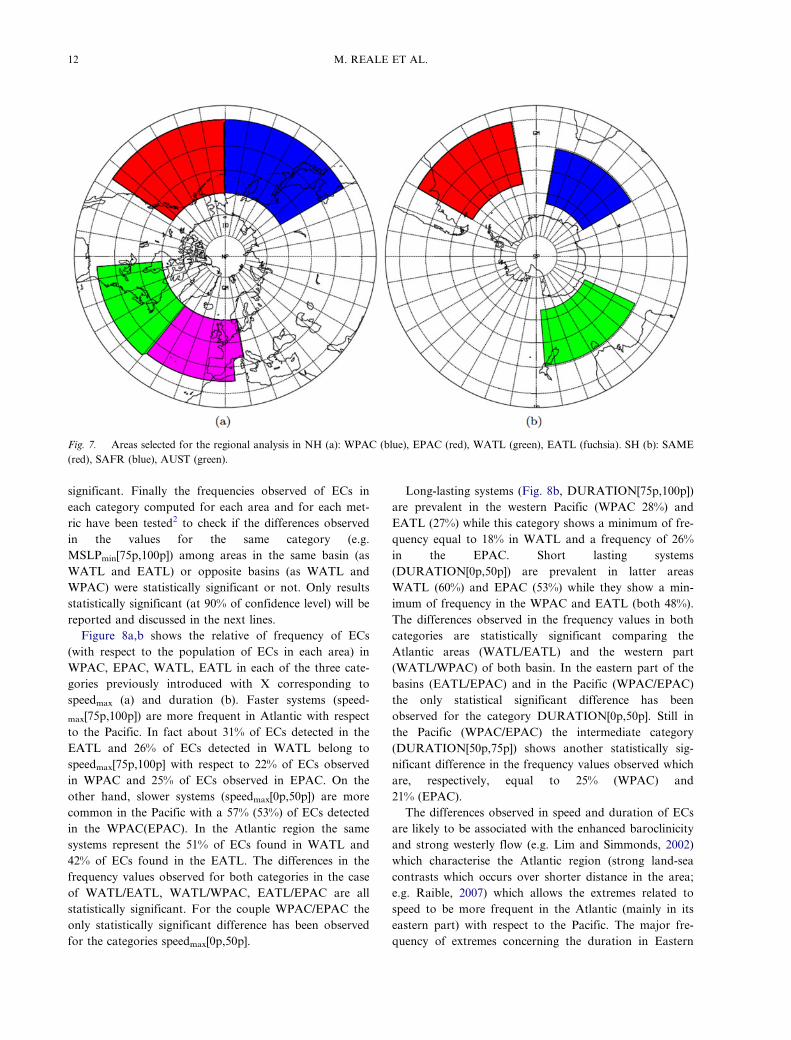
3.4.1. Northern hemisphere. Figure 7(a) shows fourareas selected in the NH: WPAC (West Pacific, blue),EPAC (East Pacific, red), WATL (West Atlantic, green),EATL (East Atlantic, fuchsia). The size of the four areasis quite comparable in each basin (71581 km2 for WATL,71702 km2 for EATL, 104815 km2 for WPAC and97145 km2 for EPAC).
A preliminary analysis has been done to exclude thesensitivity of our results to small shifts in the position ofthe areas themselves. For each area we repeated the ana-lysis done in Section 3.3. We checked the variation of theresults when each area is shifted from one up to threedegrees in northward/southward/eastward/westward direc-tion (not shown). No significant effect of such small shiftshas been found, except when they increase the fraction ofland included, because, being the agreement among meth-ods over land lower than over sea, the statistical disper-sion among the methods increases.
In the NH this analysis considered an extended winterseason ONDJFM, as this period accounts for more than80% of ECs in the NH (see Section 3.2) so that it can beconsidered quite representative of ECs activity. In theperiod ONDJFM 1978-2008 an average number per yearof 35± 6 ECs has been found in WPAC, 21± 5 in EPAC,19± 5 in WATL and 13± 3 in EATL. Thus, the highestnumber of ECs in each ocean basin is observed in theirwestern part (Roebber, 1984; Allen et al., 2010; Neuet al., 2013) confirming that western continental coast-lines are the areas where ECs are more frequent. In allthese areas, MCDTM trends are not statistically
Table 3. Median of 25th, 50th, 75th and 90th related to the MSLPmin, DRmax, ADRmax, NDRcmax, speedmax and DURATION of ECsin NH (black) and SH (red).
THEMATIC CLUSTER: INTERCOMPARISON OF MID-LATITUDE STORM DIAGNOSTICS 11
significant. Finally the frequencies observed of ECs ineach category computed for each area and for each met-ric have been tested2 to check if the differences observedin the values for the same category (e.g.MSLPmin[75p,100p]) among areas in the same basin (asWATL and EATL) or opposite basins (as WATL andWPAC) were statistically significant or not. Only resultsstatistically significant (at 90% of confidence level) will bereported and discussed in the next lines.
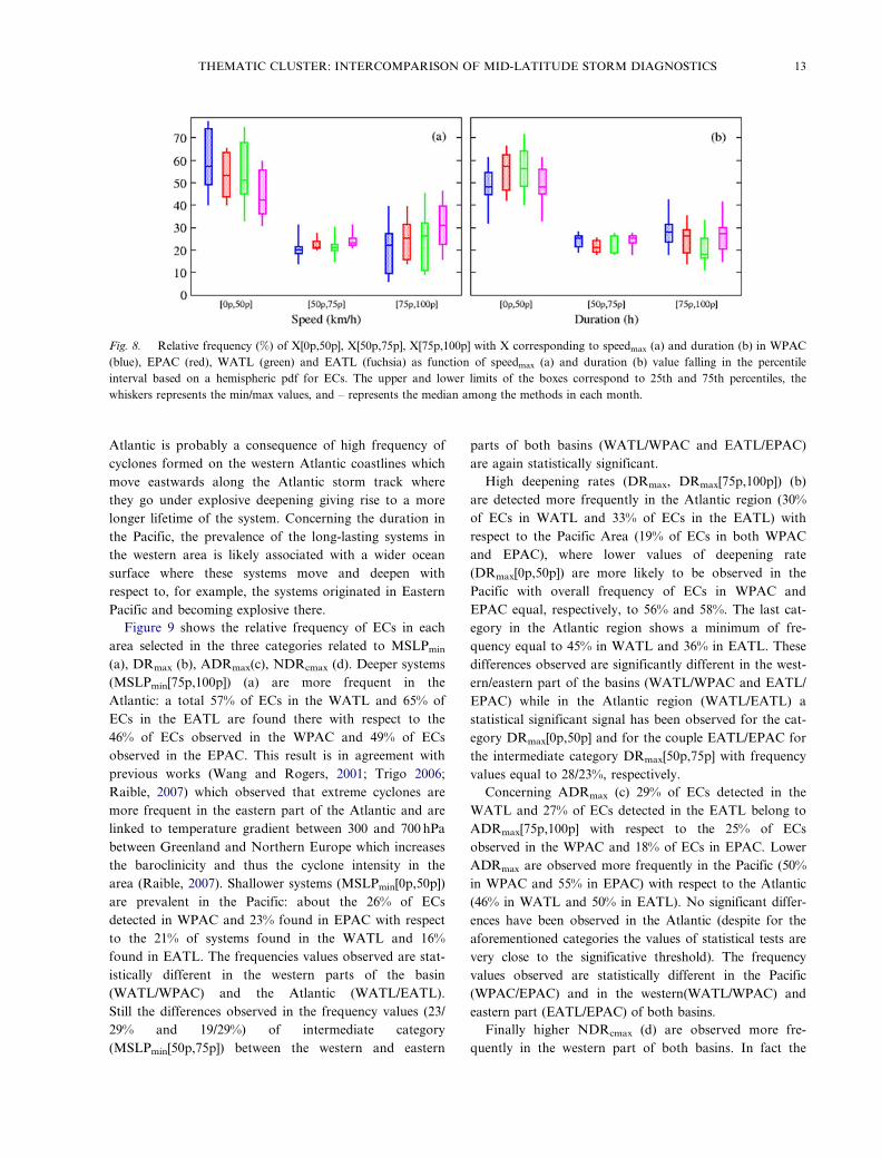
Figure 8a,b shows the relative of frequency of ECs(with respect to the population of ECs in each area) inWPAC, EPAC, WATL, EATL in each of the three cate-gories previously introduced with X corresponding tospeedmax (a) and duration (b). Faster systems (speed-
max[75p,100p]) are more frequent in Atlantic with respectto the Pacific. In fact about 31% of ECs detected in theEATL and 26% of ECs detected in WATL belong tospeedmax[75p,100p] with respect to 22% of ECs observedin WPAC and 25% of ECs observed in EPAC. On theother hand, slower systems (speedmax[0p,50p]) are morecommon in the Pacific with a 57% (53%) of ECs detectedin the WPAC(EPAC). In the Atlantic region the samesystems represent the 51% of ECs found in WATL and42% of ECs found in the EATL. The differences in thefrequency values observed for both categories in the caseof WATL/EATL, WATL/WPAC, EATL/EPAC are allstatistically significant. For the couple WPAC/EPAC theonly statistically significant difference has been observedfor the categories speedmax[0p,50p].
Long-lasting systems (Fig. 8b, DURATION[75p,100p])are prevalent in the western Pacific (WPAC 28%) andEATL (27%) while this category shows a minimum of fre-quency equal to 18% in WATL and a frequency of 26%in the EPAC. Short lasting systems(DURATION[0p,50p]) are prevalent in latter areasWATL (60%) and EPAC (53%) while they show a min-imum of frequency in the WPAC and EATL (both 48%).The differences observed in the frequency values in bothcategories are statistically significant comparing theAtlantic areas (WATL/EATL) and the western part(WATL/WPAC) of both basin. In the eastern part of thebasins (EATL/EPAC) and in the Pacific (WPAC/EPAC)the only statistical significant difference has beenobserved for the category DURATION[0p,50p]. Still inthe Pacific (WPAC/EPAC) the intermediate category(DURATION[50p,75p]) shows another statistically sig-nificant difference in the frequency values observed whichare, respectively, equal to 25% (WPAC) and21% (EPAC).
The differences observed in speed and duration of ECsare likely to be associated with the enhanced baroclinicityand strong westerly flow (e.g. Lim and Simmonds, 2002)which characterise the Atlantic region (strong land-seacontrasts which occurs over shorter distance in the area;e.g. Raible, 2007) which allows the extremes related tospeed to be more frequent in the Atlantic (mainly in itseastern part) with respect to the Pacific. The major fre-quency of extremes concerning the duration in Eastern
Fig. 7. Areas selected for the regional analysis in NH (a): WPAC (blue), EPAC (red), WATL (green), EATL (fuchsia). SH (b): SAME(red), SAFR (blue), AUST (green).
12 M. REALE ET AL.
Atlantic is probably a consequence of high frequency ofcyclones formed on the western Atlantic coastlines whichmove eastwards along the Atlantic storm track wherethey go under explosive deepening giving rise to a morelonger lifetime of the system. Concerning the duration inthe Pacific, the prevalence of the long-lasting systems inthe western area is likely associated with a wider oceansurface where these systems move and deepen withrespect to, for example, the systems originated in EasternPacific and becoming explosive there.
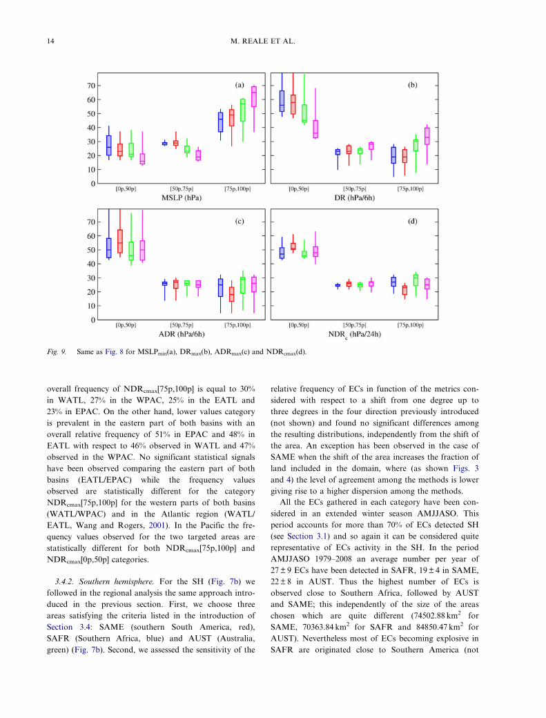
Figure 9 shows the relative frequency of ECs in eacharea selected in the three categories related to MSLPmin
(a), DRmax (b), ADRmax(c), NDRcmax (d). Deeper systems(MSLPmin[75p,100p]) (a) are more frequent in theAtlantic: a total 57% of ECs in the WATL and 65% ofECs in the EATL are found there with respect to the46% of ECs observed in the WPAC and 49% of ECsobserved in the EPAC. This result is in agreement withprevious works (Wang and Rogers, 2001; Trigo 2006;Raible, 2007) which observed that extreme cyclones aremore frequent in the eastern part of the Atlantic and arelinked to temperature gradient between 300 and 700 hPabetween Greenland and Northern Europe which increasesthe baroclinicity and thus the cyclone intensity in thearea (Raible, 2007). Shallower systems (MSLPmin[0p,50p])are prevalent in the Pacific: about the 26% of ECsdetected in WPAC and 23% found in EPAC with respectto the 21% of systems found in the WATL and 16%found in EATL. The frequencies values observed are stat-istically different in the western parts of the basin(WATL/WPAC) and the Atlantic (WATL/EATL).Still the differences observed in the frequency values (23/29% and 19/29%) of intermediate category(MSLPmin[50p,75p]) between the western and eastern
parts of both basins (WATL/WPAC and EATL/EPAC)are again statistically significant.
High deepening rates (DRmax, DRmax[75p,100p]) (b)are detected more frequently in the Atlantic region (30%of ECs in WATL and 33% of ECs in the EATL) withrespect to the Pacific Area (19% of ECs in both WPACand EPAC), where lower values of deepening rate(DRmax[0p,50p]) are more likely to be observed in thePacific with overall frequency of ECs in WPAC andEPAC equal, respectively, to 56% and 58%. The last cat-egory in the Atlantic region shows a minimum of fre-quency equal to 45% in WATL and 36% in EATL. Thesedifferences observed are significantly different in the west-ern/eastern part of the basins (WATL/WPAC and EATL/EPAC) while in the Atlantic region (WATL/EATL) astatistical significant signal has been observed for the cat-egory DRmax[0p,50p] and for the couple EATL/EPAC forthe intermediate category DRmax[50p,75p] with frequencyvalues equal to 28/23%, respectively.
Concerning ADRmax (c) 29% of ECs detected in theWATL and 27% of ECs detected in the EATL belong toADRmax[75p,100p] with respect to the 25% of ECsobserved in the WPAC and 18% of ECs in EPAC. LowerADRmax are observed more frequently in the Pacific (50%in WPAC and 55% in EPAC) with respect to the Atlantic(46% in WATL and 50% in EATL). No significant differ-ences have been observed in the Atlantic (despite for theaforementioned categories the values of statistical tests arevery close to the significative threshold). The frequencyvalues observed are statistically different in the Pacific(WPAC/EPAC) and in the western(WATL/WPAC) andeastern part (EATL/EPAC) of both basins.
Finally higher NDRcmax (d) are observed more fre-quently in the western part of both basins. In fact the
Fig. 8. Relative frequency (%) of X[0p,50p], X[50p,75p], X[75p,100p] with X corresponding to speedmax (a) and duration (b) in WPAC(blue), EPAC (red), WATL (green) and EATL (fuchsia) as function of speedmax (a) and duration (b) value falling in the percentileinterval based on a hemispheric pdf for ECs. The upper and lower limits of the boxes correspond to 25th and 75th percentiles, thewhiskers represents the min/max values, and – represents the median among the methods in each month.
THEMATIC CLUSTER: INTERCOMPARISON OF MID-LATITUDE STORM DIAGNOSTICS 13
overall frequency of NDRcmax[75p,100p] is equal to 30%in WATL, 27% in the WPAC, 25% in the EATL and23% in EPAC. On the other hand, lower values categoryis prevalent in the eastern part of both basins with anoverall relative frequency of 51% in EPAC and 48% inEATL with respect to 46% observed in WATL and 47%observed in the WPAC. No significant statistical signalshave been observed comparing the eastern part of bothbasins (EATL/EPAC) while the frequency valuesobserved are statistically different for the categoryNDRcmax[75p,100p] for the western parts of both basins(WATL/WPAC) and in the Atlantic region (WATL/EATL, Wang and Rogers, 2001). In the Pacific the fre-quency values observed for the two targeted areas arestatistically different for both NDRcmax[75p,100p] andNDRcmax[0p,50p] categories.
3.4.2. Southern hemisphere. For the SH (Fig. 7b) wefollowed in the regional analysis the same approach intro-duced in the previous section. First, we choose threeareas satisfying the criteria listed in the introduction ofSection 3.4: SAME (southern South America, red),SAFR (Southern Africa, blue) and AUST (Australia,green) (Fig. 7b). Second, we assessed the sensitivity of the
relative frequency of ECs in function of the metrics con-sidered with respect to a shift from one degree up tothree degrees in the four direction previously introduced(not shown) and found no significant differences amongthe resulting distributions, independently from the shift ofthe area. An exception has been observed in the case ofSAME when the shift of the area increases the fraction ofland included in the domain, where (as shown Figs. 3and 4) the level of agreement among the methods is lowergiving rise to a higher dispersion among the methods.
All the ECs gathered in each category have been con-sidered in an extended winter season AMJJASO. Thisperiod accounts for more than 70% of ECs detected SH(see Section 3.1) and so again it can be considered quiterepresentative of ECs activity in the SH. In the periodAMJJASO 1979–2008 an average number per year of27± 9 ECs have been detected in SAFR, 19± 4 in SAME,22± 8 in AUST. Thus the highest number of ECs isobserved close to Southern Africa, followed by AUSTand SAME; this independently of the size of the areaschosen which are quite different (74502.88 km2 forSAME, 70363.84 km2 for SAFR and 84850.47 km2 forAUST). Nevertheless most of ECs becoming explosive inSAFR are originated close to Southern America (not
Fig. 9. Same as Fig. 8 for MSLPmin(a), DRmax(b), ADRmax(c) and NDRcmax(d).
14 M. REALE ET AL.
shown) confirming that western Southern American con-tinental coastlines are the areas where cyclogenesis proc-esses are more frequent in the SH (e.g. Lim andSimmonds, 2002; Allen et al.,2010; Neu et al., 2013). Nosignificant tendencies have been observed in MCDTM inthese areas according to MK.
Figure 10(a,b) shows the relative frequency of ECs inSAME, SAFR and AUST gathering according to speedmax
(a) and duration (b). Faster systems (speedmax[75p,100p])are more frequent in SAFR (28% of ECs detected here)and in AUST (26.5%). SAME shows lower frequency val-ues (22%) for this category and a maximum frequencyvalue of 51.5% for speedmax[0p,50p] with respect to 50.5%and 46.5% observed, respectively, observed in AUST andSAFR. The frequency values of both categories areresulted to be statistically different comparing SAME/SAFR and for the category speedmax[75p,100p] in the caseof the couple SAME/AUST. Long-lasting system ECs(DURATION[75p,100p])) are prevalent in SAME (27.5%of EC detected) and in SAFR (26.5%) with respect to the23.5% of ECs observed in AUST where short lasting sys-tems (DURATION[0p,50p]) are prevalent (56%). The onlystatistical significant difference for the frequency valueshave been observed comparing both categories in the caseof the couple SAFR/AUST and for the couple SAME/AUST in the case of the category DURATION[0p,50p].
So while in the case of SAME/SAFR ECs tend to lastmore probably because once they formed, they travelgreater distance due to interaction with the ocean belowfollowing the spiral path observed in Fig. 3(b) in the caseof speedmax the higher baroclinicity of SAFR and AUSTassociated with Circumpolar current and the positionwith respect to the Antarctica (Lim and Simmonds, 2002)result in faster ECs with respect to SAME.
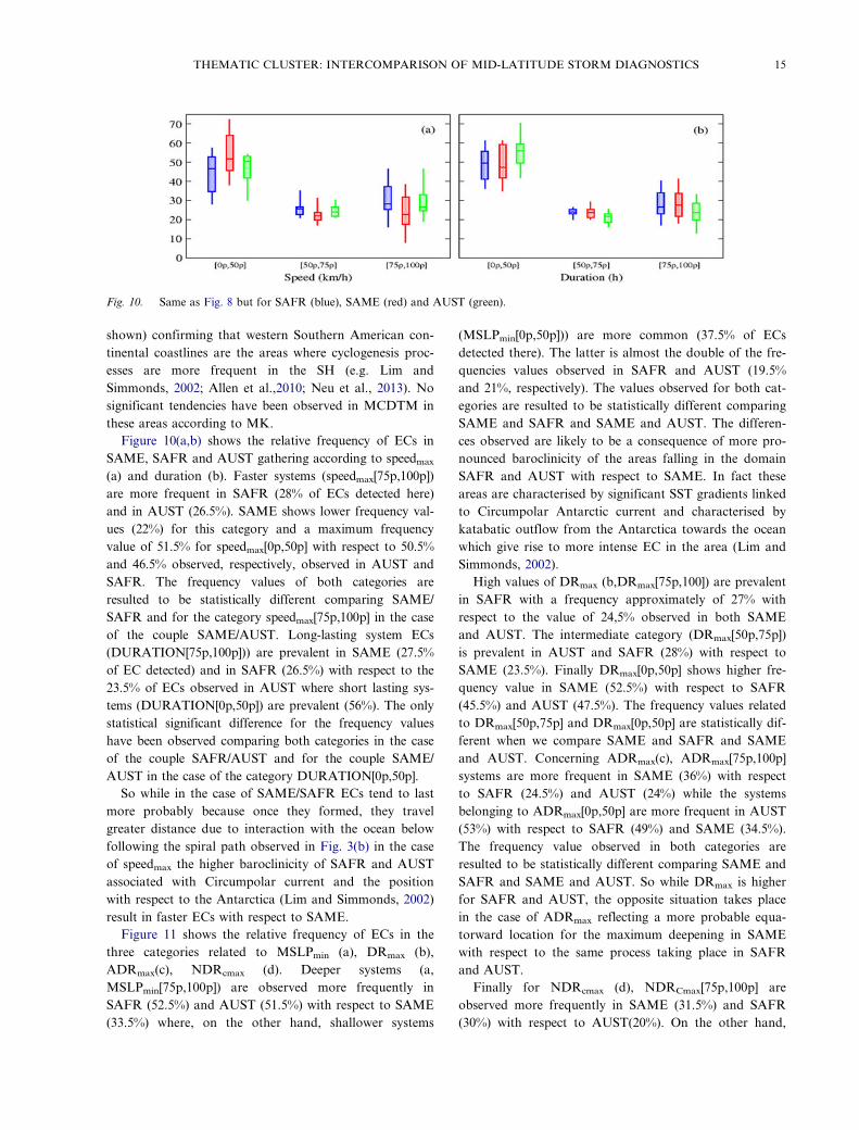
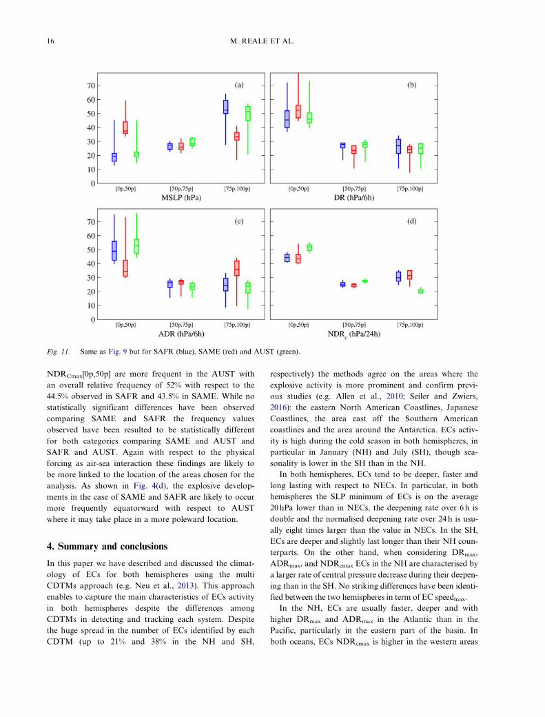
Figure 11 shows the relative frequency of ECs in thethree categories related to MSLPmin (a), DRmax (b),ADRmax(c), NDRcmax (d). Deeper systems (a,MSLPmin[75p,100p]) are observed more frequently inSAFR (52.5%) and AUST (51.5%) with respect to SAME(33.5%) where, on the other hand, shallower systems
(MSLPmin[0p,50p])) are more common (37.5% of ECsdetected there). The latter is almost the double of the fre-quencies values observed in SAFR and AUST (19.5%and 21%, respectively). The values observed for both cat-egories are resulted to be statistically different comparingSAME and SAFR and SAME and AUST. The differen-ces observed are likely to be a consequence of more pro-nounced baroclinicity of the areas falling in the domainSAFR and AUST with respect to SAME. In fact theseareas are characterised by significant SST gradients linkedto Circumpolar Antarctic current and characterised bykatabatic outflow from the Antarctica towards the oceanwhich give rise to more intense EC in the area (Lim andSimmonds, 2002).
High values of DRmax (b,DRmax[75p,100]) are prevalentin SAFR with a frequency approximately of 27% withrespect to the value of 24,5% observed in both SAMEand AUST. The intermediate category (DRmax[50p,75p])is prevalent in AUST and SAFR (28%) with respect toSAME (23.5%). Finally DRmax[0p,50p] shows higher fre-quency value in SAME (52.5%) with respect to SAFR(45.5%) and AUST (47.5%). The frequency values relatedto DRmax[50p,75p] and DRmax[0p,50p] are statistically dif-ferent when we compare SAME and SAFR and SAMEand AUST. Concerning ADRmax(c), ADRmax[75p,100p]systems are more frequent in SAME (36%) with respectto SAFR (24.5%) and AUST (24%) while the systemsbelonging to ADRmax[0p,50p] are more frequent in AUST(53%) with respect to SAFR (49%) and SAME (34.5%).The frequency value observed in both categories areresulted to be statistically different comparing SAME andSAFR and SAME and AUST. So while DRmax is higherfor SAFR and AUST, the opposite situation takes placein the case of ADRmax reflecting a more probable equa-torward location for the maximum deepening in SAMEwith respect to the same process taking place in SAFRand AUST.
Finally for NDRcmax (d), NDRCmax[75p,100p] areobserved more frequently in SAME (31.5%) and SAFR(30%) with respect to AUST(20%). On the other hand,
Fig. 10. Same as Fig. 8 but for SAFR (blue), SAME (red) and AUST (green).
THEMATIC CLUSTER: INTERCOMPARISON OF MID-LATITUDE STORM DIAGNOSTICS 15
NDRCmax[0p,50p] are more frequent in the AUST withan overall relative frequency of 52% with respect to the44.5% observed in SAFR and 43.5% in SAME. While nostatistically significant differences have been observedcomparing SAME and SAFR the frequency valuesobserved have been resulted to be statistically differentfor both categories comparing SAME and AUST andSAFR and AUST. Again with respect to the physicalforcing as air-sea interaction these findings are likely tobe more linked to the location of the areas chosen for theanalysis. As shown in Fig. 4(d), the explosive develop-ments in the case of SAME and SAFR are likely to occurmore frequently equatorward with respect to AUSTwhere it may take place in a more poleward location.
4. Summary and conclusions
In this paper we have described and discussed the climat-ology of ECs for both hemispheres using the multiCDTMs approach (e.g. Neu et al., 2013). This approachenables to capture the main characteristics of ECs activityin both hemispheres despite the differences amongCDTMs in detecting and tracking each system. Despitethe huge spread in the number of ECs identified by eachCDTM (up to 21% and 38% in the NH and SH,
respectively) the methods agree on the areas where theexplosive activity is more prominent and confirm previ-ous studies (e.g. Allen et al., 2010; Seiler and Zwiers,2016): the eastern North American Coastlines, JapaneseCoastlines, the area east off the Southern Americancoastlines and the area around the Antarctica. ECs activ-ity is high during the cold season in both hemispheres, inparticular in January (NH) and July (SH), though sea-sonality is lower in the SH than in the NH.
In both hemispheres, ECs tend to be deeper, faster andlong lasting with respect to NECs. In particular, in bothhemispheres the SLP minimum of ECs is on the average20hPa lower than in NECs, the deepening rate over 6 h isdouble and the normalised deepening rate over 24h is usu-ally eight times larger than the value in NECs. In the SH,ECs are deeper and slightly last longer than their NH coun-terparts. On the other hand, when considering DRmax,ADRmax, and NDRcmax ECs in the NH are characterised bya larger rate of central pressure decrease during their deepen-ing than in the SH. No striking differences have been identi-fied between the two hemispheres in term of EC speedmax.
In the NH, ECs are usually faster, deeper and withhigher DRmax and ADRmax in the Atlantic than in thePacific, particularly in the eastern part of the basin. Inboth oceans, ECs NDRcmax is higher in the western areas
Fig. 11. Same as Fig. 9 but for SAFR (blue), SAME (red) and AUST (green).
16 M. REALE ET AL.
than in the eastern areas. In fact, in the western areas ofthe oceans the explosive processes are strongest, as theyare characterised by strong horizontal SST gradients(Lim and Simmonds, 2002; Allen et al., 2010; Neu et al.,2013; Seilers and Zwiers, 2016) and strong air-sea inter-action, which fuels explosive developments. These differ-ences are statistically significant in particular comparingWestern Atlantic to Western Pacific and Eastern Atlanticto Eastern Pacific (for MSLPmin, DRmax, ADRmax, speed-
max), and comparing Western Atlantic to Eastern Atlantic(for the MSLPmin). On this respect, the ECs in the fourareas, at least for the extreme categories, can be consid-ered as belonging to the different populations.
In the SH, ECs close to Southern Africa and Australiaare usually faster, deeper and with higher DRmax withrespect to those close to southern South America, andECs close to southern South America and SouthernAfrica are characterised by higher NDRCmax and dur-ation with respect to ECs close to Australia. Also thesedifferences are statistically significant in particular for theextreme categories, showing that for the metrics chosenthese systems can be considered as belonging to differentpopulations.
This work has confirmed the importance of multiCDTMs approach in identifying and characterising cyc-lone activity, because of prominent differences amongthe methods.
NOTES
1. rl where r is the standard deviation and l isthe mean
MR is grateful to European Meteorological Society forits Young Scientist Travel Awards and for allowing theauthor to attend the EMS meeting in Dublin inSeptember 2017. JGP thanks the AXA research fundfor support.
Funding
This work was supported by OGS and CINECA underHPC-TRES program [grant number 2015-07 to MR]; theproject WEx-Atlantic [grant number PTDC/CTA-MET/29233/2017 to MLRL]; and Instituto Dom Luiz fundedby Fundac~ao para a Ciencia e a Tecnologia, Portugal(FCT) and Portugal Horizon 2020 [grant number UID/GEO/50019/2013].
References
Allen, J. T., Pezza, A. B. and Black, M. T. 2010. Explosivecyclogenesis: a global climatology comparing multiplereanalyses. J. Clim. 23, 6468–6484. doi:10.1175/2010JCLI3437.1
Akperov, M. G., Bardin, M. Y., Volodin, E. M., Golitsyn, G. S.and Mokhov, I. I. 2007. Probability distributions for cyclonesand anticyclones from the NCEP/NCAR reanalysis data andthe INM-RAS climate model. Izvestiya. Atmos. Ocean. Phys.43, 705–712. doi:10.1134/S0001433807060047
Bardin, M. Y. and Polonsky, A. B. 2005. North Atlanticoscillation and synoptic variability in the European-Atlanticregion in winter, Izvestiya. Atmos. Ocean. Phys. 41, 127–136.
Chang, E. K., Lee, S. and Swanson, K. L. 2002. Storm trackdynamics. J Clim 15, 2163–2183.
Chen, S. J., Kuo, Y. H., Zhang, P. Z. and Bai, Q. F. 1992.Climatology of explosive cyclones off the east Asian coast.Mon. Wea. Rev. 120, 3029–3035. doi:10.1175/1520-0493(1992)120<3029:COECOT>2.0.CO;2
De Zolt, S., Lionello, P., Malguzzi, P., Nuhu, A. and Tomasin,A. 2006. The disastrous storm of 4 November 1966 on Italy.Nat. Hazards. Earth. Syst. Sci. 6, 861–879. doi:10.5194/nhess-6-861-2006
Flaounas, E., Kelemen, F. D., Wernli, H., et al. 2016.Assessment of an ensemble of ocean–atmosphere coupled anduncoupled regional climate models to reproduce theclimatology of Mediterranean cyclones. Clim. Dyn. 51,1023–1040.
Fink, A. H., Br€ucher, T., Ermert, V., Kr€uger, A. and Pinto,J. G. 2009. The European storm Kyrill in January 2007:Synoptic evolution and considerations with respect to climatechange. Nat. Hazards Earth Syst. Sci. 9, 405–423. doi:10.5194/nhess-9-405-2009
Fink, A. H., Pohle, S., Pinto, J. G. and Knippertz, P. 2012.Diagnosing the influence of diabatic processes on theexplosive deepening of extratropical cyclones. Geophys. Res.Lett. 39, L07803.1–L07803.8.
G�omara, I., Rodr�ıguez-Fonseca, B., Zurita-Gotor, P. and Pinto,J. G. 2014. On the relation between explosive cyclonesaffecting Europe and the North Atlantic Oscillation. Geophys.Res. Lett. 41, 2182–2190. doi:10.1002/2014GL059647
Gyakum, J. R., Anderson, J. R., Grumm, R. H. and Gruner,E. L. 1989. North Pacific cold-season surface cyclone activity:1975–1983. Mon. Wea. Rev. 117, 1141–1155. doi:10.1175/1520-0493(1989)117<1141:NPCSSC>2.0.CO;2
Grieger, J., Leckebusch, G., C., Raible, C., Rudeva, I. andSimmonds, I. 2018. Subantarctic cyclones identified by 14tracking methods, and their role for moisture transports intothe continent. Tellus A: Dynamic Meteorology andOceanography 70, 1. doi:10.1080/16000870.2018.1454808
Hewson, T. D. 1997. Objective identification of frontal wavecyclones. Meteorol. App. 4, 311–315. doi:10.1017/S135048279700073X
Hewson, T. D. and Titley, H. A. 2010. Objective identification,typing and tracking of the complete life-cycles of cyclonicfeatures at high spatial resolution. Met. Apps. 17, 355–381.doi:10.1002/met.204
THEMATIC CLUSTER: INTERCOMPARISON OF MID-LATITUDE STORM DIAGNOSTICS 17
Hewson, T. and Neu, U. 2015. Cyclones, windstorms and theIMILAST project. Tellus A: Dynamic Meteorology andOceanography 67, 27128. doi:10.3402/tellusa.v67.27128
Hoskins, B. and Hodges, K. 2005. A new perspective onSouthern Hemisphere storm tracks. J. Climate, 18, 4108–4129.
Kouroutzoglou, J., Flocas, H. A., Keay, K., Simmonds, I. andHatzaki, M. 2011. Climatological aspects of explosivecyclones in the Mediterranean. Int. J. Climatol. 31,1785–1802. doi:10.1002/joc.2203
Kuwano-Yoshida, A. and Asuma, Y. 2008. Numerical study ofexplosively developing extratropical cyclones in theNorthwestern Pacific region. Mon. Wea. Rev. 136, 712–740.doi:10.1175/2007MWR2111.1
Kuwano-Yoshida, A. and Enomoto, T. 2013. Predictability ofExplosive Cyclogenesis over the Northwestern Pacific RegionUsing Ensemble Reanalysis. Mon. Wea. Rev. 141, 3769–3785.doi:10.1175/MWR-D-12-00161.1
Liberato, M. L. R., Pinto, J. G., Trigo, I. F. and Trigo, R. M.2011. Klaus – an exceptional winter storm over northernIberia and southern France. Weather 66, 330–334. doi:10.1002/wea.755
Liberato, M. L. R. 2014. The 19 January 2013 windstorm overthe North Atlantic: large-scale dynamics and impacts onIberia. Weather Clim. Extremes 5, 16–28.
Lim, E. and Simmonds, I. 2002. Explosive cyclone developmentin the Southern Hemisphere and a comparison with NorthernHemisphere events. Mon. Wea. Rev. 130, 2188–2209. doi:10.1175/1520-0493(2002)130<2188:ECDITS>2.0.CO;2
Lionello, P., Dalan, F. and Elvini, E. 2002. Cyclones in theMediterranean region: the present and the doubled CO2climate scenarios. Clim. Res. 22, 147–159. doi:10.3354/cr022147
Lionello, P. et al. 2016. Objective climatology of cyclones in theMediterranean region: a consensus view among methods withdifferent system identification and tracking criteria. Tellus:Series A, Dynamic Meteorology and Oceanography, 68, 1–18.
Ludwig, P., Pinto, J. G., Reyers, M. and Gray, S. L. 2014. Therole of anomalous SST and surface fluxes over thesoutheastern North Atlantic in the explosive development ofwindstorm Xynthia. Qjr. Meteorol. Soc. 140, 1729–1741. doi:10.1002/qj.2253
Murray, R. J. and Simmonds, I. 1991. A numerical scheme fortracking cyclone centers from digital data. Part I:development and operation of the scheme. Aust. Meteorol.Mag 39, 155–166.
Neu, U., Akperov, M. G., Bellenbaum, N., Benestad, R., Blender,R. et al. 2013. IMILAST-a community effort to intercompareextratropical cyclone detection and tracking algorithms:assessing method-related uncertainties. Bull. Amer. Meteor.Soc. 94, 529–547. doi:10.1175/BAMS-D-11-00154.1
Nissen, K. M., Leckebusch, G. C., Pinto, J. G., Renggli, D.,Ulbrich, S. et al. 2010. Cyclones causing wind storms in theMediterranean: characteristics, trends and links to largescalepatterns. Nat. Hazards Earth Syst. Sci. 10, 1379–1391. doi:doi:10.5194/nhess-10-1379-2010
Peixoto, J. P. and Oort, A. H. 1992. Physics of Climate.Springer, Berlin.
Pinto, J. G., Spangehl, T., Ulbrich, U. and Speth, P. 2005.Sensitivities of a cyclone detection and tracking algorithm:individual tracks and climatology. Metz. 14, 823–838. doi:10.1127/0941-2948/2005/0068
Pinto, J. G., Ulbrich, S., Parodi, A., Rudari, R., Boni, G. et al.2013. Identification and ranking of extraordinary rainfallevents over Northwest Italy: the role of Atlantic moisture. J.Geophys. Res. Atmos. 118, 2085–2097. doi:10.1002/jgrd.50179
Pinto, J. G., Ulbrich, S., Economou, T., Stephenson, D. B.,Karremann, M. K. et al. 2016. Robustness of serial clusteringof extratropical cyclones to the choice of tracking method.Tellus A: Dynamic Meteorology and Oceanography 68, 32204.doi:10.3402/tellusa.v68.32204
Raible, C. C. 2007. On the relation between extremes of midaltitude cyclones and the atmospheric circulation usingERA40. Geophys. Res. Lett., 34, L07703.1–L07703.6
Roebber, P. J. 1984. Statistical analysis and updated climatologyof explosive cyclones. Mon. Wea. Rev. 112, 1577–1589. doi:10.1175/1520-0493(1984)112<1577:SAAUCO>2.0.CO;2
Rudeva, I., Gulev, S. K., Simmonds, I. and Tilinina, N. 2014.The sensitivity of characteristics of cyclone activity toidentification procedures in tracking algorithms. Tellus A 66,24961. doi:10.3402/tellusa.v66.24961
Reale, M. and Lionello, P. 2013. Synoptic climatology of winterintense precipitation events along the Mediterranean coasts.Nat. Hazards Earth Syst. Sci. 13, 1707–1722. doi:10.5194/nhess-13-1707-2013
Sanders, F. and Gyakum, J. R. 1980. Synoptic-dynamicclimatology of the bomb. Mon. Wea. Rev. 108, 1589–1606.doi:10.1175/1520-0493(1980)108<1589:SDCOT>2.0.CO;2
Sanders, F. 1986. Explosive cyclogenesis in the west-centralNorth Atlantic Ocean, 1981-84. Part I: Composite structureand mean behavior. Mon. Wea. Rev. 114, 1781–1794. doi:10.1175/1520-0493(1986)114<1781:ECITWC>2.0.CO;2
Seiler, C. and Zwiers, F. W. 2016. How well do CMIP5 climatemodels reproduce explosive cyclones in the extratropics of theNorthern Hemisphere? Clim. Dyn. 46, 1241. doi:10.1007/s00382-015-2642-x
Serreze, M. C. 1995. Climatological aspects of cyclonedevelopment and decay in the Arctic. Atmos. Ocean 33, 1–23.doi:10.1080/07055900.1995.9649522
Stull, R. B. 2000. Meteorology for Scientists and Engineers: A
Technical Companion Book with Ahrens’ Meteorology Today,Pacific Grove,CA: Brooks/Cole.
Simmonds, I., Burke, C. and Keay, K. 2008. Arctic climatechange as manifest in cyclone behavior. J. Clim. 21,5777–5796. doi:10.1175/2008JCLI2366.1
Trigo, I. F. 2006. Climatology and interannual variability ofstorm tracks in the Euro-Atlantic sector: a comparisonbetween ERA- 40 and NCEP/NCAR reanalyses. Clim. Clim.
Dyn. 26, 127–143. doi:10.1007/s00382-005-0065-9Ulbrich, U., Leckebusch, G. C., Grieger, J., et al. 2013. Are
Greenhouse Gas Signals of Northern Hemisphere winterextra-tropical cyclone activity dependent on theidentification and tracking algorithm? Meteor. Z. 22, 61–68.doi:10.1127/0941-2948/2013/0420
Wang, X. L., Swail, V. R. and Zwiers, F. W. 2006. Climatologyand changes of extra-tropical cyclone activity: comparison ofERA-40 with NCEP/NCAR reanalysis for 1958-2001. J. Clim.19, 314–3166.
Wang, C. and Rogers, J. C. 2001. A composite study of explosivecyclogenesis in different sectors of the north Atlantic. Part i:
cyclone structure and evolution.Mon. Wea. Rev. 129, 1481–1499.doi:10.1175/1520-0493(2001)129<1481:ACSOEC>2.0.CO;2
Wernli, H. and Schwierz, C. 2006. Surface cyclones in the ERA-40data set (1958-2001). Part I: novel identification method andglobal climatology. J. Atmos. Sci. 63, 2486–2507. doi:10.1175/JAS3766.1
THEMATIC CLUSTER: INTERCOMPARISON OF MID-LATITUDE STORM DIAGNOSTICS 19