A Global Hindcast of Ice and OceanA Global Hindcast of Ice and OceanConditions for 1958-2004Conditions for 1958-2004

(with a Focus on the North Atlantic and Arctic)(with a Focus on the North Atlantic and Arctic)

W. Paul BudgellW. Paul Budgellandand

Vidar S. LienVidar S. Lien

Institute of Marine ResearchInstitute of Marine Researchandand

Bjerknes Centre for Climate ResearchBjerknes Centre for Climate ResearchBergen, NorwayBergen, Norway

AlcalAlcaláá de Henares de HenaresNovember 6-8, 2006November 6-8, 2006

IMR

IMR

Outline of Talk:Outline of Talk:

• BackgroundBackground

• Description of ice-ocean model Description of ice-ocean model

• Model set-upModel set-up

• Preliminary simulation resultsPreliminary simulation results • ConclusionsConclusions

IMR

BackgroundBackground

• Performing global ice-ocean forecast for Performing global ice-ocean forecast for 1958-20041958-2004

• Archived hindcast results used to run Archived hindcast results used to run ecosystem model off-line and generate ecosystem model off-line and generate time series of biophysical/indicators for time series of biophysical/indicators for fisheries-climate studiesfisheries-climate studies

• Global to provide dynamically-consistent Global to provide dynamically-consistent fields for boundary forcing of regional fields for boundary forcing of regional modelsmodels

IMR

Ocean Model Component (ROMS v. 3.0)Ocean Model Component (ROMS v. 3.0)

• 3rd-order upwind-biased horizontal advection3rd-order upwind-biased horizontal advection

• Piece-wise parabolic splines in vertical, spline Piece-wise parabolic splines in vertical, spline vertical advection, spline Jacobian baroclinic vertical advection, spline Jacobian baroclinic pressure gradient at topographypressure gradient at topography

• LMD mixing with bottom PBL extensionLMD mixing with bottom PBL extension

• Global tides with tidal potential and Global tides with tidal potential and SAL correctionSAL correction

• Atmospheric pressure gradient forcingAtmospheric pressure gradient forcing

Ice DynamicsIce Dynamics

• Ice dynamics based upon the elastic-viscous-plastic Ice dynamics based upon the elastic-viscous-plastic (EVP) rheology of Hunke and Dukowicz (1997), Hunke (EVP) rheology of Hunke and Dukowicz (1997), Hunke (2001) and Hunke and Dukowicz (2002)(2001) and Hunke and Dukowicz (2002)

• Under low deformation (rigid behaviour), the Under low deformation (rigid behaviour), the singularity is regularized by elastic wavessingularity is regularized by elastic waves– response is very similar to viscous-plastic models in response is very similar to viscous-plastic models in

typical Arctic pack ice conditionstypical Arctic pack ice conditions

• Numerical behaviour improved significantly by Numerical behaviour improved significantly by applying linearization of the viscosities at every EVP applying linearization of the viscosities at every EVP time steptime step

• The EVP model parallelizes very efficiently under both The EVP model parallelizes very efficiently under both OpenMP And MPIOpenMP And MPI

IMR

IMR

Ice ThermodynamicsIce Thermodynamics

Ice thermodynamics are based upon those of Ice thermodynamics are based upon those of Mellor and Kantha (1989) and Häkkinen and Mellor and Kantha (1989) and Häkkinen and Mellor (1992)Mellor (1992)

Main features include:Main features include:• Three-level, single layer ice; single snow layerThree-level, single layer ice; single snow layer• Molecular sublayer under ice; Prandtl-type ice-ocean Molecular sublayer under ice; Prandtl-type ice-ocean boundary layerboundary layer• Surface melt ponds; enthalpy conservationSurface melt ponds; enthalpy conservation• Forcing by short and long-wave radiation, sensible Forcing by short and long-wave radiation, sensible and latent heat fluxand latent heat flux• Tight coupling to ocean surface boundary layerTight coupling to ocean surface boundary layer

IMR

Model GridModel Grid

Every 10Every 10thth point in i,j directions plotted point in i,j directions plotted

IMR

Model Grid SizeModel Grid Size

Model Set-upModel Set-up

• Horizontal resolution of 8.9 to 105 km, Horizontal resolution of 8.9 to 105 km, average of 20 km in N. Atlantic and average of 20 km in N. Atlantic and Arctic on a stretched spherical grid with Arctic on a stretched spherical grid with Mercator projectionMercator projection

• 35 levels in the vertical, stretched for 35 levels in the vertical, stretched for enhanced resolution in the surface enhanced resolution in the surface mixed layer, mixed layer, ΘΘss=5.0, =5.0, ΘΘbb=0.4, h=0.4, hminmin=30m=30m

IMR

IMR

Initial Conditions and ForcingInitial Conditions and Forcing

• Initial condition in Jan.1, 1958 from Jan.1, 2001 Initial condition in Jan.1, 1958 from Jan.1, 2001 from NERSC MICOM global hindcast from 1948-from NERSC MICOM global hindcast from 1948-2001, then 2 years of forcing with CORE 2001, then 2 years of forcing with CORE corrected normal yearcorrected normal year

• CORE (Common Ocean-ice Reference CORE (Common Ocean-ice Reference Experiment) data set used for forcing; surface Experiment) data set used for forcing; surface heat and momentum fluxes computed using heat and momentum fluxes computed using COARDS 3.0 bulk flux algorithms in ROMSCOARDS 3.0 bulk flux algorithms in ROMS

• Restoration of sea surface salinity to Restoration of sea surface salinity to climatology with 90 day e-folding timeclimatology with 90 day e-folding time

Spin-Up Still Required!Spin-Up Still Required!

IMR

Results – SST - MarchResults – SST - March

Observed Climatology Observed Climatology MarchMarch

(Pathfinder)(Pathfinder)

Model resultsModel resultsMarch, 2004March, 2004

IMR

Results – SST - Results – SST - SeptemberSeptember

Observed Climatology Observed Climatology SeptemberSeptember(Pathfinder)(Pathfinder)

Model resultsModel resultsSeptember, 2004September, 2004

IMR

IMR

Observed (SMM/R)Observed (SMM/R) ModelledModelled

Daily Mean Ice Concentration Daily Mean Ice Concentration March 20, 1980March 20, 1980

IMR

Observed (SMM/R)Observed (SMM/R) ModelledModelled

Daily Mean Ice Concentration Daily Mean Ice Concentration Sept.19, 1980Sept.19, 1980

IMR

March, 1980March, 1980 September, 1980September, 1980

Modelled Modelled Monthly Mean Sea Ice Thickness (m)Monthly Mean Sea Ice Thickness (m)

Preliminary Results - Preliminary Results - SectionsSections

IMR

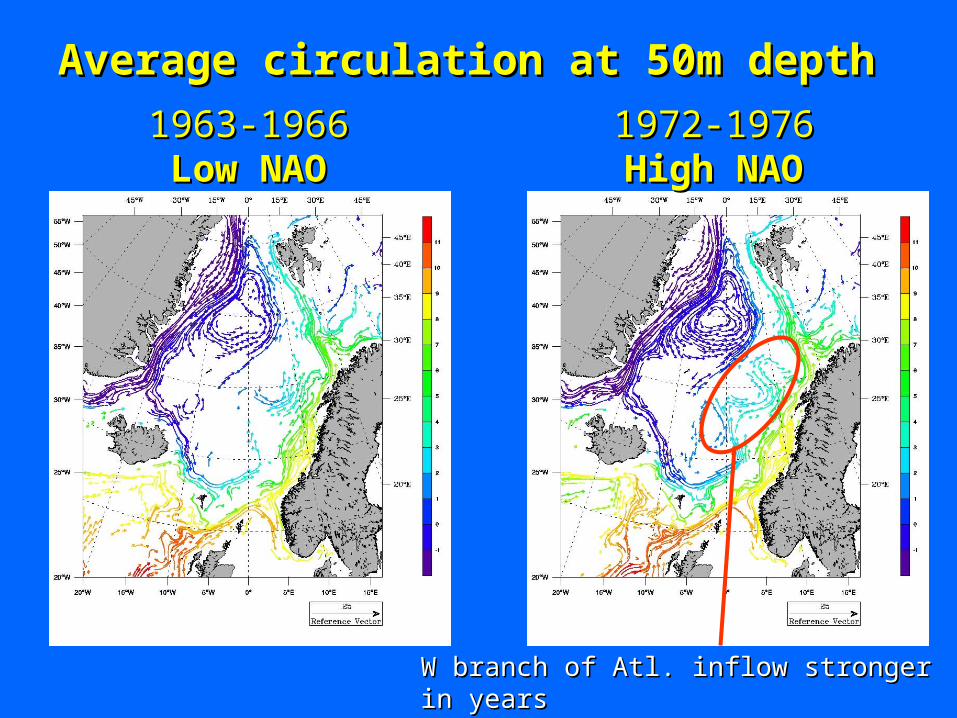
Northward Velocity at 66Northward Velocity at 66ººN and the N and the NAONAO

Low NAO High NAO Low NAO

1963-19661963-1966Low NAOLow NAO

1972-19761972-1976High NAOHigh NAO

Average circulation at 50m depthAverage circulation at 50m depth

W branch of Atl. inflow stronger in yearsW branch of Atl. inflow stronger in yearswith high NAO-index (i.e. more SW with high NAO-index (i.e. more SW winds)winds)

Section at the Barents OpeningSection at the Barents Opening50-200m average from 7150-200m average from 71°°30’N to 7330’N to 73°°30’N30’N

Observations (1977-Observations (1977-04)04)

Model results (1977-Model results (1977-04)04)

mean mean salinitysalinity

temperaturetemperature

35.0535.05

34.9934.995.29 5.29 ººC C

4.90 4.90 ººCC

Atlantic Inflow Atlantic Inflow (Mooring “sampling”)(Mooring “sampling”)

Observed (AW net, 1997-2001): 1.5 Sv Observed (AW net, 1997-2001): 1.5 Sv Modelled (AW net, 1997-2001): 1.8 Sv Modelled (AW net, 1997-2001): 1.8 Sv

IMR

IMR

Bering Strait Transport to the ArcticBering Strait Transport to the Arctic

Modelled: 1.15 SvModelled: 1.15 Sv

Woodgate: 0.8 SvWoodgate: 0.8 Sv

Roach: 0.83 SvRoach: 0.83 Sv

Clement: 0.65 SvClement: 0.65 Sv(Modelled)(Modelled)

IMR

Southward Labrador Current TransportSouthward Labrador Current Transport

Modelled DSOModelled DSOTransport = Transport = 13-14 Sv13-14 Sv

Observed DSO TransObserved DSO Trans(Fischer et al., 2004)(Fischer et al., 2004)13.8 Sv.13.8 Sv.

Modelled LSW TransModelled LSW Trans= = ~11-12 Sv~11-12 Sv

Obs LSW TransObs LSW Trans(Fischer et al., 2004)(Fischer et al., 2004)==11.4 Sv11.4 Sv

IMR

Fram Strait TransportFram Strait Transport

Modelled Northward Transport = Modelled Northward Transport = 9.0 Sv9.0 Sv

Observed Northward Transport = Observed Northward Transport = 9 +/- 2 Sv9 +/- 2 Sv(Schauer et al., 2004)(Schauer et al., 2004)

Modelled Southward Transport = Modelled Southward Transport = 12.9 Sv12.9 Sv

Observed Southward Transport = Observed Southward Transport = 13 +/- 2 Sv13 +/- 2 Sv

IMR

East Greenland Current TransportEast Greenland Current Transport

Modelled Average Southward Trans = Modelled Average Southward Trans = 25.1 Sv25.1 Sv

Observed Average Southward Trans = Observed Average Southward Trans = 21 +/- 3 Sv21 +/- 3 Sv(Woodgate et al., 1999)(Woodgate et al., 1999)

Net Atlantic Water Southward Trans = Net Atlantic Water Southward Trans = 8.8 Sv8.8 Sv

Net Atlantic Water Southward Trans = Net Atlantic Water Southward Trans = 8 +/- 1 Sv8 +/- 1 Sv(Woodgate et al., 1999)(Woodgate et al., 1999)

IMR

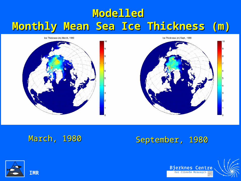
Animations of Annual VariabilityAnimations of Annual Variability

Results are shown from the first year of a Results are shown from the first year of a global simulation starting in 2001 using global simulation starting in 2001 using NCEP flux forcingNCEP flux forcing

Initialized from coarse MICOM hindcast of Initialized from coarse MICOM hindcast of 1948-20001948-2000

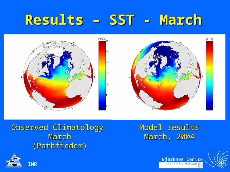
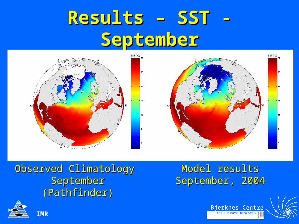
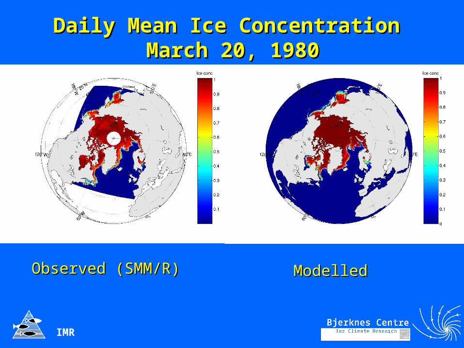
SST Ice Concentration

IMR

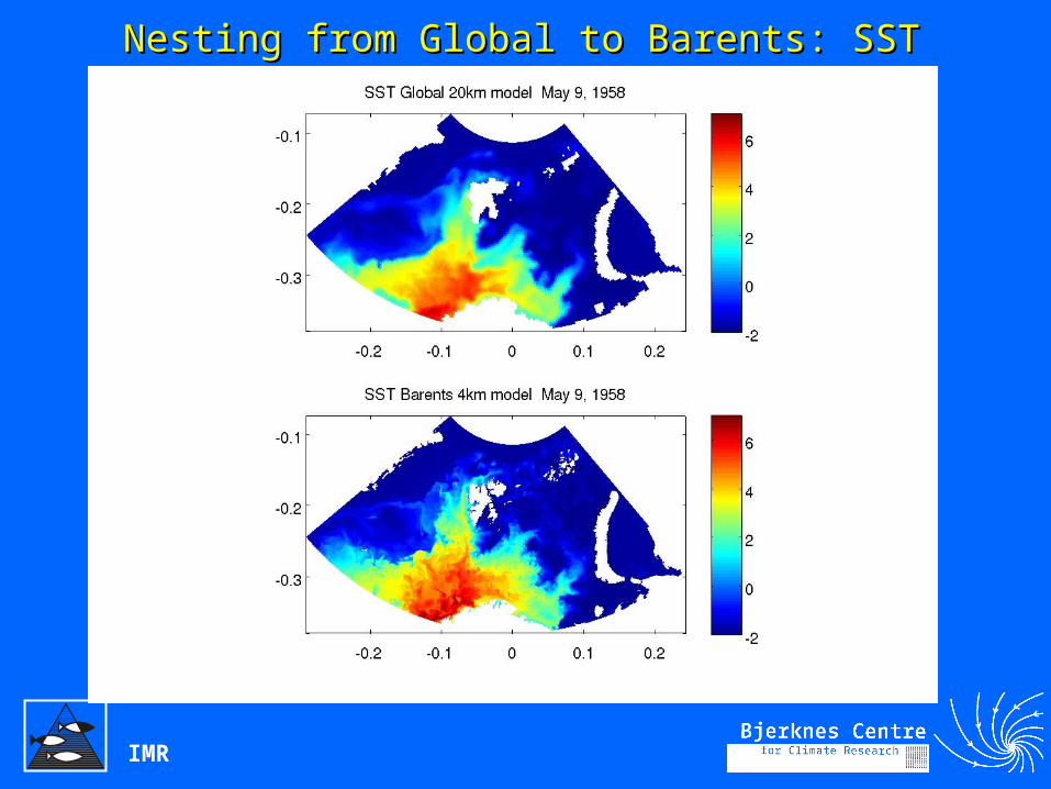
Nesting from Global to Barents: SSTNesting from Global to Barents: SST

IMR

Nesting from Global to Barents: Nesting from Global to Barents: Surface CurrentsSurface Currents

IMR

Storfjorden Storfjorden Mesoscale Ice-Ocean InteractionMesoscale Ice-Ocean Interaction

IMR

Summary and ConclusionsSummary and Conclusions

• The first pass of a global ice-ocean hindcast has The first pass of a global ice-ocean hindcast has been completed for 1958-2004 and data are archived been completed for 1958-2004 and data are archived as 3-day and monthly meansas 3-day and monthly means

• The results are not spun up in the deep ocean until The results are not spun up in the deep ocean until the early 1980’sthe early 1980’s

• The results generally look reasonable and time The results generally look reasonable and time series are being analyzed for interannual & decadal-series are being analyzed for interannual & decadal-scale variabilityscale variability

• Archived hindcast fields are being used for nesting Archived hindcast fields are being used for nesting of regional models and in off-line IBM simulations of of regional models and in off-line IBM simulations of zooplankton and fish larvae simulations, and off-line zooplankton and fish larvae simulations, and off-line ecosystem simulationsecosystem simulations

IMR

Future WorkFuture Work

• Problems with anomalous cold patches off Argentina Problems with anomalous cold patches off Argentina and in the central North Atlantic – probably due to and in the central North Atlantic – probably due to errors in w-computation (pers.comm. Daniel Deacu, errors in w-computation (pers.comm. Daniel Deacu, Memorial Univ., NL, Canada)Memorial Univ., NL, Canada)

• Will repeat the hindcast from Jan., 1958 initialized Will repeat the hindcast from Jan., 1958 initialized from Jan., 1996; SSS restoration will be replaced with from Jan., 1996; SSS restoration will be replaced with spectral (12-month and long-term mean) correction of spectral (12-month and long-term mean) correction of surface salt flux based on archived salinity restoration surface salt flux based on archived salinity restoration flux time series from the first runflux time series from the first run

• “ “Potential vorticity barrier” inhibits Atlantic inflow to Potential vorticity barrier” inhibits Atlantic inflow to the Nordic Seas; need to find a suitable the Nordic Seas; need to find a suitable parameterizationparameterization