A Goal Programming Model for Capital Rationing with a ...

Journal of Administrative Sciences And Economics Vol. 8-1997

A Goal Programming Model for Capital Rationing with a Linear

Cash Fluctuations Measure

Dr. M. Asaad Elnidani

Business Administration Department College of Management and Technology

Arab Academy for Science and Technology And Maritime Transport

17


A GOAL PROGRAMMING MODEL FOR CAPITAL

RATIONING WITH A LINEAR CASH FLUCTUATIONS

MEASURE 1- Introduction

Capital rationing arise in situations where the total available

resources (capital, labor, materials, etc.) is less than the resource

requirements for all investment opportunities being considered by

management [1]. Therefore firms need to devise procedures for

rationing in order to select the optimal group(ll of investments under

the restriction of scarce resources. Several capital rationing techniques

for the ranking of alternatives is presented in the literature [1-3].

Most of these approaches will provide good means of ranking

the alternatives. Put this way, management then selects from the list

until either the list or the available resources is exhausted. Optimality

is not guaranteed through this procedure. Consider the following

example.

Example 1

Consider Table (1) below:

Proposal

Capital

NPV

1 2

20,000 12,000

4,000

Table (1)

Example 1 data

2,500

3

9,000

2,200

Note that investment proposals are ranked according to the

values of the Net Present Value (NPV). If the capital available is

(l) Optimality is considered with respect to the objective function being evaluated. Different objectives in most cases will yield different optimal groups.

19

A Goal Programming Model for Capital Rationing Dr. M. Asaad Elnidani

25,000 then only the first alternative will be selected. In this case a

total NPV of 4,000 is realized. If on the other hand, investment

opportunities 2 and 3 are selected (total capital expenditure would be

21,000) then a total NPV of 4,700 is realized.

Other techniques as linear programming may be used. In this

case the objective function is to maximize the total NPV realized.

In many cases the need arises for achieving more than one

objective. Goal programming provided a way of realizing these

objectives simultaneously. The concept of goal programming was

initially developed in the early sixties by Charnes and Cooper [4]. In

1965, Ijiri [5] introduced additional definitions and refinements of

the technique. Several applications and extensions were later given

by Ignizio [6] and Lee [7]. The concept was applied to capital

rationing to allow for multiple objective rationing [3, 8-15].

In this paper a goal programming model is developed that

selects a group of investment opportunities which maximized the

annual cash flow fluctuations. Both objective functions are linear

mixed integer functions. Several measures of deviation are introduced,

compared, and analyzed via computer runs using RISK [16]. Test

problem were randomly generated by BUDGEN [17]. Implementation

of the model, test examples, and concluding remarks are presented.

Special constraints and cases of the capital rationing problem are

presented in Appendix A.

2- Notation

The following notation is used throughout the paper:

I .=.the set of all investments i; 0 ~ i ~ m (where i=O

represent investments).

20


3-

a.

(2)

x1 ( 1. if investment i is selecte~2l l 0. otherwise j

fij = cash flow of investment i in year j; l ~ j ~ n

Fj = annual combined cash flows of current and selected

investments in year j.

Fj = L/iJXi iel ; 1 , j , n (1)

CJ -;;- standard deviation of the combined annual cash flows of

current and selected investments.

Pi -;;- net present value of ni cash flows generated by investment

opportunity i.

CL -;;- total capital available in local currency.

CF -;;- total capital available in foreign currency.

C -;;- total capital available, irrespectful of currency.

eli -;;- capital required for proposal i in local currency.

cf; -;;- capital required for proposal i in foreign currency.

ci -;;- capital required for investment opportunity i, irrespectful

of currency.

Assumptions

The proposed model relies on the following set of assumptions:

Indivisible investment opportunities: proposed investments can

The variable x0

represents the current investments and will always equal to 1. This means, it is a constant not a variable. · Yet, to simplify the notation and the calculation of the cash fluctuation function, it will be considered a variable in the notation and will be treated as a constant in the development of the model as will be shown later.

21

A Goal Programming Model for Capital Rationing Dr. M. Asaad Elllidalli

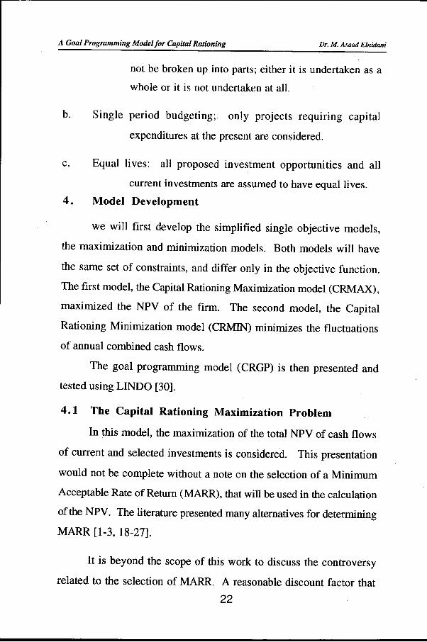
not be broken up into parts; either it is undertaken as a

whole or it is not undertaken at all.

b. Single period budgeting; only projects requiring capital

expenditures at the present are considered.

c. Equal lives: all proposed investment opportunities and all

current investments are assumed to have equal lives.

4. Model Development

we will first develop the simplified single objective models,

the maximization and minimization models. Both models will have

the same set of constraints, and differ only in the objective function.

The first model, the Capital Rationing Maximization model (CRMAX),

maximized the NPV of the firm. The second model, the Capital

Rationing Minimization model (CRMIN) minimizes the fluctuations

of annual combined cash flows.

The goal programming model ( CRGP) is then presented and

tested using LINDO [30].

4.1 The Capital Rationing Maximization Problem

In this model, the maximization of the total NPV of cash flows

of current and selected investments is considered. This presentation

would not be complete without a note on the selection of a Minimum

Acceptable Rate of Return (MARR), that will be used in the calculation

of the NPV. The literature presented many alternatives for determining

MARR [1-3, 18-27].

It is beyond the scope of this work to discuss the controversy

related to the selection of MARR. A reasonable discount factor that

22


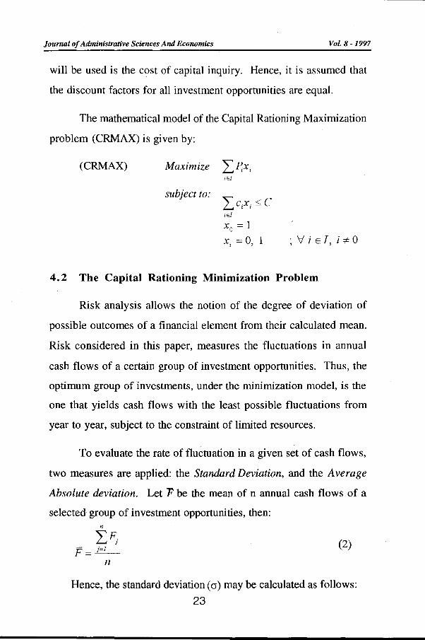
will be used is the cost of capital inquiry. Hence, it is assumed that

the discount factors for all investment opportunities are equal.

The mathematical model of the Capital Rationing Maximization

problem (CRMAX) is given by:

(CRMAX) Maximize L P;x; iEJ

subject to:

iEl

;'ViEl,i=tO

4.2 The Capital Rationing Minimization Problem

Risk analysis allows the notion of the degree of deviation of

possible outcomes of a financial element from their calculated mean.

Risk considered in this paper, measures the fluctuations in annual

cash flows of a certain group of investment opportunities. Thus, the

optimum group of investments, under the minimization model, is the

one that yields cash flows with the least possible fluctuations from

year to year, subject to the constraint of limited resources.

To evaluate the rate of fluctuation in a given set of cash flows,

two measures are applied: the Standard Deviation, and the Average

Absolute deviation. Let F be the mean of n annual cash flows of a

selected group of investment opportunities, then: n

L~ F=f!__

(2)

n

Hence, the standard deviation ( cr) may be calculated as follows:

23


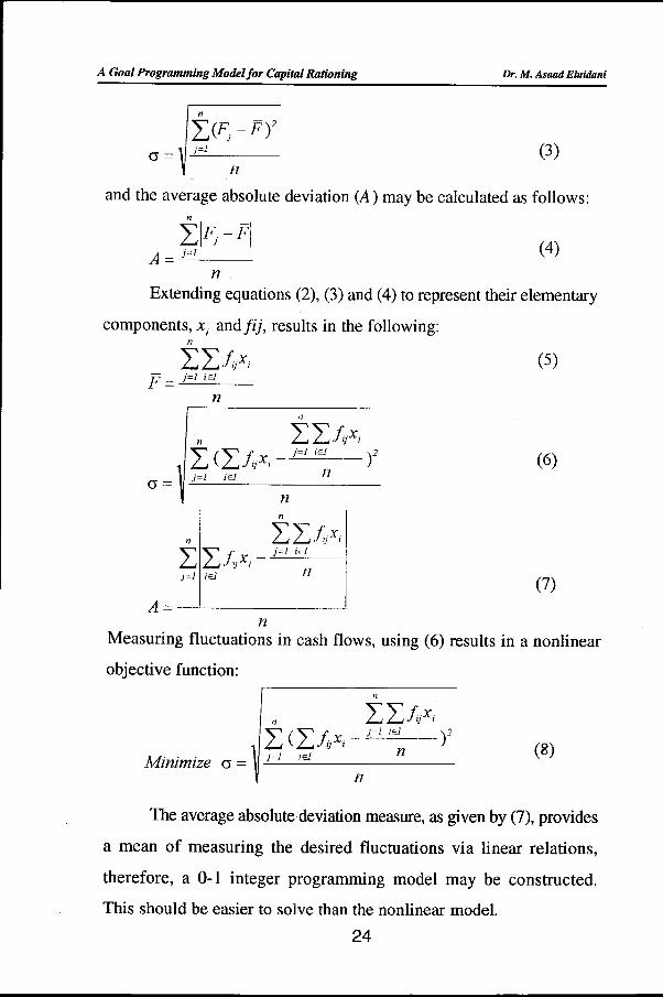
(3)

and the average absolute deviation (A) may be calculated as follows:

fiFJ-PI A = -'-i=_I ---

(4)

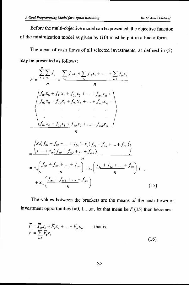
n Extending equations (2), (3) and (4) to represent their elementary

components, X; andfij, results in the following: n

L:L:J;jxi (5) p = J=l iEl

n

n

L (L/;Jxi- J=I iEI

1 J=I ;EI n a=

(6)

n

(7) A = _ _,__ _____ ____!_

n Measuring fluctuations in cash flows, using (6) results in a nonlinear

objective function:

(8)

The average absolute deviation measure, as given by (7), provides

a mean of measuring the desired fluctuations via linear relations,

therefore, a 0-1 integer programming model may be constructed.

This should be easier to solve than the nonlinear model.

24


Therefore, the objective function will take the form:

11 L. L. .f]x, - j=l iEl

;=I iEI n (9)

Minimize A = ---'----·-------'-n

The minimum value of A subject to the constraints of the

problem is equal to the minimum value of n*A subject to the same

set of constraints, therefore, (9) may be reduced to the following: n

n LLfijxi Minimize A= L Lfij- -'--j=-

1-18---1

j=l iEl n (10)

4.2.1 Comparison between the two Measures of Risk

It will be shown that the average absolute deviation model

yields results that are very close to those provided by the standard

deviation model. Because either measure simply determines how

different alternatives compare in terms of cash fluctuations, close

results are considered satisfactory for risk measurement.

It should be noted that the standard deviation does provide a

more accurate measure of dispersion (the degree to which a set of

values vary about their mean) than the average absolute deviation on

the same sets of data [28]. Therefore, it is valid to say that selections

made by the two measures, may be different. We need to answer

two questions: how much do they differ? And, how often?

The program BUDGEN [17] was used to randomly generate

hundreds of test cases. The program RISK [16] was then used to test

25


and evaluate these cases. Each case consists of a predefined number

of alternatives and their annual cash flows. The following measures

were computed:

(A) The Consecutive Absolute Difference:

n~J

L:l~ -~+11 j=l

(11)

(B) The Relative Absolute Difference:

n~I F F L: j j+l

n (12)

J=l

(C) The Average Absolute Deviation of n cash flows:

n~J

L:I~-PI (13) j=l

n

(D) The Standard Deviation ofn cash flows:

n

L(~ -F)2 (14)

\ i=I n

A group of one hundred sets of problems (cases) were generated.

Each set is composed of four investment opportunities. For each

alternative, cash flows for eight years were randomly generated.

The four measures were computed. The total number of times

where each measure selects the same alternative as the one selected

by the variance is registered. The results are summarized in Table

(2) below. 26


Number of times measure selects the same proposal as the one selected by the

Measure of Risk standard deviation A Consecutive Absolute Difference 35 B Relative Absolute Difference 22 c Average Absolute Difference 86

Table (2)

The number of times each measure selects the same

alternative as the one selected by the standard deviation

It is clear from Table (2) that the average absolute deviation

measure was much closer than the absolute and relative differences in

the selection of alternatives. The absolute difference missed 65% of

the cases and was only correct 35% of the times. The Relative

difference missed 78% of the cases and was correct 22% of the

times. Although such results may not be generalized, they are good

enough to determine that the average absolute deviation measure is

superior to the absolute and relative differences in measuring risk.

This triggers the next test.

In order to get a better feel of how close the average absolute

deviation is in selecting investment proposals as compared to the

standard deviation, a program RISKAUTO [29] was used. This

program uses data generated by BUDGEN [17], tests them using

RISK [16] and risk measure. A success is registered when a risk

measure selects the same alternative as the one selected by the standard

deviation. RISKAUTO provides three values: MINDIFF (the minimum

difference), MAXDIFF (the maximum difference), and AVGDIFF

(the average difference).

27


To illustrate, consider this example. The results of one of the

test sets with 6 investment alternatives. An alternative may consist of

more than one investment opportunity. A group of investment

opportunities that do not violate any of the problem constraints may

hence be called an investment alternative3 are shown in Table (3).

The Standard and average absolute deviation of the annual cash flows

were calculated for each alternative.

Investment Alternatives Year 1 2 3 4 5 6

1 5,000 1,000 6,000 1,500 500 5,000 2 5,600 1,500 4,500 1,000 1,400 3,000 3 4,500 100 1,500 1,400 900 5,000 4 1,800 1,500 2,800 1,800 1,500 2,000 5 500 1,500 1,200 900 800 1,500 6 1,800 2,000 1,500 1,200 1,200 2,600 7 2,000 180 6,000 1,000 700 8,000 8 1,500 200 5,000 2,000 500 7,000 9 2,000 2,000 1,000 1,200 400 5,000 10 1,500 1,000 200 1,000 600 2,000

Table (3)

Cash flows, Standard Deviation and Average Absolute

Deviation of 6 investment alternatives

According to Table (3), the best alternative according to the

standard deviation is the fourth Ccr =371), and the best alternative

according to the average absolute 'deviation is the fifth (A =290).

(3) An alternative may consist of more than one investment oppmtunity. A group on investment oppmtunities that do not violate any of the problem constraints may hence be called an investment alternative.

28


Such a case will be registered as a failure for the average absolute

deviation for selecting an alternative other than that selected by the

standard deviation. In this case, we calculate the difference between

the standard deviation of the fourth and fifth alternatives and find it

to be 2 (0.54% ). This difference is then saved and compared to

other differences for other test sets. From these differences the three

values MINDIFF, MAXDIFF and A VGDIFF are registered.

Three groups of problems were tested based on the above test

procedure. The first consisted of investment opportunities

(alternatives) with lives equal to 10 years, the second 15 years and

the third 20 years. In each group, different problem sizes were

tested, ranging from sets with 3 alternatives each, through sets with

20 alternatives each. On each problem size, 100 sets of randomly

generated problems were tested from which the three values, MIND IFF,

MAXDIFF and A VGDIFF were calculated. In addition, the total

number of successes were reported as the number of matches. A

total of 5,400 test cases were generated, tested and reported. Table

(4) below summarizes the results of these tests.

29

A Goal Programming Model for Capital Rationing Dr. M. Aslllld Elnidani

Number ot Annual cash Bows No. of Cash flows= 10 Cash flows= 15 Cash flows = 20 inv. No. ot IJJtterence No. ot IJttterence No. ot alt. mate he~ min max avg matches min max avg matches

j YO 1.29 1:1.:115 ),()4 Y3 l.'J/ . LU.45 16.54 93

4 91 1.71 13.11 3.94 86 0.43 10.99 3.18 94

5 91 1.49 9.90 3.79 92 0.04 9.64 4.30 89

6 85 0.05 14.78 6.51 84 0.32 13.34 4.51 91

7 90 0.32 15.45 4.17 88 0.38 9.37 5.58 94

8 85 1.00 27.54 7.82 84 0.14 15.11 3.82 90

9 84 0.29 10.71 5.16 90 0.16 8.14 3.41 85

10 87 0.37 20.60 5.34 85 0.37 14.41 6.05 90

11 84 0.43 26.08 9.83 87 0.01 10.94 4.55 94

12 80 0.10 17.28 6.28 89 0.01 10.72 3.59 84

13 78 1.28 22.02 8.25 75 0.11 14.63 4.28 89

14 77 0.25 91.51 6.81 82 0.59 13.04 6.21 84

15 83 0.67 17.07 9.39 86 o.oo· 12.99 6.32 84

16 81 0.03 17.53 5.87 84 0.40 12.35 4.63 85

17 82 0.10 20.62 8.20 80 0.02 9.89 4.32 79

18 74 0.06 15.40 6.35 82 0.23 10.28 4.53 78

19 79 0.06 24.89 7.63 84 0.09 14.30 4.91 83 20 77 0.47 26.06 7.88 78 0.36 28.18 5.06 82

min 74 0.03 9.90 3.79 75 0.01 8.14 3.18 78

max 91 1.71 27.54 9.83 93 1.97 28.18 6.54 94

avg 83 0.55 18.44 6.60 85 0.33 12.71 4.77 87

* Zeros in the table indicate very small positive numbers.

Table (4) Test cases showing the relation between the average

absolute deviation and the standard deviation as measures for risk

IJttterence min max avg

10.25 16.56 16.11

O.II 3.72 1.65

0.25 9.68 2.81

0.67 7.92 3.24

0.24 13.74 5.17

0.33 7.21 3.44

0.21 12.28 2.74

0.24 10.22 5.70

0.72 9.48 4.77

0.16 9.82 3.64

1.67 13.41 5.60

1.40 20.74 6.72

0.05 13.69 5.15

0.27 7.31 2.91

0.13 15.18 5.30

O.II 10.46 4.29

0.70 10.80 3.58

0.36 18.15 5.26

0.05 3.72 1.65

1.67 20.74 6.72

0.44 11.69 4.34

According to Table (4), the average absolute deviation successfully selected

the same alternative as the standard deviation in 83% of the cases (on the

average) in the 10 year category. The range of success was from a low

74% (18 alternatives) to a high 91% (4 and 5 alternative). The average

success was 85% for the 15 year category, with a low of 75% and a high of

93%. The average success was 87% for the 20 year category, with a low

30

Journal of Administrative Sciences And Econo.mics Vol. 8-1997

of 78% and a high of 94%. The MINDIFF, MAXDIFF, and A VGDIFF

values are shown in the second, third and forth columns respectively of

each category. The MINDIFF value for the 10 year category scored an

average of 0.55% and the MAXDIFF for the same group scored an average

of 18.44% with an overall average of 6.6%. For the second group, the

MINDIFF was of 0.33% on the average, and the MAXDIFF was 12.71%,

with an overall average of 4.77%. Finally the third category values were

0.44%, 11.69% and an average 4.34%. The difference between the standard

deviation of the alternative selected by the average absolute deviation measure

ranges between a low 0.01% and a high of 28.18% (both from the second

category). The overall average of differences between the two standard

deviations is 5.24% (computed by taking the average of the averages).

According to these results, it is safe to conclude that the average absolute

deviation is a reasonable approximation of the standard deviation as a risk

measurement as tested on actual problems. And since the average absolute

deviation measure could be transformed to linear relations it will be adapted

to measure the cash fluctuations. The standard deviation although a more

accurate measure of dispersion will not be used for it is based on nonlinear

relations.

4.2.2 Simplifying the Objective Function of the

Minimization problem

Two objectives in the multi-objective model are to be satisfied

simultaneously, the maximization of the total net present values of selected

group of investments, and the minimization of the overall risk measured in

terms of the fluctuations in annual cash flow.

31


Before the multi-objective model can be presented, the objective function

of the minimization model as given by (10) must be put in a linear form.

The mean of cash flows of all selected investments, as defined in (5),

may be presented as follows: n

LLf1 Lf;Ixi + Lf2x; + ···· + Lfnxi p = j=l iEl

n _ iEJ iEl iEJ

n

fo1Xo + f11x1 + f21x2 + ··· + fmlxm + fo2Xo + f12x1 + f22x2 + ··· + fm2Xm +

n

(xo(JOJ + fo2 + ··· + fon )+xlfn + h2 + ··· + hn ))

_ + ··· +xm(fml + fm2 + ··· + fmn)

n

_ (Jol + f02 + ·· · + fon) (JII + f12 + · ·· + f1n) - Xa +XI + ... n n

( /ml + fm2 + ··· + fmn) +xm n (15)

The values between the brackets are the means of the cash flows of

investment opportunities i=O, I, ... ,m, let that mean be F; (15) then becomes:

F = F0x0 + F;x1 + ... + F,nxm , that is,

F = :L"P;x; iEJ (16)

32

Journal of Administrative Sciences And Economics

Hence, n

A= L LfJxi- L:F;x; j=l iEl iEl

= f foJ_Xo + fi_}_xl + ··· + ~ljxm J=l -F0x0 -~x1 - ... -}mxm

n

= L:lxoCfoj- Fa )+xl~j- F; )+ ... + xm(fmj- F;, )I j=l

Vol. 8-1997

To ease the notation, letS..= a_ - F), and since x =1, then A IJ Vi) I 0

becomes:

n rn

A= L (LS;1X; )+S01 (17)

j=l z=l

hence, the objective functiQn becomes:

n rn

Minimize A= L CL:S,1x; + S 01 )

(18) j=l i=l

Let Yi, be defined as follows:

m

Yi=CL:SiJxi )+ SOJ i=J

Because Yi may take positive and negative values, it is redefined

in terms of two non-negative variables y+ andY· as follows: J J

(19)

The mathematical model of the capital rationing minimization

problem (CRMIN) may now be presented.

n

(CRMIN) Minimize A= L (~+ + ~-) (20) J=l

33

A Goal Programming Model for Capital Rationing

subject to:

m

y+ - y- - "s - s f ; L... ,;x, - o;

iEl

x0 = 1

X;= 0,1

i=l

y+ > 0 y~ > 0 J - ' J -

;1S:jS:n

;ViEl,i-:t-0

; 1 S:j S:n

Dr. M. Asood Elnidani

(21)

(22)

It is possible not to consider the multi-objective model which is

presented in the next section.

4. 3 The Capital Rationing Goal Programming Model ( CRG P)

The goal programming model CRGP may be written as follows:

(CRGP)

subject to:

i=l

17

L 0"7 + ~~ ) - z2 ::;; 0 J=l

m

~+- ~~- Lsifxi =So] i=l

iEl

Xo = 1 X;= 0,1

~+,~-,z 1 , z2 ;::: 0

; 1 S:j S:n

; 1 S:i S:m

; 0 S:j S:n

(23)

(24)

Where W" W2 are weights that may be used to emphasize the

importance of one objective over the other<4>. Constraint (23) results

(4) A value of 1 may be used for both weights if no special preference is desired.

34

]ouriUll of Administrative Sciences And Economics Vol. 8-1997

in the maximization of the total net present value of the current and

selected investment opportunities, resulted from the positive coefficient

of z1 in the objective function Constraint (24) results in the minimization

of the cash fluctuations, due to the negative coefficient of z2 in the

objective function.

The following two simple examples illustrate how the model

performs in selecting the group of investment opportunities such that

the total NPV is maximized and yearly cash fluctuations are minimized.

Example 2

Consider the following problem with two investment

opportunities each with a life of two years. The problem data is

summarized in Table (5) below. Total capital available is 800. A

discount rate of 12% was used in the calculation of the net present

values.

Cost

Year 1

Year2

Mean

NPV

Investment Opportunities

Current

(500)

1,000

3,000

2,000

2,486

First Second

(632) (708)

2.700 1,000

1,000 3,000

1,850 2,000

2,300 2,300

Table (5)

Example 2 data

sij = ~j- Fj

SOi slj s2j

-1,000 850 -1,000

1,000 -850 1,000

The mathematical model of the above problem may then take

the form:

Maximize z 1 - z2

35


subject to:

Y 1 + + Y 2- + Y 2 + + Y 2- - Z2 ~ 0

630 X 1 + 708 X 2 ~ 800

ZpZz ~ 0

This problem was solved using LINDO [30] as the mixed

integer problem optimization program. Data was fed to the program

via two matrices: G, H, and the vector S0

• See Appendix B for a

definition of each matrix and the constraint matrix of the problem.

The solution is given in Table (6).

Variable Value

x1 1

x2 0

z1 2300

z2 300

y+ 1 0

y· 1 150

y2+ 150

y· 2 0

Table (6)

Variable values of Example 2

36


According to Table (6), the first alternative that yields the

minimum risk desired, is selected.

Example 3

In example 2 both investment opportunities had the same NPV.

But the selection of the first investment resulted in a lower risk

caused by lower fluctuation of the annual cash flows of current and

selected investments. In this example, the NPV of both investment

opportunities are also equal but the risk is higher in the first alternative.

Therefore, the model should select the second investment. Total

capital available is 800. A discount rate of 12% was used in the

calculation of the net present values. The problem data is shown in

Table (7).

Cost

Year 1

Year2

Mean

NPV

Investment Opportunities

Current

(500)

1,000

3,000

2,000

2,486

First Second

(638) (709)

800 3,000

3,200 825

2,000 1,913

2,346 2,346

Table (7)

Example 3 Data

sij = J;j- Fj

SOi s,j

-1,000 -1,200

1,000 1,200

The mathematical model of the above problem is given by:

37

Szj

-1,088

-1,088


subject to:

2,346 X 1 + 2,346 x2 - z, ~ 0

638 X 1 + 709 X2 $. 800

Y 2+ - Y 2-- 1,200 x 1 + 1,088 x2

= 1,000

The solution is given in Table (8)

Variable Value

XI 0

x2 1

Z1 2,346

z2 176

y+ I 88

y· ·I 0

Y/ 0

y2· 88

Table (8)

Variable values of E-wmple 3

38


5- Computational Results

The CRGP was tested on data from the Egyptian Government

industrial sector [31]. Results were compared by the actual decisions

concerning capital investments and found to be similar. Detailed

discussion on the use of goal programming and CRGP may be found

in [31].

The size of CRGB, is given by the number of variables and the

number of constraints for any given nand m.

Tfiere are three types of variables: x, Y and z. The x variables

(m, binary) represent the investment opportunities, the Y variables

(2 for each year, continuous) are used for the transformation of the

absolute value relation in the constraint set, and the z variables (two,

continuous) are used to attain the two defined goals of the model.

Thus, the total number of variables in the problem is equal to 2n+m+2.

There is a total of n+ 3 constraints.

39


APPENDIX A

A .1 Capital Requirements

It is possible in many cases that an investment opportunity

requires funds both in local and foreign currencies. Thus, a constraint

for each type of capital is required as follows:

Lcl;x;::::; CL A-1 IE]

L:cfx; ::::;CF A-2 zEi

A. 2 Minimum Number of Selected Investments

This constraint states that a minimum number of investments

are to be undertaken. It is assumed however, that this predetermined

minimum value does not violate the resource availability constraints,

otherwise, the problem would have no feasible solutions.

;I'r:;;;,I A-3 zEi'

A.3 Maximum Number of Selected Investments

If "o" is the maximum number of investments to be selected in

any given year, then:

; 1" r:;;;, I A-4

A. 4 Mutually Exclusive Investment Opportunities

Two investment opportunities "s" and "t" are said to be mutually

exclusive if the selection of one prevents the selection of the other.

The associating constraint will then take the form:

40


X5

+X 1 ~ 1 A-5

This constraint is to be repeated for each patr (group) of

mutually exclusive proposals.

A. 5 Contingent Investment Opportunities

Investment opportunity "v" is said to be contingent upon the

selection of investment opportunity "w" if it can not be undertaken

unless investment opportunity "w" is selected. This constraint will

then take the form:

A-6

A. 6 Limited Resources

Limited resources does not come only in the form of capital.

Several authors [ 1-3] had indicated the nature and form of such

constraints. If B is the limited resource (labor, materials, etc .. ), and

b; is the amount of that resource required when investment opportunity

i is selected then:

A-7

A. 7 Added Value

Two or more investment opportunities may yield an extra

added value when selected together. This can be easily incorporated

in the objective function via a nonlinear relation (no additional

constraints are required). The following may be added to the objective

function of the maximization problem:

A-8 41


When I"' C I is the set consisting of investment opportunities

that would generate the added value u.

There is an alternative linear formulation to this case. If xk

and x; generate an added value u, if selected together, then a new

variable x' may be added to the set of investment opportunities /.

The objective function coefficient of x' would equal to Pk + P;+ u

Two constraints need be added to the constraints set to prevent

xk and X; from being selected with x'.

x' + xk < 1

x' +XI< 1

Note that since Pk + P1 < Pk + PI + u, xk and xi will not be

selected together, because the maximization problem would force the

selection of x' instead or simply only one of the two variables is

selected, in which case the x' = 0.

42


APPENDIX B

The constraint matrix of CRGP takes the following form:

XI Xz X y+ y· y + y· ...... y + y· zl Zz RHS m I I 2 2 Il Il

PI p2 pm 0 0 0 0 ...... 0 0 -1 0 0

0 0 0 1 1 1 1 ...... 1 1 0 -1 0

ci Cz em 0 0 0 0 ...... 0 0 0 0 c -Stt -Szt ··· -S .

D11 1 -1 0 0 ...... 0 0 0 0 SOl

-Stz -Szz ··· -Sm2 1 -1 0 0 ...... 0 0 0 0 Soz

-Stu -Szn ... Smm 1 -1 0 0 ...... 0 0 0 0

Data is supplied to the program in two matrices, G, H, and the vector

S0

• The matrix G is 2 by m and the matrix His m+ 1 by n. To define G,

let n be the value of the entry in row k and column i of G, then:

gli = pi

and

g2i = ci

Let hij be the value of the entry in row i and columnj of H, then:

43


References

[1] Aragon, George A., Financial Management. Massachusetts: Allyn

and Bacon, 1989.

[2] Brigham, Eugene F., Fundamentals of Financial Management, fifth

edition. The Dryden Press, Florida, 1989.

[3] Canada, R. John, and White, A. John, Capital Investment Decision

Analysis for Management and Engineering: Prentice-Hall, Inc.,

New Jersey, 1980.

[4] Charnes, A., and Cooper, W. W., Management Models and Industrial

Applications of Linear Programming. John Wiley & Sons, Inc.,

New York, 1961.

[5] Ijiri, Y., Management Goals and Accounting for Control. Rand

McNally College Publishing Company, Illinois, 1965.

[6] Ignizio, J. P., Goal Programming and Extensions. D. C. Health &

Company, Massachusetts, 1976.

[7] Lee, S. M., Goal Programming for Decision Analysis. Auerbach

Publishers, Inc., Pennsylvania, 1972.

(8] de Acharya, P. K. D., and Sahu, K.C., "A Chance-Constrained

Goal Programming ·Model for Capital Budgeting". Journal of the

Operational Research Society, Vol. 33, No.7, July 1982 (635-638).

[9] Ignizio, J. P., "Capital Budgeting Via Interactive Goal

Programming". AilE Transactions, Fall 1981. (269-27 4 ).

44


[10] Keown, A. J. and Martin, J. D., "An Integer Goal Programming

Model for Capital Budgeting in Hospitals". Financial Management,

Vol. 5, No. 3, Autumn 1976. (28-35).

[11] Keown, A. J., and Taylor, A. W. III, "A Chance-Constrained

Integer Goal Programming Model for Capital Budgeting in the

Production Area". Journal of Operational research Society, Vol.

31, No.7, July 1980. (579-589).

[12] Kumar, P. C., Philippatos, G. C., and Ezzell, J. R., "Goal

Programming and the Selection of Portfolios by Dual-Purpose

Funds". Journal of Finance, Vol. 33, No.1, March 1978. (303-310).

[13] Lawrence, K. D., and Reeves, G. R., "A Zero-one Goal Programming

Model for Capital Budgeting in a Property and Liability Insurance

Company". Computers & Operations Research, Vol. 9, No. 4,

1982. (303-309).

[14] Taylor, B. W. III, and Keown, A. J., "A Goal Programming

Appliocation of Capital Project Selection in the Production Area".

AilE Transactions, Vol. 10, No. 1, March 1978. (52-57).

[15] Hiller, Frederick S., and Lieberman, Gerald J., Introduction to

Operations Research, third edition Hoden Day, Inc., California,

1980.

[16] Elnidani, M. Asaad, RISK. Business Administration Department,

Faculty of Administrative Sciences and Economics, The University

of Qatar, Doha, Qatar, P.O. Box 2713. 1990.

45

A Goal Programming Model for Capital Rationing Dr. M. AslUld Elnidani

[17] Elnidani, M. Assad, BUDGEN. Business Administration

Department, Faculty of Administrative Sciences and Economics,

The University of Qatar, Doha, Qatar, P.O. Box 2713. 1990.

[18] Atkins, D. R. and Ashton, D. J., "Discount Rates in Capital Budgeting:

A Reexamination of the Baunol & Quandt Paradox". The Engineering

Economist, Vol. 21, No.3, 1976. (159-172).

[19] Baumol, W. J., "An Expected Gain-Confidence Limit Criterion for

Portfolio Selection". Management Science, Vol. 10, No. 1, 1963.

(174-182).

[20] Bernhard, R. H., "Some Problems in the use of a Discount Rate for

Constrained Capital Budgeting". AilE Transactions, Vol. 3, 1971.

(180-184).

[21] Bradely, S. P., Frank, R.S., and Frey, S.C., "Determining the

Appropriate Discount Rates in Pure Capital Rationing". Decision

Sciences, Vol. 9, No. 3, July 1978. (391-401).

[22] Durand, D., "The Cost of Capital in an Imperfect Market: A Reply

to Modigiliani and Miller". American Economic Review, September

1959. (639-655).

[23] Ederington, L. H., and Henry, W. R., "On Costs of Capital in

Programming Approaches to Capital Budgeting". Journal of

Financial & Quantitative Analysis, Vol. 14, No. 5, December 1979.

(1049-1058).

46


[24] Hone, James C. Van, Financial Management and Policy. Prentice

Hall, Inc., New Jersey, 1969.

[25] Hays, J. W., "Discount Rates in Linear Programming Formulations

of the Capital Budgeting Problem". Engineering Economist Journal,

Vol. 29, No. 2, Winter 1984. (113-126).

[26] Luszting P., and Schwab, B., "A Note on the Application of Linear

Programming to Capital Budgeting". Journal of Financial &

Quantitative Analysis, Vol. 3, No.4, 1968. (426-431).

[27] Solomon, Ezra, The Management of Corporate Capital. The Free

Press, New York, 1959.

[28] Daniel, Wayne W., and Terrell, James C., Business Statistics:

Basic Concepts and Methodology. Houghton Mifflin Company,

Boston, 1975.

[29] Elnidani, M. Asaad, RISKAUTO. Business Administration

Department, Faculty of Administrative Sciences and Economics,

The University of Qatar, Doha, Qatar, P.O. Box 2713. 1990.

[30] Linus Schrage, LINDO/PC, California, USA, 1987.

[31] Hindy, Muneir 1., and Elnidani, M. Asaad, "A Proposed Approach

for Capital Rationing". The Journal of the Faculty of Commerce,

University ofTanta, Vol. 1-12, 1992.

47

Date post:	19-Jan-2022
Category:	Documents
Upload:	others
View:	4 times
Download:	0 times

A Goal Programming Model for Capital Rationing with a ...

Documents