A goodness-of- t test for bivariate extreme-value...

Submitted to the Bernoulli

A goodness-of-fit test for bivariate

extreme-value copulasCHRISTIAN GENEST,1 IVAN KOJADINOVIC,2

JOHANNA NESLEHOVA3 and JUN YAN4

1Departement de mathematiques et de statistique, Universite Laval, 1045, avenue de laMedecine, Quebec (Quebec) Canada G1V 0A6 E-mail: [email protected]

2Department of Statistics, The University of Auckland, Private Bag 92019, Auckland 1142,New Zealand E-mail: [email protected]

3Department of Mathematics and Statistics, McGill University, 805, rue Sherbrooke ouest,Montreal (Quebec) Canada H3A 2K6 E-mail: [email protected]

4Department of Statistics, University of Connecticut, 215 Glenbrook Road, Storrs, CT 06269,USA E-mail: [email protected]

It is often reasonable to assume that the dependence structure of a bivariate continuous dis-tribution belongs to the class of extreme-value copulas. The latter are characterized by theirPickands dependence function. In this paper, a procedure is proposed for testing whether thisfunction belongs to a given parametric family. The test is based on a Cramer–von Mises statisticmeasuring the distance between an estimate of the parametric Pickands dependence functionand either one of two nonparametric estimators thereof studied by Genest and Segers (2009).As the limiting distribution of the test statistic depends on unknown parameters, it must beestimated via a parametric bootstrap procedure, whose validity is established. Monte Carlo sim-ulations are used to assess the power of the test, and an extension to dependence structures thatare left-tail decreasing in both variables is considered.

Keywords: Extreme-value copula, goodness-of-fit, parametric bootstrap, Pickands dependencefunction, rank-based inference.

1. Introduction

Let X and Y be continuous random variables with cumulative distribution functions Fand G, respectively. Following Sklar (1959), the joint behavior of the pair (X,Y ) can becharacterized at every (x, y) ∈ R2 by the relation

H(x, y) = Pr(X ≤ x, Y ≤ y) = C{F (x), G(y)} (1)

through a unique copula C that captures the dependence between X and Y .When H is known, its marginal distributions can be retrieved easily from it. The

copula can also be readily identified, as it is simply the joint distribution of the pair

1imsart-bj ver. 2009/08/13 file: A.tex date: May 17, 2010

2 Chr. Genest et al.

(U, V ) = (F (X), G(Y )). In practice, however, H is often unknown, and the relationbetween X and Y must be modeled from data.

A copula model for H assumes that Equation (1) holds for some F , G and C fromspecific parametric classes. This approach was used, e.g., by Frees and Valdez (1998)and Klugman and Parsa (1999) to analyze data from the Insurance Services Office Inc.on the indemnity payment (X) and allocated loss adjustment expense (Y ) for 1500general liability claims randomly chosen from late settlement lags. Based on their workand subsequent analysis by other authors, it is reasonable to assume that F is inverseparalogistic, G is Pareto, and C is a Gumbel–Hougaard extreme-value copula.

Extreme-value copulas characterize the limiting dependence structure of suitably nor-malized componentwise maxima. They are of special interest in insurance (Denuit et al.,2005), finance (Cherubini et al., 2004; McNeil et al., 2005) and hydrology (Salvadoriet al., 2007), where the occurrence of joint extremes is a risk management concern.

Pickands (1981) showed that if C is a bivariate extreme-value copula, then

C(u, v) = exp

[log(uv)A

{log(v)

log(uv)

}](2)

for all u, v ∈ (0, 1) and a mapping A : [0, 1] → [1/2, 1], referred to as the Pickandsdependence function, which is convex and such that max(t, 1− t) ≤ A(t) ≤ 1 for all t ∈[0, 1]. For instance, an extreme-value copula is said to belong to the Gumbel–Hougaardfamily if there exists θ ∈ [1,∞) such that for all t ∈ [0, 1], one has

A(t) = {tθ + (1− t)θ}1/θ. (3)

A test that a copula C is of the form (2) was developed by Ghoudi et al. (1998); itwas recently refined by Ben Ghorbal et al. (2009). Under the assumption that C is anextreme-value copula, it may be of interest to check whether its Pickands dependencefunction A belongs to a specific parametric class, say A = {Aθ : θ ∈ O}, where O is anopen subset of Rp for some integer p.

The purpose of this paper is to examine how the hypothesis H0 : A ∈ A can betested with a random sample (X1, Y1), . . . , (Xn, Yn) from H. As for all goodness-of-fittests reviewed by Berg (2009) and Genest et al. (2009), the proposed procedure is basedon pseudo-observations (U1, V1), . . . , (Un, Vn) from copula C defined for i ∈ {1, . . . , n} by

Ui = Fn(Xi), Vi = Gn(Yi), (4)

where Fn and Gn are rescaled empirical counterparts of F and G, respectively given by

Fn(x) =1

n+ 1

n∑i=1

1(Xi ≤ x), Gn(y) =1

n+ 1

n∑i=1

1(Yi ≤ y)

for all x, y ∈ R. This approach is justified because as copulas themselves, the pairs(U1, V1), . . . , (Un, Vn) of normalized ranks are invariant under strictly increasing trans-formations of X and Y . As shown by Kim et al. (2007), it also leads to efficient androbust estimators.

imsart-bj ver. 2009/08/13 file: A.tex date: May 17, 2010

Goodness-of-fit testing for extreme-value copulas 3

The proposed test is described in Section 2 and its asymptotic null distribution isgiven in Section 3, where a parametric bootstrap is proposed for the calculation of P -values. The distributional result is extended in Section 4 to alternatives that are left-taildecreasing in both variables. This is instrumental in studying the consistency and powerof the test, which are considered in Sections 5 and 6, respectively. The paper concludeswith an illustrative example; technical proofs are grouped in a series of Appendices.

All procedures discussed herein are implemented in the R package copula (Yan andKojadinovic, 2009) available on the Comprehensive R Archive Network at http://cran.r-project.org.

2. Proposed goodness-of-fit test

Let (X1, Y1), . . . , (Xn, Yn) be a random sample from some unknown continuous bivariatedistribution H whose underlying copula is of the form (2) with Pickands dependencefunction A. In order to test the hypothesis

H0 : A ∈ A = {Aθ : θ ∈ O},

a natural way to proceed is to compare a nonparametric estimator An of A to a parametricestimator Aθn . Several measures of distance can be used to this end, but the Cramer–vonMises statistic

Sn =

∫ 1

0

n|An(t)−Aθn(t)|2 dt (5)

generally leads to more powerful tests than, say, the Kolmogorov–Smirnov statistic (Ge-nest et al., 2009). The choices of Aθn and An are discussed next.

2.1. Parametric estimation of A

Under H0, Aθ may be estimated by Aθn using a consistent estimate θn of θ. Such an esti-mate can be derived from the pairs (U1, V1), . . . , (Un, Vn) through the maximum pseudo-likelihood method considered by Genest et al. (1995) and Shih and Louis (1995).

To illustrate this approach in a concrete case, let Aθ be the generator of the Gumbel–Hougaard copula defined in (3). For all u, v ∈ (0, 1), write

Cθ(u, v) = exp

[log(uv)Aθ

{log(v)

log(uv)

}]= exp[−{| log(u)|θ + | log(v)|θ}1/θ].

As Aθ is twice differentiable on (0, 1), the copula Cθ has a density given by cθ(u, v) =∂2Cθ(u, v)/∂u∂v everywhere on (0, 1)2. The maximum pseudo-likelihood estimator θn isthen the value θ ∈ O = (1,∞) at which the function

`(θ) =

n∑i=1

log{cθ(Ui, Vi)}



reaches its global maximum. An advantage of this method is that it can be used evenwhen the parameter space O is multidimensional.

When θ is real-valued, a simpler technique which also yields a consistent estimator isbased on the inversion of Kendall’s tau. As shown by Ghoudi et al. (1998), the relation

τ(C) = −1 + 4

∫∫C(u, v) dC(u, v) =

∫ 1

0

t(1− t)A(t)

dA′(t)

is valid for any extreme-value copula C. When A ∈ A, τ is a function of θ, and a rank-based moment estimate of the latter is obtained by solving the equation τn = τ(θ) forθ, where τn is the sample value of Kendall’s tau. In the Gumbel–Hougaard model, forinstance, one finds τ(θ) = 1− 1/θ and hence θn = max{1, 1/(1− τn)}.

When O ⊂ R, one can also get consistent, rank-based estimates of θ by exploitingits one-to-one relationship with other nonparametric measures of dependence such asSpearman’s rho, viz.

ρ(C) = −3 + 12

∫∫uv dC(u, v) = −1 +

∫ 1

0

1

{A(t)}2dt.

2.2. Nonparametric estimation of A

Nonparametric estimators of A are proposed by Genest and Segers (2009). For i ∈{1, . . . , n}, set ξi(0) = − log(Ui), ξi(1) = − log(Vi) and

ξi(t) = min

{− log(Ui)

1− t,− log(Vi)

t

},

for all t ∈ (0, 1), where Ui and Vi are as in Equation (4). Let also

APn(t) = 1

/{ 1

n

n∑i=1

ξi(t)

}, ACFG

n (t) = exp

[−γ − 1

n

n∑i=1

log{ξi(t)}

],

where γ = −∫∞

0log(x)e−x dx ≈ 0.577 is Euler’s constant.

The functions APn and ACFG

n are rank-based versions of the estimators of A intro-duced by Pickands (1981) and Caperaa et al. (1997), respectively. As noted by Ge-nest and Segers (2009), these estimators can be altered to meet the endpoint conditionsAPn(0) = ACFG

n (0) = 1 and APn(1) = ACFG

n (1) = 1. However, this makes no differenceasymptotically.

Both APn and ACFG

n can be expressed as functionals of the empirical copula, whichmay be defined for all u, v ∈ [0, 1] by

Cn(u, v) =1

n

n∑i=1

1(Ui ≤ u, Vi ≤ v).



To be specific, the following relations hold for all t ∈ [0, 1]:

APn(t) = 1

/∫ 1

0

Cn(x1−t, xt)dx

x,

ACFGn (t) = exp

{−γ +

∫ 1

0

{Cn(x1−t, xt)− 1(x > e−1)} dx

x log(x)

}.

It was shown by Ruschendorf (1976) that under weak regularity conditions, the process√n (Cn − C) converges in law to a Gaussian limit C, viz.

√n (Cn − C) C as n→∞.

One may thus expect APn and ACFG

n to be consistent and asymptotically Gaussian. This isshown by Genest and Segers (2009) provided that A is twice continuously differentiable.Their Theorem 3.2 states that

APn =√n (AP

n −A) AP, ACFGn =

√n (ACFG

n −A) ACFG

as n→∞ in C[0, 1], where for all t ∈ [0, 1],

AP(t) = −A2(t)

∫ 1

0

C(x1−t, xt)dx

x,

ACFG(t) = A(t)

∫ 1

0

C(x1−t, xt)dx

x log(x).

Remark. Observe that in principle, the statistics SPn and SCFG

n could be extended toarbitrary dimension d ≥ 3, because d-variate extreme-value copulas are characterized by(d−1)-place Pickands dependence functions (Falk and Reiss, 2005). At present, however,multivariate analogues of the rank-based estimators AP

n and ACFGn are unavailable. To

see how the estimation can proceed in the d-variate case when the marginal distributionsare known, refer to Zhang et al. (2008) or Gudendorf and Segers (2009).

3. Asymptotic null distribution of the test statistic

The asymptotic distribution of the goodness-of-fit statistic Sn depends on the joint be-havior of Θn =

√n (θn − θ) and either AP

n or ACFGn under H0. Suppose that the class

A = {Aθ : θ ∈ O} satisfies the following conditions:

(A) The parameter space O is an open subset of Rp.(B) For every θ ∈ O, Aθ is twice continuously differentiable on (0, 1).(C) The gradient Aθ(t) of Aθ(t) with respect to θ satisfies

limε↓0

sup‖θ∗−θ‖<ε

supt∈[0,1]

‖Aθ∗(t)− Aθ(t)‖ → 0, (6)

where ‖ · ‖ denotes the `2 norm.



As proved in Appendix A, the process An,θn =√n (An −Aθn) is then asymptotically

Gaussian, both when An = APn and An = ACFG

n .

Proposition 1. Assume H0 holds, i.e., C is an extreme-value copula with Pickandsdependence function A = Aθ0 for some θ0 ∈ O. Further assume that A = {Aθ : θ ∈ O}meets conditions (A)–(C).

(a) If (APn ,Θn) converges to a Gaussian limit (AP,Θ), then An,θn AP − A>θ0Θ as

n→∞ in C[0, 1].(b) If (ACFG

n ,Θn) converges to a Gaussian limit (ACFG,Θ), then An,θn ACFG−A>θ0Θas n→∞ in C[0, 1].

The weak convergence of the statistic Sn defined in (5) follows immediately fromProposition 1 and the Continuous Mapping Theorem (see, e.g., van der Vaart and Well-ner, 1996, Theorem 1.3.6). As the limit depends on the unknown parameter value θ0,one must resort to resampling techniques to carry out the test. The following parametricbootstrap procedure can be used to this end. Its validity depends on regularity conditionsadapted from Genest and Remillard (2008). These conditions, listed in Appendix B, canbe verified for many families of extreme-value copulas.

Parametric bootstrap procedure

1. Compute An from the pairs (U1, V1), . . . , (Un, Vn) of normalized ranks and estimateθ using a rank-based estimator as discussed in Section 2.

2. Compute the test statistic Sn defined in (5).3. For some large integer N , repeat the following steps for every k ∈ {1, . . . , N}:

3.1. Generate a random sample (X1k, Y1k), . . . , (Xnk, Ynk) from copula Cθn anddeduce the associated pairs (U1k, V1k), . . . , (Unk, Vnk) of normalized ranks.

3.2. Let Ank and θnk stand for the versions of An and θn derived from the pairs(U1k, V1k), . . . , (Unk, Vnk).

3.3. Compute

Snk =

∫ 1

0

n|Ank(t)−Aθnk(t)|2 dt.

4. An approximate P -value for the test is given by N−1∑Nk=1 1(Snk ≥ Sn).

4. Extension to LTD copulas

The statistic Sn can be used to build goodness-of-fit tests for the more general hypothesis

H∗0 : C ∈ C = {Cθ : θ ∈ O},



where C is a parametric family of copulas that are left-tail decreasing (LTD) in botharguments. From Exercise 5.35 in Nelsen (2006), a copula C is LTD in this sense if andonly if for all 0 < u ≤ u′ ≤ 1 and 0 < v ≤ v′ ≤ 1,

C(u, v)

uv≥ C(u′, v′)

u′v′. (7)

This condition is satisfied for extreme-value copulas, which Garralda-Guillem (2000)showed to be stochastically increasing in both variables.

The following result, proved in Appendix C, implies that when C is an LTD cop-ula, AP

n and ACFGn are consistent, asymptotically Gaussian estimators of AP

C and ACFGC

respectively, where for all t ∈ [0, 1],

APC(t) = 1

/∫ 1

0

C(x1−t, xt)dx

x

and

ACFGC (t) = exp

[−γ +

∫ 1

0

{C(x1−t, xt)− 1(x > e−1)} dx

x log(x)

].

Proposition 2. Suppose that the copula C has a continuous density and satisfies con-dition (7). Then

√n (AP

n − APC) AP

C and√n (ACFG

n − ACFGC ) ACFG

C as n → ∞ inC[0, 1], where for all t ∈ [0, 1],

APC(t) = −{AP

C(t)}2∫ 1

0

C(x1−t, xt)dx

x,

ACFGC (t) = ACFG

C (t)

∫ 1

0

C(x1−t, xt)dx

x log(x).

Incidentally, the mappings APC and ACFG

C are well defined for any copula C, whetherit is LTD or not. They reduce to the Pickands dependence function A when C is of theform (2). Otherwise, they typically differ from one another but they retain some of theproperties of Pickands dependence functions. These facts are summarized in the followingproposition, whose proof is left to the reader.

Proposition 3. Let C be a copula and let AC denote either APC or ACFG

C . Let alsoW and M denote the lower and upper Frechet–Hoeffding bound, respectively. Then thefollowing statements hold true.

(a) AW (t) ≥ AC(t) ≥ AM (t) = max(t, 1− t) for all t ∈ [0, 1].(b) If C(u, v) ≥ uv for all u, v ∈ [0, 1], then AC(t) ≤ 1 for all t ∈ [0, 1].(c) If C(u, v) = C(v, u) for all u, v ∈ [0, 1], then AC(t) = AC(1− t) for all t ∈ [0, 1].(d) If C is an extreme-value copula with Pickands dependence function A, then AC = A.

The bounds APW , ACFG

W and APM = ACFG

M are depicted in the left panel of Figure 1.As a further example, consider the Farlie–Gumbel–Morgenstern copula with parameter



Figure 1. Left panel: Graph of the bounds APW (top curve), ACFG

W (middle curve) and APM = ACFG

M (bot-

tom curve). Right panel: Graph of APC (dashed) and ACFG

C (dotted) for the Farlie–Gumbel–Morgensterncopula with θ = 1/2 (upper curves) and 1 (lower curves).

θ ∈ [−1, 1], defined for all u, v ∈ [0, 1] by Cθ(u, v) = uv + θuv(1 − u)(1 − v). Condition(7) is met if θ ≥ 0 and it is easy to check that for all t ∈ [0, 1],

APθ (t) =

2t2 − 2t− 4

2t2 − 2t− 4 + (3t2 − 3t)θ, ACFG

θ (t) =

(2

2 + t− t2

)θ. (8)

These functions are graphed in the right panel of Figure 1.

Calling on Proposition 2, one can proceed as in Appendix A to show the convergenceof the goodness-of-fit process in the case of LTD copulas, whence the following result.The parametric bootstrap algorithm described in Section 3 also applies mutatis mutandisand remains valid under such H∗0 .

Proposition 4. Assume H∗0 holds, i.e., C is an LTD copula such that C = Cθ0 forsome θ0 ∈ O. Let AP = {AP

C : C ∈ C} and ACFG = {ACFGC : C ∈ C}.

(a) If AP meets conditions (A)–(C) and (APn ,Θn) converges to a Gaussian limit (AP

C ,Θ),then An,θn AP

C − A>θ0Θ as n→∞ in C[0, 1].

(b) If ACFG meets conditions (A)–(C) and (ACFGn ,Θn) converges to a Gaussian limit

(ACFGC ,Θ), then An,θn ACFG

C − A>θ0Θ as n→∞ in C[0, 1].

5. Consistency of the test

Suppose that C /∈ C is an LTD copula and that the hypothesis H∗0 : C ∈ C is beingtested with the Cramer–von Mises statistic Sn. Let An denote either AP

n or ACFGn and

let A stand for APC or ACFG

C , as the case may be. Further assume that θn is a consistent,



rank-based estimator of some θ∗ ∈ O. The test based on Sn is then consistent, providedthat A 6= Aθ∗ .

To see this, decompose the process An,θn as√n (An −Aθn) =

√n (An −A)−

√n (Aθn −Aθ∗) +

√n (A−Aθ∗). (9)

Assume conditions (A)–(C) hold for A = AP or ACFG and that as n → ∞, (√n (An −

A),√n (θn − θ∗)) (A,Θ∗) to a Gaussian limit, where A stands for either AP or ACFG.

One can then proceed exactly as in Appendix A to see that as n → ∞,√n (An − A) −√

n (Aθn − Aθ∗) A − A>θ∗Θ∗. If A 6= Aθ∗ , then supt∈[0,1]

√n |A(t) − Aθ∗(t)| → ∞ and

hence for every ε > 0,limn→∞

Pr(Sn > ε) = 1.

In particular, the test based on Sn is consistent whenever C is an extreme-valuecopula and the hypothesized family C also consists of extreme-value copulas. However,consistency may fail otherwise. For, it may happen that A = Aθ∗ even if H∗0 is false.

To illustrate this point, consider the functions APθ and ACFG

θ given in (8). As the latterare convex, they can be used to generate new families of extreme-value copulas, whichmay be called the FGM–P and FGM–CFG families.

Now suppose that C is the Farlie–Gumbel–Morgenstern copula with parameter θ > 0and that the statistic Sn is used to test H0 : A ∈ A when

(a) A is the Gumbel–Hougaard family of copulas;(b) A is the FGM–CFG family of extreme-value copulas.

In case (a), the tests based on APn and ACFG

n would be consistent, because APθ and ACFG

θ

both differ from the Pickands dependence function of the Gumbel–Hougaard given in(3). In case (b), the test based on AP

n would also be consistent, because APθ 6= ACFG

θ∗ .The test based on ACFG

n may fail to be consistent, however, given that ACFGθ coincides

with the Pickands dependence function of the FGM–CFG family. Consistency of the testwould then depend on the behavior of θn.

Suppose for instance that θ is estimated by inversion of Kendall’s tau. As n → ∞,θn would approach 2 θ/9, which is the population value of this dependence measure forthe FGM copula. For the FGM–CFG family, however, Kendall’s tau is 7θ/10 + θ2/30,which coincides with 2 θ/9 only when θ = 0, i.e., at independence where the differencebetween the two models is immaterial. Therefore, the test based on ACFG

n would beconsistent in this case, provided that θ is estimated by inversion of Kendall’s tau. A similarconclusion would be reached for inversion of Spearman’s rho and maximum pseudo-likelihood estimation.

6. Power study

Equation (9) and the surrounding discussion suggest that just as for consistency, thepower of the test based on Sn depends on how different A = AP

C or ACFGC is from its

parametric estimate Aθ∗ under H0. This issue is investigated graphically in Section 6.1and via simulations in Sections 6.2 and 6.3.



6.1. General considerations

Consider the following three sets of LTD copula families.

Group I: Symmetric extreme-value copulas: the Gumbel–Hougaard (GH), Galambos(GA), Husler–Reiss (HR), and Student extreme-value (t-EV) copula with 4 degreesof freedom.

Group II: Symmetric non extreme-value copulas: the Clayton (C), the Frank (F), Nor-mal (N), and Plackett (P).

Group III: Asymmetric extreme-value copulas: asymmetric versions of the Gumbel–Hougaard (a-GH), Galambos (a-GA), Husler–Reiss (a-HR), and Student extreme-value (a-t-EV) copula with 4 degrees of freedom.

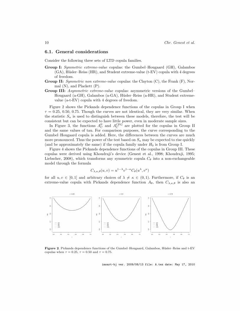
Figure 2 shows the Pickands dependence functions of the copulas in Group I whenτ = 0.25, 0.50, 0.75. Though the curves are not identical, they are very similar. Whenthe statistic Sn is used to distinguish between these models, therefore, the test will beconsistent but can be expected to have little power, even in moderate sample sizes.

In Figure 3, the functions APC and ACFG

C are plotted for the copulas in Group IIand the same values of tau. For comparison purposes, the curve corresponding to theGumbel–Hougaard copula is added. Here, the differences between the curves are muchmore pronounced. Thus the power of the test based on Sn may be expected to rise quickly(and be approximately the same) if the copula family under H0 is from Group I.

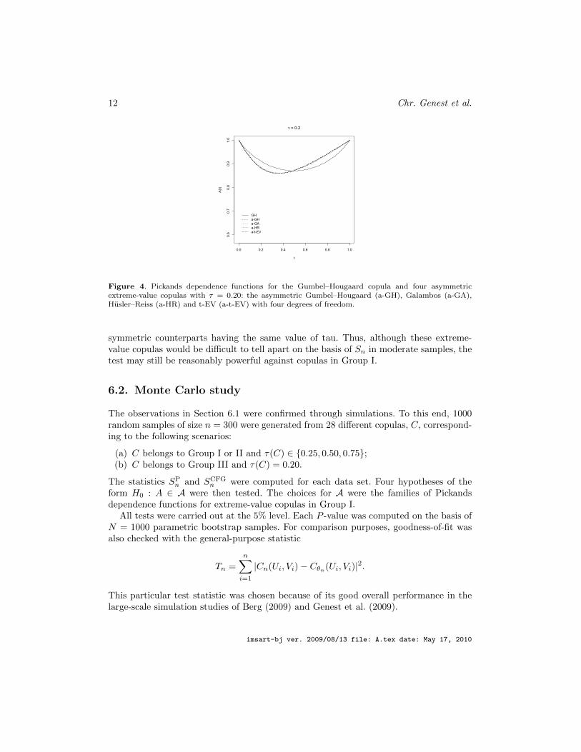
Figure 4 shows the Pickands dependence functions of the copulas in Group III. Thesecopulas were derived using Khoudraji’s device (Genest et al., 1998; Khoudraji, 1995;Liebscher, 2008), which transforms any symmetric copula Cθ into a non-exchangeablemodel through the formula

Cλ,κ,θ(u, v) = u1−λv1−κCθ(uλ, vκ)

for all u, v ∈ [0, 1] and arbitrary choices of λ 6= κ ∈ (0, 1). Furthermore, if Cθ is anextreme-value copula with Pickands dependence function Aθ, then Cλ,κ,θ is also an

0.0 0.2 0.4 0.6 0.8 1.0

0.6

0.7

0.8

0.9

1.0

! = 0.25

t

A(t)

GH

GA

HR

t-EV

0.0 0.2 0.4 0.6 0.8 1.0

0.6

0.7

0.8

0.9

1.0

! = 0.5

t

A(t)

GH

GA

HR

t-EV

0.0 0.2 0.4 0.6 0.8 1.0

0.6

0.7

0.8

0.9

1.0

! = 0.75

t

A(t)

GH

GA

HR

t-EV

Figure 2. Pickands dependence functions of the Gumbel–Hougaard, Galambos, Husler–Reiss and t-EVcopulas when τ = 0.25, τ = 0.50 and τ = 0.75.



0.0 0.2 0.4 0.6 0.8 1.0

0.5

0.6

0.7

0.8

0.9

1.0

! = 0.25

t

A-P(t)

GH

C

F

P

N

0.0 0.2 0.4 0.6 0.8 1.0

0.5

0.6

0.7

0.8

0.9

1.0

! = 0.5

t

A-P(t)

GH

C

F

P

N

0.0 0.2 0.4 0.6 0.8 1.0

0.5

0.6

0.7

0.8

0.9

1.0

! = 0.75

t

A-P(t)

GH

C

F

P

N

0.0 0.2 0.4 0.6 0.8 1.0

0.5

0.6

0.7

0.8

0.9

1.0

! = 0.25

t

A-CFG(t)

GH

C

F

P

N

0.0 0.2 0.4 0.6 0.8 1.0

0.5

0.6

0.7

0.8

0.9

1.0

! = 0.5

t

A-CFG(t)

GH

C

F

P

N

0.0 0.2 0.4 0.6 0.8 1.0

0.5

0.6

0.7

0.8

0.9

1.0

! = 0.75

t

A-CFG(t)

GH

C

F

P

N

Figure 3. Plots of APC (top) and ACFG

C (bottom) when C is the Gumbel–Hougaard (GH), Clayton (C),Frank (F), Normal (N) and Plackett (P) copulas with τ = 0.25 (left), τ = 0.50 (middle) and τ = 0.75(right).

extreme-value copula. Its Pickands dependence function is given at all t ∈ [0, 1] by

Aλ,κ,θ(t) = (1− κ)t+ (1− λ)(1− t) + {κt+ λ(1− t)}Aθ{

κt

κt+ λ(1− t)

}.

Note that the dependence in Cλ,κ,θ is limited. For, by the Frechet–Hoeffding inequality,

Cλ,κ,θ(u, v) ≤ u1−λv1−κ min(uλ, vκ) = min(uv1−κ, vu1−λ).

As the right-hand term is the Marshall–Olkin copula MOλ,κ, Example 5.5 of Nelsen(2006) implies that

τ(Cλ,κ,θ) ≤ τ(MOλ,κ) =κλ

κ+ λ− κλ.

In the present study, the values λ = 0.3, κ = 0.8 were used and hence τ(Cλ,κ,θ) couldnot exceed 0.279. For each choice of copula family Cθ in Group III, the parameter θ wasset to make Kendall’s tau equal to 0.20.

Figure 4 shows that the Pickands dependence functions of the copulas in Group IIIare very similar, though distinct. They are, however, easily distinguished from their



0.0 0.2 0.4 0.6 0.8 1.0

0.6

0.7

0.8

0.9

1.0

! = 0.2

t

A(t)

GH

a-GH

a-GA

a-HR

a-t-EV

Figure 4. Pickands dependence functions for the Gumbel–Hougaard copula and four asymmetricextreme-value copulas with τ = 0.20: the asymmetric Gumbel–Hougaard (a-GH), Galambos (a-GA),Husler–Reiss (a-HR) and t-EV (a-t-EV) with four degrees of freedom.

symmetric counterparts having the same value of tau. Thus, although these extreme-value copulas would be difficult to tell apart on the basis of Sn in moderate samples, thetest may still be reasonably powerful against copulas in Group I.

6.2. Monte Carlo study

The observations in Section 6.1 were confirmed through simulations. To this end, 1000random samples of size n = 300 were generated from 28 different copulas, C, correspond-ing to the following scenarios:

(a) C belongs to Group I or II and τ(C) ∈ {0.25, 0.50, 0.75};(b) C belongs to Group III and τ(C) = 0.20.

The statistics SPn and SCFG

n were computed for each data set. Four hypotheses of theform H0 : A ∈ A were then tested. The choices for A were the families of Pickandsdependence functions for extreme-value copulas in Group I.

All tests were carried out at the 5% level. Each P -value was computed on the basis ofN = 1000 parametric bootstrap samples. For comparison purposes, goodness-of-fit wasalso checked with the general-purpose statistic

Tn =

n∑i=1

|Cn(Ui, Vi)− Cθn(Ui, Vi)|2.

This particular test statistic was chosen because of its good overall performance in thelarge-scale simulation studies of Berg (2009) and Genest et al. (2009).



Table 1. Percentage of rejection of H0 for copulas in Group I when n = 300.

H0 True τ = 0.25 τ = 0.50 τ = 0.75Tn SP

n SCFGn Tn SP

n SCFGn Tn SP

n SCFGn

GH GH 4.2 3.8 4.0 4.0 4.8 3.6 4.2 5.3 5.5GA 4.8 4.3 4.2 4.4 3.8 3.8 4.8 4.3 4.3HR 4.8 4.2 4.0 5.4 3.4 3.9 3.7 3.1 1.7

t-EV 4.2 3.8 4.5 5.1 5.5 6.4 4.8 7.5 8.9

GA GH 4.5 4.7 3.9 4.0 5.8 4.7 4.4 5.6 6.8GA 4.3 4.6 4.0 5.5 3.9 4.8 4.3 4.7 4.6HR 4.6 4.8 4.2 5.0 3.4 3.4 3.7 3.7 1.8

t-EV 4.6 4.7 4.4 5.3 8.0 7.1 5.7 8.2 10.9

HR GH 4.6 6.4 4.4 4.3 9.6 7.5 4.5 9.6 15.7GA 4.3 5.4 4.5 5.1 6.6 7.2 5.1 8.4 11.7HR 4.9 5.2 4.2 5.3 4.3 3.9 4.0 4.3 3.3

t-EV 4.6 5.9 4.8 5.8 13.7 11.5 6.6 14.9 29.3

t-EV GH 4.2 3.4 4.0 4.1 3.9 2.9 4.0 3.3 2.4GA 4.1 4.3 4.4 4.8 3.4 3.9 4.6 3.0 1.7HR 4.7 4.1 4.4 5.4 3.2 3.4 3.8 2.2 1.3

t-EV 4.6 3.7 4.2 4.7 4.8 5.2 4.1 4.3 4.7

Tables 1–4 report the percentage of rejection of the four null hypotheses under eachscenario. Though this made little difference, these results are for the endpoint-correctedversions of AP

n and ACFGn , defined for all t ∈ [0, 1] by

1/APn,c(t) = 1/AP

n(t)− (1− t){1/APn(0)− 1} − t{1/AP

n(1)− 1}

andlogACFG

n,c (t) = log{ACFGn (t)} − (1− t) log{ACFG

n (0)} − t log{ACFGn (1)}.

Before commenting the results, note that for copulas in Groups I and II, the real-valued dependence parameter of each data set was estimated by inversion of Kendall’stau; its implementation relied on the numerical approximation technique of Kojadinovicand Yan (2010a). For copulas in Group III, which involve several parameters, maximumpseudo-likelihood estimation was used (Genest et al., 1995; Shih and Louis, 1995).

6.3. Results

It is clear from Table 1 that when n = 300, the tests based on Tn, SPn and SCFG

n cannotdistinguish between copulas in Group I. When τ = 0.25, all rejection rates are withinsampling error from the nominal level. There are only small signs of improvement as τrises to 0.50 and 0.75. The best scores are obtained when testing for the Husler–Reissmodel with SCFG

n when τ = 0.75. Globally there is little to choose between the tests.Table 2 shows what happens when n = 1000. Power is on the rise, especially when τ =

0.75. In the latter case, it seems preferable to base the test on SCFGn rather than on SP

n ;



Table 2. Percentage of rejection of H0 for copulas in Group I when n = 1000.

H0 True τ = 0.25 τ = 0.50 τ = 0.75Tn SP

n SCFGn Tn SP

n SCFGn Tn SP

n SCFGn

GH GH 4.9 4.7 5.3 4.0 5.9 6.0 3.8 5.2 5.4GA 5.1 5.8 4.0 5.9 4.4 5.1 4.8 3.8 4.2HR 5.1 6.3 6.3 5.1 6.3 9.0 3.4 3.5 9.2

t-EV 5.4 4.4 5.4 6.1 6.2 6.9 5.4 9.8 15.9

GA GH 5.2 7.4 6.1 4.4 8.1 8.4 4.3 5.6 7.3GA 5.0 5.6 4.0 5.4 5.1 5.4 4.8 4.4 5.2HR 4.4 5.0 5.2 4.5 4.5 6.2 3.5 3.1 6.2

t-EV 6.1 6.9 6.6 6.7 9.4 12.7 5.5 12.8 23.1

HR GH 6.2 10.6 8.6 5.1 17.6 17.8 5.5 18.1 40.2GA 5.4 6.6 4.1 5.6 8.1 8.8 5.5 12.7 23.4HR 4.6 5.9 5.5 4.2 4.9 5.1 3.4 4.7 5.6

t-EV 6.6 10.1 8.2 8.2 27.0 34.4 6.5 45.2 81.7

t-EV GH 4.7 4.7 5.3 4.4 4.4 5.7 4.0 3.4 3.0GA 4.8 5.6 4.2 5.6 4.8 6.0 4.8 3.0 3.7HR 5.3 6.4 6.1 5.5 8.5 12.3 4.3 3.9 28.7

t-EV 5.1 4.5 5.5 5.6 4.8 5.3 5.2 4.5 4.7

they both do better than the test based on Tn. Overall, the results remain disappointinglylow, except when testing for the Husler–Reiss model with τ ≥ 0.50.

These observations are in line with Figure 2, which shows striking similarities betweenthe Gumbel–Hougaard, Galambos, Husler–Reiss and t-EV copula with 4 degrees of free-dom. While SP

n and SCFGn still have trouble telling them apart when the sample size is

1000, their power eventually rises when n → ∞, as explained in Section 5. To illustratethis point, samples of various sizes were generated from the Gumbel–Hougaard copulawith τ = 0.50 and the statistic SCFG

n was used to test for the Galambos family. Thefollowing results, based on 1000 repetitions and N = 1000 bootstrap samples, give anidea of the sample sizes needed to differentiate models in Group I:

Sample size n 5,000 10,000 20,000 40,000Percentage of rejection of H0 10.8 22.6 60.2 97.3

Returning to the case n = 300, one can see from Table 3 that the test based on SCFGn

is quite good at detecting non extreme-value LTD alternatives from Group II. Its poweris higher than those of SP

n and Tn, except when the data are generated from the Claytonor the Normal copula with τ = 0.25. Interestingly, the general-purpose test based on Tnis often second best. The statistic SP

n has the edge only for the Clayton when τ = 0.25;it does very poorly against the Frank, and against the Normal when τ = 0.75.

These results are in close agreement with the plots displayed in Figure 3. Consider forinstance the case where SP

n is used to test for the Gumbel–Hougaard copula from weaklydependent data (τ = 0.25). From Table 3, the alternatives can be ranked as follows indecreasing order of power:



Table 3. Percentage of rejection of H0 for copulas in Group II when n = 300.

H0 True τ = 0.25 τ = 0.50 τ = 0.75Tn SP

n SCFGn Tn SP

n SCFGn Tn SP

n SCFGn

GH C 98.8 99.5 82.1 100.0 100.0 100.0 100.0 100.0 100.0F 36.6 11.0 48.0 82.0 7.1 100.0 92.1 27.2 100.0N 26.9 21.9 21.8 43.5 44.9 66.9 37.5 18.7 82.3P 34.3 17.3 43.4 68.0 44.6 98.6 65.0 71.6 100.0

GA C 98.9 99.7 84.0 100.0 100.0 100.0 100.0 100.0 100.0F 39.8 15.1 50.1 83.4 10.2 100.0 92.1 29.9 100.0N 28.1 25.7 21.9 44.0 49.0 69.5 37.4 21.5 83.2P 37.7 23.4 45.0 70.8 57.1 99.0 65.7 76.7 100.0

HR C 99.1 99.9 84.5 100.0 100.0 100.0 100.0 100.0 100.0F 42.3 18.8 52.5 85.2 18.9 100.0 93.7 42.1 100.0N 28.3 29.0 22.5 46.0 55.7 73.3 38.9 34.8 89.8P 41.1 28.8 48.3 75.1 74.5 99.5 73.1 92.1 100.0

t-EV C 98.6 99.5 82.6 100.0 100.0 100.0 100.0 100.0 100.0F 36.7 11.1 48.3 81.3 5.0 100.0 90.9 18.9 100.0N 26.5 21.8 21.7 43.5 42.7 66.2 36.9 10.6 74.2P 34.8 17.2 43.7 67.7 35.7 98.1 62.1 53.2 99.8

Table 4. Percentage of rejection of H0 for copulas in Group III when n = 300.

H0 True Tn SPn SCFG

n

GH a-GH 32.7 40.9 86.5a-GA 33.5 42.8 86.7a-HR 28.4 37.5 83.5a-t-EV 33.1 41.4 88.6

GA a-GH 33.4 40.8 89.2a-GA 34.0 42.3 89.3a-HR 28.4 38.1 86.5a-t-EV 32.7 40.6 90.5

H0 True Tn SPn SCFG

n

HR a-GH 36.2 37.5 93.3a-GA 31.7 39.1 89.7a-HR 32.6 40.9 90.3a-t-EV 40.5 42.8 92.3

t-EV a-GH 32.0 41.2 87.1a-GA 33.2 43.3 87.8a-HR 27.3 38.4 83.6a-t-EV 31.3 40.7 88.7

Clayton � Normal � Plackett � Frank.

Looking at Figure 3, one finds that this ordering is concordant with the overall degree ofdissimilarity between AP

C and A. In this case as in others, it is found that at fixed samplesize, curves that look alike are harder to distinguish than others.

Finally, Table 4 shows that the statistic SCFGn is much better than the other two at

detecting asymmetric extreme-value alternatives. The overall good performance of thistest is consistent with evidence from Genest and Segers (2009) that ACFG

n is generallya better nonparametric estimator of the Pickands dependence function than AP

n . Whenthe margins are known, this phenomenon is well documented; see, e.g., Caperaa et al.(1997), Hall and Tajvidi (2000) or Rojo-Jimenez et al. (2001).



Table 5. Values of the statistics SPn , SCFG

n and approximate P -values computed using N = 2500parametric bootstrap samples for the insurance data.

Model SPn P -value SCFG

n P -value

GH 0.087 0.073 0.048 0.171GA 0.084 0.074 0.045 0.184HR 0.088 0.067 0.049 0.157t-EV 0.088 0.069 0.048 0.166a-GH 0.052 0.274 0.012 0.152a-GA 0.046 0.325 0.009 0.244a-HR 0.051 0.272 0.011 0.174a-t-EV 0.062 0.204 0.015 0.122

7. Conclusion

Copula models are now common. As illustrated, e.g., by Ben Ghorbal et al. (2009), so aresituations in which the dependence structure of a random pair (X,Y ) is well representedby an extreme-value copula, even though X and Y themselves do not necessarily exhibitextreme-value behavior. In such cases, the statistics considered here can be used to testthe goodness-of-fit of specific parametric copula families of the form (2), such as theGumbel–Hougaard, Galambos, Husler–Reiss or Student extreme-value copula.

Theoretical and empirical evidence presented here shows that the nonparametric testsbased on the Cramer–von Mises statistic Sn are generally consistent and that they arean effective tool for distinguishing between symmetric and asymmetric extreme-valuecopulas, as well as for detecting other left-tail decreasing (LTD) dependence structures.

Except in the presence of massive data, however, it seems very difficult to discriminatebetween extreme-value copulas whose Pickands dependence functions are close. This maycome as somewhat of a disappointment but upon reflection one may wonder whether inthe light of Figure 2, there is any practical difference, say, between the Gumbel–Hougaardand the Galambos copula when they have the same value of Kendall’s tau.

For example, many studies have concluded that a Gumbel–Hougaard copula structureis adequate for the insurance data mentioned in the Introduction; see, e.g., Frees andValdez (1998), Genest et al. (1998), Chen and Fan (2005), Denuit et al. (2006), Dupuisand Jones (2006), Genest et al. (2006) or Kojadinovic and Yan (2010b). In these papers,comparisons were made between the Gumbel–Hougaard model and non extreme-valuecopulas that were either Archimedean or meta-elliptical.

As Ben Ghorbal et al. (2009) conclude that the data exhibit extreme-value dependence,it may be worth comparing the Gumbel–Hougaard structure with other extreme-valuecopulas from Groups I and III. This is done in Table 5 using the statistics SP

n and SCFGn

and the inversion of Kendall’s tau to estimate θ. Because the test is yet to be adapted tothe case of censoring, the analysis ignored the 34 claims for which the policy limit wasreached. Each P -value in the table is based on N = 2500 bootstrap samples. Given thecomparatively small sample size, n = 1466, it does not come as a surprise that no model



Figure 5. Nonparametric estimates APn,c and ACFG

n,c , and fitted Pickands dependence function for theGalambos copula (left) and for the asymmetric Galambos copula (right).

is rejected at the 5% level.Figure 5 displays the endpoint-corrected estimates AP

n,c and ACFGn,c for the data at hand.

For comparison, the best-fitting symmetric and asymmetric Galambos extreme-valuecopula are superimposed. Although these two models yield the highest P -values, theyare not significantly better than the alternatives listed in Table 5. Given the estimators’sampling variability, the data set is simply too small to distinguish between them. Thisis not a major concern, however, as predictions derived from these various models wouldbe roughly the same. To paraphrase Box and Draper (1987, p. 424), it may be that allthese models are false, but they are nearly equivalent and probably equally useful.

Appendix A: Proof of Proposition 1

Let An denote either APn or ACFG

n , and write An,θn = An−Bn,θ0 , where Bn,θ0 =√n (Aθn−

Aθ0). As the sequence Θn is assumed to converge weakly, it is tight. Thus, for given δ > 0,there exists L = L(δ) such that Pr (‖Θn‖ > L) < δ holds for every integer n. Therefore,for given ζ > 0,

Pr

{supt∈[0,1]

|Bn,θ0(t)− A>θ0(t)Θn| > ζ

}≤

Pr

{supt∈[0,1]

|Bn,θ0(t)− A>θ0(t)Θn| > ζ, ‖Θn‖ ≤ L

}+ Pr (‖Θn‖ > L) ≤

Pr

{supt∈[0,1]

|Bn,θ0(t)− A>θ0(t)Θn| > ζ, ‖Θn‖ ≤ L

}+ δ.

An application of the Mean Value Theorem then implies that for every realizationω of the process and every t ∈ [0, 1], Bn,θ0(t, ω) = A>Θ∗

n(t,ω)(t)Θn(ω), where Θ∗n(t, ω) =



θ0 + ε(t, ω)n−1/2Θn(ω) for some ε(t, ω) ∈ [0, 1]. It then follows from Condition (6) that

limn→∞

Pr

{supt∈[0,1]

|Bn,θ0(t)− A>θ0(t)Θn| > ζ, ‖Θn‖ ≤ L

}≤

limn→∞

Pr

{‖Θn‖ sup

t∈[0,1]

|AΘ∗n(t)(t)− Aθ0(t)| > ζ, ‖Θn‖ ≤ L

}≤

limn→∞

Pr

{sup

‖θ−θ0‖≤n−1/2L

supt∈[0,1]

|Aθ(t)− Aθ0(t)| > ζ/L

}= 0.

This completes the argument.

Appendix B: Validity of the parametric bootstrap

To avoid repetitions, let An denote either APn or ACFG

n , and let A stand for either AP orACFG. The following conditions, adapted from Genest and Remillard (2008), ensure thevalidity of the parametric bootstrap for computing P -values for the proposed tests.

(a) The family {Cθ : θ ∈ O} of extreme-value copulas must be such that:

(i) The parameter space O is an open subset of Rp.(ii) Members of the family are identifiable, i.e., for every ε > 0,

inf

{supt∈[0,1]

‖Aθ(t)−Aθ0(t)‖ : θ ∈ O and ‖θ − θ0‖ > ε

}> 0.

(iii) The mapping θ 7→ Aθ is Frechet differentiable with derivative θ 7→ Aθ, i.e., forall θ0 ∈ O,

lim‖h‖↓0

supt∈[0,1]

‖Aθ0+h(t)−Aθ0(t)− A>θ0(t)h‖‖h‖

= 0.

(iv) Cθ has a Lebesgue density cθ for all θ ∈ O.

(v) The density cθ admits first and second order derivatives with respect to allcomponents of θ ∈ O. The gradient (row) vector with respect to θ is denotedcθ and the Hessian matrix cθ.

(vi) For arbitrary (u, v) ∈ (0, 1)2 and every θ0 ∈ O, θ 7→ cθ(u, v)/cθ(u, v) andθ 7→ cθ(u, v)/cθ(u, v) are continuous at θ0, Cθ0 almost surely.

(vii) For every θ0 ∈ O, there exist a neighborhood N of θ0 and a Lebesgue-integrable function h : (0, 1)2 → R such that supθ∈N ‖cθ(u, v)‖ ≤ h(u, v)holds for all (u, v) ∈ (0, 1)2.



(viii) For every θ0 ∈ O, there exist a neighborhood N of θ0 and Cθ0-integrablefunctions h1, h2 : (0, 1)2 → R such that for all (u, v) ∈ (0, 1)2,

supθ∈N

∥∥∥∥ cθ(u, v)

cθ(u, v)

∥∥∥∥2

≤ h1(u, v) and supθ∈N

∥∥∥∥ cθ(u, v)

cθ(u, v)

∥∥∥∥ ≤ h2(u, v).

(b) In addition, the estimators An and θn satisfy the following:

(i) (An,Θn,Wn) (A,Θ,W) in D([0, 1],R) × Rp⊗2 as n → ∞, where the limitis a centered Gaussian process. Here,

Wn = n−1/2n∑i=1

c>θ0(U∗i , V∗i )

cθ0(U∗i , V∗i )

for a random sample (U∗1 , V∗1 ), . . . , (U∗n, V

∗n ) from Cθ0 and W isN (0, IP ), where

IP is the Fisher information matrix; see Genest and Remillard (2008, p. 1101).

(ii) Eθ0(ΘW>) = J , where J is the p× p identity matrix. Further, Eθ0{A(t)W} =Aθ0(t) for every t ∈ (0, 1).

Condition (b) can be checked as follows, under the assumption that (An,Θn) (A,Θ)as n → ∞. First, results from Chapter 5 of Ganßler and Stute (1987) can be combinedwith the Functional Delta Method (see, e.g., van der Vaart and Wellner, 1996, Section3.9) to see that as n→∞, (An,Θn,Cn,Wn) (A,Θ,C,W).

Next, observe that Eθ0{C(u, v)W} = Cθ0(u, v) for all u, v ∈ [0, 1], as per Genest andRemillard (2008, p. 1108). Given that for all t ∈ [0, 1],

AP(t) = −A2θ0(t)

∫ 1

0

Cθ0(x1−t, xt)dx

x

and

ACFG(t) = Aθ0(t)

∫ 1

0

Cθ0(x1−t, xt)dx

x log(x),

one can see that

Eθ0{AP(t)W} = −A2θ0(t)

∫ 1

0

Cθ0(x1−t, xt)dx

x

and

Eθ0{ACFG(t)W} = Aθ0(t)

∫ 1

0

Cθ0(x1−t, xt)dx

x log(x).

Interchanging the order of differentiation and integration, one gets Eθ0{AP(t)W} =Eθ0{ACFG(t)W} = Aθ0(t) for all t ∈ (0, 1).

As for the condition Eθ0(ΘW) = J , it can be verified using Proposition 4 of Genestand Remillard (2008) for the estimators based on maximum pseudo-likelihood and onthe inversion of Spearman’s rho. To handle the estimator based on Kendall’s tau, theirProposition 5 must be used instead.



Appendix C: Proof of Proposition 2

The proof closely mimics the argument presented in Appendix B of Genest and Segers(2009). To avoid duplication, the same notation is used and only the critical differencesare highlighted. This also offers an opportunity to correct minor typos in the originalsource.

First consider the process given by BPn(t) = n1/2

{1/AP

n(t)− 1/APC(t)

}for all t ∈ [0, 1]

and show that BPn B = −AP

C/(APC)2 as n→∞. Then

√n (AP

n −APC) =

−(APC)2BP

n

1 + n−1/2BPnA

PC

APC ,

as a consequence of the functional version of Slutsky’s lemma.Put kn = 2 log(n+ 1) and write

BPn(t) =

∫ 1

0

Cn(x1−t, xt)dx

x=

∫ ∞0

Cn(e−s(1−t), e−st) ds = I1,n + I2,n,

where for each t ∈ [0, 1],

I1,n(t) =

∫ ∞kn

Cn(e−s(1−t), e−st) ds, I2,n(t) =

∫ kn

0

Cn(e−s(1−t), e−st) ds.

The contribution of I1,n(t) is asymptotically negligible because the fact that s > knimplies min(e−s(1−t), e−st) < 1/(n+ 1) and hence

|Cn(e−s(1−t), e−st)| = n1/2C(e−s(1−t), e−st) ≤ n1/2 min(e−s(1−t), e−st) ≤ n1/2e−s/2.

Thus for all t ∈ [0, 1],

|I1,n(t)| ≤ n1/2

∫ ∞kn

C(e−s(1−t), e−st) ds ≤ n1/2

∫ ∞kn

e−s/2 ds ≤ 2

n1/2. (A1)

Consequently, the asymptotic behavior of BPn is determined entirely by I2,n. Invoking

the Stute representation given by Genest and Segers (2009), one may write I2,n = J1,n+J2,n + J3,n + o(1), where for each t ∈ [0, 1],

J1,n(t) =

∫ kn

0

αn(e−s(1−t), e−st) ds,

J2,n(t) = −∫ kn

0

αn(e−s(1−t), 1)C1(e−s(1−t), e−st) ds,

J3,n(t) = −∫ kn

0

αn(1, e−st)C2(e−s(1−t), e−st) ds.

Here, C1(u, v) = ∂C(u, v)/∂u, C2(u, v) = ∂C(u, v)/∂v, and αn is the empirical processassociated with the pairs (F (X1), G(Y1)), . . . , (F (Xn), G(Yn)).



Fix ω ∈ (0, 1/2) and write qω(t) = tω(1− t)ω for all t ∈ [0, 1]. Let also

K1(s, t) = qω{min(e−s(1−t), e−st)},K2(s, t) = qω(e−s(1−t)) C1(e−s(1−t), e−st),

K3(s, t) = qω(e−st) C2(e−s(1−t), e−st),

for all s ∈ (0,∞) and t ∈ [0, 1]. The proof that J1,n + J2,n + J3,n has the stated limitthen proceeds exactly as in Appendix B of Genest and Segers (2009), provided that fori = 1, 2, 3, there exists an integrable function K∗i : (0,∞)→ R such that Ki(s, t) ≤ K∗i (s)for all s ∈ (0,∞) and t ∈ [0, 1].

For K1, this is immediate because K1(s, t) ≤ e−ωs/2 for all s ∈ (0,∞) and t ∈ [0, 1].For K2, the facts that C is LTD and smaller than the Frechet–Hoeffding upper boundimply that

C1(e−s(1−t), e−st) ≤ es(1−t)C(e−s(1−t), e−st) ≤ es(1−t) min(e−s(1−t), e−st).

Now set m(t) = max(t, 1 − t) and note that qω(e−s(1−t)) ≤ e−ωs(1−t) for all s ∈ (0,∞)and t ∈ [0, 1]. Therefore,

K2(s, t) ≤ es(1−ω)(1−t)e−sm(t) ≤ es(1−ω)m(t)e−sm(t) = e−sωm(t) ≤ e−ωs/2

because m(t) ≥ 1/2 for all t ∈ [0, 1]. The argument for K3 is similar.

Turning to the ACFGn estimator, observe that

BCFGn (t) = n1/2{logACFG

n (t)− logACFGC (t)}

=

∫ 1

0

Cn(x1−t, xt)dx

x log(x)= −

∫ ∞0

Cn(e−s(1−t), e−st)ds

s

for all t ∈ [0, 1]. This process can be written as −(I1,n + I2,n + I3,n), where

I1,n(t) =

∫ ∞kn


s,

I2,n(t) =

∫ kn

`n


s,

I3,n(t) =

∫ `n

0


s,

with kn = 2 log(n+ 1) as above and `n = 1/(n+ 1).Arguing as in (A1), one sees that |I1,n| ≤ n−1/2. Similarly, I3,n is negligible asymp-

totically. For, if s ∈ (0, `n) and t ∈ [0, 1], one has

min(e−s(1−t), e−st) ≥ e−1/(n+1) >n

n+ 1



and hence Cn(e−s(1−t), e−st) = 1. Furthermore, the fact that C is LTD implies thatC(e−s(1−t), e−st) ≥ e−s for all s ∈ (0,∞) and t ∈ [0, 1]. Therefore,

|Cn(e−s(1−t), e−st)| ≤ n1/2(1− e−s) ≤ n1/2s.

Therefore, |I3,n| ≤ n1/2`n ≤ n−1/2. As a result, the asymptotic behavior of BCFGn is

determined entirely by I2,n. Following Genest and Segers (2009), one can further writeI2,n = J1,n + J2,n + J3,n + o(1), where for all t ∈ [0, 1],

J1,n(t) =

∫ kn

`n

αn(e−s(1−t), e−st)ds

s,

J2,n(t) = −∫ kn

`n

αn(e−s(1−t), 1)C1(e−s(1−t), e−st)ds

s,

J3,n(t) = −∫ kn

`n

αn(1, e−st)C2(e−s(1−t), e−st)ds

s.

The joint asymptotic behavior of these terms can be determined in the same way asbefore. The only difference is that the integration measure is now ds/s. For s ∈ [1,∞),the same upper bounds K∗1 , K∗2 , K∗3 apply, and they have already been shown to beintegrable on this domain. To obtain an integrable bound for K1 on (0, 1), it suffices touse the fact that K1(s, t) ≤ (1− e−sm(t))ω ≤ {sm(t)}ω ≤ sω. The same bound works forboth K2 and K3 because Ci ∈ [0, 1] for i = 1, 2. This completes the argument.

Acknowledgments

Grants in support of this work were provided by the Natural Sciences and EngineeringResearch Council of Canada, the Fonds quebecois de la recherche sur la nature et lestechnologies, and the Institut de finance mathematique de Montreal.

References

Ben Ghorbal, N., Genest, C., Neslehova, J., 2009. On the Ghoudi, Khoudraji, and Rivesttest for extreme-value dependence. The Canadian Journal of Statistics 37, 534–552.

Berg, D., 2009. Copula goodness-of-fit testing: An overview and power comparison. TheEuropean Journal of Finance 15, 675–701.

Box, G. E. P., Draper, N. R., 1987. Empirical Model-Building and Response Surfaces.Wiley, New York.

Caperaa, P., Fougeres, A.-L., Genest, C., 1997. A nonparametric estimation procedurefor bivariate extreme value copulas. Biometrika 84, 567–577.

Chen, X., Fan, Y., 2005. Pseudo-likelihood ratio tests for semiparametric multivariatecopula model selection. The Canadian Journal of Statistics 33, 389–414.



Cherubini, U., Luciano, E., Vecchiato, W., 2004. Copula Methods in Finance. Wiley, NewYork.

Denuit, M., Dhaene, J., Goovaerts, M. J., Kaas, R., 2005. Actuarial Theory for DependentRisk: Measures, Orders and Models. Wiley, New York.

Denuit, M., Purcaru, O., Van Keilegom, I., 2006. Bivariate Archimedean copula modellingfor censored data in nonlife assurance. Journal of Actuarial Practice 13, 5–32.

Dupuis, D. J., Jones, B. L., 2006. Multivariate extreme value theory and its usefulnessin understanding risk. North American Actuarial Journal 10, 1–27.

Falk, M., Reiss, R.-D., 2005. On Pickands coordinates in arbitrary dimensions. Journalof Multivariate Analysis 92, 426–453.

Frees, E. W., Valdez, E. A., 1998. Understanding relationships using copulas. NorthAmerican Actuarial Journal 2, 1–25.

Ganßler, P., Stute, W., 1987. Seminar on Empirical Processes. DMV Seminar 9.Birkhauser, Basel, Switzerland.

Garralda-Guillem, A. I., 2000. Structure de dependance des lois de valeurs extremesbivariees. Comptes rendus de l’Academie des sciences de Paris, Serie I Mathematique330, 593–596.

Genest, C., Ghoudi, K., Rivest, L.-P., 1995. A semiparametric estimation procedure ofdependence parameters in multivariate families of distributions. Biometrika 82, 543–552.

Genest, C., Ghoudi, K., Rivest, L.-P., 1998. Discussion of “Understanding relationshipsusing copulas,” by E. W. Frees and E. A. Valdez. North American Actuarial Journal2, 143–149.

Genest, C., Quessy, J.-F., Remillard, B., 2006. Goodness-of-fit procedures for copulasmodels based on the probability integral transformation. Scandinavian Journal ofStatistics 33, 337–366.

Genest, C., Remillard, B., 2008. Validity of the parametric bootstrap for goodness-of-fittesting in semiparametric models. Annales de l’Institut Henri Poincare: Probabiliteset Statistiques 44, 1096–1127.

Genest, C., Remillard, B., Beaudoin, D., 2009. Goodness-of-fit tests for copulas: A reviewand a power study. Insurance: Mathematics and Economics 44, 199–213.

Genest, C., Segers, J., 2009. Rank-based inference for bivariate extreme-value copulas.The Annals of Statistics 37, 2990–3022.

Ghoudi, K., Khoudraji, A., Rivest, L.-P., 1998. Proprietes statistiques des copules devaleurs extremes bidimensionnelles. The Canadian Journal of Statistics 26, 187–197.

Gudendorf, G., Segers, J., 2009. Nonparametric estimation of an extreme-value copulain arbitrary dimensions. preprintArXiv:0910.0845v1.

Hall, P., Tajvidi, N., 2000. Distribution and dependence-function estimation for bivariateextreme-value distributions. Bernoulli 6, 835–844.

Khoudraji, A., 1995. Contributions a l’etude des copules et a la modelisation des valeursextremes bivariees. Ph.D. thesis, Universite Laval, Quebec, Canada.

Kim, G., Silvapulle, M. J., Silvapulle, P., 2007. Comparison of semiparametric and para-metric methods for estimating copulas. Computational Statistics and Data Analysis51, 2836–2850.



Klugman, S. A., Parsa, R., 1999. Fitting bivariate loss distributions with copulas. Insur-ance: Mathematics and Economics 24, 139–148.

Kojadinovic, I., Yan, J., 2010a. Comparison of three semiparametric methods for estimat-ing dependence parameters in copula models. Insurance: Mathematics and Economics47, in press.

Kojadinovic, I., Yan, J., 2010b. Modeling multivariate distributions with continuous mar-gins using the copula R package. Journal of Statistical Software, in press.

Liebscher, E., 2008. Construction of asymmetric multivariate copulas. Journal of Multi-variate Analysis 99, 2234–2250.

McNeil, A. J., Frey, R., Embrechts, P., 2005. Quantitative Risk Management: Concepts,Techniques, and Tools. Princeton University Press, Princeton, NJ.

Nelsen, R. B., 2006. An Introduction to Copulas, Second Edition. Springer, New York.Pickands, III, J., 1981. Multivariate extreme value distributions. In: Proceedings of the

43rd Session of the International Statistical Institute, Vol. 2 (Buenos Aires, 1981).Vol. 49. pp. 859–878, 894–902, with a discussion.

Rojo-Jimenez, J., Villa-Diharce, E., Flores, M., 2001. Nonparametric estimation of thedependence function in bivariate extreme value distributions. Journal of MultivariateAnalysis 76, 159–191.

Ruschendorf, L., 1976. Asymptotic distributions of multivariate rank order statistics. TheAnnals of Statistics 4, 912–923.

Salvadori, G., De Michele, C., Kottegoda, N. T., Rosso, R., 2007. Extremes in Nature:An Approach Using Copulas. Springer, New York.

Shih, J. H., Louis, T. A., 1995. Inferences on the association parameter in copula modelsfor bivariate survival data. Biometrics 51, 1384–1399.

Sklar, A., 1959. Fonctions de repartition a n dimensions et leurs marges. Publications del’Institut de statistique de l’Universite de Paris 8, 229–231.

van der Vaart, A. W., Wellner, J. A., 1996. Weak Convergence and Empirical Processes.Springer, New York.

Yan, J., Kojadinovic, I., 2009. Copula: Multivariate Dependence with Copulas. R PackageVersion 0.8–12.

Zhang, D., Wells, M. T., Peng, L., 2008. Nonparametric estimation of the dependencefunction for a multivariate extreme value distribution. Journal of Multivariate Analysis99, 577–588.

Received August 2009 and revised January 2010


Date post:	20-May-2018
Category:	Documents
Upload:	lekhanh
View:	215 times
Download:	1 times

A goodness-of- t test for bivariate extreme-value...

Documents