A GRAPH-THEORETIC ANALYSIS OF CHEMICAL REACTION NETWORKS I. Invariants, Network Equivalence and Nonexistence of Various Types of Steady States ∗ Hans G. Othmer Department of Mathematics University of Utah Salt Lake City, Utah 84112 1981 * Based on Rutgers University Course Notes, 1979 1
Transcript
A GRAPH-THEORETIC ANALYSIS OF
CHEMICAL REACTION NETWORKS
I. Invariants, Network Equivalence and Nonexistence of
Various Types of Steady States∗
Hans G. OthmerDepartment of Mathematics
University of UtahSalt Lake City, Utah 84112
1981
∗Based on Rutgers University Course Notes, 1979
1
Contents
1 Abstract 2
2 Introduction 2
3 How Stoichiometry and Network Structure are Reflected in the Dynamical Equations. 43.1 The Graph Associated with a Reaction Network . . . . . . . . . .. . . . . . . . . . . . . . . . . . . 43.2 Some Basic Concepts from Graph Theory and Convex Analysis. . . . . . . . . . . . . . . . . . . . . 7
6 Necessary Conditions for the Existence of a Steady State. 246.1 The Relationship Between Local and Global Deficiency. . .. . . . . . . . . . . . . . . . . . . . . . 246.2 Nonexistence of Balanced Flows . . . . . . . . . . . . . . . . . . . . .. . . . . . . . . . . . . . . . 276.3 Conditions under whichS2 = φ. . . . . . . . . . . . . . . . . . . . . . . . . . . . . . . . . . . . . . 296.4 A Flow Chart For Determining Whether Any Steady State CanExist. . . . . . . . . . . . . . . . . . . 32
7 Discussion 32
References 35
1 Abstract
The dynamical behavior of a chemically-reacting system is determined by the stoichiometry of the reactions, thestructure of the graph underlying the network, and the reaction phenomenology embodied in the rate laws. Herein wedevelop a new approach to the analysis of networks, using graph-theoretic techniques, that separates the individualinfluences to the extent possible, and facilitates the analysis of their interaction. We show how the reaction invariantsare related to the stoichiometry and the network structure and give sufficient conditions under which the reactionsimplex is not compact. The notion of dynamical equivalenceof networks is defined and three types of equivalencetransformations are introduced. In particular, it is shownthat a network of positive deficiency, a term defined later, isdynamically equivalent to one with zero deficiency. In our approach, the steady states of any network fall into threeclasses, and conditions are given under which each of these classes is empty.
2 Introduction
The objective in a qualitative analysis of a dynamical system described by an evolution equation of the formu =
F (u, p), whereu is the state andp is a parameter vector, is to predict the qualitative evolution ofu for different initialconditions, and to determine how the evolution depends on the parameters. The basic problem is the same, irrespectiveof whether the equation arises from a problem in chemical reaction dynamics, ecological interactions between species,membrane transport or a variety of similar problems. However, the constraints inherent in a particular problem, such asthe non-negativity ofu or of some of the parameters, may place additional constraints on the structure of the equations,
2
and such constraints may make the general analysis of wide class of problems feasible. This is particularly true forproblems of the sort mentioned, for in these the pattern of ’reaction’ between the various species imposes a great dealof structure on the governing equations. Our objective hereis to develop a general graph-theoretic approach to theanalysis of the equations that describe open reacting systems, an approach that makes systematic use of the structuredictated by the reactions. The general ideas can be applied to a variety of other problems, as examples in sequels tothis paper will show.
Two fundamental properties of closed reacting systems are crucial to the analysis of their equilibrium and dynamicbehavior. Firstly, the fact that the mass of the mixture is constant implies that the reaction simplex, a term definedlater, is compact, and therefore all closed systems have a least one equilibrium point. Secondly, the hypothesis that thedissipation is non-negative and vanishes only when the net rate of all reactions vanish implies that all trajectories thatbegin in the interior of the simplex approach an equilibriumpoint ast → ∞. In an open system, which by definitioncan exchange material with its environment, reaction invariants such as the total mass need not be time-independentand there is noa priori guarantee that a steady state exists. Even if one does exist,the dissipation is generally notminimized at the steady state, as the following argument shows.
Suppose that a system is spatially uniform and that its dynamics are described by the solution of
dc
dt= J(c, co) + νR(c),
whereJ(c, co) is the exchange flux between the system and a time-invariant bath,ν is the usual stoichiometric matrix(Aris 1965) andRi(c) is the intrinsic rate of the ith reaction. The free energy perunit volume of the system isG =< µ, c >, whereµ is the chemical potential vector,1 and its rate of change along trajectories of the system is givenby
The first term represents the free energy flux into the system andΦ is the internal dissipation due both to reaction andtransport. At a steady state the flux balances the dissipation, but there is noa priori reason why eitherG or Φ shouldhave a local minimum at a steady state. As Denbigh (1952) firstpointed out, it would be fortuitous if the solution ofthe system
∂Φ
∂ci
= 0 i = 1, . . . n
coincided with the solution of
0 = J(c, co) + νR(c).
It happens that they do coincide when the rate expressions are linear functions of the affinities, the phenomenologicalcoefficients are constant, and the Onsager relations are satisfied (DeGroot and Mazur 1962). In this case it is easyto show thatdΦ/dt ≤ 0. However, this so-called ’evolution criterion’ generallyfails even in a closed system, as anexample in Othmer (1981) shows. There are Lyapunov functions for certain classes of open system (see the Discussionsection), but in general there is no universal evolution criterion for open system comparable to ’dG/dt ≤ 0’ for closedsystems, as Mel and Ewald (1974) have shown. Thus the analysis of open systems necessarily proceeds on more of acase-by-case basis, but it is desirable to identify generalclasses of mechanisms for which the dynamical behavior canreadily be determined. The exchange fluxJ(c, co) can formally be viewed as the result of a reactionM0
M that’converts’ a species at one concentration to the same species at a different concentration, and from this viewpoint, thedifferent modes of transport, such as convection in a CSTR orfacilitated transport across a membrane, differ primarily
1Here and hereafter<, > denotes the Euclidean inner product onRn.
3
in the ’mechanism’ of the exchange reaction. We shall adopt this viewpoint here and use the word mechanism in theextended sense.
In the following section we introduce the graph-theoretic formulation of the governing equations and some ele-mentary concepts and facts from graph theory. Section 3 deals with the existence of invariants and the compactnessof the reaction simplex. In the fourth section we define the notion of dynamical equivalence of networks and showthat every network is dynamically equivalent to one with zero deficiency. The fifth section deals with the existenceproblem for steady-state solutions. A discussion of related work is given in the concluding section.
“
3 How Stoichiometry and Network Structure are Reflected in the Dynami-cal Equations.
3.1 The Graph Associated with a Reaction Network
Suppose that the reacting mixture containsn chemical speciesMi, which may be atoms, ions or molecules, and letνij
be the stoichiometric coefficient of theith species in thejth reaction. Theνij are non-negative integers that representthe normalized molar proportions of the species in a reaction. Each reaction is written in the form
∑
i
reac.νijMi =
∑
i
prodνijMi j = 1, . . . r, (1)
where the sums are over reactants and products, respectively in thejth reaction. Our convention differs slightly fromthe usual one in which reactions are written (Aris 1965).
∑
i
νijMi = 0
and the stoichiometric coefficients of reactants are negative.If the reaction at (1) represents an event that actually occurs at the molecular level it is said to be an elementary
reaction and otherwise it is called a compound reaction. A mechanism for a compound reaction comprises one ormore elementary reactions. Once the mechanism for each of the reactions under consideration is fixed, the significantentities so far as the network topology is concerned are not the species themselves, but rather the linear combinationsof species that appear as reactants or products in the various elementary steps. Following Horn and Jackson (1972),these linear combinations of species will be calledcomplexes; clearly a species may also be a complex. We usuallyassume that all reactions in the set under consideration areelementary unless some explicit reductions, such as thoseto be described shortly, have been made. We further assume that the temperature and pressure of the mixture are heldconstant and that the volume changes accompanying reactionare negligible. Thus the state of the system is specifiedby the concentration vectorc = (c1, . . . , cn)T and this must lie inR+
n , the non-negative ’orthant’ of an n-dimensionalreal vector space.
To allow consideration of irreversible reactions, the forward and reverse reaction of a reversible pair will be con-sidered separately; thus a reaction of the form
M1 +M2 M3
will be represented by the pairC(1)→ C(2) C(2)→ C(1) (2)
whereC(1) ≡M1 +M2 andC(2) ≡M3.
4
LetM = M1, . . . ,Mn be a set of species, letM be the set of formal linear combinations with integralcoefficients of the species, and letC = C(1), . . . C(p) be a set of complexes. Areaction networkconsists ofthe tripleM, M, C, together with a stoichiometric functionν : M → C and a binary relationR ⊂ c × c. Thefunctionν, which identifies a linear combination of species as a complex is onto, and the relationR has the followingproperties:
(i) (C(i), C(j)) ∈ R if and only if there exists one and only one reaction of the form C(i)→ C(j)
(ii) For everyi there is aj 6= i such that(C(i), C(j)) ∈ R.
(iii) (C(i), C(i)) 6∈ R.
Thus every complex is related to at least one other complex and the trivial reactionC(i) → C(i) that produces nochange is not admitted. ThereforeR is never reflexive and in general it is neither symmetric nor transitive.
The relation onC gives rise to a directed graphG in the following way.2 Identify each complex with a vertexVk
in G and introduce an edgeEℓ in G carries a nonnegative weightPℓ(c) given by the intrinsic rate of the correspondingreaction, and it is assumed throughout that the rate does notvanish identically inR+
n . G provides a concise represen-tation of the reaction network that clarifies the distinction between the relationR, which is manifested in the way thevertices are joined by directed edges, and the reaction phenomenology, which is reflected in the weights assigned tothe edges.
The topology ofG is in turn represented in its vertex-edge incidence matrixE , defined as follows.
Eij =
+1 if Ej is incident atVi and is directed toward it−1 if Ej is incident atVi and is directed away from it
0 otherwise
If there arer reactions onC, thenE hasp rows andr columns and every column has exactly one+1 and one−1. Forinstance, the simple network of two reactions at (2) gives rise to the following graph and incidence matrix.
1
2
-
2
1E =
[
−1 1
1 −1
]
The ratePℓ(C) of an elementary reactionC(i)→ C(j) is generally not a function ofC(i), but of the concentrationor activity of the individual species in the complex. The rate of a compound reaction can involve all species, and theresult is that the temporal evolution of the composition of areacting mixture is usually not describable in terms of thecomplexes alone. Nonetheless, one can formally define the rate of change of the complexes as
d
dt
C(1)...
C(P )
= EP (c), (3)
and this is converted into the rate of change of species as follows. Once the complexes and reactions are fixed, thestoichiometry of the complexes is specified unambiguously,and we letν denote then × p matrix whosejth columngives the stoichiometric amounts of the species in thejth complex. Then
dc
dt= ν
d
dt
C(1)...
C(P )
= νEP (c), (4)
2The terminology used is standard for the most part; see e.g. Chen (1971), Harary (1969), or Giblin (1977). Several of the less standardizeddefinitions are given later.
5
and by virtue of the wayE is defined, the columns of the productνE are the stoichiometric vectors of reactions writtenaccording to the standard convention (the columns ofν. However, the columns ofνE are always linearly dependentwhen reversible reactions are present, because the forwardand reverse rates of a reversible pair are considered distinct.In fact, if all reactions are reversible then the rank ofνE is no larger ther/2.
The rate functionsPℓ(c) are not completely arbitrary because the solutionΦ(t, c0) through an initial pointc0
should have the following properties.
(i) If c0 ∈ R+n , Φ(t, c0) should exist and be unique fort in some maximal interval[0, T ], T ≤ ∞.
(ii) If c0 ∈ R+n , thenΦ(t, c0) ∈ R
+n for t ∈ [0, T ].
Thus (4) should define a local(in t) positive semi-flow for whichR+n is positively invariant. Local existence and
uniqueness of solutions will hold if the rate vectorP (c) is locally Lipschitzian inc throughoutR+n . Nonnegativity of
each component ofc is guaranteed if the vector fieldνEP (c) never points out ofR+n when the base point lies in∂R+
n
(Nagumo 1942), and so the necessary and sufficient conditionfor (II) is that(
νEP (c1, . . .i
0, . . . cn)
)
i
≥ 0 i = 1, . . . n (5)
for all cj ≥ 0, i 6= j.In many systems some of the transport reactions are so rapid that the transported species are always in equilibrium
with the bath. Other species, such as water in many biological systems, may be present in such great excess thattheir concentration changes little even if transport is neglected. As it stands, (4) includes all reacting species, butthose whose concentration is constant on the time scale of interest can be ignored. When such a species enters intoa reaction its concentration or mole fraction can be absorbed into the rate constant for that reaction and that speciescan be deleted from each of the complexes in which it appears.3 As a result of these deletions, it will appear thatreactions which involve constant species do not necessarily conserve mass. Furthermore, some complexes may notcomprise any time-dependent species; these will be called zero ornull complexes.Each null complex gives rise to acolumn of zeroes inν and the rate of any reaction in which the reactant complex is anull complex is usually constant.For instance, any transport reaction of the formM0 → M introduces a null complex and the corresponding flux ofM represents a constant input to the reaction network, provided that the rate of the transport step does not dependon the concentration of a time-dependent species. Of course, a constant species that appears in a complex which alsocontains a variable species likewise represents an input tothe network, and to distinguish these from inputs due to nullcomplexes, the former are calledimplicit inputsand the latter are calledexplicit inputs.
Another simplification that can be used to reduce a network isto eliminate fast reactions via singular perturbationarguments. For example, whenever the enzyme-catalyzed conversionE → S ES → E + P appears, it is oftenreplaced by the stepS → P where the rate for that step has the Michaelis-Menten formVmaxS/(K + S). Thisreduction eliminates one vertex and two edges from the graphand the invariant due to conservation of the enzyme isaccounted for by the assumption thatE ∼ constant. A rigorous analysis of the validity of such reductions can be foundin Heineken et al. (1967).
Finally, if both reactant and product complexes in a reaction are null complexes, that reaction can be eliminatedentirely. Thus if0(1) and0(2) are null complexes and the mechanism is
C(1)→ 0(1)→ 0(2) C(2),
it can be reduced toC(1)→ 0(2) C(2),
thereby eliminating one vertex and one edge.
3Hereaftern will denote the number of species whose concentration may betime-dependent.
6
The formulation of the dynamical equations given at (4) shows that there are three distinct aspects of a set ofreactions that contribute to the over-all rate of change of aspecies’ concentration. These are the stoichiometry of thecomplexes, as reflected inν, the underlying structure of the reaction network, which iscontained in the incidencematrix E , and the reaction phenomenology that is embedded in the ratefunctionsPi(c). In an abstract context, eachof these three factors can be varied separately, and our goalis to analyze how each affects the existence of reactioninvariants, the structure of the set of time-independent solutions, and the transient behavior of the system. To do this,we must first introduce some more terminology.
3.2 Some Basic Concepts from Graph Theory and Convex Analysis.
Since there is at most one reactionC(i) → C(j) for any pair of complexes, a directed edge inG can be characterizedby its initial and terminal vertices and in the following, the ordered pair(i, j) denotes the directed edge fromVi → Vj .An undirected graphGo is obtained fromG by ignoring the orientation of the edges. There are at most two edgesconnecting any pair of vertices inGo, and when it is necessary to distinguish between them they are written(i, j)1 and(i, j)2. VerticesVi andVj are said to beadjacentif (i, j) is in the edge set ofG, and theadjacency matrixA of G isdefined as follows:
Aij =
+1 if (i, j) is an edge ofG0 otherwise.
An edge sequenceof lengthk − 1 is a finite sequence of the form(i1, i2)(i2, i3) . . . (ik−1, ik), k ≥ 2. When theedges in an edge sequence are all oriented in the same direction; the sequence is adirected edge sequencein G. Wheni1 = ik the sequence is closed, and otherwise it is open.Vi1 is the initial vertex,Vik
is the terminal vertex, and allothers are internal vertices. Apath in Go is an open edge sequence in which all vertices are distinct; acyclein Go is aclosed path in which the internal vertices are distinct.Directed pathsanddirected cyclesin G are defined analogouslyto their counterparts inGo, andVj is said to bereachablefrom Vi if there is a directed path fromVi to Vj . Go(G)
is said to beacyclic if it contains no cycles (directed cycles). Thein-degree (out-degree)of a vertexVj 6∈ G is thenumber of edges entering (leaving)Vj and these are denotedd+
j andd−j , respectively. Thedegreedj of Vj is the sumof the in- and out-degrees.
An undirected graph isconnectedif every pair of vertices is connected by a path. Acomponentis a connectedsubgraphG1 ⊆ G that is maximal with respect to the inclusion of edges, i.e. if G2 is a connected subgraph andG1 ⊆ G2 ⊆ G, thenG1 = G2. An isolated vertex is a component and every vertex is contained in one and only onecomponent. A directed graph isstrongly connectedif for every pair(Vi, Vj), Vi is reachable fromVj and vice-versa.A strongly-connected componentof G (a strong componentfor short) is a strongly-connected subgraph ofG that ismaximal with respect to inclusion of edges. As in the undirected graph, an isolated vertex is a strong componentand every vertex belongs to one and only one strong component. It can be shown that a directed graph is stronglyconnected if and only if there exists a closed, directed edgesequence that contains all the edges in the graph (Chen1971). Since the union (in a set-theoretic sense) of a directed path fromVi to Vj and a directed path fromVj to Vi is adirected cycle, every strongly connected graph contains atleast one directed cycle and the corresponding cycle matrixcontains at least one row in which all nonzero entries have the same sign.
An oriented cyclein G is a cycle inGo with an orientation assigned by an ordering of the vertices in the cycle. Acycle matrixB associated withG has elements defined as follows.
Bij =
+1 if Ej is in theith oriented cycle and the cycle and edge orientation coincide−1 if Ej is in theith oriented cycle and the cycle and edge orientation are opposite
0 otherwise.
B is anr′ × r matrix, wherer′ is the number of independent cycles inGo. It has a row in which all nonzero entrieshave the same sign for every directed cycle inG.
7
It proves convenient to associate withG or Go two vector spaces defined as follows. LetV = V1, . . . Vp bethe set of vertices ofG andE = E1, . . . Er the set of edges inG, and denote byC0 (C1) the set of all real-valuedfunctions onV (E). BothC0 andC1 have the structure of finite-dimensional real vector spaces, of dimensionp andr,respectively. Iff : V → R thenf can be represented by the vector(v1, . . . , vp)
T , wherevi = f(Vi). The canonicalbasisbn|bj = (0, . . . , 1, . . . 0), j = 1, . . . p in C0 corresponds to the functionsBj defined byBj(Vk) = δik,whereδjk is the Kronecker delta. An analogous representation holds for functions inC1, and bothC0 andC1 areEuclidean spaces under the standard inner product. Functions in C0 are called 0-chains and those inC1 are called1-chains, although generally the scalars are taken from an Abelian group rather than a field, andC0 andC1 are thencalled chain groups (Hocking and Young 1961; Giblin 1977). Certain aspects of reaction networks have been studiedwithin that framework by Sellers (1966).
In the vector space framework the incidence matrix is the representation with respect to the canonical bases of the’boundary’ operatorE : C1 → C0.4 If G hasp vertices andq components then it is easily shown thatρ(E) = p − q
(Chen 1971).5
Any e ∈ N (E) is called a 1-cycle, and 1-cycles are related to the oriented cycles and closed directed edge sequencesof G as follows. For any oriented cycleG1 ∈ G, let g ∈ C1 be such that
g(Ei) =
+1 if Ei ∈ G1 and the orientation of the cycle and the edge coincide−1 if Ei ∈ G1 and the orientation of the cycle and edge are opposite
0 otherwise.
The components ofEg are the inner products of the rows ofE with g, and ifVj ∈ G1, thejth row of E is zero and thecorresponding inner product vanishes. IfVj ∈ G1 andEk is incident atVj , thenEjk = ±1 according asEk terminatesor originates atVj , and it is easy to see that the corresponding inner product vanishes. Therefore, ifg represents anoriented cycle it is a 1-cycle, and as a result
EBT(j) = 0 (6)
for every rowB(j) of any cycle matrix. This shows thatR(BT ) ⊆ N (E) andρ(B) ≤ dimN (E) = r − p + q. Anelementary argument shows that the rows ofB spanN (E) and therefore
r′ = ρ(B) = r − p + q.
Any closed directed edge sequenceG2 ⊂ G can be written as the union of directed cycles inG, and it can be seen thatthe latter are represented by those 1-cycles inC1 whose nonzero components are 1. IfG is strongly connected it mustcontain one or more directed cycles, and it is easy to see thatin this case any oriented cycle that is not directed can bewritten as the symmetric difference of two directed cycles.Consequently, wheneverG is strongly connected, a basisei forN (E) can be chosen so thatei ≥ 0.6
A subgraphT ⊆ Go is a tree if it is connected and acyclic, and aspanning treeif it is a tree that contains all thevertices ofGo. If Go is a tree then any two vertices are connected by a unique path andr = p− 1. A cocycleof Go isa minimal set of edges whose removal increases the number of components by one. Every edge of a tree is a cocycle,as is the set of edges incident at a vertex. A cocycle or an edge-disjoint union of cocycles is called acutset, and anoriented cutsetin G is a cutset inGo with an orientation defined as follows. IfV 1 andV 2 are the disjoint subsets intowhich V is partitioned by a cutset, the orientation of the cutset is specified by ordering the subsets as(V 1, V 2) or as
4This operator is usually denoted by∂ but to simplify notation we use the same symbol for a linear transformation and its representations.5Here and hereafter,ρ(A),R(A) andN (A) denote the rank, range and null space ofA, respectively. The dimension of a vector spaceV is
denoted dimV .6For any vectoru, u ≥ 0 means that every component is non-negative and at least one is positive,u >
=0 means that all components may be equal
to zero, andu > 0 means that all components are positive.
8
(V 2, V 1). Thecutset matrixQ of a directed graphG is thes′ × p matrix obtained by setting
Qij =
1 if Ej is in cutseti and the orientations of the cutset and edge coincide.−1 if Ej is in cutseti and the orientations of the cutset and edge are opposite
0 otherwise.
The row dimension ofQ is the number of nonempty oriented cutsets, which isp
∑
k=1
(
p
k
)
= 2p − 1.
However, these are not all independent, and in fact it is easyto see that the orientation of thep cutsets that isolate asingle vertex can be chosen so thatE is a submatrix ofQ. ThereforeR(Q) ⊇ R(E), and soρ(Q) ≥ ρ(E) but sinceany cutset can be written in terms of those that isolate a single vertex, equality holds in both cases. It follows from (6)that
QBT(j) = 0 (7)
for every rowB(j) of any cycle matrix. HereafterQ will designate a cutset matrix in which the rows are linearlyindependent, and sos′ will equalp− q.
The relationship between the various spaces and maps can be diagrammed as follows.
Rr′ R∗
r′
Rs′
QC1
E-
BT
B
C0ν
- Rn
......
......
R∗
s′
QT- C∗
1
ET
C∗
0
νT
R∗
n
Here′∗′ denotes the dual of a space,Rr′ is the row space ofB andRs′ , is the row space ofM. BothRs′ , andRr′ ,can be identified with subspaces ofC1, of dimensionp − q andr − p + q, respectively. These are called the cutsetand cycle subspaces, respectively, and according to (7) they are orthogonal under the Euclidean inner product. If weidentify each space with its dual in the usual way, via isometric isomorphisms defined along the vertical lines of thediagram, then we have the orthogonal decompositions
C1 = R(BT )⊕R(QT )
= N (E)⊕R(ET )
C0 = R(E)⊕N (ET ) (8)
= N (ν)⊕R(νT )
Rn = R(ν)⊕N (νT ).
Of course we can treatνE as a single map fromC1 to Rn, and this viewpoint leads to the following diagram.
C0
C1
νE-
(νE)T
ET
E
-
C0
ν
-
ν T
9
It also provides the additional decompositions:
C1 = N (νE) ⊕R((νE)T )
and
Rn = R(νE)⊕N ((νE)T ).
The usual treatment of kinetics in essence deals only with the horizontal edge of the triangle, but as we shall see, thereare cogent reasons for factoring the mapνE throughC0.
A flow onG is a real-valued function on the edge set ofG and it is represented by a vectorf ∈ C1. For a givenchoice of cycles and cutsets, every flow, or more precisely, its representative, has the unique decomposition into cyclesand cutsets given by
f = f0 + f1 = GT w +QT z (9)
wheref0 ∈ N (E) andf1 ∈ R(ET ). The vectorsw andz are the cycle and cutset weights associated withf . A flow isbalancedwhenz = 0 (f1 = 0), cobalancedwhenw = 0 (f0 = 0), andpositive, nonnegativeor strictly nonnegativeaccording asf > 0, f >
=0 or f ≥ 0, respectively. Certain classes of flows treated later are integral flows, which meansthat the components off are integers, but we do not require thatw andz be integral at present.
The incidence matrixE is the discrete analog of−∇·, the negative of the continuum divergence operator, andbalanced flows are analogous to solenoidal flows in the fluid-mechanical context.7 Indeed, the analogy can be pursuedfurther with a slightly different representation off , viz.
f = BT w + ET Φ. (10)
One may regardBT w as the ’curl’ ofw andET Φ as the gradient ofΦ. The operator ≡ −EET /2 is the discreteLaplacian, and a balanced flow is one for which
2Ef = 0 = −Φ.
Thus,Φ must be ’harmonic’. The representation at (10) is reminiscent of the Helmholtz decomposition of a vectorfield v in three-space into a solenoidal and irrotational part, which yields
v = ×w +∇Φ,
where∇ ·w = 0 (Aris 1962).The last series of definitions concerns properties of certain subsets of vector spaces, and for the remainder of this
sectionU denotes an n-dimensional real vector space. Aconein U is a closed subsetK such thatK ∩ −K = 0
andαK + βK ⊆ K for all real scalarsα, β >=0. K is solid if its interior is nonempty. A cone isgeneratedor
spannedby a set of vectors inK if any x ∈ K can be written as a linear combination of vectors in the set, using onlynonnegative coefficients. Thedimensionof K is the number of elements in a minimal generating set. A vector x ∈ K
is anextremal vectorif x = y + z with y, z ∈ K implies that bothy andz are nonnegative mulitples ofx, and anycone is generated by its extremal vectors (Vandergraft 1968). For any setS ⊆ U , thedualS∗ of S is defined as
S∗ = y ∈ U | < x, y > ≥ 0 ∀ x ∈ S
and clearly the dual of a subspace is its orthogonal complement. If K is a cone, theinterior of K∗ is the set
Int K∗ = y ∈ K∗ | x ∈ K, x 6= 0,⇒< x, y > > 0
7The negative sign arises from our definition ofE , which is the negative of the usual definition, but which is more convenient in the presentcontext. The definition given here makes sense if for every edge (i,j) there is an edge (j,i), but more generally one could define∆ = EET
o .
10
and theboundary ofK∗ is the set
∂K∗ = y ∈ K∗| ∃x 6= 0 ∈ K ∋< x, y > = 0.
A faceof a solid coneK is a subsetF of K such thatF is a cone having the property that ifx − y ∈ K, x ∈ F andy ∈ K, theny ∈ F . For instance, letA be anm× n matrix. The set of vectorsx ∈ Rn such thatAx >
=0 is a cone inRn; it is bounded by them hyperplanes< A(i), x >= 0 whereA(i) is theith row of A. Similarly, the set of vectorsy ∈ Rm such thaty = Ax, x >
= 0, is a cone inRm spanned by then column vectors ofA.
4 Reaction Invariants
4.1 General Rate Functions
The decomposition of any flow into cutset and cycle parts means that in the time-dependent equations
dc
dt= νEP (c) (11)
we can writeP (c) = P1(c) + P2(c),
whereP1 ∈ N (E) andP2 ∈ R(ET ). Consequently,
dc
dt= νEP2(c)
and so only the cutset part of any flow enters the transient equations. Said otherwise, if the flow is balanced at someinstantt0 thendc/dt = 0 for all t ≥ t0, and as a result, a time-dependent flow cannot be balanced. Moreover, ifEP2(c) ∈ N (ν), c(t) must again be constant, and to further analyze the transientand steady state behavior of (11) wemust analyzeR(νE) in more detail.
Every elementary chemical reaction in the network conserves mass, although this may not be apparent after theconcentration of each time-invariant species is absorbed into a rate constant. However, the total mass of the mixtureneed not be constant because the system is open and there may be no quantities that are conserved during reaction. AvectorΩ ∈ Rn defines an invariant linear combination of concentrations if
< Ω, νE P (c) >= 0, (12)
for then
< Ω,dc
dt>= 0
and so< Ω, c(t) >=< Ω, c(0) > . (13)
The solutionsΩ of (12), which we shall call invariants when no confusion canarise, span three disjoint subspacesIj ⊂ Rn, of respective dimensionij, defined as follows.
I1 ≡ N (νT )
I2 ≡ spanΩ ∈ Rn | νT Ω ∈ N (ET ), < Ω, z >= 0 ∀ z ∈ I1
I3 ≡ spanΩ ∈ Rn |< ET νT Ω, P (c) >= 0 ∀ c ∈ R+n , ET νT Ω 6= 0.
According to (13), each invariantΩ can be thought of as comprising the ’stoichiometric’ coefficients of a non-reactingcomplex, although in general the coefficients are not integral and some may be negative. Those inI1 are independent
11
of both the network structure and the rate functions; they are fixed solely by the stoichiometry of the complexes. Insome networks the non-null complexes are all species or multiples of species and in such casesi1 = 0, for thenν = [ν1 | 0], whereν1 is ann × n diagonal matrix. A similar conclusion holds when the species and complexes canbe ordered so thatν1 is either lower or upper triangular.
The existence of anΩ ∈ I1 indicates that then species are not all required to define the stoichiometry of thecomplexes, but sinceνij ≥ 0, there are noΩ ≥ 0 in I1. Therefore suchΩ’s indicate that certain differences of speciesconcentrations are conserved. For example, consider the reaction
2H2 + O2
1−→←−2
2H2O
which is represented as
C(1)1−→←−2
C(2).
Here
ν =
2 0
1 0
0 2
E =
[
−1 1
1 −1
]
N (νT ) = span(1, −2, 0)T ≡ Ω1
and so the invariant combination of concentrations isc1(t)− 2c2(t).
ClearlyI2 ⊆ R(ν), but more precisely,
I2 = preimage[R(νT ) ∩ N (ET )].
Thereforei2 = dim[R(νT ) ∩ N (ET )] ≤ minn− i1, q
and there can be no more independent invariants inI2 than there are components inG. In particular, ifG is connectedtheni2 ≤ 1, and if there is a null complex as well, theni2 = 0.
It is easily seen that the complexes can be labeled so that anyu ∈ N (ET ) has the form
u =
q⊕
α=1
ωαuα (14)
whereuα is a pα-dimensional vector of ones, theωα’s are scalars, andpα is the number of vertices in theαth
component ofG. Consequently,i2 6= 0 if and only if νT Ω = u has a solution, i.e., if and only if< v, u >= 0 foreveryv ∈ N (ν). When the complexes are linearly independent,νT has a right inverse andi2 is certainly non-zero.This is the case in the previous example, and one finds that a solution of
[
2 1 0
0 0 2
]
Ω12
Ω22
Ω32
=
(
1
1
)
is Ω2 = (2/5, 1/5, 1/2)T . Taken together,Ω1 andΩ2 spanN (ET νT ), and the reader can readily show that theinvariants that represent conservation ofH andO atoms can be constructed fromΩ1 andΩ2.
The invariants inI1 andI2 will be called kinematic invariants because their existence does not depend on therate functionsPi(c). SinceN (ET νT ) = I1 ⊕ I2, the number of independent reactions in the network, call its, isn− (i1 + i2). The orthogonal complementR(νE) ofN (ET νT ) is called the reaction subspace, or more properly, the
12
kinematic subspace defined by the mechanism. The intersection of the coset ofR(νE) through a pointc0 ∈ R+n with
R+n is a closed subset ofRn called the reaction simplex throughc0. We denote this byΩ(c0). It is a simplex in the
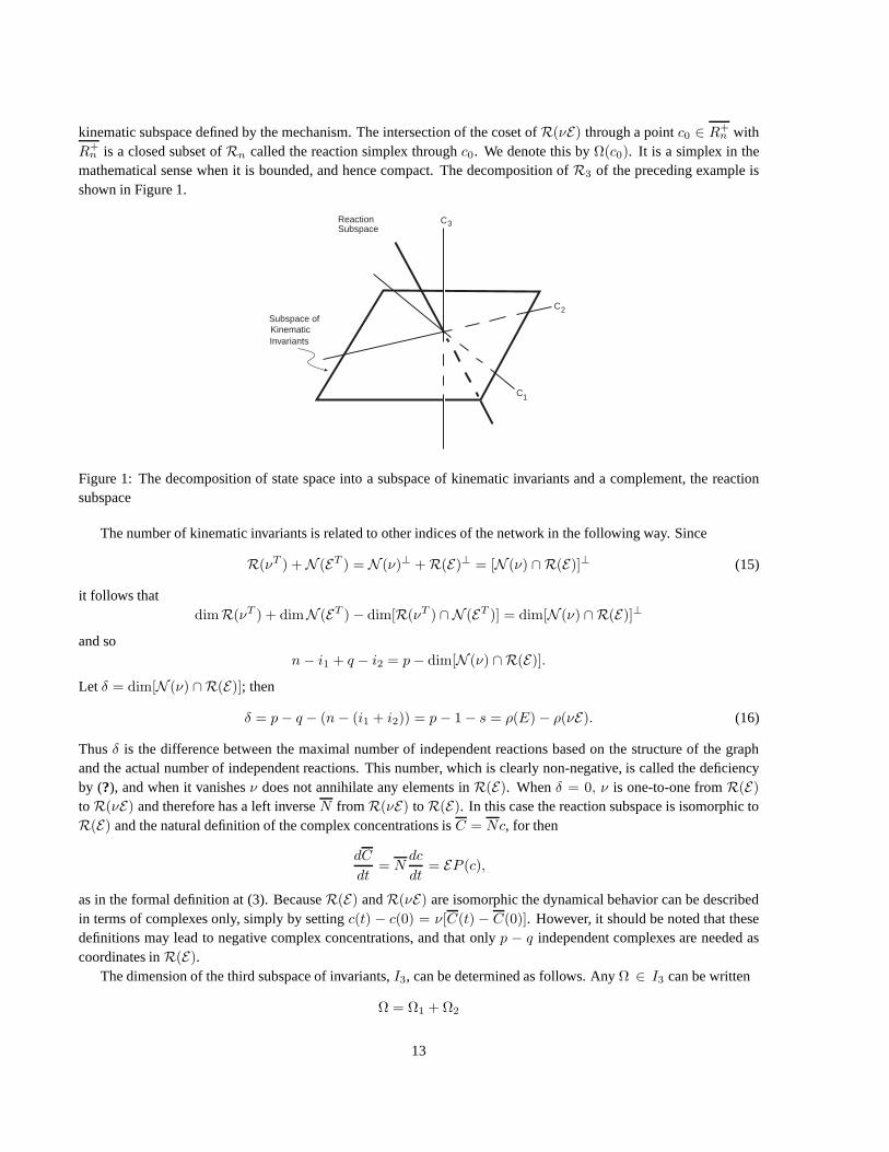
mathematical sense when it is bounded, and hence compact. The decomposition ofR3 of the preceding example isshown in Figure 1.
ReactionSubspace
Subspace ofKinematicInvariants
C1
C2
C3
Figure 1: The decomposition of state space into a subspace ofkinematic invariants and a complement, the reactionsubspace
The number of kinematic invariants is related to other indices of the network in the following way. Since
R(νT ) +N (ET ) = N (ν)⊥ +R(E)⊥ = [N (ν) ∩R(E)]⊥ (15)
it follows thatdimR(νT ) + dimN (ET )− dim[R(νT ) ∩ N (ET )] = dim[N (ν) ∩R(E)]⊥
Thusδ is the difference between the maximal number of independentreactions based on the structure of the graphand the actual number of independent reactions. This number, which is clearly non-negative, is called the deficiencyby (?), and when it vanishesν does not annihilate any elements inR(E). Whenδ = 0, ν is one-to-one fromR(E)
toR(νE) and therefore has a left inverseN fromR(νE) toR(E). In this case the reaction subspace is isomorphic toR(E) and the natural definition of the complex concentrations isC = Nc, for then
dC
dt= N
dc
dt= EP (c),
as in the formal definition at (3). BecauseR(E) andR(νE) are isomorphic the dynamical behavior can be describedin terms of complexes only, simply by settingc(t) − c(0) = ν[C(t) − C(0)]. However, it should be noted that thesedefinitions may lead to negative complex concentrations, and that onlyp − q independent complexes are needed ascoordinates inR(E).
The dimension of the third subspace of invariants,I3, can be determined as follows. AnyΩ ∈ I3 can be written
Ω = Ω1 + Ω2
13
whereΩ1 ∈ N (ET νT ) andΩ2 ∈ R(νE). Therefore
< ET νT Ω, P (c) >=< Ω2, ν E P (c) >
as before, and so it is necessary that eitherP2(c) ≡ 0, in which caseP (c) is identically proportional to an orientedcycle, or the cutset part must satisfy
< Ω2, ν E P2(c) >= 0.
The latter requires that eitherΩ2 = 0, which means thatΩ 6∈ I3, orν EP2(c) must vanish identically. Consequently,i3is certainly zero ifδ = 0 andG is acyclic, and ifδ > 0, i3 > 0 only if the cutset part is such thatEP2(c) ∈ N (ν) forall c ∈ R+
n . Thereforei3 ≤ δ whenever it is positive, anddc/dt ≡ 0 in this case. Obviously this is a very degeneratesituation, as the following example illustrates.
Suppose that the mechanism is
A0 1−→ A
B0 2−→ B
A + B3−→ C
C4−→ C0,
whereA0, B0 andC0 are held constant. We order the active species in alphabetical order, identifyA0, B0 andC0
with C(5), and label the remaining complexes as
C(1) = A
C(2) = B
C(3) = C
C(4) = A + B.
The graphG is
2
4 3 5
1
3 4
2
1
and so(p, q, r) = (5, 1, 4). One finds that
ν =
1 0 0 1 0
0 1 0 1 0
0 0 1 0 0
E =
1 0 0 0
0 1 0 0
0 0 1 −1
0 0 −1 0
−1 −1 0 1
and it follows thatρ(E) = 4, ρ(νE) = 3, andi1 = i2 = 0. SinceG is a tree,P1(c) = 0, and some computation showsthati3 = 1 if and only ofP = P2 has the form
P (c) = λ(c)
1
1
1
1
whereλ(c) 6≡ 0. Thus if all the rates are the same function ofc, every point inR+n is a steady state composition.
Needless to say, it is very rare thati3 > 0.
14
4.2 Mass Action and Related Types of Rate Functions.
A special but important class of rate functions is that in which the rate of theith reaction can be written
Pi(c) = kijRj(c)i = 1, . . . r
j = 1, . . . p(17)
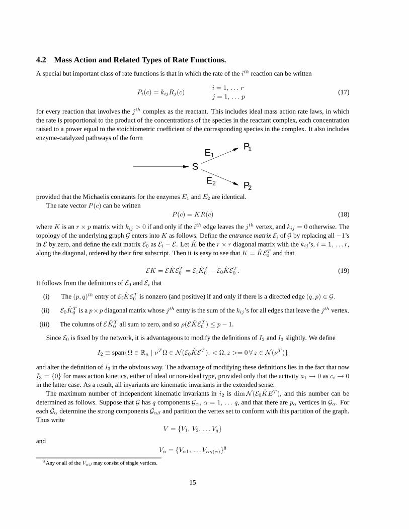
for every reaction that involves thejth complex as the reactant. This includes ideal mass action rate laws, in whichthe rate is proportional to the product of the concentrations of the species in the reactant complex, each concentrationraised to a power equal to the stoichiometric coefficient of the corresponding species in the complex. It also includesenzyme-catalyzed pathways of the form
S
P
P
11
22E
E
provided that the Michaelis constants for the enzymesE1 andE2 are identical.The rate vectorP (c) can be written
P (c) = KR(c) (18)
whereK is anr × p matrix with kij > 0 if and only if theith edge leaves thejth vertex, andkij = 0 otherwise. Thetopology of the underlying graphG enters intoK as follows. Define theentrance matrixEi of G by replacing all−1’sin E by zero, and define the exit matrixE0 asEi − E . Let K be ther × r diagonal matrix with thekij ’s, i = 1, . . . r,along the diagonal, ordered by their first subscript. Then itis easy to see thatK = KET
0 and that
EK = EKET0 = EiK
T0 − E0KE
T0 . (19)
It follows from the definitions ofE0 andEi that
(i) The (p, q)th entry ofEiKET0 is nonzero (and positive) if and only if there is a directed edge(q, p) ∈ G.
(ii) E0KT0 is ap×p diagonal matrix whosejth entry is the sum of thekij ’s for all edges that leave thejth vertex.
(iii) The columns ofEKT0 all sum to zero, and soρ(EKET
0 ) ≤ p− 1.
SinceE0 is fixed by the network, it is advantageous to modify the definitions ofI2 andI3 slightly. We define
I2 ≡ spanΩ ∈ Rn | νT Ω ∈ N (E0KE
T ), < Ω, z >= 0 ∀ z ∈ N (νT )
and alter the definition ofI3 in the obvious way. The advantage of modifying these definitions lies in the fact that nowI3 = 0 for mass action kinetics, either of ideal or non-ideal type,provided only that the activitya1 → 0 asci → 0
in the latter case. As a result, all invariants are kinematicinvariants in the extended sense.The maximum number of independent kinematic invariants ini2 is dimN (E0KET ), and this number can be
determined as follows. Suppose thatG hasq componentsGα, α = 1, . . . q, and that there arepα vertices inGα. ForeachGα determine the strong componentsGαβ and partition the vertex set to conform with this partition of the graph.Thus write
V = V1, V2, . . . Vq
andVα = Vα1, . . . Vαγ(α)
8
8Any or all of theVαβ may consist of single vertices.
15
whereγ(α) is the number of strong components inGα. TheVj are disjoint and the edge set can be partitioned in thesame way asV ; thusEKET
0 has the direct sum decomposition
EKET0 = ⊕α E
αKα (Eα0 )T
whereEα is the incidence matrix forGα. The partition ofG into components leads to the decompositions
C0 = ⊕αC0α
C1 = ⊕αC1α
(20)
whereC0α has dimensionpα andC1α has dimensionrα. It follows that we need only considerρ(EαKαEαT0 ) for a
fixedα, for the results will be additive inα. For simplicity we suppress theα onE andK until further notice.The strong componentsGαβ in the partition ofGα are of three types, namely,
(i) those in which no edges from other strong components terminate; such strong components are calledsources
(ii) strong components on which edges from other strong components terminate and from which edges to otherstrong components originate; these are calledinternalstrong components
(iii) those from which no edges to other strong components originate; these are calledabsorbingstrong compo-nents orsinks.
Clearly no vertex in a source is reachable from any vertex outside its component and no vertex in a sink is reachablefrom a vertex in any other sink. Thus the relationship of reachability defines a partial order on the strong components
of Gα, and this in turn leads to the acyclic skeleton
Gα of Gα, which is defined as follows. Associate a vertex
Vj with
each strong component ofGα, and introduce a directed edge from
Vi to
Vj if and only if one (and hence every) vertex
in Vαj is reachable fromVαi.
Gα is connected sinceGα is connected, but it is acyclic; in fact, it is a directed tree.
Either
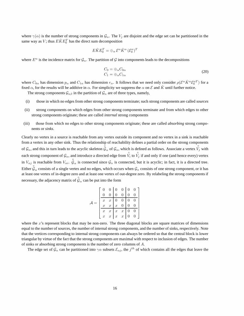
Gα consists of a single vertex and no edges, which occurs whenGα consists of one strong component, or it hasat least one vertex of in-degree zero and at least one vertex of out-degree zero. By relabeling the strong components if
necessary, the adjacency matrix of
Gα can be put into the form
A =
0 0 0 0 0 0
0 0 0 0 0 0
x x 0 0 0 0
x x x 0 0 0
x x x x 0 0
x x x x 0 0
where thex’s represent blocks that may be non-zero. The three diagonalblocks are square matrices of dimensionsequal to the number of sources, the number of internal strongcomponents, and the number of sinks, respectively. Notethat the vertices corresponding to internal strong components can always be ordered so that the central block is lowertriangular by virtue of the fact that the strong components are maximal with respect to inclusion of edges. The numberof sinks or absorbing strong components is the number of zerocolumns ofA.
The edge set ofGα can be partitioned intoγα subsetsEαj , thejth of which contains all the edges that leave the
16
vertices in thejth strong component, and the incidence matrix can then be written as follows.
E =
E11 0 0 0 0 0
0 E22 0 0 0 0
E31 E32 E33 · · · 0
E41 E42 E43 E44 · · · 0
E51 E52 E53 E54 E55 0
E61 E62 E63 E64 0 E660
(21)
(For illustrative purposes, we have writtenE for a case in which there are two each of sources, sinks and internal strongcomponents.) The non-zero elements in the off-diagonal blocks are all+1, and sinceE0 is formally obtained fromEby dropping+1’s and changing the sign of−1’s, it follows that
E0 =
E110 0 0 0 0 0
0 E220 · · · 0
0 0 E330 · · · 0
0 0 0 E440 · · · 0
0 0 0 0 E550 0
0 0 0 0 0 E660
(22)
If K andx are partitioned in conformance withE , then the system
EKET0 x = 0
can be written in the block form
E11K1ET110 0 0 0 0 0
0 E22K2ET220 0 0 0 0
E31K1ET110
... E33K3ET330 0 0 0
... E43K3ET330 E44K4ET
440 0 0... E55K5ET
550 0
E61K1ET110 .... . 0 E66K6E
T660
x1
x2
x3
x4
x5
x6
= 0.
Therefore the first step in findingdimN (E0KET ) is to determine the rank of each of the diagonal blocks.The diagonal blocksEjj of E are not the incidence matrices of a subgraph but they can be decomposed as
Ejj = [Ej1 | Ej2],
whereEj1 is the incidence matrix corresponding to all edges that originate and terminate withinGαj , whileEj2 corre-sponds to edges that originate inGαj but terminate in another strong component ofGα. Similarly,
Ejj0 = [Ej10 | −Ej2]
and soEjjKjE
Tjj0 = Ej1K − jET
j10 − Ej2KjETj2.
For every absorbing strong componentEj2KjETj2 is absent, and consequently,Ej1KjET
j10 corresponds to a strongly-
connected subgraph consisting of the edges that originate and terminate within the component. The rank ofEj1KjETj10
for such components is one less than the number of vertices inthe component, as is shown in the following proposition.
17
Proposition 1 If Gα is strongly connected, thenρ(EKET0 ) = pα − 1.
Proof. : From properties (i) and (ii) ofEKET0 given earlier, it follows that fors sufficiently large,A(s) ≡ EKET
0 +sI
is non-negative. SinceGα is strongly connected,EKET0 is irreducible (cf. (Berman and Plemmons 1979)) and so is
A(s). Therefore the Perron rootr(A) is such that
minj
∑
i
Aij ≤ maxj
∑
i
Aij
with equality on either side if and only if the minimum and maximum sums are equal (Seneta 1973; Berman andPlemmons 1979). Since these sums ares, r(A) = s and it follows thatEKET
0 has a simple zero eigenvalue;i.e. ,ρ(EKET
0 ) = pα − 1.
We know thatET u = 0 whereu = (1, . . . , 1)T , and therefore the left eigenvector ofEKET0 associated with the zero
eigenvalue isu.The foregoing shows that for anyGα,
ρ(EKET0 ) ≤ p− (# of absorbing strong components).
In fact this is an equality, as is shown next. For every non-absorbing strong component,Ej2KjETj2 is a diagonal matrix
with non-negative diagonal elements, and therefore
B(s) ≡ Ej1KjETj0 − Ej2KjE
Tj2 + sI
is non-negative for sufficiently larges. SinceEj1 is the incidence matrix of a strong component,B(s) is irreducibleand the Perron root is again bounded between the maximum and minimum column sums. Since at least one edgeleaves every non-absorbing strong component, there existsanε > 0 such that
s− ε ≤ r(B) ≤ s.
Therefore the spectrum ofEj1KjETj0−Ej2KjET
j2 lies strictly within the left-half plane, and so the diagonal blocks cor-
responding to non-absorbing strong components are all non-singular. Consequently, for everyx ∈ N (EKET0 ), xi = 0
if the ith component is non-absorbing, which proves thatdimN (EKET0 ) is equal to the number of absorbing strong
components inGα. By adding the results over all components ofG one obtains the following theorem.
Theorem 2 Let G be a graph withq componentsGα, and letNα be the number of absorbing strong components inGα. Then9
N ≡ dimN (EKET0 ) = dimN (E0KET ) =
q∑
α=1
Nα. (23)
The theorem provides an upper bound fori2 but the actual number can only be determined after the stoichiometryis specified. It should be noted that because the number of strong absorbing components ofG is at leastq, N ≥
q = dimN (ET ). Consequently, if anyGα has more than one absorbing strong component then it can happen thati2 > dimN (ET ), which would indicate that the subspaceI2 for mass-action-type rate functions contains invariantsthat would appear inI3 if the definitions of the preceding section were applied.
9HereE andK refer to the entire graphG
18
4.3 Compactness of the Reaction Simplex.
In closed systems the total mass of the mixture is conserved,and as a result, there is anΩ > 0 in N (ET νT ). This inturn implies thatΩ(c0) is bounded, and hence compact, and an application of Brouwer’s fixed point theorem showsthat there is at least one equilibrium point (Wei 1962). A similar conclusion holds for open systems when a positiveΩ exists, as the following proposition due to Horn and Jackson(1972) shows. To avoid the trivial situation in whicheveryc ∈ R+
n is a steady state, we assume hereafter thati3 = 0.
Proposition 3 Let 0 < c0 <∞ be given. ThenΩ(c0) is bounded, and hence compact, if and only if there is anΩ > 0
in N (ET νT ).
Proof. : Suppose that there is anΩ > 0 in N (ET νT ). Since the components ofΩ are finite,
< Ω, c >=< Ω, c0 ><∞,
and the intersection of this hyperplane withR+n is necessarily a bounded set. Conversely, suppose thatΩ(c0) is
bounded. SinceΩ(c0) = c0 +R(νE) ∩R+
n
it follows thatR(νE) ∩R+
n = 0
becauseΩ(c0) is bounded. The existence of anΩ > 0 is now a direct consequence of an alternative theorem due toStiemke (1915), which asserts that either the system
ET νT Ω = 0 (24)
has a solutionΩ > 0 or the systemνEz ≥ 0 (25)
has a solutionz, but never both. As was noted earlier, there is noΩ ≥ 0 in I1, and thereforeΩ(c0) is compact if and
only ifνT Ω = u (26)
has a positive solution. Hereu is given by(14), in which the scalarsωj are now non-negative. It is permissable thatsomeωj = 0, but only if the corresponding columns ofνT are zero. However, the latter means that some species donot appear in any complexes and without loss of generality they can be ignored. Therefore we require thatωj > 0 forall j.
Let U be thep× q matrix given by
U =
u1 0 . . . 0
0 u2 .
. 0 .
. . .
. .
. . .
0 0 uq
Then the problem of solving (25) is equivalent to finding a solution (Ω, ω) > (0, 0) of the system
[νT | −U ]
(
Ω
ω
)
= 0. (27)
19
By Stiemke’s theorem, this has a positive solution if and only if the system[
ν
−UT
]
x ≥ 0 (28)
has no solution.
Proposition 4 If there is at least one null complex in the network, then (26)(or (27)) does not have a positive solution.
Proof. : First suppose thatq = 1 and that there arep1 null complexes. Write
ν = [ν1 | 0]
whereν1 is n x (p-p1), and partitionx to conform with the partition ofν. Then (28) reads
ν1x1 ≥ 0
p−p1
∑
i=1
x1i +
p1
∑
j=1
x2j ≤ 0.
The first of these is satisfied if we choosex = (1, 1 . . . 1)T and the second can be satisfied by an appropriate choiceof x2. Therefore (27) has a solution and so (26) has no positive solution.
Whenq > 1, suppose that there is exactly one null complex, and by relabeling if necessary, suppose that it appearsin the first component. Partition the vertex set ofG as in Section 3.2 and partitionν to conform with the partition.Then
ν = [[ν1 | 0] | ν2 | . . . | νq]
and given a conformal partition ofx, (28) becomes
ν1x11 +
q∑
j=2
νjxj ≥ 0 (29)
p1−p1
∑
j=1
(x11)j +
p1
∑
k=1
(x12)k ≤ 0 (30)
pα∑
k=1
xαk ≤ 0 α = 2, . . . q. (31)
If we choosexα = 0, α = 2, . . . q, then (31) is satisfied and (29) and (30) are identical to the equations forq = 1. Thisproves the proposition when there is only one null complex, and an analogous argument covers the general case.10
The consequence of this result is that when there are null complexes in the network one cannot asserta priori that apositive steady state exists. The following example illustrates why one cannot expect to do better using stoichiometricinformation alone. Suppose that the reaction network is
A0 2−→ A
1−→ B
3−→ B0
10As will be shown later, a network with more than one null complex can always be transformed into an equivalent network withone nullcomplex.
20
and that reaction 1 is enzyme-catalyzed and follows Michaelis-Menten kinetics. If the rate of the input reaction isconstant and exceeds theVmax of the enzyme, the concentration ofA will simply increase monotonically and therewill be no steady state.
Another class of mechanisms for which (25) has no positive solution is given by the following proposition. Withoutloss of generality we assume that there are no null complexesin the network.
Proposition 5 Suppose that the complexes of a network are distinct and thatthe stoichiometric vectors of two com-plexes in the same component ofG are proportional. Then there is noΩ > 0 in N (ET νT ).
The proof is left to the reader. It is not true that proportionality of complexes in different components precludes theexistence of anΩ > 0, a fact that is demonstrated by a mechanism due to (Wegscheider 1902).
A1
1−→←−2
A2 2A1
1−→←−2
2A2
It is easily shown thatN (ET νT ) = span(1, 1)T for this mechanism.It is more difficult to identify general classes of systems for which there exists anΩ > 0, but here is one example.
Suppose thatp ≤ n and that the complexes are independent. Then (26) has a solution but generally it is not positive.However, ifνT has the form
νt = [A0 | A1]
whereA0 is p× p andρ(A0) = p, then
νT Ω = [A0 | A1]
(
Ω1
Ω2
)
= A0Ω1 + A1Ω2 = u
and soΩ1 = A−1
0 (u−A1Ω2).
If Ω2 > 0 , thenA1Ω2 > 0 andu − A1Ω2 can be made positive by choosing theωj ’s sufficiently large. ThereforeΩ1 > 0 if A−1
0 is non-negative. It is difficult to characterize the class ofmatrices that have a non-negative inverse,but it certainly contains the diagonal matrices with positive diagonal elements. This will be true ofA0 whenever thespecies and complexes can be ordered so that theqth complex,q = 1, . . . p, contains at least theqth species andperhaps one or more of the(p + 1)st throughnth species. Evidently this is true if all complexes are non-constantspecies.
5 Dynamical Equivalence of Networks.
The stoichiometric and incidence matrices associated witha network are fixed once a choice of complexes and reac-tions is made, but even if the reactions are all elementary, they need not be independent. This raises the more generalquestion as to what transformations of the complexes, reactions and rate functions preserve the dynamical behav-ior of the network. The dynamical behavior is completely determined by the triple(ν, E, P (c)), and two networkscharacterized by(ν, E, P (c)) and(ν′, E′, P ′(c)) respectively, are said to bedynamically equivalentif
(i) The domains ofP (c) andP ′(c) are identical.and(ii) νEP (c) = ν′E′P ′(c) for all c in the domain ofP .
If one side of the equation in (ii) vanishes identically theyboth must, and thereforei3 is invariant under trans-formations that preserve equivalence (equivalence transformations hereafter). It follows from (10) that the subspacespanned by the kinematic invariants is also unchanged, and this implies that bothi1 + i2 and the reaction subspaceremain fixed.
Three types of equivalence transformations are of interesthere, namely
21
(1) The identification of equal complexes.
(2) The removal of cycles in the graph.
(3) The removal of elements inN (ν) ∩R(E).
The first of these leavesr fixed and changesp and perhapsq, the second changesr and leavesp andq fixed, and thethird changesr and perhapsp andq. The first type is not as trivial as it may appear to be at first glance, because ’equal’complexes need only be equal with respect to the time-dependent species.
Let ν(.) denote a column ofν. let E(.) denote a row ofE, and suppose thatν(i) = ν(j) for some pair(i, j), i 6= j.Then
νE =[
ν(1) . . . ν(i) ν(j) . . . ν(p)
]
E(1)...E(p)
can be contracted to
ν′E ′ = [ν(1) . . . ν(i) . . . ν(p)]
E(E)
...E(i) + E(j)...E(p)
E ′ is the incidence matrix of a graphG′ derived fromG by moving all edges incident at vertexj to vertexi anddeleting vertexj. G′ may have cycles even ifG is acyclic, but because the reactionC(i)→ C(j) is not admitted whenν(i) = ν(j), G′ has no cycles of length one. Furthermore, if bothi andj react tok, G′ will have two edges fromi tok. This creates a cycle, which is removed in the next step. In any case,νE = ν′E ′, and since thePi’s are unchanged,the foregoing is an equivalence transformation. By applying this identification procedure repeatedly if necessary, thenumber of null complexes in a network can always be reduced toone.
The removal of cycles, which are elements inN (E), proceeds as follows. Choose a spanning tree inG and write
E = [E2 | E1]
whereE1 contains the edges in the chosen tree. A set ofp − q independent cutsets can be chosen so that every edgeof the tree is in one and only one cutset, and so that the orientation of the cutset through a tree edge agrees with theorientation of the tree edge. The resulting cutsets comprise afundamental setand the cutset matrix for this set is
Q = [Q1 | I], (32)
whereQ1 contains the edges not in the tree. Since an edge of the tree intersects exactly one cutset, it is easy to see thatE2 = E1Q1, and therefore
E = E1[Q1 | I]. (33)
Consequently,νEP (c) = νE1[Q1 | I]P (c) = νE1P
′(c) (34)
whereP ′(c) = [Q1 | I]P (c). (35)
SinceE1 is the incidence matrix for a tree, the new network, whose incidence matrix isE1, contains no cycles.However, in removing the cycles we have to reassign the rateson edges not in the tree to the tree edges. The definition
22
of P ′(c) shows that the new rate on a tree edge is the sum of the signed rates associated with the edges in the uniquecutset containing the tree edge, with the sign of each rate inthe sum fixed by the orientation of the corresponding edge.
Finally, we remove the elements inN (ν) ∩ R(E). Suppose that the intersection is spanned byδ column vectorsE(j) and that
E(j) =
p−q∑
i=1
dijE(i)1
whereE(i)1 is theith column ofE1. Since there are no elements of the formE(i)
1 ∈ N (ν) after equal complexes areidentified, we can assume without loss of generality that thefirst p − q − δ columns ofE1 span the complement ofN (ν) ∩R(E) in R(E). Then
EP (c) = E1[Q1 | I]P (c) = E1P ′′(c)
= E1DD−1P ′′(c) = E ′′P ′′ ′(c)
whereD is defined so thatE ′′ = E1D = [E(1) . . .E(p−q−δ) E(1) . . . E(δ)].
The matrixE ′′ is not the incidence matrix of a graph in general, but we recover one from it by dropping the lastδ columns. The truncatedE ′′, which we callE ′, defines the graph of the networkG′ equivalent toG. Of course thelastδ rows ofD−1 must also be dropped, and the resulting vectorP ′ gives the rate vector forG′. It can happen thatin the reduced system there are non-reacting complexes, as indicated by zero rows inE ′. These can be removed fromν andE ′ can be collapsed vertically. It should also be noted that we do not remove allz ∈ N (ν), but only those inN (ν)∩R(E). Certain dependencies between complexes are dynamically irrelevant, and whenδ = 0 they all are. Theforegoing shows thatevery network is dynamically equivalent to one for whichδ = 0.
A concrete example will illustrate the effect of the transformations. Consider the Prigoine-Lefever mechanism
A→ X → E
B + X → Y + D
2X + Y → 3X
(36)
whereinA, B, D andE are held constant. With the obvious definition of complexes,this can be written
C(5)1−→ C(1)
2−→ C(6)
C(7)3−→ C(2)
C(3)4−→ C(4).
The first step is to identifyC(5) with C(6) andC(7) with C(1). Then the graph is
C(5)1−→←−4
C(1)2−→ C(2)
C(3)3−→ C(4)
and to obtain a spanning tree simply drop reaction 1. We orderthe edges in their natural order and then find that
Q =
0 1 0 0
0 0 1 0
−1 0 0 1
E1 =
−1 0 −1
1 0 0
0 −1 0
0 1 0
0 0 1
23
and
ν =
[
1 0 2 3 0
0 1 1 0 0
]
It follows thatρ(νE) = 2, which implies that there are no kinematic invariants, as could be predicted from Proposition3. Sinceρ(E) = p− 1 = 3, δ = 1 and one finds that
N(ν) ∩R(E) = span(−1, 1− 1, 1, 0)T.
If we choose to retain reactions 2 and 4, then
D =
1 0 1
0 0 1
0 1 0
and some elementary computations show thatG′ is given by
C(5)−P1+P4←− C(1)
P2−P3−→ C(2)
where the rates are as indicated. If we retain reactions 3 and4 thenG′ is
C(1)−P1+P4−→ C(5)
C(3)−P2+P3−→ C(4)
The reader can analyze the remaining possibility.The foregoing example shows that the number of complexes andthe number of components may be different in
two equivalent networks, each of which hasδ′ = 0, distinct complexes, and an acyclic graph. Of course these numbersare not independent, becauses is invariant under equivalence transformations and so whenδ′ = 0, q′ = p′ − s.However,r′ is the same for equivalent networks if both are acyclic.
We noted earlier thati1 + i2 is invariant under equivalence transformations, but in fact bothi1 andi2 are separatelyinvariant. Identifying equal complexes changes the numberof rows ofνT but only removes redundant equations inthe systemνT Ω = 0, and therefore does not alterdimN (νT ). Thusi1 remains fixed and so also doesi2.
6 Necessary Conditions for the Existence of a Steady State.
6.1 The Relationship Between Local and Global Deficiency.
When there is no positiveΩ in N (ET νT ), as happens for instance when there are null complexes in thenetwork,arguments for the existence of a steady state based on the compactness of the reaction simplex are not applicable,and it is much harder to answer the existence question affirmatively. Indeed, it is easier to give sufficient conditionsfor the absence of any steady state, and such conditions are derived in this section. From an analytical standpoint itis easier to treat the case in which thePi’s are nonnegative, and therefore we assume at the outset that any networktransformations that are made preserve this nonnegativity.
It can be seen from (4) that there are three distinct classes of steady statescs of the network, defined by the sets
S0 ≡ cs ∈ R+
n | P (cs) = 0
S1 ≡ cs ∈ R+
n | EP (cs) = 0, P (cs) ≥ 0 (37)
S2 ≡ cs ∈ R+
n | νEP (cs) = 0, EP (cs) 6= 0.
24
The first of these is empty when there are non-vanishing constant inputs to the network. Furthermore, since theforward and reverse reactions of a reversible pair are treated separately, a steady state for such a reaction pair wouldfall into this class only if the rate of each reaction vanished separately. This would be unusual but it can happen inautocatalytic reactions or in reactions involving threshold phenomena.
The net rate of formation of each complex, as formally definedby (3), vanishes at a steady state in the secondclass. In circuit-theoretic terms, the flux ofC(i) into theith vertex balances the flux away from theith vertex andKirchoff’s current law applies (Oster and Perelson 1974). In the terminology used by Horn and Jackson (1972), thesystem iscomplex balancedat steady states inS1. At anycs ∈ S2, the rate of formation of each species vanishes butthere exists at least one vertex in the graph at which the net flux of the complex in nonzero.
Suppose, as in Section 3.2, thatG hasq components, and letPα be the number of vertices inGα. Order thecomplexes in accordance with the partition ofG into components and partitionν, E and P to conform with thisordering; then (4) can be written
dc
dt= [ν1 | ν2 | . . . νq]
E1 0
E2
0 Eq
=∑
α
ναEαPα. (38)
Hereνα is n × p, Eα is pα × rα, andPα is rα × 1, whererα is the number of reactions inGα. EachEα is theincidence matrix for the corresponding subgraphGα andρ(Eα) = pα − 1. As before, the partition leads to a directsum decomposition ofC0 andC1.
The columns of eachναEα are the stoichiometric vectors for the reactions inGα, and the number of these that areindependent, call itsα, is given byρ(ναEα). Sinceρ(Eα) = pα− 1, Sylvester’s law (Minc and Marcus 1964) impliesthatsα cannot exceedpα − 1. Thelocal deficiencyδα is defined as
δα = pα − 1− sα
= dim R(Eα)− dim R(ναEα)
= dim[N (να) ∩R(Eα)]
and it vanishes if and only if the number of independent reactions inGα is exactly the number set by the graph structure,namely,pα− 1. The total number of independent reactions computed for allcomponents isρ(νE) and it follows from(36) that
s = ρ(νE) ≤∑
α
sα ≤ p− q.
Therefore the global deficiencyδ is
δ = p− q − s ≥ p− q −∑
sα =∑
α
δα
and sinceδα ≥ 0, δ = 0 implies thatδα = 0, α = 1, . . . q, but not conversely. For future reference, we summarizethese facts and others in the following proposition.
Proposition 6 Let G be the graph of a reaction network withp complexes,r reactions andq components. Then
(i) rα ≥ pα − 1 ≥ sα
r ≥ p− q ≥ s
(ii) δα = pα − 1− sα ≥ 0
δ = p− q − s ≥∑
δα ≥ 0
(iii) s =∑
sα if and only if δ =∑
δα.
25
(iv) δα = 0 iff N (να) ∩R(Eα) = 0
δ = 0 iff N (ν) ∩R(E) = 0
(v) δ = 0 impliesδα = 0, α = 1, . . . q.
It follows from (i) that the number of dependent reactionsrα−sα in componentα is at least as large as the numberof oriented cycles inGα, and likewise for the entire graph. The excess numberδα certainly vanishes if the complexesin that component are independent, but this is not a necessary condition. The strongest conclusions that can be reachedare as follows.
Proposition 7 Let G be as in Proposition 5. Then
(i) if there is exactly one null complex inGα and ifdim N (να) = 1, thenδα = 0
(ii) if δα = 0 thendimN (να) ≤ 1
(iii) if δ = 0 thendimN (ν) ≤ q
(iv) If δα = 0, α = 1, . . . q, and if the set of non-null complexes for the entire network is linearly independent, thenδ = 0.
Proof: Let Kα ≡ C+0α ∪ −C+
0α. Since∑
i yi = 0 for anyy ∈ R(Eα),
R(Eα) ∩Kα = 0
and thereforeδα = 0 if all x ∈ N (να) lie in Kα. If dimN (να) = 1 and there is exactly one null complex inGα,which we label as thepth
α , then(0, 0, . . .0, 1)T ∈ N (να) and thereforeδα = 0.If δα = 0 thenR(Eα) ∩ N (να) = 0, and sinceN ((Eα)T ) ∩ N (να) = 0, it follows thatdimN (να) ≤
min1, pα − 1. Since there are no non-reacting complexes,pα ≥ 2 and consequently,
dimN (να) ≤ 1.
If δ = 0, a modification of the foregoing shows that
dimN (ν) ≤ minq, p− q
and sincepα ≥ 2, p ≥ 2q. ThereforedimN (ν) ≤ q.
Under the conditions in (iv),ρ(νE) =
∑
α
ρ(ναEα) =∑
ρ(Eα) = ρ(E).
It follows from (ii) that δα > 0 if there is more than one dependent complex in any component.However, we knowfrom Section 4 that whenever the dependencies are due to the presence of several null complexes, the network isdynamically equivalent to one with only one null complex. IfdimN (να) = 1 for every component in the newgraph, the according to (i),δα = 0 for every component. The conclusions in (i) and (ii) are the best possible in thatdimN (να) = 1 does not by itself imply thatδα = 0. This is illustrated in the following example. Suppose that(n, p, q, r) = (2, 3, 1, 2) and thatG, ν, andE are as follows.
1
1
2
2 3
26
ν =
[
ν11 ν12 ν13
ν21 ν22 ν23
]
E =
−1 −1
1 0
0 1
Suppose thatρ(ν) = 2, and thatν(3) = αν(1) + βν(2).
One finds thatdet νE = (1− (α + β))[ν11ν22 − ν12ν21], and consequently
δ =
0 if α + β 6= 1
1 if α + β = 1.
If α andβ are non-zero andα + β 6= 1, the example also illustrates the fact that linear independence of the non-nullcomplexes is not a necessary condition for havingδ = 0. However, according to (ii) and (iii) of Proposition 7, therecan be at most one linear relation between the stoichiometric vectors of the complexes in componentα if δα is tobe zero, and at mostq overall if δ is to be zero. Because
∑
yi = 0 for any y ∈ N (Eα), the most general linearrelationship between the complexes that is compatible withδα = 0 is of the form
p∑
i=1
yαi να
(i) = 0,
p∑
i=1
yαi 6= 0. (39)
If these are satisfied for allα and there are no inter-component relations of the form
p∑
i=1
yiν(i) =,
p∑
i=1
yi = 0, (40)
thenδ = 0 as well. Thus an autocatalytic reaction of the form
C(i)→← λC(i) λ > 1
does not, by itself, lead to a non-zero deficiency. However, the Wegscheider mechanism discussed in Section 3 hastwo inter-component relations between the complexes and thereforeδ > 0 for this mechanism, even thoughδα = 0
for each component.
6.2 Nonexistence of Balanced Flows
At a steady statecs ∈ S2, the flowP (cs) satisfies
EP (cs) = 0, P (cs) ≥ 0,
and the partitioned form of the equations at (38) shows that
EαPα(cs) = 0 α = 1, . . . q. (41)
Consequently, the flowPα(cs) on each component ofG is a balanced nonnegative flow and is strictly nonnegativeon at least one component. Our next objective is to determinewhen such flows cannot exist, and for this purpose werequire the following special case of a theorem due to (Motzkin 1936).11
Theorem 8 Let A be a non-zero matrix. Then eitherAx = 0, x ≥ 0 has a solution orAT y > 0 has a solution, butnever both.
11The complete statement of this theorem, Stiemke’s theorem,and more general alternative theorems can be found in (Mangasarian 1969).
27
Theorem 9 Let G be the graph of a reaction network withp complexes,r reactions andq components.
(i) If G is acyclic then there exists no strictly nonnegative balanced flow.
(ii) There exists a positive balanced flow if and only if everycomponentGα of G is strongly connected.
Proof. : To prove (i), all we have to do is show that
ET y > 0 (42)
has a solution whenG is acyclic. Without loss of generality, we can assume thatα = 1, for otherwise we apply theargument to each component. In order that there be a solution, it is necessary and sufficient thaty satisfy
−yi + yj > 0 (43)
for every ordered pair(i, j) in the edge of set ofG. To construct ay that satisfies (43), we proceed as follows. SinceGis acyclic, there is at least one vertexVj with d+
j = 0 (an ’initial’ vertex) and at least oneVk with d+k = 0 (a ’terminal’
vertex). Choose a directed path from an initial vertexV1 to a terminal vertexVk and, beginning withy1 = 1, defineyk+1 = yk + 1 for those vertices on the chosen path. If there is only one such path throughG this provides the desiredy. If more than one path leavesV1, or if there is more than one initial vertex, repeat the procedure for each path. Ifmore than one path is incident at some vertexVj , assignyj the largest of the values associated with the paths incidentatVj and repeat the foregoing procedure for each path leavingVj . The resultingy satisfies (40) and this proves (i).
SinceGα is strongly connected if and only if there exists a closed directed edge sequence that contains all theedges, it follows that a positive balanced flow exists when every Gα is strongly connected. To prove the converse,we show that if someGα is not strongly connected then there exists no positive balanced flow. This will follow fromStiemke’s theorem if we can show that
ET y ≥ 0 (44)
has a solution, for thenEz = 0, z > 0
has none. We can again assume thatα = 1 without loss of generality. PartitionGα into strong componentGαβ as in3.2, and then (44) becomes
ET y =
∣
∣
∣
∣
∣
∣
∣
∣
∣
∣
∣
∣
∣
∣
∣
∣
∣
ET11 0 ET
31 ET41 ET
51 ET61
0 ET22 ET
32 ET42 ET
52 ET62
0 0 ET33 ET
43 ET53 ET
63
0 0 0 ET44 ET
54 ET64
0 0 0 0 ET55 0
0 0 0 0 0 ET66
∣
∣
∣
∣
∣
∣
∣
∣
∣
∣
∣
∣
∣
∣
∣
∣
∣
y1
y2
y3
y4
y5
y6
≥ 0.
(As before, we illustrate the case in which there are two eachof sources, sinks and internal strong components, but thearguments used apply in general.) Now recall thatE55 andE66 are the incidence matrices for strong components, andtherefore
ETjjyj ≥ 0 j = 5, 6
has no solution becauseEjjzj = 0, zj > 0
28
has a solution by virtue of the ’if’ part of (ii) applied to thesubgraphs. Furthermore, recall that the off-diagonalblocks are non-negative, and sinceGα is not strongly connected andp > 1, there is at least one such block that is notidentically zero. Therefore, if we choose
yj = 0 j = 1, . . . 4
yj = uj j = 5, 6
thenET
jjyj = 0 j = 1, . . . 6
and for at least one pair(i, j)ET
ijyj ≥ 0.
The theorem implies thatS1 can be nonempty only if at least one component ofG contain a cyclic sequence ofreactions of the form
C(1)→ C(2)→ . . .→ C(1).
’Apparent’ cycles may in fact not be cyclic in the foregoing sense. For instance, the feedback system
S0 → S1 → S2 → . . .→ Sn → Products
in which all reactions shown are irreversible, is acyclic when the rate function for the first reaction is taken to bef(Sn) · S0 (Tyson and Othmer 1978). However if the concentrations ofS0 and the products are time invariant and ifthe associated complexes are identified, the resulting network is strongly connected.
6.3 Conditions under whichS2 = φ.
The flows corresponding to steady state inS2 contains both cycles and cutsets and therefore the steady-state versionof (38) reads
0 =∑
α
ναEαPα(cs) =∑
α
ναEα[(Bα)T wα + (Qα)T zα] =∑
α
ναEα(Qα)T zα α = 1, . . . q (45)
whereinzα 6= 0 for at least oneα. The sum vanishes either if every term vanishes or if there are at least two nonzeroterms whose sum vanishes. In the former case the steady stateflow is said to belocally-compensatedbecause theunbalanced part of the flow is annihilated byναEα on every componentGα. The flow is onlyglobally-compensatedat cs in the latter case because there is at least one species in thesystem for which the net rate of production inone component ofG is compensated for by a net rate of consumption in another component. In either case the flowcan be balanced on as many asm components, wherem = q − 1 (q − 2) for a locally-compensated (globally-compensated) steady state flow. Of course all flows that are balanced are automaticlly locally-compensated, andbecauseR(E) = ⊕R(Eα), balanced flows are always balanced component-wise (in factvertex-wise).
If δαα = 0 for all α there are certainly no locally-compensated flows that are not balanced. This occurs, for instance
whenN (να) = 0 for all α, in which case the complexes within each component are independent. In order forδ tobe positive, it is necessary that(νE) ⊂ ⊕R(ναEα), i.e., the reaction subspace for the entire network must be apropersubspace of the direct sum of those for the components. Furthermore,
N (ν) = y ∈ C0 | y = (y1, . . . yq)T , νy = 0, ναyα 6= 0 for yα 6= 0 ≡ N0 (46)
in this case. E xamples of this case are given by the Prigogine-Lefevermechanism and by the Wegscheider mechanism,a special case of which will be discussed later.
29
In generalN (ν) = ⊕αN (να) ⊕ N0 (47)
and the opposite extreme occurs whenN0 = 0. Now there are no inter-component linear combinations of complexesthat are zero, and all steady-state flows that are unbalancedare necessarily locally-compensated. In order forδ to bepositive, there must be aδα 6= 0 for at least oneα, and hereR(νE) = ⊕R(ναEα). Thuss =
∑
sα and by Proposition5, δ =
∑
δα.The foregoing provides sufficient conditions for the absence of locally-compensated flows(δα = 0 for all α),
sufficient conditions under which there are no globally-compensated flows(δ =∑
δα), and sufficient conditions forS2 = φ (δ = 0). However, these conditions are not necessary, as a later example will illustrate. A sharper set ofconditions is obtained as follows. Let
Kα1 ≡ y
α ∈ C0α | yα = Eαxα, xα ∈ C1α, xα ≥ 0. (48)
Then the equationsναEαxα = 0 α = 1, . . . q (49)
have a solution for whichEαxα 6= 0 for at least oneα only if there is anα for which
N (να) ∩ Kα1 − 0 6= φ. (50)
Therefore there is no locally-compensated flow that is not balanced on at least one componentGα if and only if
N (να) ∩Kα1 = 0, α = 1, . . . q. (51)
Similarly, S2 = φ ifN (ν) ∩K1 = 0, (52)
whereK1 ≡ y ∈ C0 | y = Ex, x ∈ C1, x ≥ 0. (53)
Certainlyδα = 0 α = 1, . . . q implies (51) andδ = 0 implies (49), but not conversely, as the following exampleillustrates.
Consider again the example following Proposition 6, and suppose thatα + β = 1, which means thatδ = 1. TheconeK1 is generated by the vectors(−1, 1, 0)T and(−1, 0, 1)T andN (ν) is spanned by(α, 1 − α,−1)T . Someelementary computation shows that when0 ≤ α ≤ 1 there is no pair(λ1, λ2) with sgnλ1 = sgnλ2 such that
λ1
−1
1
0
+ λ2
−1
0
1
=
α
1− α
−1
Therefore, for this choice of(α, β)
N (ν) ∩ K1 − 0 = φ
and soS2 = φ. Moreover, sinceG is acyclic, either there is acs ∈ R+2 at which the flow on both edges vanishes or
there is no steady state.When all reactions in every component are reversible, the negative of any column ofE is also a column ofE , and
so
Eαx = [E(1) − E(1) E(2) − E(2) . . .]
x1
x2
...xr
= (x1 − x2)E(1) + (x3 − x4)E(2) + · · · ·
30
Consequently, it cannot happen thatN (να) ∩ Kα
1 = 0 (54)
even thoughδα > 0. Of course this only asserts the existence of a vectorx ≥ 0 such thatEαx 6= 0 andναEαx = 0;it does not imply that for a given choice of rate functions a steady statecs exists at which the flow is unbalanced.Another case in which (51) does not occur forδα > 0 is whenGα is strongly-connected. Then Theorem 2 shows thatthere is anx0 > 0 such thatEαx0 = 0, and given anyx1 ∈ N (να) ∩ R(Eα), let x = x1 + λx0 with λ > 0 andsufficiently large. Thusx is a locally-compensated, unbalanced, non-negative flow, but again, this is not an existenceresult for any given choice of rate functions.
Earlier we interpretedδα as the excess of the actual number of dependent reactions inGα over the number set bythe structure ofGα. An alternate interpretation is as follows. SincedimN (ναEα) = rα − sα, there existrα − sα
linearly independent flows that are annihilated byναEα. Since every oriented cycle inGα lies inN (ναEα) there are
rα − sα − (rα − pα + 1) = pα − sα − 1 = δα
independent flows inN (ναEα) that are not balanced. These are necessarily cutsets, in view of the decomposition ofC1α, and thusδα represents the maximum number of independent cutsets that can appear in any flow that is annihilatedby ναEα. Of course a particular flow need not contain that many; it could, for instance, be balanced even ifδα > 0. IfGα is a tree then every flow onGα is a linear combination of cutsets and ifδα = 0 there is no such combination thatis annihilated byναEα. In this caseS1 = φ and there are no locally-compensated steady flows forcs ∈ S2. HoweverS2 need not be empty, since there may be a globally-compensatedflow. As an example of this, consider the followingspecial case of Wegscheider’s mechanism:
M1 →M2
2M2 → 2M1.,
Let C(1) =M1, C(2) = M2, C(3) = 2M1, C(4) = 2M2. Then the graph is
41 2 3
and the stoichiometric and incidence matrices are
ν =
[
1 0 2 0
0 1 0 2
]
E =
−1 0
1 0
0 1
0 −1
It is evident thatρ(ν1E1) = ρ(E1) = 1 and thatρ(ν2E2) = ρ(E2) = 1; thus the flow cannot be locally-compensated,nor can it be balanced unless it vanishes on all edges, sinceG is acyclic. One finds thatρ(νE) = 1, soδ = 1 andS2
need not be empty. A simple computation shows that anyz0 ∈ N (ν) andz1 ∈ R(E) must have the form
z0 =
−2u
−2v
u
v
z1 =
−x
x
y
−y
whereu, v, x, y are arbitrary. Consequently
EP (cs) =
−P1(cs)
P1(cs)
P2(cs)
−P2(cs)
∈ N (ν)
31
if and only if the system
P1(cs) = λ
P2(cs) = 2λ
has a solutioncs ∈ R+2 for someλ ≥ 0. When a solution existsS2 6= φ; whether or not it does depends on the choice
of constitutive relations.
6.4 A Flow Chart For Determining Whether Any Steady State CanExist.
The foregoing leads to a prcedure for systematically deciding whether certain types of flows can exist or whether theycan be ruled out on the basis of stoichiometry and network structure alone. A schematic flow chart for such a procedureis shown in Figure 2. The conclusion that there are no positive balanced flows unless everyGα is strongly connected isessentially due to Horn (1972) and is part of the zero deficiency theorem (Feinberg 1977; Feinberg 1980). Thatδ = 0
impliesS2 = Φ also follows from Feinberg (1972), but the notions of locally- and globally-compensated flows are notused there. Neither of the foregoing authors allows rate functions that vanish at positive concentrations and the setS0
does not arise in their analyses.The problem of constructing and implementing the algorithms required for the tests in the flow chart will be dealt
with elsewhere, but some general remarks are in order. Algorithms for deciding whether a graph is strongly-connectedor acyclic exist, and the tests on the deficiency only requirea comparison of the ranks of two matrices. If the complexesare independent these ranks are obviously equal andS2 = φ. A less trivial case occurs when every non-null complexis a species, for thenN (ν) = ⊕N (να) and the rank condition can be checked separately for each componentGα.
The general problem of deciding when (48) and/or (49) are satisfied can be cast as the quadratic programmingproblem
min < νx, νx >,
x ∈ IntK1
but this aspect will not be pursued here. If all thePi are bounded above, as for instance when the reactions are allenzyme-catalyzed and Michaelis-Menten kinetics are applicable, the minimization is over a convex polyhedronK∗
1
instead of over the coneK1
7 Discussion
When there is only one independent reaction in the system, the dynamical behavior is completely described by thesolution of the scalar equationξ = f(ξ) in the extent of reaction, and a qualitative analysis is veryeasy. One canreadily determine the steady states, the transient behavior for all initial conditions, and the sensitivity of solutionswith respect to parametric changes and changes in the form off . It is evidently important to be able to obtain similarinformation about general networks, for such information would enable one to predict, for instance, how the dynamicalbehavior changes when a catalyst in some pathway is poisonedor a new pathway is added. If good techniques forobtaining this information for large systems were available, a composite performance index that measures stability,sensitivity and efficiency could be devised, and alternative synthetic pathways could be compared. Such comparisonsmight well provide insights into why existing biochemical pathways and networks built from them have evolved totheir present form. Unfortunately such techniques are not available yet, but it is clear that the ability to systematicallyanalyze how the reaction phenomenology and network structure are reflected in the dynamical equations is a steptoward their development. The graph-theoretic methods we introduce here seem to serve this purpose well.
Substantial progress has been made by others toward understanding special classes of reaction networks. Anearly attempt to obtain global results for open systems withideal mass action kinetics was made by Shear (1967).However, as Higgins (1968) pointed out, Shear’s H-function, which is actually the thermodynamic availability of the
32
∀ α?αδ = 0
δ = 0 ?
S φ=2
S φ=2
N (ν α ) ∩ K1= 0
∀ α?
N (ν ) ∩ K1= 0
Locally-compensatedflows possible
globally-compensatedflows may exist
Nolocally-compensated
flows
No
No
No
No
Yes
Yes
Yes
Yes
≤ P(c) 0∀ c?
S0
≠ φ S0
φ=No Yes
acyclicG
?
S φ=1S1 may be
nonempty
No Yes
Gα
∀ α?strong
No positivebalanced
flows
Positive
may existbalanced flows
No Yes
Figure 2: A flow chart for determining the existence of steadystates.
system relative to an assumed steady state, is not a Lyapunovfunction for all systems, as Shear had claimed. In alandmark paper, Horn and Jackson (1972) showed that if a strictly positive steady state exists, the availability is a localLyapunov function whenever the steady state flow is balanced. If one can also establish that there are no equilibria onthe boundary of the simplex, and if there is an equilibrium point in the interior of the simplex, then it is unique andglobally stable. Our formulation was originally motivatedby a desire to extend these results to networks with massaction kinetics in general, non-ideal solutions, and to identify other classes of networks for which similar conclusionscan be reached. The latter problem is particularly important in the biological context, where the rate functions in areduced description of a network are often rational functions, and feedback control within and between pathways is therule rather than the exception. We have made some progress onthe analysis of more general networks and in sequelsto this paper we will show
(i) that the availability is a local Lyapunov function for a more general class of kinetics than ideal mass-action type,provided the flow is balanced at the steady state
33
(ii) that certain networks with monotone rate functions have a unique steady state, and when they are forced pe-riodically, they have a unique periodic solution whose period is that of the driving frequency (thus sub- andsuper-harmonic solutions are ruled out.)
(iii) how the cycle structure of the Jacobian ofνEP (c) is related to the structure of the graph and the feedbackpresent, and how these affect the stability of a steady stateaccording to a linear analysis.
A by-product of our approach is that many of the results due toHorn and Jackson (1972), Horn (1972) and Feinberg(1977, 1980) can be obtained more directly. The separation of the usual stoichiometric matrix into the factorsν andE makes it clear why the caseδ = 0 is relatively easy to treat, and new interpretations of the deficiency emerge. Thegeneral representation of a balanced flow leads to an easy proof that the availability is a Lyapunov function undercertain conditions, and Theorem 2 can be used to give an easy proof of parts of the zero-deficiency theorem. This isnot to detract from previous work, but only to illustrate that the results become more transparent when the networkstructure and reaction phenomenology are separated more clearly.
Ours is not the first application of graph-theoretic techniques to the analysis of reaction networks, and in conclu-sion we shall mention some realted work. Aris (1965) developed the algebraic approach to the analysis of reactingsystems and Sellers (1966) has applied ideas from algebraictopology and graph theory to the problem. The networkthermodynamics approach developed in Oster and Perelson (1974) and Perelson and Oster (1974), in which bondgraphs are used to represent reactions, is related to Sellers’ work. The underlying graph structure is quite differentfrom ours, in that species rather than complexes are assigned to nodes, and the representation of chemical reactions ismore complicated. Horn (1973a) recognized that networks could be represented by graphs in which the nodes repre-sent complexes, but he did not exploit this fact in analyzingthe structure of the dynamical equations. He has also usedspecies graphs (those in which the nodes represent species)to analyze systems in which all complexes have at mosttwo species (Horn 1973b). Williamowski and Rossler (1978)and Williamowski (1978) have continued the latter lineof investigation and have enumerated the different types ofsecond-order, ideal, mass-action kinetic networks. Toth(1979) has obtained results on the types of systems that leadto gradient flows. (1978) and (1973) make extensiveuse of network structure in analyzing the case in which the rate functions are represented by Boolean functions. Thisapproach is useful in cases where the rate laws model switches, but in many cases this is too crude an approximationto reality.
The linear problem that arises either when the kinetics are first-order or when the stability of a steady state isinvestigated has been treated by several authors. Hill (1970) has used results from the topological analysis of linearsystems to obtain representations of the steady state concentrations and fluxes for any system of reversible first-orderreactions in terms of weights on directed trees in the graph.A similar approach can be used to represent the ratefunctionsR(cs) for any mass-action-like kinetics, provided that the flow isbalanced. Beretta et. al. (1979) useda technique due to Hyver (1980) to identify a class of mass action kinetics for which a steady state, if one exists, isalways stable according to linear theory. Their results complement those of Horn and Jackson in that it is not necessaryto assume that the deficiency is zero or that the flow is balanced. Clarke (1980) provides a comprehensive review ofhis own and related work on the stability problem. He also observes that the usual stoichiometric matrix can be writtenin factored form, as we do, but does not make use of this fact. The relation of his work on the linear problem to ourapproach will be discussed in a future paper devoted to the linear problem.
ACKNOWLEDGEMENTS
This paper is an outgrowth of a course offered at Rutgers University in early 1979. I am indebted to the participants,N. Greenbaun, Z. Kadas and P. Monk, for their questions and comments, which resulted in various extensions andclarifications. This work was partially supported under Grants GM21558 and GM 29123 from the National Institutesof Health.
34
References
Aris, R. 1962.Vectors, Tensors and the Basic Equations of Fluid Mechanics. Prentice-Hall, New York.
Aris, R. 1965. Prologomena to the rational analysis of chemical reactions.Archive for rational mechanics and analysis,19(2), 81–99.
Berman, A. and Plemmons, R.J. 1979.Nonnegative Matrices in the Mathematical Sciences. New York: AcademicPress.
Chen, W. K. 1971.Applied Graph Theory. Amsterdam: North-Holland.
DeGroot, S. and Mazur, P. 1962.Non-Equilibrium Thermodynamics. Amsterdam: North-Holland.
Denbigh, K. G. 1952. Entropy Creation in Open Reaction Systems. Trans. Far Soc., 48, 389–394.
Feinberg, M. 1977. Mathematical Aspects of Mass Action Kinetics. In: Lapidus, L. and Amundson, N. R. (eds),Chemical Reactor Theory: A Review. Englewood Cliffs: Prentice-Hall.
Feinberg, M. 1980. Chemical Oscillations, Multiple Equlibria, and Reaction Network Structure.In: Stewart, W., Ray,W. H., and Conley, C. (eds),Dynamics and Modelling of Reaction Systems. New York: Academic Press.
Giblin, P. J. 1977.Graphs, Surfaces and Homology. New York: Wiley.
Glass, L. and Kaufmann, S. 1973. The Logical Analysis of Continuous Nonlinear Biochemical Control Networks.J.Theor. Biol., 39, 103–129.
Glass, L. and Pasternack, J. S. 1978. Stable Oscillations inMathematical Models of Biological Control Systems.J.Math. Biology, pages 207–223.
Harary, F. 1969.Graph Theory. Reading: Addison-Wesley.
Heineken, F., Tsuchiya, H., and Aris, R. 1967. On the Mathematical Status of the Pseudo-steady State Hypothesis ofBiochemical Kinetics.Math. Biosciences, pages 95–113.
Hocking, J. C. and Young, G. S. 1961.Topology. Reading: Addison-Wesley.
Horn, F. 1972. Necessary and Sufficient Conditions for Complex Balancing in Chemical Kinetics.Arch. Rat. Mech.Anal., 49, 172–186.
Horn, F. 1973a. On a Connexion Between Stability and Graphs in Chemical Kinetics; I. Stability and the ReactionDiagram.Proc. Roy. Soc. Lon., A334, 299–312.
Horn, F. 1973b. On a Connexion Between Stability and Graphs in Chemical Kinetics II. Stability and the ComplexGraph.Proc. Roy. Soc. Lon., A334, 313–330.
Horn, F. and Jackson, R. 1972. General mass action kinetics.Archive for rational mechanics and analysis, 48, 81.
Mangasarian, O. 1969.Nonlinear Programming. New York: McGraww-Hill.
Mel, H. C. and Ewald, D. A. 1974. Thermodynamic Potentials and Evolution towards the Stationary State in OpenSystems of Far-from-Equilibrium Chemical Reactions: The Affinity Squared Minimum Function.Journal ofMathematical Biology, 1, 133–151.
35
Minc, H. and Marcus, M. 1964.A Survey of Matrix Theory and Matrix Inequalities. Boston: Prindle, Weber andSchmidt.
Motzkin, T. S. 1936.Beitrage zur Theorie der Linearen Ungleichungen. Inaugural Dissertation. Basel, Jerusalem.
Nagumo, M. 1942.Uber die Lage der Integralkurven Gewonlicher Differential Gleichungen.Proc. Phys. Math. Soc.Japan, 24, 551–559.
Oster, George F. and Perelson, Alan S. 1974. Chemical Reaction Dynamics Part I: Geometrical Structure.Archive forrational mechanics and analysis, 55(3), 230–274.
Othmer, H. G. 1981. The interaction of structure and dynamics in chemical reaction networks.Pages 1–19 of:Ebert,K. H., Deuflhard, P., and Jager, W. (eds),Modelling of Chemical Reaction Systems. New York, NY, USA: Spring-er-Verlag.
Sellers, Peter H. 1966. Algebraic Complexes Applied to Chemistry. Proceedings of the National Academy of Sciencesof the United States of America, 55, 693–698.
Seneta, E. 1973.Non-Negative Matrices. New York: Wiley.
Shear, D. 1967. An Analog of the Boltzmann H-Theorem (a Liapunov Function) for Systems of Coupled ChemicalReactions.Jour. Theor. Biol., 16, 212–228.
Toth, J. 1979. Gradient Systems are Cross-Catalytic.React. Kinet. Catal. Lett., 12, 253–257.
Tyson, J. J. and Othmer, H. G. 1978. The dynamics of feedback control circuits in biochemical pathways.Progress inTheor. Biol., 5, 1–62.
Vandergraft, J. S. 1968. Spectral Properties of Matrices which have Invariant Cones.SIAM J. Appl. Math., 16, 1208–1222.
Wegscheider, R. 1902.Uber Simultane Gleichgewichte und die Beziehungen Zwischen Thermodynamik und Reak-tionskinetik Homogener Systeme.A. Physik. Chem., 39, 257–303.
Wei, J. 1962. Axiomatic Treatment of Chemical Reaction Systems.Jour. Chem. Phys., 36, 1578–1584.
Williamowski, K.-D. 1978. Contributions to the Theory of Mass Action Kinetics. II. Representations of Closed andOpen Kinetics.Z. Naturforsch, 33a, 983–988.
Williamowski, K.-D. and Rossler, O. E. 1978. Contributions to the Theory of Mass Action Kinetics. I. Enumerationsof Second Order Mass Action Kinetics.Z. Naturforsch., 33a, 827–833.