Page 1
Reference Manual for GRETNA (v2.0) Page 1
A Graph Theoretical Network Analysis Toolbox
Reference Manual for GRETNA (v2.0)
June 2017
National Key Laboratory of Cognitive Neuroscience and Learning
Beijing Key Laboratory of Brain Imaging and Connectomics
IDG/McGovern Institute for Brain Research
Beijing Normal University, Beijing, China
Page 2
Reference Manual for GRETNA (v2.0) Page 2
Table of Contents
1. Overview .............................................................................................................................................................. 4
2. License ................................................................................................................................................................. 5
3. Prerequisites ........................................................................................................................................................ 5
4. Installation ........................................................................................................................................................... 6
5. Network Construction.......................................................................................................................................... 8
5.1. R-fMRI Preprocessing ............................................................................................................................... 8
5.1.1. DICOM to NIfTI ........................................................................................................................... 10
5.1.2. Remove First Images .................................................................................................................. 11
5.1.3. Slice Timing ................................................................................................................................ 12
5.1.4. Realign........................................................................................................................................ 13
5.1.5. Normalize ................................................................................................................................... 14
5.1.6. Spatially Smooth ........................................................................................................................ 17
5.1.7. Regress Out Covariates .............................................................................................................. 18
5.1.8. Temporally Detrend ................................................................................................................... 19
5.1.9. Temporally Filter ........................................................................................................................ 20
5.1.10. Scrubbing ................................................................................................................................... 21
5.1.11. Results of R-fMRI Preprocessing ................................................................................................ 22
5.2. Functional Connectivity Matrix Construction ........................................................................................ 25
5.2.1. Static Correlation ....................................................................................................................... 26
5.2.2. Dynamical Correlation ............................................................................................................... 26
5.2.3. Results of Functional Connectivity Matrix Construction ............................................................ 27
6. Network Analysis ............................................................................................................................................... 28
6.1. Global Network Metrics ......................................................................................................................... 31
6.1.1. Small-World ............................................................................................................................... 32
6.1.2. Efficiency .................................................................................................................................... 32
6.1.3. Rich-Club .................................................................................................................................... 32
6.1.4. Assortativity ............................................................................................................................... 33
6.1.5. Synchronization .......................................................................................................................... 33
6.1.6. Hierarchy .................................................................................................................................... 33
6.2. Nodal and Modular Network Metrics .................................................................................................... 33
6.2.1. Clustering Coefficient ................................................................................................................. 34
6.2.2. Shortest Path Length .................................................................................................................. 34
6.2.3. Efficiency .................................................................................................................................... 34
6.2.4. Local Efficiency ........................................................................................................................... 34
6.2.5. Degree Centrality ....................................................................................................................... 34
6.2.6. Betweenness Centrality ............................................................................................................. 35
6.2.7. Community Index ....................................................................................................................... 35
6.2.8. Participant Coefficient ............................................................................................................... 36
6.2.9. Modular Interaction ................................................................................................................... 37
6.3. Results of Network Analysis ................................................................................................................... 37
Page 3
Reference Manual for GRETNA (v2.0) Page 3
6.3.1. Global Network Metrics ............................................................................................................. 38
6.3.2. Nodal and Modular Network Metrics ........................................................................................ 41
7. Metric Comparison ............................................................................................................................................ 47
7.1. Network and Node ................................................................................................................................. 47
7.1.1. One-Sample t-Test ...................................................................................................................... 49
7.1.2. Two-Sample t-Test ...................................................................................................................... 50
7.1.3. Paired t-Test ............................................................................................................................... 51
7.1.4. One-Way ANCOVA ...................................................................................................................... 52
7.1.5. One-Way ANCOVA (Repeated Measures) .................................................................................. 53
7.1.6. Correlation Analysis ................................................................................................................... 54
7.2. Connection ............................................................................................................................................. 55
7.2.1. Averaged (Functional) ................................................................................................................ 56
7.2.2. Backbone (Structural) ................................................................................................................ 57
7.2.3. One-Sample t-Test ...................................................................................................................... 58
7.2.4. Two-Sample t-Test ...................................................................................................................... 59
7.3. Results of Metric Comparison ................................................................................................................ 60
7.3.1. Network and Node ..................................................................................................................... 60
7.3.2. Connection ................................................................................................................................. 62
8. Metric Plotting ................................................................................................................................................... 64
8.1. Bar .......................................................................................................................................................... 65
8.2. Dot ......................................................................................................................................................... 66
8.3. Violin ...................................................................................................................................................... 67
8.4. Shade ..................................................................................................................................................... 68
9. GANNM .............................................................................................................................................................. 69
Acknowledgements.................................................................................................................................................... 70
Reference ................................................................................................................................................................... 71
Page 4
Reference Manual for GRETNA (v2.0) Page 4
1. Overview
The GRETNA toolbox has been designed for the graph-theoretical network analysis of fMRI data. It
is a suite of MATLAB functions and MATLAB-based interfaces for conventional fMRI
preprocessing and for the calculation and statistical analysis of the most frequently used network
metrics, such small-world parameters, efficiency, degree, betweenness, assortativity, hierarchy,
synchronization and modularity.
Thank you for using GRETNA (v2.0.0). When using this package in your publicized work, PLEASE
CITE:
Wang, J., Wang, X., Xia, M., Liao, X., Evans, A., & He, Y. (2015). GRETNA: a graph theoretical
network analysis toolbox for imaging connectomics. Frontiers in human neuroscience, 9, 386.
Developed by Jinghui Wang and Xindi Wang
National Key Laboratory of Cognitive Neuroscience and Learning,
Beijing Normal University, China
Contact information:
Jinhui Wang: [email protected]
Xindi Wang: [email protected]
Yong He: [email protected]
Copyright © 2017 Dr. Yong He’s Lab, National Key Laboratory of Cognitive Neuroscience and
Learning, Beijing Normal University, Beijing, China.
Page 5
Reference Manual for GRETNA (v2.0) Page 5
2. License
GRETNA is distributed under the terms of the GNU General Public License as published by the Free
Software Foundation (version 3). The details on ‘copyleft’ can be found at
http://www.gnu.org/copyleft/.
3. Prerequisites
Getting started to run GRETNA on your computer:
• MATLAB: A high-level numerical mathematics environment developed by MathWorks, Inc.
Natick, MA, USA. GRETNA requires MATLAB2010a or later version.
• SPM8/SPM12: SPM is freely available to the (neuro) imaging community andrepresents the
implementation of the theoretical concepts of Statistical Parametric Mapping in a complete
analysis package. Given that the names of certain functions in SPM8/SPM12 are the same as
those in GRETNA or MATLAB, we recommend that you add only the path of the home folder of
SPM8/SPM12 when you use GRETNA.
• MatlabBGL: MatlabBGL is a MATLAB package for working with graphs. It uses the Boost
Graph Library to efficiently implement graph algorithms. GRETNA has included this package in
its distribution. Thus, you do not need to download MatlabBGL again.
• PSOM: The pipeline system for GNU Octave and MATLAB (PSOM) is a lightweight library for
managing complex multi-stage data processing. A pipeline is a collection of jobs, i.e. MATLAB
or Octave codes, with a well identified set of options that use files for inputs and outputs.
GRETNA has included this package in its distribution. Thus, you do not need to download
PSOM again.
Page 6
Reference Manual for GRETNA (v2.0) Page 6
4. Installation
Run MATLAB. You can add the GRETNA path to the MATLAB search path in one of two ways:
Command-line or Interface.
• Command-line
Type the following command in the MATLAB command window.
>>addpath(genpath(‘D:\...\GRETNA’));
where ‘D:\...\GRETNA’ is the path of GRETNA on your computer.
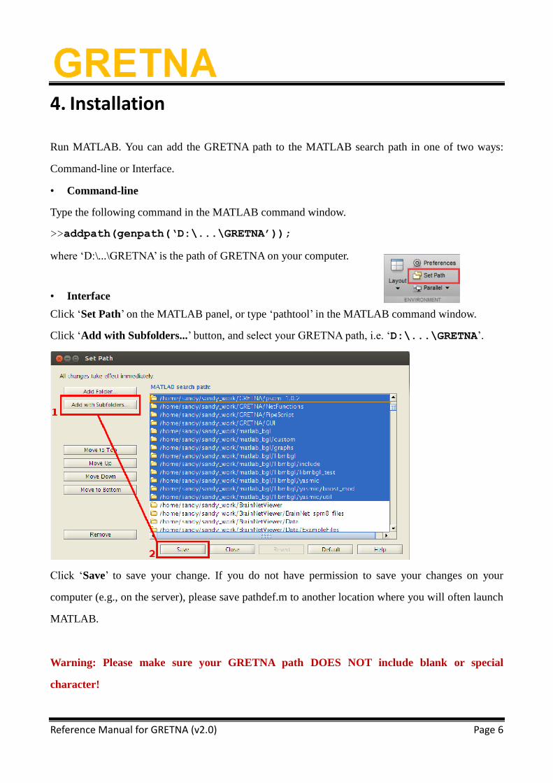
• Interface
Click ‘Set Path’ on the MATLAB panel, or type ‘pathtool’ in the MATLAB command window.
Click ‘Add with Subfolders...’ button, and select your GRETNA path, i.e. ‘D:\...\GRETNA’.
Click ‘Save’ to save your change. If you do not have permission to save your changes on your
computer (e.g., on the server), please save pathdef.m to another location where you will often launch
MATLAB.
Warning: Please make sure your GRETNA path DOES NOT include blank or special
character!
Page 7
Reference Manual for GRETNA (v2.0) Page 7
Type ‘gretna’ to start analyzing on your data! Be sure to type in lowercase characters.
>>gretna
In this version, GRETNA is divided into five sections:
• FC Matrix Construction: This section allows researchers to 1) perform R-fMRI data
preprocessing, including volume removal, slice timing, realignment, spatial normalization, spatial
smoothing, detrend, temporal filtering and removal of confounding variables by regression; and 2)
construct static or dynamic region of interest (ROI)-based functional connectivity matrices.
• Network Analysis: This section allows researchers to 1) convert individual connectivity matrices
into a series of sparse networks according to the pre-assigned parameters of the network type
(binary or weighted), network connectivity member (absolute, positive or negative), threshold
type (connectivity strength or sparsity), and threshold range; 2) generate benchmark random
networks that match real brain networks with respect to the number of nodes and edges and
degree distribution; and 3) calculate graph-based global and nodal network metrics.
• Metric comparison: This section allows researchers to 1) perform statistical inferencing on
global, nodal and connectional network parameters; 2) estimate network-behavior relationships;
and 3) generate group-level network.
• Metric plotting: This section allows researchers to plot bar charts, dot graphs, violin graphs and
shape graphs of the results obtained from metric comparison.
Page 8
Reference Manual for GRETNA (v2.0) Page 8
• GANNM: This section allows researchers to perform nonparametric statistical inferencing on
structural network using permutations.
5. Network Construction
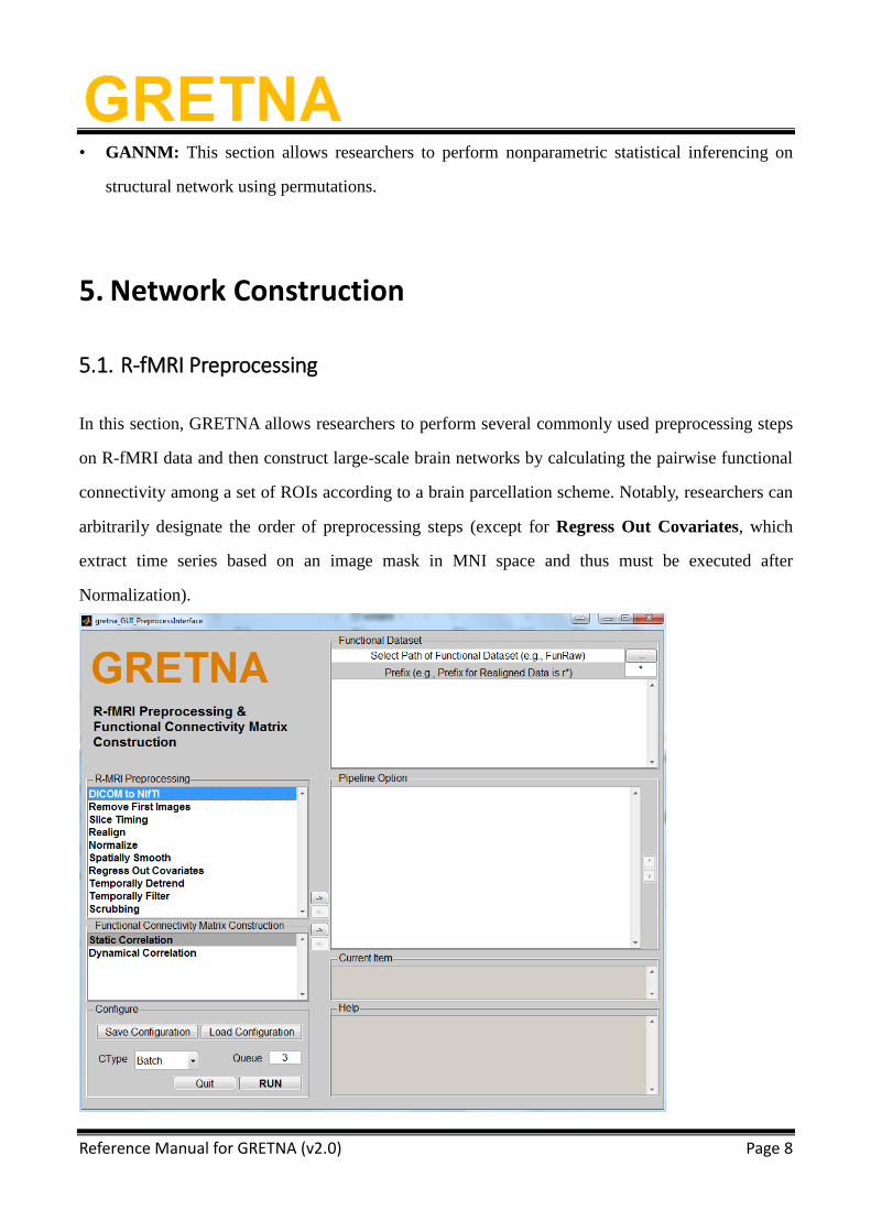
5.1. R-fMRI Preprocessing
In this section, GRETNA allows researchers to perform several commonly used preprocessing steps
on R-fMRI data and then construct large-scale brain networks by calculating the pairwise functional
connectivity among a set of ROIs according to a brain parcellation scheme. Notably, researchers can
arbitrarily designate the order of preprocessing steps (except for Regress Out Covariates, which
extract time series based on an image mask in MNI space and thus must be executed after
Normalization).
Page 9
Reference Manual for GRETNA (v2.0) Page 9
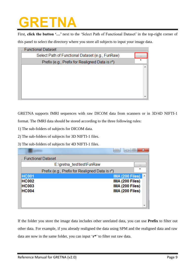
First, click the button ‘…’ next to the ‘Select Path of Functional Dataset’ in the top-right corner of
this panel to select the directory where you store all subjects to input your image data.
GRETNA supports fMRI sequences with raw DICOM data from scanners or in 3D/4D NIFTI-1
format. The fMRI data should be stored according to the three following rules:
1) The sub-folders of subjects for DICOM data.
2) The sub-folders of subjects for 3D NIFTI-1 files.
3) The sub-folders of subjects for 4D NIFTI-1 files.
If the folder you store the image data includes other unrelated data, you can use Prefix to filter out
other data. For example, if you already realigned the data using SPM and the realigned data and raw
data are now in the same folder, you can input ‘r*’ to filter out raw data.
Page 10
Reference Manual for GRETNA (v2.0) Page 10
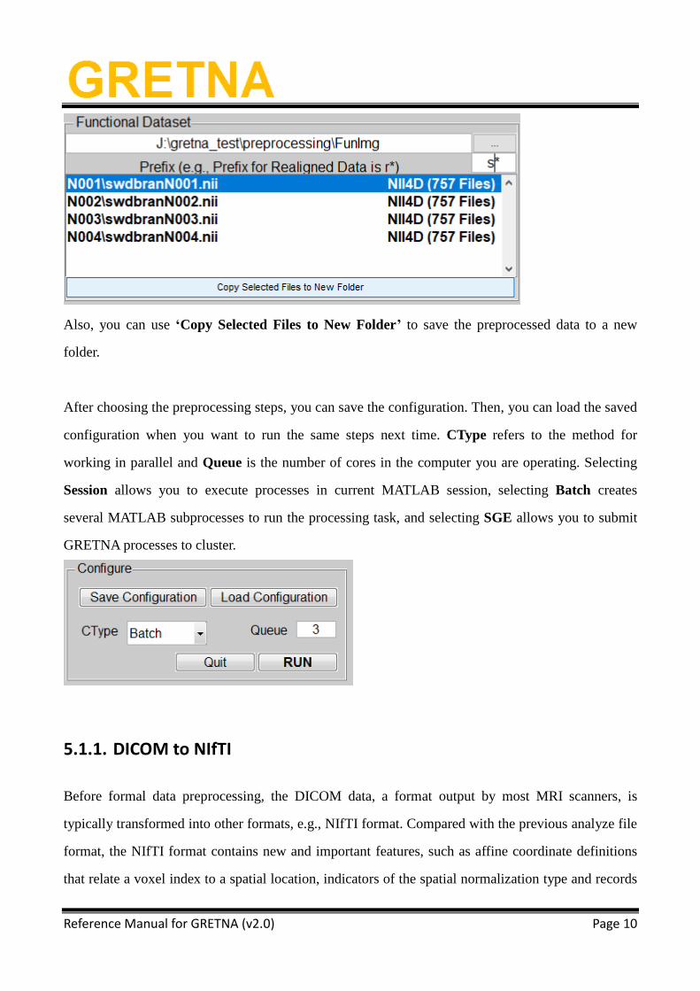
Also, you can use ‘Copy Selected Files to New Folder’ to save the preprocessed data to a new
folder.
After choosing the preprocessing steps, you can save the configuration. Then, you can load the saved
configuration when you want to run the same steps next time. CType refers to the method for
working in parallel and Queue is the number of cores in the computer you are operating. Selecting
Session allows you to execute processes in current MATLAB session, selecting Batch creates
several MATLAB subprocesses to run the processing task, and selecting SGE allows you to submit
GRETNA processes to cluster.
5.1.1. DICOM to NIfTI
Before formal data preprocessing, the DICOM data, a format output by most MRI scanners, is
typically transformed into other formats, e.g., NIfTI format. Compared with the previous analyze file
format, the NIfTI format contains new and important features, such as affine coordinate definitions
that relate a voxel index to a spatial location, indicators of the spatial normalization type and records
Page 11
Reference Manual for GRETNA (v2.0) Page 11
of the spatio-temporal slice ordering. This conversion is achieved in GRETNA by calling dcm2nii in
the MRIcroN software (http://www.mccauslandcenter.sc.edu/mricro/mricron/).
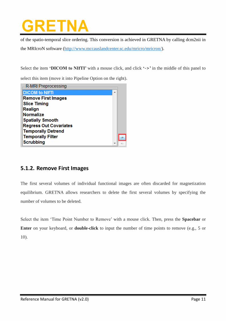
Select the item ‘DICOM to NIfTI’ with a mouse click, and click ‘->’ in the middle of this panel to
select this item (move it into Pipeline Option on the right).
5.1.2. Remove First Images
The first several volumes of individual functional images are often discarded for magnetization
equilibrium. GRETNA allows researchers to delete the first several volumes by specifying the
number of volumes to be deleted.
Select the item ‘Time Point Number to Remove’ with a mouse click. Then, press the Spacebar or
Enter on your keyboard, or double-click to input the number of time points to remove (e.g., 5 or
10).
Page 12
Reference Manual for GRETNA (v2.0) Page 12
5.1.3. Slice Timing
R-fMRI datasets are usually acquired using repeated 2D imaging methods, which leads to temporal
offsets between slices. Slice timing correction is performed in GRETNA by calling the
corresponding SPM8/SPM12 functions. It should be noted that, for a longer repeat time (e.g., > 3 s),
within which a whole brain volume is acquired, it is advised to omit the slice time correction step
because interpolation in this case becomes less accurate.
Set the following parameters according to your data.
Page 13
Reference Manual for GRETNA (v2.0) Page 13
• TR (s): The time of repeat of an fMRI signal.
• Slice Order: The sequence of slices. We have provided six different options: alternating in the
plus direction starting with odd-numbered slices (i.e., 1 3 5...2 4 6…), alternating in the plus
direction starting with even-numbered slices (i.e., 2 4 6…1 3 5), alternating in the minus
direction starting with odd-numbered slices (i.e., 33 31 29...32 30 28…), alternating in the plus
direction starting with even-numbered slices (i.e., 32 30 28…33 31 29…), running sequentially
in the plus direction (i.e., 1 2 3…31 32 33), and running sequentially in the minus direction (i.e.,
33 32 31…3 2 1).
• Reference Slice: The slice used as a reference to perform the timing correction. You can choose
the first slice, middle slice (middle of time), or last slice as a reference. The default option is
middle slice.
When you add several preprocessing steps into the pipeline option, you can use the buttons located
on the right to adjust the sequence of the preprocessing steps for fMRI data.
5.1.4. Realign
During an MR scan, participants inevitably undergo various degrees of head movement, even when
foam pads are used. The movements break the spatial correspondence of the brain across volumes.
Page 14
Reference Manual for GRETNA (v2.0) Page 14
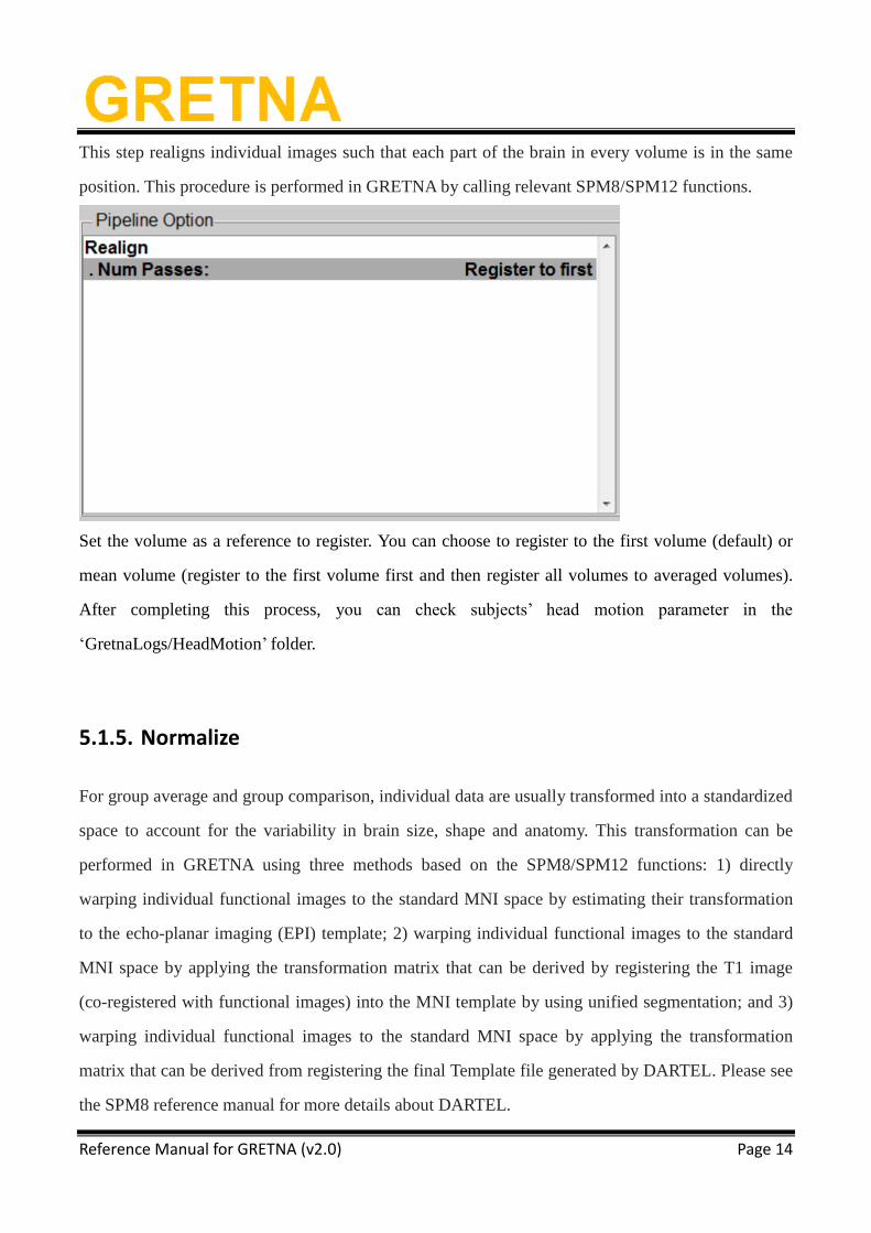
This step realigns individual images such that each part of the brain in every volume is in the same
position. This procedure is performed in GRETNA by calling relevant SPM8/SPM12 functions.
Set the volume as a reference to register. You can choose to register to the first volume (default) or
mean volume (register to the first volume first and then register all volumes to averaged volumes).
After completing this process, you can check subjects’ head motion parameter in the
‘GretnaLogs/HeadMotion’ folder.
5.1.5. Normalize
For group average and group comparison, individual data are usually transformed into a standardized
space to account for the variability in brain size, shape and anatomy. This transformation can be
performed in GRETNA using three methods based on the SPM8/SPM12 functions: 1) directly
warping individual functional images to the standard MNI space by estimating their transformation
to the echo-planar imaging (EPI) template; 2) warping individual functional images to the standard
MNI space by applying the transformation matrix that can be derived by registering the T1 image
(co-registered with functional images) into the MNI template by using unified segmentation; and 3)
warping individual functional images to the standard MNI space by applying the transformation
matrix that can be derived from registering the final Template file generated by DARTEL. Please see
the SPM8 reference manual for more details about DARTEL.
Page 15
Reference Manual for GRETNA (v2.0) Page 15
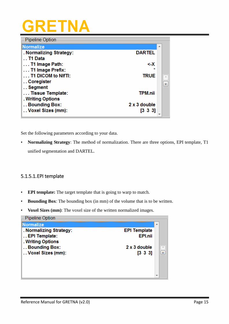
Set the following parameters according to your data.
• Normalizing Strategy: The method of normalization. There are three options, EPI template, T1
unified segmentation and DARTEL.
5.1.5.1. EPI template
• EPI template: The target template that is going to warp to match.
• Bounding Box: The bounding box (in mm) of the volume that is to be written.
• Voxel Sizes (mm): The voxel size of the written normalized images.
Page 16
Reference Manual for GRETNA (v2.0) Page 16
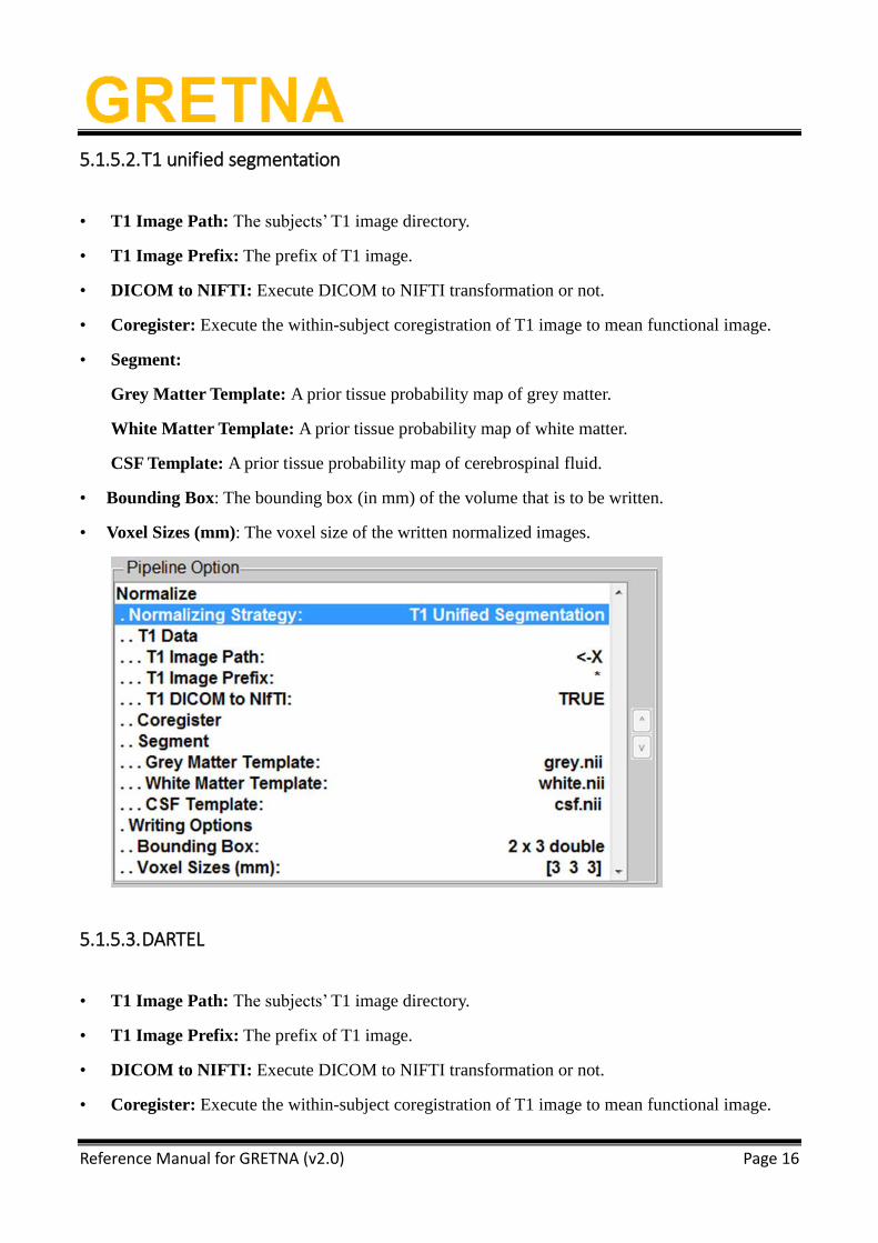
5.1.5.2. T1 unified segmentation
• T1 Image Path: The subjects’ T1 image directory.
• T1 Image Prefix: The prefix of T1 image.
• DICOM to NIFTI: Execute DICOM to NIFTI transformation or not.
• Coregister: Execute the within-subject coregistration of T1 image to mean functional image.
• Segment:
Grey Matter Template: A prior tissue probability map of grey matter.
White Matter Template: A prior tissue probability map of white matter.
CSF Template: A prior tissue probability map of cerebrospinal fluid.
• Bounding Box: The bounding box (in mm) of the volume that is to be written.
• Voxel Sizes (mm): The voxel size of the written normalized images.
5.1.5.3. DARTEL
• T1 Image Path: The subjects’ T1 image directory.
• T1 Image Prefix: The prefix of T1 image.
• DICOM to NIFTI: Execute DICOM to NIFTI transformation or not.
• Coregister: Execute the within-subject coregistration of T1 image to mean functional image.
Page 17
Reference Manual for GRETNA (v2.0) Page 17
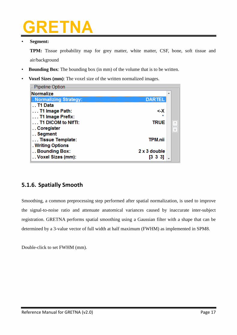
• Segment:
TPM: Tissue probability map for grey matter, white matter, CSF, bone, soft tissue and
air/background
• Bounding Box: The bounding box (in mm) of the volume that is to be written.
• Voxel Sizes (mm): The voxel size of the written normalized images.
5.1.6. Spatially Smooth
Smoothing, a common preprocessing step performed after spatial normalization, is used to improve
the signal-to-noise ratio and attenuate anatomical variances caused by inaccurate inter-subject
registration. GRETNA performs spatial smoothing using a Gaussian filter with a shape that can be
determined by a 3-value vector of full width at half maximum (FWHM) as implemented in SPM8.
Double-click to set FWHM (mm).
Page 18
Reference Manual for GRETNA (v2.0) Page 18
5.1.7. Regress Out Covariates
For R-fMRI datasets, several nuisance signals are typically removed from each voxel’s time series to
reduce the effects of non-neuronal fluctuations, including head motion profiles, the cerebrospinal
fluid signal, the white matter signals and/or the global signal. In GRETNA, researchers can assign
any combination of these variables to be variables of no interest, which will be regressed out. The
global signal, CSF signal and white matter signal are calculated by using the whole brain, cerebral
spinal fluid and WM masks in the standard MNI space from the REST toolbox (default). Set the
following parameters according to your research purposes.
• Global Signal: Regress out global signal or not. You can also change the mask of the whole
brain if necessary.
• White Matter Signal: Regress out white matter signal or not. You can also change the mask of
the white matter if necessary.
• CSF Signal: Regress out cerebrospinal fluid signal or not. You can also change the mask of
cerebrospinal fluid if necessary.
• Head Motion: Regress out head motion parameters or not. Options include the original 6
parameters, the original and relative 12-parameters and the Friston 24 parameters.
Page 19
Reference Manual for GRETNA (v2.0) Page 19
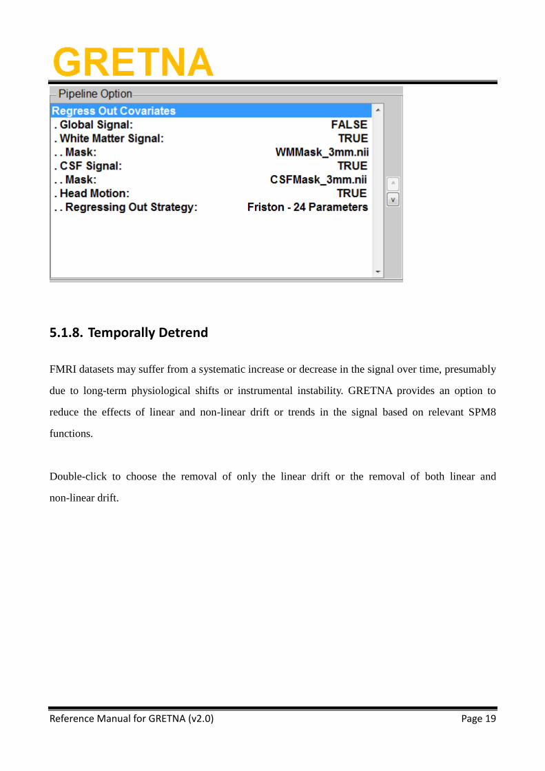
5.1.8. Temporally Detrend
FMRI datasets may suffer from a systematic increase or decrease in the signal over time, presumably
due to long-term physiological shifts or instrumental instability. GRETNA provides an option to
reduce the effects of linear and non-linear drift or trends in the signal based on relevant SPM8
functions.
Double-click to choose the removal of only the linear drift or the removal of both linear and
non-linear drift.
Page 20
Reference Manual for GRETNA (v2.0) Page 20
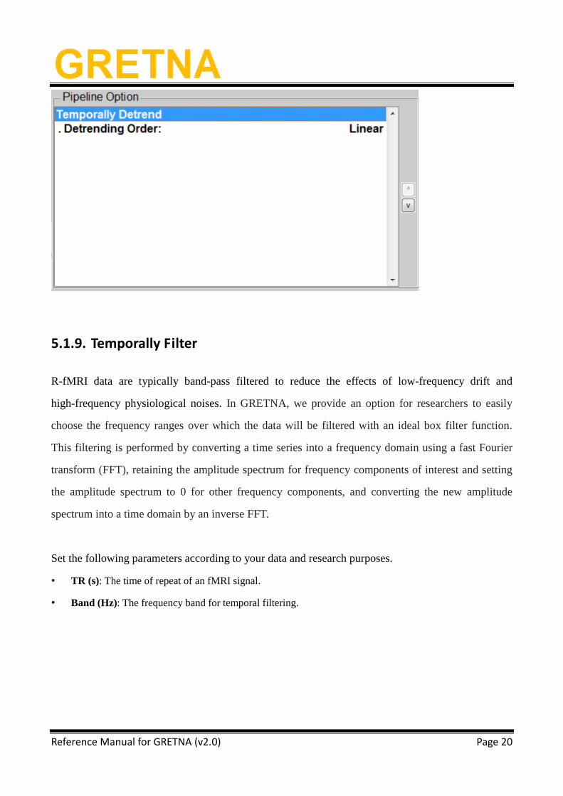
5.1.9. Temporally Filter
R-fMRI data are typically band-pass filtered to reduce the effects of low-frequency drift and
high-frequency physiological noises. In GRETNA, we provide an option for researchers to easily
choose the frequency ranges over which the data will be filtered with an ideal box filter function.
This filtering is performed by converting a time series into a frequency domain using a fast Fourier
transform (FFT), retaining the amplitude spectrum for frequency components of interest and setting
the amplitude spectrum to 0 for other frequency components, and converting the new amplitude
spectrum into a time domain by an inverse FFT.
Set the following parameters according to your data and research purposes.
• TR (s): The time of repeat of an fMRI signal.
• Band (Hz): The frequency band for temporal filtering.
Page 21
Reference Manual for GRETNA (v2.0) Page 21
5.1.10. Scrubbing
Scrubbing is a quality control process used to reduce the effects of head motion on R-fMRI data.
This process uses realignment parameters to identify frames that may be of poor quality and take
apply a certain strategy to these frames (e.g., remove or interpolate).
Set the following parameters.
• Interpolation Strategy: The strategy adopted to process frames of poor quality. You can choose
to remove these flames or replace these flames with the nearest or linear interpolation.
• FD Threshold: The threshold of frame-wise displacement (FD) above which the frame would
be considered to be of with poor quality.
Page 22
Reference Manual for GRETNA (v2.0) Page 22
• Previous Time Point Number: The number of time point before the frames of poor quality that
would be removed or replaced.
• Subsequent Time Point Number: The number of time point after the frames of poor quality
that would be removed or replaced.
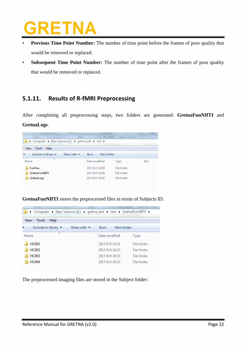
5.1.11. Results of R-fMRI Preprocessing
After completing all preprocessing steps, two folders are generated: GretnaFunNIfTI and
GretnaLogs.
GretnaFunNIfTI stores the preprocessed files in terms of Subjects ID.
The preprocessed imaging files are stored in the Subject folder:
Page 23
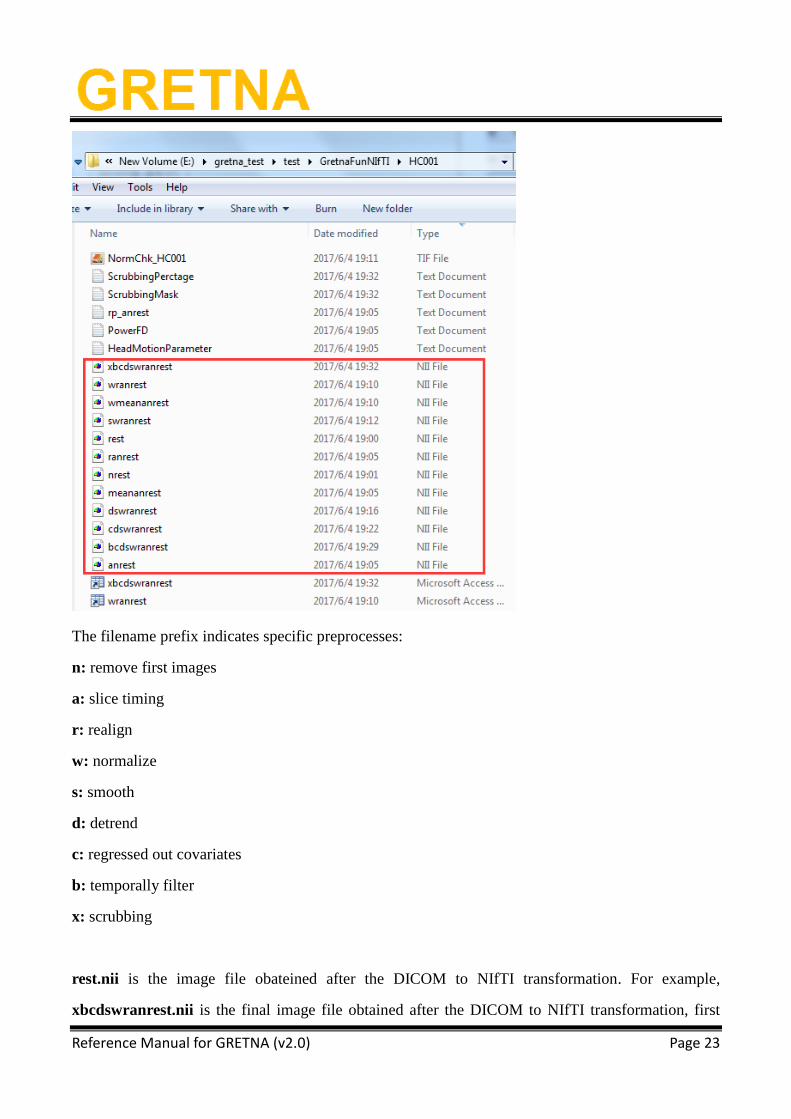
Reference Manual for GRETNA (v2.0) Page 23
The filename prefix indicates specific preprocesses:
n: remove first images
a: slice timing
r: realign
w: normalize
s: smooth
d: detrend
c: regressed out covariates
b: temporally filter
x: scrubbing
rest.nii is the image file obateined after the DICOM to NIfTI transformation. For example,
xbcdswranrest.nii is the final image file obtained after the DICOM to NIfTI transformation, first
Page 24
Reference Manual for GRETNA (v2.0) Page 24
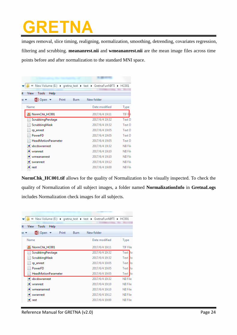
images removal, slice timing, realigning, normalization, smoothing, detrending, covariates regression,
filtering and scrubbing. meananrest.nii and wmeananrest.nii are the mean image files across time
points before and after normalization to the standard MNI space.
NormChk_HC001.tif allows for the quality of Normalization to be visually inspected. To check the
quality of Normalization of all subject images, a folder named NormalizationInfo in GretnaLogs
includes Normalization check images for all subjects.
Page 25
Reference Manual for GRETNA (v2.0) Page 25
In addition, several head motion parameter files are also generated in this folder.
HeadMotionParameter.txt stores six head motion parameters, including three translations and three
rotations parameters. The Power flame-wise distance (FD) for each time point is also calculated in
PowerFD.txt. The percentage of flames above a given threshold (e.g. FD>0.05) in scrubbing is
calculated in ScrubbingPerctage.txt. PowerFD files for all subjects can be found in folder ‘…\
GretnaLogs\HeadMotionInfo\PowerFD’.
5.2. Functional Connectivity Matrix Construction
This option is used to construct individual interregional functional connectivity matrices in two
major steps: region parcellation (i.e., network node definition) and functional connectivity estimation
(i.e., network edge definition). GRETNA provides options for several different parcellation schemes,
including the structurally defined Anatomical Automatic Labeling atlas (AAL-90, AAL116) and
Harvard-Oxford atlas (HOA-112) and the functionally defined Dos-160, Crad-200, Power-264 and
Fair-34. Additionally, GRETNA contains parcellation schemes defined by randomly parceling the
brain into 625 (random-625) or 1024 (random-1024) ROIs. Once a parcellation scheme is chosen, the
mean time series will be extracted from each parcellation unit, and pairwise functional connectivity
is then estimated among the time series by calculating linear Pearson correlation coefficients. This
procedure will generate an N × N correlation matrix for each participant, where N is the number of
regions included in the selected brain parcellation. It should be noted that this section also allows
researchers to construct a dynamic correlation matrix based on a sliding time-window approach.
Page 26
Reference Manual for GRETNA (v2.0) Page 26
5.2.1. Static Correlation
Set the following parameters to construct static functional connectivity matrices for each subject in
your data.
• Atlas: The brain parcellation for network node definition.
• Fisher’s Z Transform: Perform the Fisher’s r-to-z transformation to improve the normality of
the correlations or not.
5.2.2. Dynamical Correlation
Page 27
Reference Manual for GRETNA (v2.0) Page 27
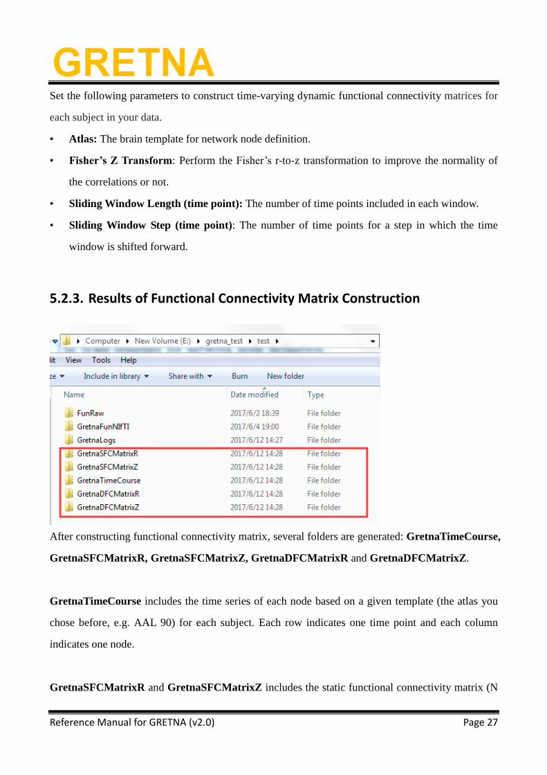
Set the following parameters to construct time-varying dynamic functional connectivity matrices for
each subject in your data.
• Atlas: The brain template for network node definition.
• Fisher’s Z Transform: Perform the Fisher’s r-to-z transformation to improve the normality of
the correlations or not.
• Sliding Window Length (time point): The number of time points included in each window.
• Sliding Window Step (time point): The number of time points for a step in which the time
window is shifted forward.
5.2.3. Results of Functional Connectivity Matrix Construction
After constructing functional connectivity matrix, several folders are generated: GretnaTimeCourse,
GretnaSFCMatrixR, GretnaSFCMatrixZ, GretnaDFCMatrixR and GretnaDFCMatrixZ.
GretnaTimeCourse includes the time series of each node based on a given template (the atlas you
chose before, e.g. AAL 90) for each subject. Each row indicates one time point and each column
indicates one node.
GretnaSFCMatrixR and GretnaSFCMatrixZ includes the static functional connectivity matrix (N
Page 28
Reference Manual for GRETNA (v2.0) Page 28
× N, N = number of nodes) for all subjects before and after Fisher z transformation.
GretnaDFCMatrixR and GretnaDFCMatrixZ includes the dynamic functional connectivity
matrix (N × N × T, N = number of nodes and T = number of time windows) for all subjects before
and after Fisher z transformation.
6. Network Analysis
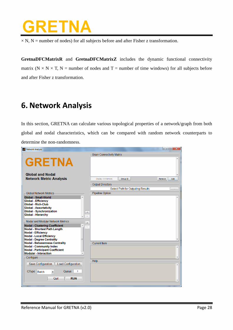
In this section, GRETNA can calculate various topological properties of a network/graph from both
global and nodal characteristics, which can be compared with random network counterparts to
determine the non-randomness.
Page 29
Reference Manual for GRETNA (v2.0) Page 29
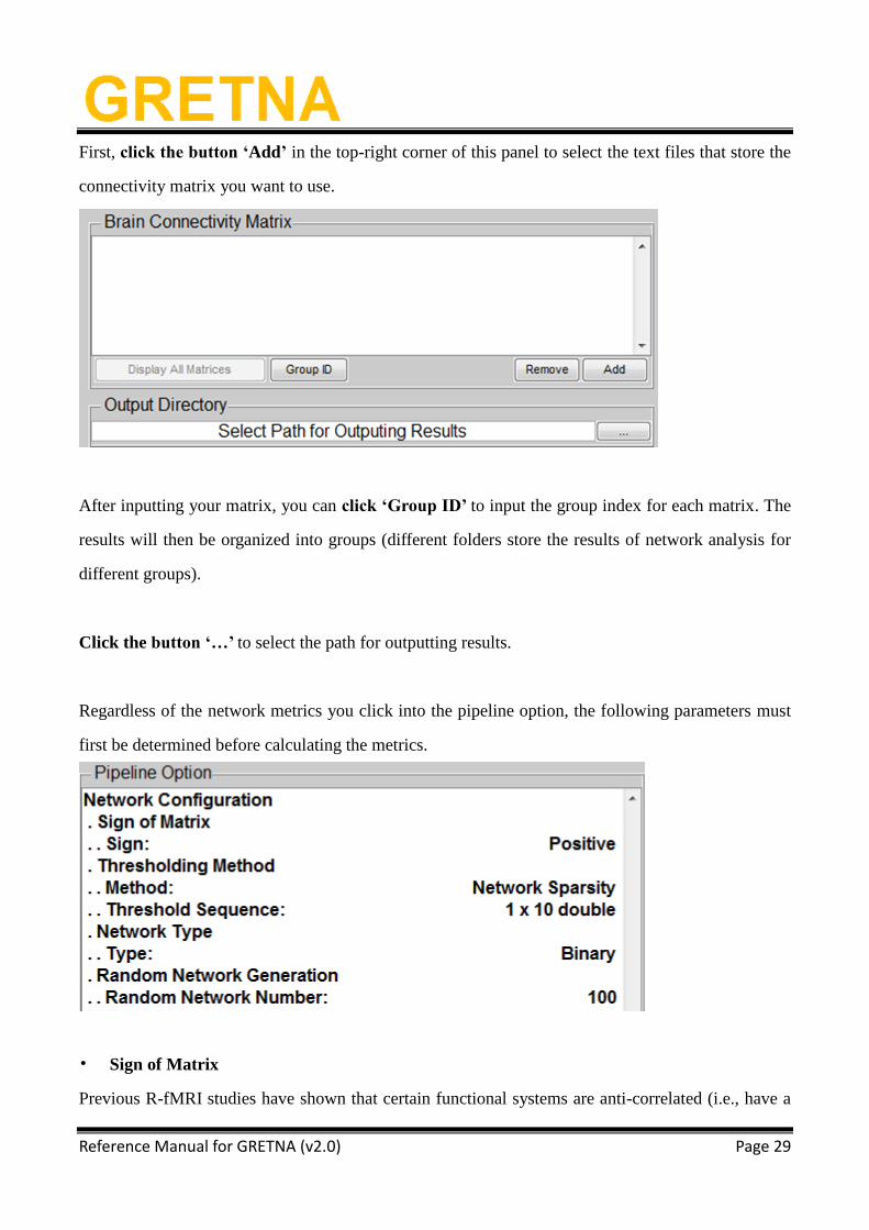
First, click the button ‘Add’ in the top-right corner of this panel to select the text files that store the
connectivity matrix you want to use.
After inputting your matrix, you can click ‘Group ID’ to input the group index for each matrix. The
results will then be organized into groups (different folders store the results of network analysis for
different groups).
Click the button ‘…’ to select the path for outputting results.
Regardless of the network metrics you click into the pipeline option, the following parameters must
first be determined before calculating the metrics.
• Sign of Matrix
Previous R-fMRI studies have shown that certain functional systems are anti-correlated (i.e., have a
Page 30
Reference Manual for GRETNA (v2.0) Page 30
negative correlation) in their spontaneous brain activity. However, negative correlations may also be
introduced by global signal removal, a preprocessing step that is currently controversial. For network
topology, negative correlations may have detrimental effects on TRT reliability and exhibit
organizations different from positive correlations. Accordingly, GRETNA provides options for
researchers to determine network connectivity members, based on which subsequent graph analyses
are implemented: positive (composed of only positive correlations), negative (composed of only
absolute values of negative correlations) or absolute (composed of both positive correlations and the
absolute values of the negative correlations).
• Thresholding Method
Prior to topological characterization, a thresholding procedure is typically applied to exclude the
confounding effects of spurious relationships in interregional connectivity matrices. Two
thresholding strategies are provided in GRETNA: the ‘Network Sparsity’ and ‘Value of Matrix
Element’. Specifically, for ‘Network Sparsity’, the threshold value is defined as the ratio of the
number of actual edges divided by the maximum possible number of edges in a network. For
networks with the same number of nodes, the sparsity threshold ensures the same number of edges
for each network by applying a subject-specific connectivity strength threshold and therefore
allowing for an examination of relative network organization. For ‘Value of Matrix Element’,
researchers can define a threshold value such that network connections with weights greater than the
given threshold are retained and others are ignored (i.e., set to 0). This connectivity strength
threshold method allows for the examination of absolute network organization. Note that the same
connectivity strength threshold usually leads to a different number of edges in the resultant networks,
which could confound between-group comparisons in network topology. These two thresholding
strategies are complementary and together provide a comprehensive method for testing network
organization. Finally, given the absence of a definitive method for selecting a single threshold,
researchers can input a range of continuous threshold values to study network properties in
GRETNA. Double-click ‘Threshold Sequence’ to set a range of continuous threshold values.
• Network Type
Page 31
Reference Manual for GRETNA (v2.0) Page 31
Networks can be binarized or weighted depending on whether connectivity strength is considered.
Previous brain network studies have mainly focused on binary networks because of the reduction in
computational complexity and clarity of network metric definitions. Notably, binary networks
neglect the strength of connections above the threshold and therefore fail to identify subtle network
organizations. In GRETNA, all network analyses can be conducted for both binary and weighted
networks.
• Random Networks
Brain networks are typically compared with random networks to test whether they are configured
with significantly non-random topology. In GRETNA, random networks are generated by a Markov
wiring algorithm [Maslov and Sneppen, 2002], which preserves the same number of nodes and edges
and the same degree distribution as real brain networks.
6.1. Global Network Metrics
GRETNA can calculate several widely used network metrics in brain network studies for both binary
and weighted networks. Generally, these measures can be categorized into global and nodal metrics.
Global metrics include small-world parameters of the clustering coefficient and characteristic path
length, local efficiency and global efficiency, modularity, assortativity, synchronization and hierarchy.
For the formula, usage and interpretation of these measures, see [Rubinov and Sporns, 2010] and
[Wang et al., 2011]. Finally, GRETNA can also calculate the area under the curve (AUC) for each
network measure to provide a scalar that does not depend on a specific threshold selection. It should
be noted that this module can perform topological analysis of brain networks, independent of
imaging modality and species. For example, the structural brain connectivity matrices in humans or
macaques that are obtained from the PANDA toolbox [Cui et al., 2013] or the CoCoMac database
can be entered into this module for graph analysis.
Page 32
Reference Manual for GRETNA (v2.0) Page 32
6.1.1. Small-World
Small-world networks have a shorter characteristic path length than regular networks (high clustering
and long path lengths) but greater local interconnectivity than random networks (low clustering
coefficient and short path lengths). The small-world metric supports both specialized/modularized
and integrated/distributed information processing and maximizes the efficiency of information
transfer at a relatively low wiring cost.
6.1.2. Efficiency
Global efficiency measures the global efficiency of parallel information transfer in a network. The
local efficiency of the network measures how efficient communication is among the first neighbors
of a given node when it is removed.
6.1.3. Rich-Club
Rich-club architecture is a nontrivial topological property of a brain network, indicating that the hub
nodes are more densely connected among themselves than non-hub nodes and thus form a highly
interconnected club.
Page 33
Reference Manual for GRETNA (v2.0) Page 33
6.1.4. Assortativity
Assortativity reflects the tendency of nodes to link those nodes with similar numbers of edges.
6.1.5. Synchronization
Synchronization measures how likely it is that all nodes fluctuate in the same wave pattern.
6.1.6. Hierarchy
The hierarchy coefficient is used to identify the presence of a hierarchical organization in a network
[Ravasz and Barabási, 2003].
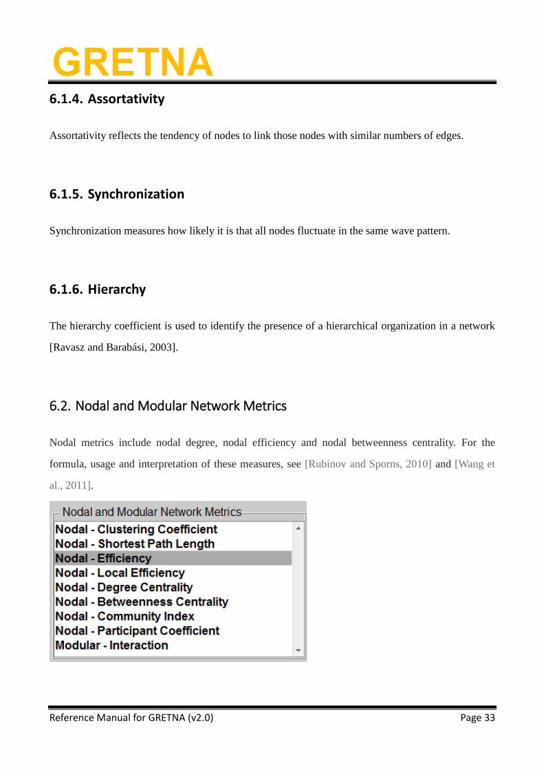
6.2. Nodal and Modular Network Metrics
Nodal metrics include nodal degree, nodal efficiency and nodal betweenness centrality. For the
formula, usage and interpretation of these measures, see [Rubinov and Sporns, 2010] and [Wang et
al., 2011].
Page 34
Reference Manual for GRETNA (v2.0) Page 34
6.2.1. Clustering Coefficient
The clustering coefficient of a given node measures the likelihood its neighborhoods are connected
to each other.
6.2.2. Shortest Path Length
The shortest path length of a given node quantifies the mean distance or routing efficiency between
this node and all the other nodes in the network.
6.2.3. Efficiency
The nodal efficiency for a given node characterizes the efficiency of parallel information transfer of
that node in the network.
6.2.4. Local Efficiency
The local efficiency for a given node measures how efficient the communication is among the first
neighbors of this node when it is removed.
6.2.5. Degree Centrality
The nodal degree for a given node reflects its information communication ability in the functional
network.
Page 35
Reference Manual for GRETNA (v2.0) Page 35
6.2.6. Betweenness Centrality
The nodal betweenness for a given node characterizes its effect on information flow between other
nodes.
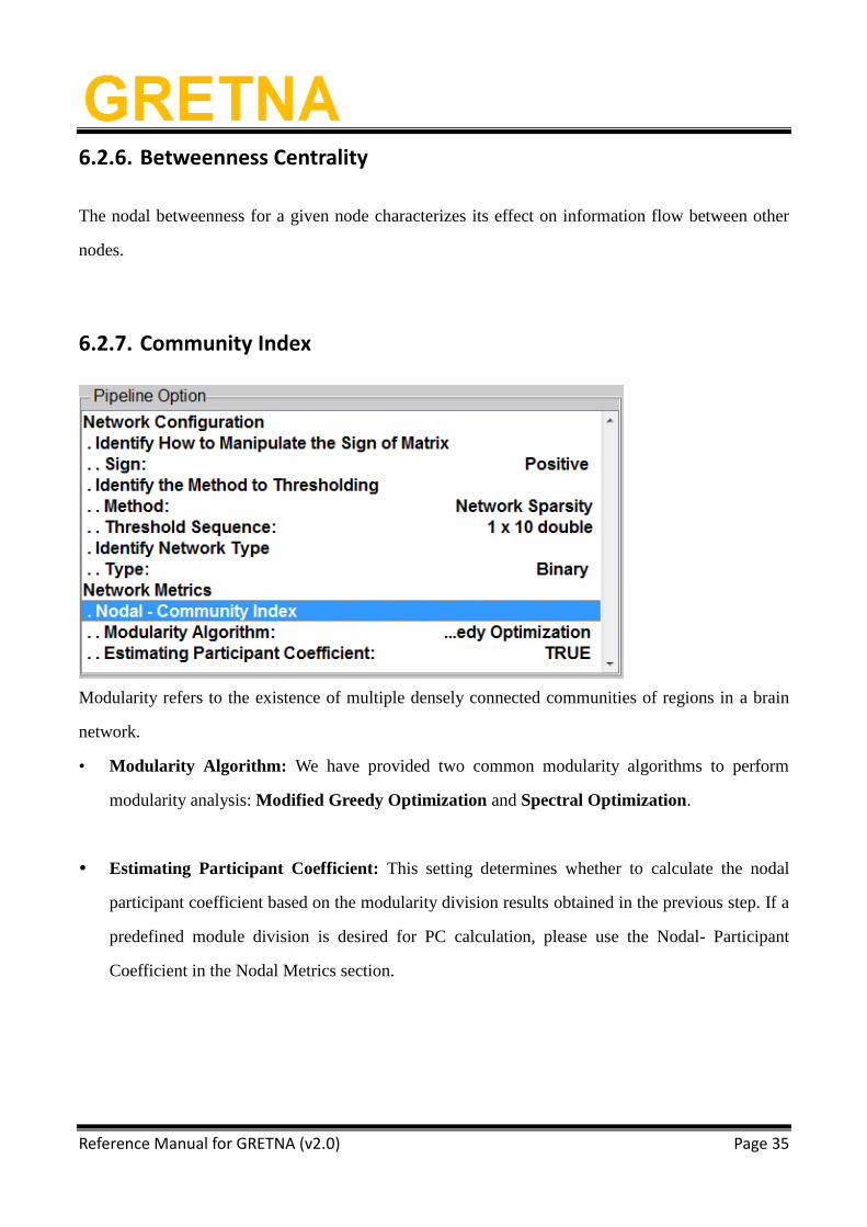
6.2.7. Community Index
Modularity refers to the existence of multiple densely connected communities of regions in a brain
network.
• Modularity Algorithm: We have provided two common modularity algorithms to perform
modularity analysis: Modified Greedy Optimization and Spectral Optimization.
Estimating Participant Coefficient: This setting determines whether to calculate the nodal
participant coefficient based on the modularity division results obtained in the previous step. If a
predefined module division is desired for PC calculation, please use the Nodal- Participant
Coefficient in the Nodal Metrics section.
Page 36
Reference Manual for GRETNA (v2.0) Page 36
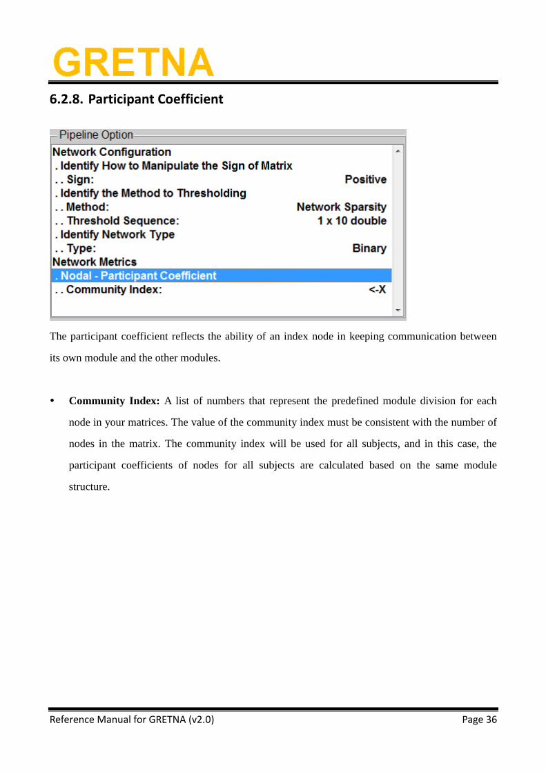
6.2.8. Participant Coefficient
The participant coefficient reflects the ability of an index node in keeping communication between
its own module and the other modules.
Community Index: A list of numbers that represent the predefined module division for each
node in your matrices. The value of the community index must be consistent with the number of
nodes in the matrix. The community index will be used for all subjects, and in this case, the
participant coefficients of nodes for all subjects are calculated based on the same module
structure.
Page 37
Reference Manual for GRETNA (v2.0) Page 37
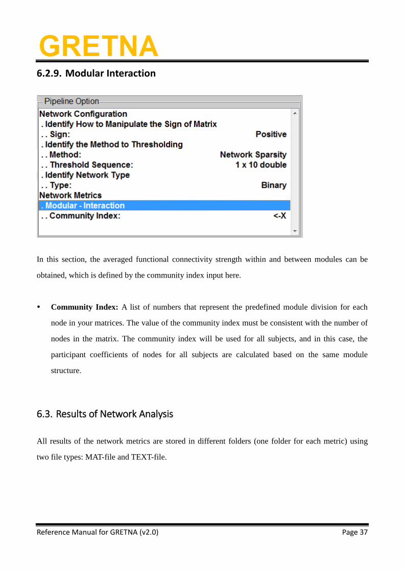
6.2.9. Modular Interaction
In this section, the averaged functional connectivity strength within and between modules can be
obtained, which is defined by the community index input here.
Community Index: A list of numbers that represent the predefined module division for each
node in your matrices. The value of the community index must be consistent with the number of
nodes in the matrix. The community index will be used for all subjects, and in this case, the
participant coefficients of nodes for all subjects are calculated based on the same module
structure.
6.3. Results of Network Analysis
All results of the network metrics are stored in different folders (one folder for each metric) using
two file types: MAT-file and TEXT-file.
Page 38
Reference Manual for GRETNA (v2.0) Page 38
6.3.1. Global Network Metrics
Small-World
aCp: The AUC (area under curve) of the clustering coefficient of a network for each subject.
aGamma: The AUC of the Gamma of a network for each subject.
aLambda: The AUC of the Lambda of a network for each subject.
aLp: The AUC of the shortest path length of a network for each subject.
aSigma: The AUC of the Sigma of a network for each subject.
Cp_All_Thres: Clustering coefficient of a network at each threshold for each subject. Each row
represents one subject, and each column represents one threshold.
Gamma_All_Thres: The Gamma of a network at each threshold for each subject.
Lambda_All_Thres: The Lambda of a network at each threshold for each subject.
Lp_All_Thres: The shortest path length of a network at each threshold for each subject.
Sigma_All_Thres: The Sigma of network at each threshold for each subject.
SmallWorld.mat includes all of these metrics and can loaded in MATLAB.
Page 39
Reference Manual for GRETNA (v2.0) Page 39
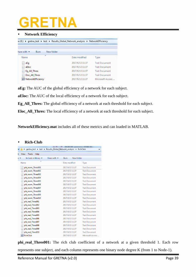
Network Efficiency
aEg: The AUC of the global efficiency of a network for each subject.
aEloc: The AUC of the local efficiency of a network for each subject.
Eg_All_Thres: The global efficiency of a network at each threshold for each subject.
Eloc_All_Thres: The local efficiency of a network at each threshold for each subject.
NetworkEfficiency.mat includes all of these metrics and can loaded in MATLAB.
Rich-Club
phi_real_Thres001: The rich club coefficient of a network at a given threshold 1. Each row
represents one subject, and each column represents one binary node degree K (from 1 to Node-1).
Page 40
Reference Manual for GRETNA (v2.0) Page 40
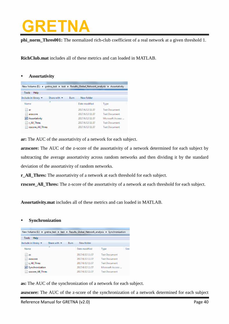
phi_norm_Thres001: The normalized rich-club coefficient of a real network at a given threshold 1.
RichClub.mat includes all of these metrics and can loaded in MATLAB.
Assortativity
ar: The AUC of the assortativity of a network for each subject.
arzscore: The AUC of the z-score of the assortativity of a network determined for each subject by
subtracting the average assortativity across random networks and then dividing it by the standard
deviation of the assortativity of random networks.
r_All_Thres: The assortativity of a network at each threshold for each subject.
rzscore_All_Thres: The z-score of the assortativity of a network at each threshold for each subject.
Assortativity.mat includes all of these metrics and can loaded in MATLAB.
Synchronization
as: The AUC of the synchronization of a network for each subject.
aszscore: The AUC of the z-score of the synchronization of a network determined for each subject
Page 41
Reference Manual for GRETNA (v2.0) Page 41
by subtracting the average synchronization across random networks and then dividing it by the
standard deviation of the synchronization of random networks.
s_All_Thres: The synchronization of a network at each threshold for each subject.
szscore_All_Thres: The z-score of the synchronization of a network at each threshold for each
subject.
Synchronization.mat includes all of these metrics and can loaded in MATLAB.
Hierarchy
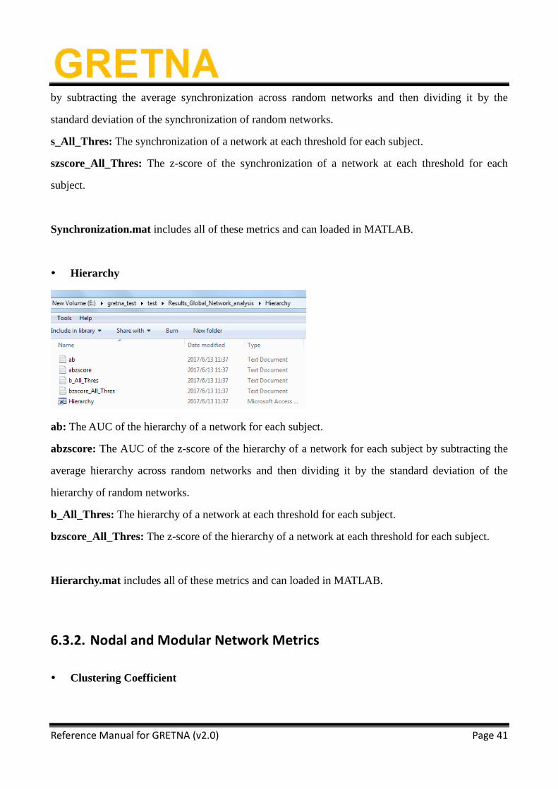
ab: The AUC of the hierarchy of a network for each subject.
abzscore: The AUC of the z-score of the hierarchy of a network for each subject by subtracting the
average hierarchy across random networks and then dividing it by the standard deviation of the
hierarchy of random networks.
b_All_Thres: The hierarchy of a network at each threshold for each subject.
bzscore_All_Thres: The z-score of the hierarchy of a network at each threshold for each subject.
Hierarchy.mat includes all of these metrics and can loaded in MATLAB.
6.3.2. Nodal and Modular Network Metrics
Clustering Coefficient
Page 42
Reference Manual for GRETNA (v2.0) Page 42
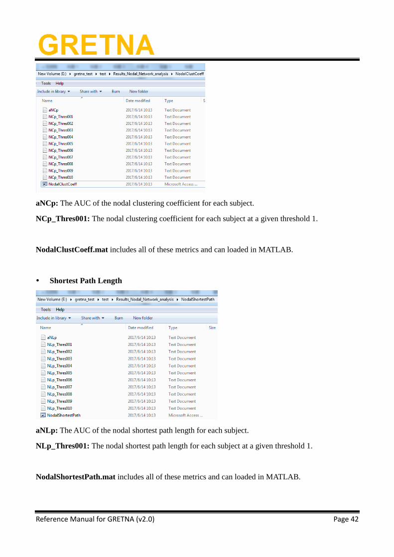
aNCp: The AUC of the nodal clustering coefficient for each subject.
NCp_Thres001: The nodal clustering coefficient for each subject at a given threshold 1.
NodalClustCoeff.mat includes all of these metrics and can loaded in MATLAB.
Shortest Path Length
aNLp: The AUC of the nodal shortest path length for each subject.
NLp_Thres001: The nodal shortest path length for each subject at a given threshold 1.
NodalShortestPath.mat includes all of these metrics and can loaded in MATLAB.
Page 43
Reference Manual for GRETNA (v2.0) Page 43
Efficiency
aNe: The AUC of the nodal efficiency for each subject.
Ne_Thres001: The nodal efficiency for each subject at a given threshold 1.
NodalEfficiency.mat includes all of these metrics and can loaded in MATLAB.
Local Efficiency
aNLe: The AUC of the nodal local efficiency for each subject.
NLe_Thres001: The nodal local efficiency for each subject at a given threshold 1.
NodalLocalEfficiency.mat includes all of these metrics and can loaded in MATLAB.
Page 44
Reference Manual for GRETNA (v2.0) Page 44
Degree Centrality
aDc: The AUC of the nodal degree centrality for each subject.
Dc_Thres001: The nodal degree centrality for each subject at a given threshold 1.
DegreeCentrality.mat includes all of these metrics and can loaded in MATLAB.
Betweenness Centrality
aBc: The AUC of the nodal betweenness for each subject.
Bc_Thres001: The nodal betweenness for each subject at a given threshold 1.
Page 45
Reference Manual for GRETNA (v2.0) Page 45
BetweennessCentrality.mat includes all of these metrics and can loaded in MATLAB.
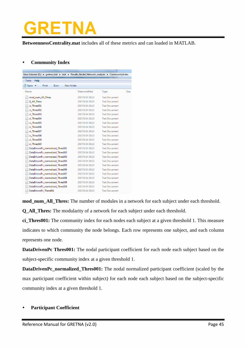
Community Index
mod_num_All_Thres: The number of modules in a network for each subject under each threshold.
Q_All_Thres: The modularity of a network for each subject under each threshold.
ci_Thres001: The community index for each nodes each subject at a given threshold 1. This measure
indicates to which community the node belongs. Each row represents one subject, and each column
represents one node.
DataDrivenPc Thres001: The nodal participant coefficient for each node each subject based on the
subject-specific community index at a given threshold 1.
DataDrivenPc_normalized_Thres001: The nodal normalized participant coefficient (scaled by the
max participant coefficient within subject) for each node each subject based on the subject-specific
community index at a given threshold 1.
Participant Coefficient
Page 46
Reference Manual for GRETNA (v2.0) Page 46
CustomPc_Thres001: The nodal participant coefficient for each node each subject based on the
same given community index at a given threshold 1.
CustomPc_normalized_Thres001: The nodal normalized participant coefficient (scaled by the max
participant coefficient within subject) for each node each subject based on the same given
community index at a given threshold 1.
ParticipantCoefficient.mat includes all of these metrics and can loaded in MATLAB.
Modular Interaction
SumEdgeNum_Within_Module01_All_Thres: The total number of edges within module 1 for
each subject based on the same given community index at all thresholds.
Page 47
Reference Manual for GRETNA (v2.0) Page 47
SumEdgeNum_Between_Module01_02_All_Thres: The total number of edges between module 1
and module 2 for each subject based on the same given community index at all thresholds.
ModularInteraction.mat includes all of these metrics and can loaded in MATLAB.
7. Metric Comparison
In this section, GRETNA allows researchers to perform statistical analysis on global, nodal and
connectional network measures.
7.1. Network and Node
For global and nodal network measures, GRETNA provides several popular parametric models,
including the one-sample t-test, two-sample t-test, paired t-test, one-way analysis of variance
(ANOVA) and repeated measurement ANOVA.
Page 48
Reference Manual for GRETNA (v2.0) Page 48
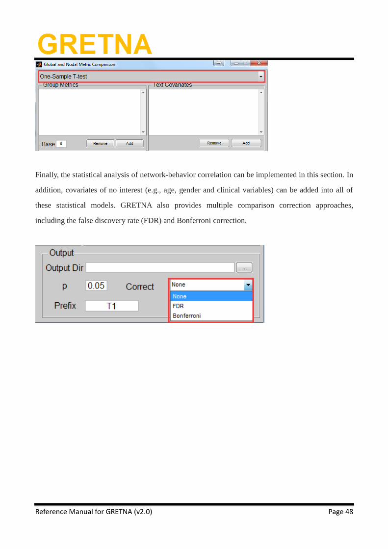
Finally, the statistical analysis of network-behavior correlation can be implemented in this section. In
addition, covariates of no interest (e.g., age, gender and clinical variables) can be added into all of
these statistical models. GRETNA also provides multiple comparison correction approaches,
including the false discovery rate (FDR) and Bonferroni correction.
Page 49
Reference Manual for GRETNA (v2.0) Page 49
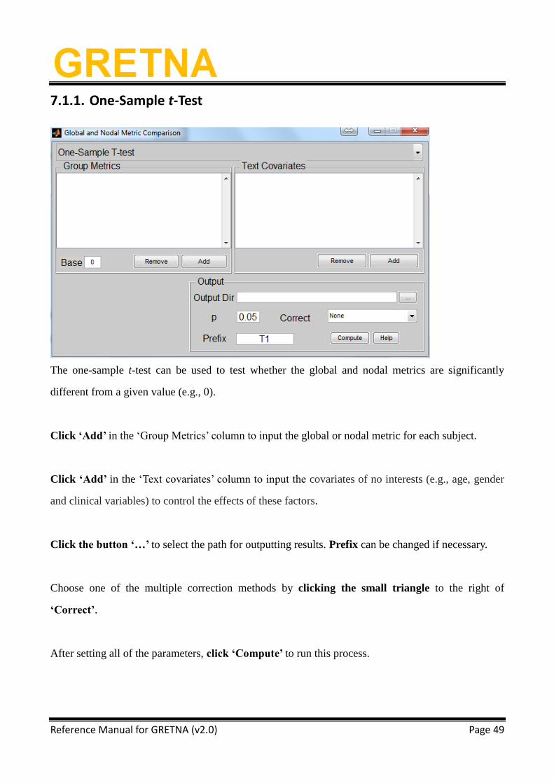
7.1.1. One-Sample t-Test
The one-sample t-test can be used to test whether the global and nodal metrics are significantly
different from a given value (e.g., 0).
Click ‘Add’ in the ‘Group Metrics’ column to input the global or nodal metric for each subject.
Click ‘Add’ in the ‘Text covariates’ column to input the covariates of no interests (e.g., age, gender
and clinical variables) to control the effects of these factors.
Click the button ‘…’ to select the path for outputting results. Prefix can be changed if necessary.
Choose one of the multiple correction methods by clicking the small triangle to the right of
‘Correct’.
After setting all of the parameters, click ‘Compute’ to run this process.
Page 50
Reference Manual for GRETNA (v2.0) Page 50
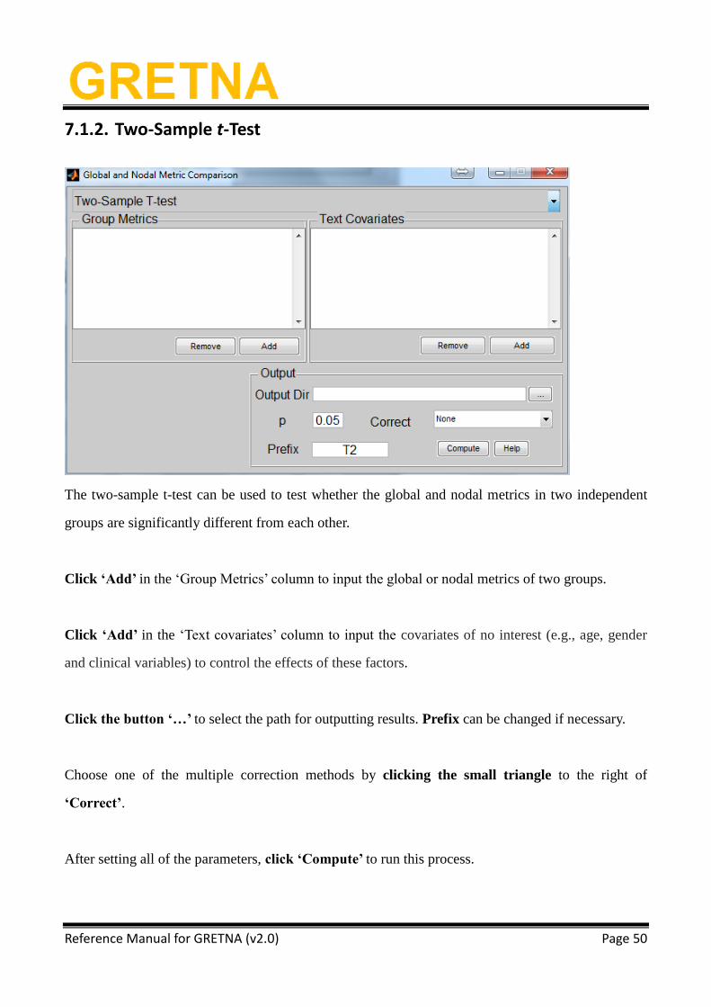
7.1.2. Two-Sample t-Test
The two-sample t-test can be used to test whether the global and nodal metrics in two independent
groups are significantly different from each other.
Click ‘Add’ in the ‘Group Metrics’ column to input the global or nodal metrics of two groups.
Click ‘Add’ in the ‘Text covariates’ column to input the covariates of no interest (e.g., age, gender
and clinical variables) to control the effects of these factors.
Click the button ‘…’ to select the path for outputting results. Prefix can be changed if necessary.
Choose one of the multiple correction methods by clicking the small triangle to the right of
‘Correct’.
After setting all of the parameters, click ‘Compute’ to run this process.
Page 51
Reference Manual for GRETNA (v2.0) Page 51
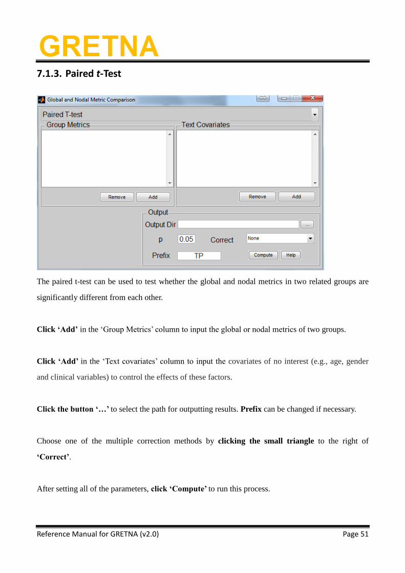
7.1.3. Paired t-Test
The paired t-test can be used to test whether the global and nodal metrics in two related groups are
significantly different from each other.
Click ‘Add’ in the ‘Group Metrics’ column to input the global or nodal metrics of two groups.
Click ‘Add’ in the ‘Text covariates’ column to input the covariates of no interest (e.g., age, gender
and clinical variables) to control the effects of these factors.
Click the button ‘…’ to select the path for outputting results. Prefix can be changed if necessary.
Choose one of the multiple correction methods by clicking the small triangle to the right of
‘Correct’.
After setting all of the parameters, click ‘Compute’ to run this process.
Page 52
Reference Manual for GRETNA (v2.0) Page 52
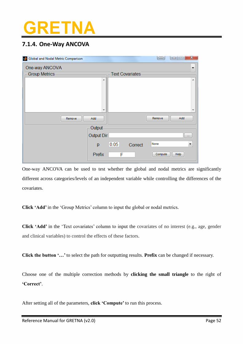
7.1.4. One-Way ANCOVA
One-way ANCOVA can be used to test whether the global and nodal metrics are significantly
different across categories/levels of an independent variable while controlling the differences of the
covariates.
Click ‘Add’ in the ‘Group Metrics’ column to input the global or nodal metrics.
Click ‘Add’ in the ‘Text covariates’ column to input the covariates of no interest (e.g., age, gender
and clinical variables) to control the effects of these factors.
Click the button ‘…’ to select the path for outputting results. Prefix can be changed if necessary.
Choose one of the multiple correction methods by clicking the small triangle to the right of
‘Correct’.
After setting all of the parameters, click ‘Compute’ to run this process.
Page 53
Reference Manual for GRETNA (v2.0) Page 53
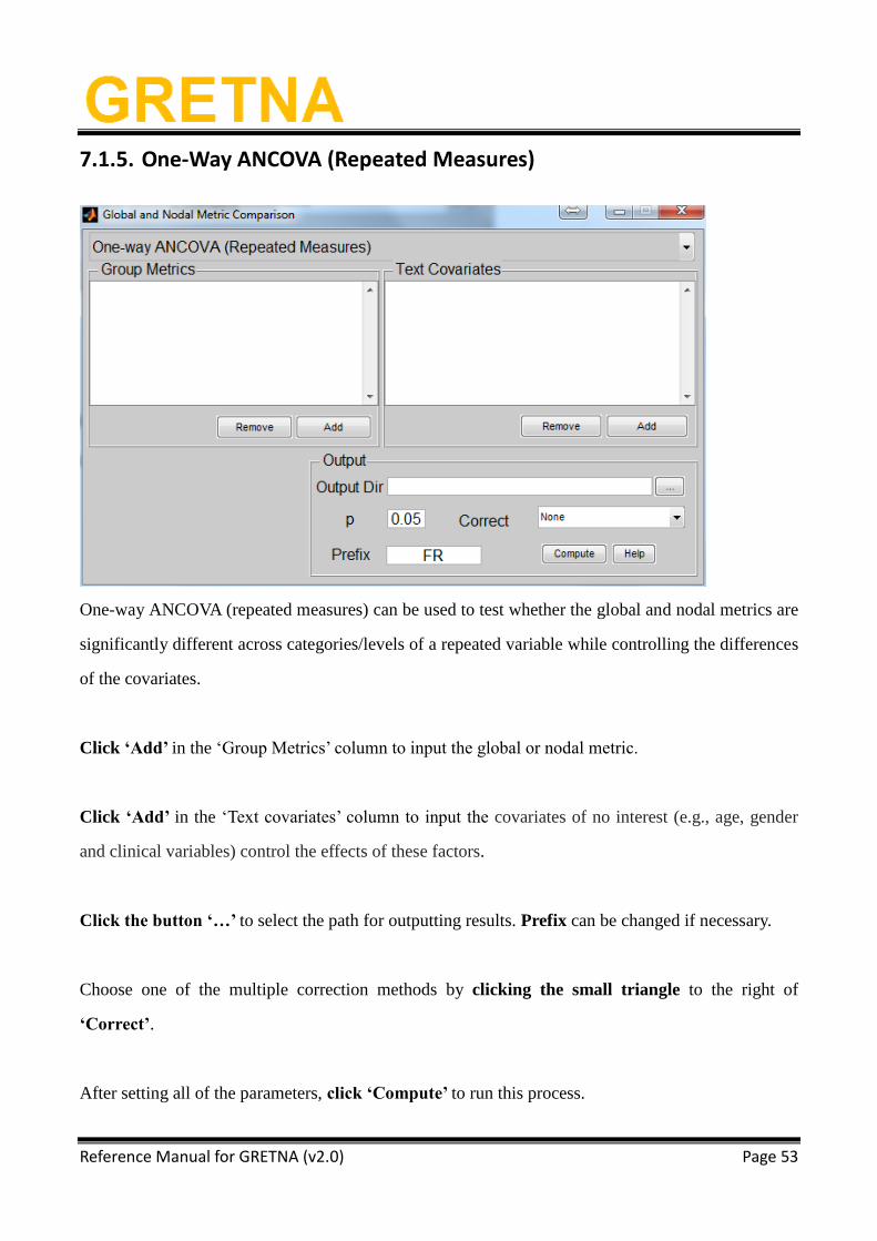
7.1.5. One-Way ANCOVA (Repeated Measures)
One-way ANCOVA (repeated measures) can be used to test whether the global and nodal metrics are
significantly different across categories/levels of a repeated variable while controlling the differences
of the covariates.
Click ‘Add’ in the ‘Group Metrics’ column to input the global or nodal metric.
Click ‘Add’ in the ‘Text covariates’ column to input the covariates of no interest (e.g., age, gender
and clinical variables) control the effects of these factors.
Click the button ‘…’ to select the path for outputting results. Prefix can be changed if necessary.
Choose one of the multiple correction methods by clicking the small triangle to the right of
‘Correct’.
After setting all of the parameters, click ‘Compute’ to run this process.
Page 54
Reference Manual for GRETNA (v2.0) Page 54
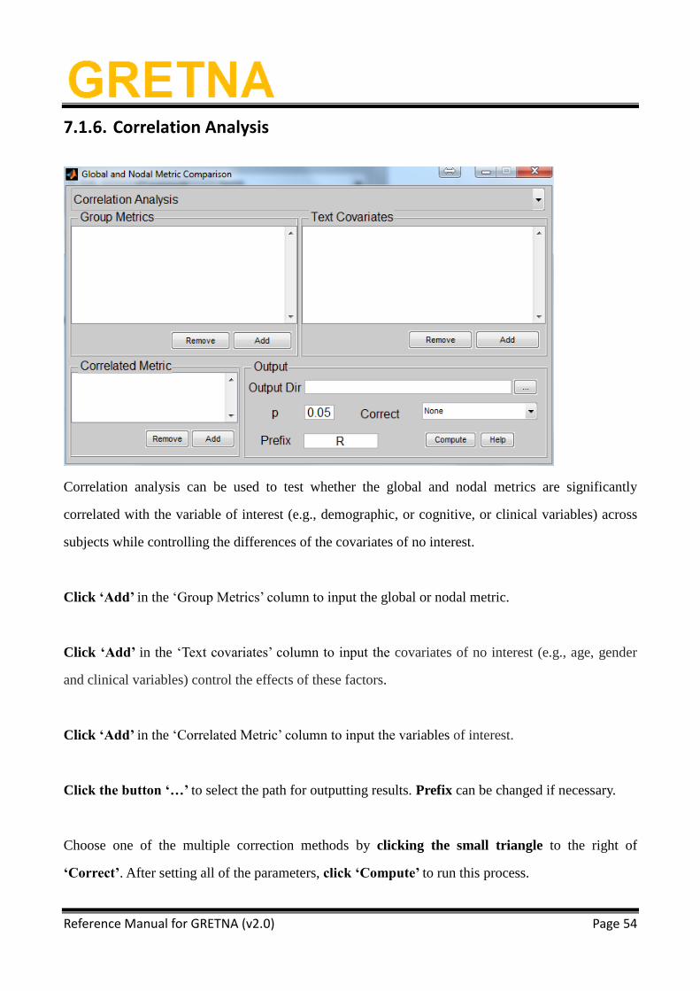
7.1.6. Correlation Analysis
Correlation analysis can be used to test whether the global and nodal metrics are significantly
correlated with the variable of interest (e.g., demographic, or cognitive, or clinical variables) across
subjects while controlling the differences of the covariates of no interest.
Click ‘Add’ in the ‘Group Metrics’ column to input the global or nodal metric.
Click ‘Add’ in the ‘Text covariates’ column to input the covariates of no interest (e.g., age, gender
and clinical variables) control the effects of these factors.
Click ‘Add’ in the ‘Correlated Metric’ column to input the variables of interest.
Click the button ‘…’ to select the path for outputting results. Prefix can be changed if necessary.
Choose one of the multiple correction methods by clicking the small triangle to the right of
‘Correct’. After setting all of the parameters, click ‘Compute’ to run this process.
Page 55
Reference Manual for GRETNA (v2.0) Page 55
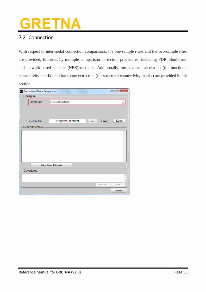
7.2. Connection
With respect to inter-nodal connection comparisons, the one-sample t-test and the two-sample t-test
are provided, followed by multiple comparison correction procedures, including FDR, Bonferroni
and network-based statistic (NBS) methods. Additionally, mean value calculation (for functional
connectivity matrix) and backbone extraction (for structural connectivity matrix) are provided in this
section.
Page 56
Reference Manual for GRETNA (v2.0) Page 56
7.2.1. Averaged (Functional)
Averaged (Functional) can be used to calculate the mean functional connectivity across subjects.
Click ‘Select Group 1 Network’ in the ‘Network Matrix’ column to input the matrix for each
subject in a group.
Click the button ‘…’ to select the path for outputting results. Prefix can be changed if necessary.
Click ‘Compute’ to run.
Page 57
Reference Manual for GRETNA (v2.0) Page 57
7.2.2. Backbone (Structural)
Backbone (Structural) can be used to extract the backbone of structural connectivity across
subjects.
Click ‘Select Group 1 Network’ in the ‘Network Matrix’ column to input the matrix for each
subject in a group.
Threshold Type refers to edge probability more options will be added in a future release).
Threshold Value can be changed according to your research purposes.
Click the button ‘…’ to select the path for outputting results. Prefix can be changed if necessary.
Click ‘Compute’ to run.
Page 58
Reference Manual for GRETNA (v2.0) Page 58
7.2.3. One-Sample t-Test
One-Sample T-test can be used to examine whether each connection significantly differs from a
given value (e.g., 0).
Click ‘Select Group 1 Network’ in the ‘Network Matrix’ column to input the matrix for each
subject in a group. You can then click ‘Add’ in the ‘covariates’ column to input the covariates of no
interest.
You can choose one of the following Correct Methods: FDR, Bonferroni, NBS, or None. You can
input a network mask to restrict the statistical scope and set the p value of the NBS component and
the number of iterations if you choose NBS.
Click the button ‘…’ to select the path for outputting results. Prefix can be changed if necessary.
Click ‘Compute’ to run.
Page 59
Reference Manual for GRETNA (v2.0) Page 59
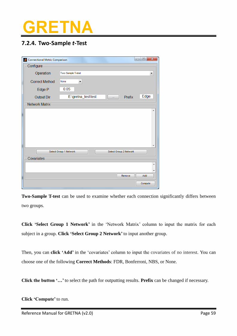
7.2.4. Two-Sample t-Test
Two-Sample T-test can be used to examine whether each connection significantly differs between
two groups.
Click ‘Select Group 1 Network’ in the ‘Network Matrix’ column to input the matrix for each
subject in a group. Click ‘Select Group 2 Network’ to input another group.
Then, you can click ‘Add’ in the ‘covariates’ column to input the covariates of no interest. You can
choose one of the following Correct Methods: FDR, Bonferroni, NBS, or None.
Click the button ‘…’ to select the path for outputting results. Prefix can be changed if necessary.
Click ‘Compute’ to run.
Page 60
Reference Manual for GRETNA (v2.0) Page 60
7.3. Results of Metric Comparison
7.3.1. Network and Node
One-Sample T-test
T1_PVector: The p value derived from a one-sample t-test on network metrics for each threshold.
T1_PThrd: The significance threshold of p values after correction of multiple comparisons.
T1_TVector: The t value derived from a one-sample t-test on network metrics for each threshold.
T1_TThrd: The significance threshold of t values after correction of multiple comparisons.
Two-Sample T-test
T2_PVector: The p value derived from a two-sample t-test on network metrics for each threshold.
T2_PThrd: The significance threshold of p values after correction of multiple comparisons.
T2_TVector: The t value derived from a two-sample t-test on network metrics for each threshold.
T2_TThrd: The significance threshold of t values after correction of multiple comparisons.
Paired T-test
TP_PVector: The p value derived from a paired t-test on network metrics for each threshold.
TP_PThrd: The significance threshold of p values after correction of multiple comparisons.
TP_TVector: The t value derived from a paired t-test on network metrics for each threshold.
Page 61
Reference Manual for GRETNA (v2.0) Page 61
TP_TThrd: The significance threshold of t values after correction of multiple comparisons.
One-way ANCOVA
F_FVector: The F value derived from one-way ANCOVA on network metrics for each threshold.
F_FThrd: The significance threshold of F values after correction of multiple comparisons.
F_PVector: The p value derived from one-way ANCOVA on network metrics for each threshold.
F_PThrd: The significance threshold of p values after correction of multiple comparisons.
One-way ANCOVA (Repeated Measures)
FR_FVector: The F value derived from repeated one-way ANCOVA on network metrics for each
threshold.
FR_FThrd: The significance threshold of F values after correction of multiple comparisons.
FR_PVector: The p value derived from repeated one-way ANCOVA on network metrics for each
threshold.
FR_PThrd: The significance threshold of p values after correction of multiple comparisons.
Correlation Analysis
R_PVector: The p value derived from correlation analysis between two metrics.
R_PThrd: The significance threshold of p values after correction of multiple comparisons.
R_RVector: The r value derived from correlation analysis between two metrics.
R_RThrd: The significance threshold of r values after correction of multiple comparisons.
Page 62
Reference Manual for GRETNA (v2.0) Page 62
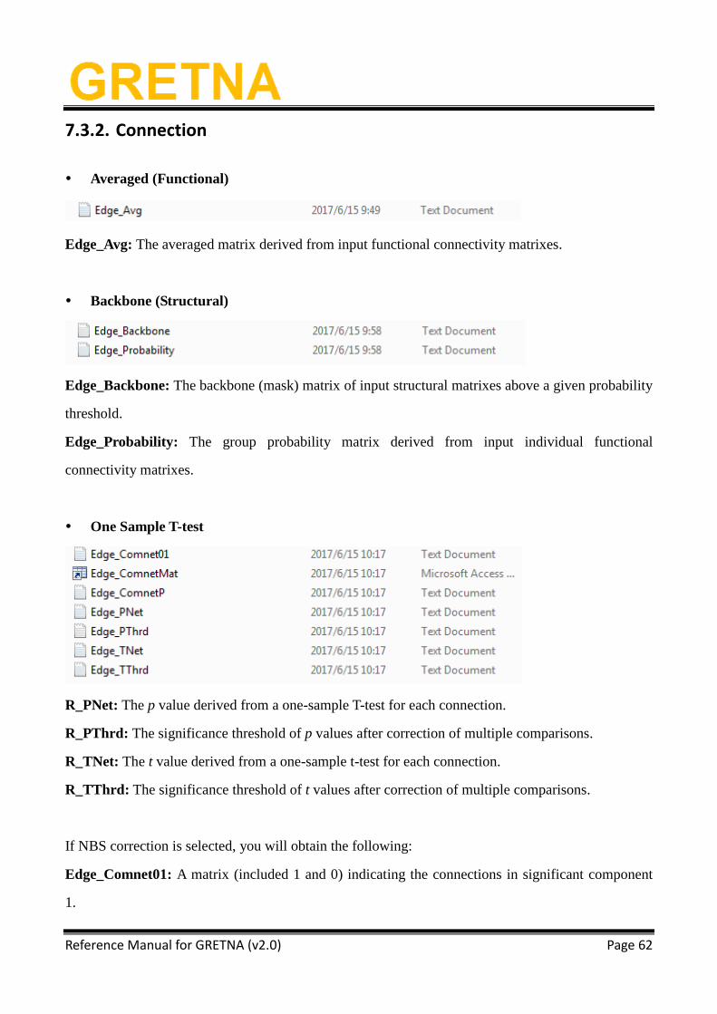
7.3.2. Connection
Averaged (Functional)
Edge_Avg: The averaged matrix derived from input functional connectivity matrixes.
Backbone (Structural)
Edge_Backbone: The backbone (mask) matrix of input structural matrixes above a given probability
threshold.
Edge_Probability: The group probability matrix derived from input individual functional
connectivity matrixes.
One Sample T-test
R_PNet: The p value derived from a one-sample T-test for each connection.
R_PThrd: The significance threshold of p values after correction of multiple comparisons.
R_TNet: The t value derived from a one-sample t-test for each connection.
R_TThrd: The significance threshold of t values after correction of multiple comparisons.
If NBS correction is selected, you will obtain the following:
Edge_Comnet01: A matrix (included 1 and 0) indicating the connections in significant component
1.
Page 63
Reference Manual for GRETNA (v2.0) Page 63
Edge_ComnetP: The p value derived from NBS for each component.
Edge_ComnetMat: A MAT-file including p value of the component and matrix mask for significant
components.
These files cannot be obtained if no significant results after NBS correction.
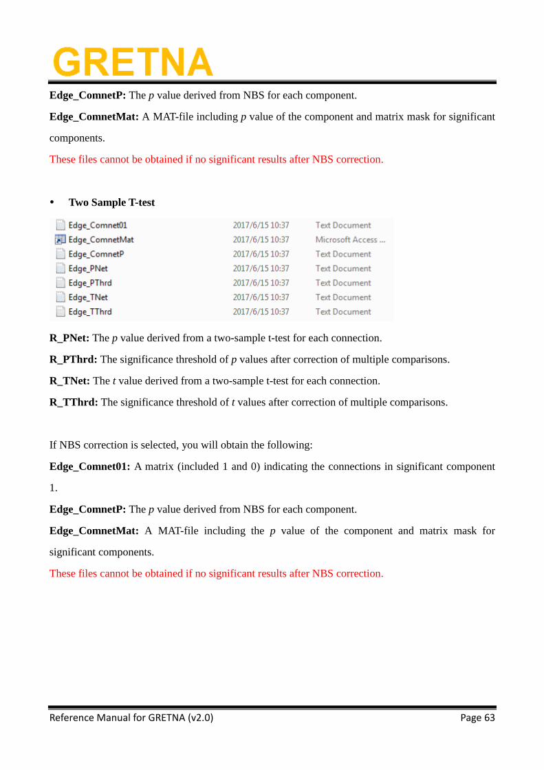
Two Sample T-test
R_PNet: The p value derived from a two-sample t-test for each connection.
R_PThrd: The significance threshold of p values after correction of multiple comparisons.
R_TNet: The t value derived from a two-sample t-test for each connection.
R_TThrd: The significance threshold of t values after correction of multiple comparisons.
If NBS correction is selected, you will obtain the following:
Edge_Comnet01: A matrix (included 1 and 0) indicating the connections in significant component
1.
Edge_ComnetP: The p value derived from NBS for each component.
Edge_ComnetMat: A MAT-file including the p value of the component and matrix mask for
significant components.
These files cannot be obtained if no significant results after NBS correction.
Page 64
Reference Manual for GRETNA (v2.0) Page 64
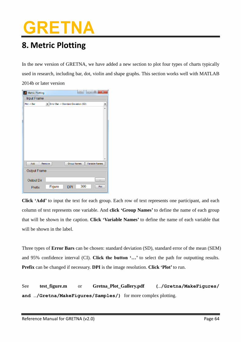
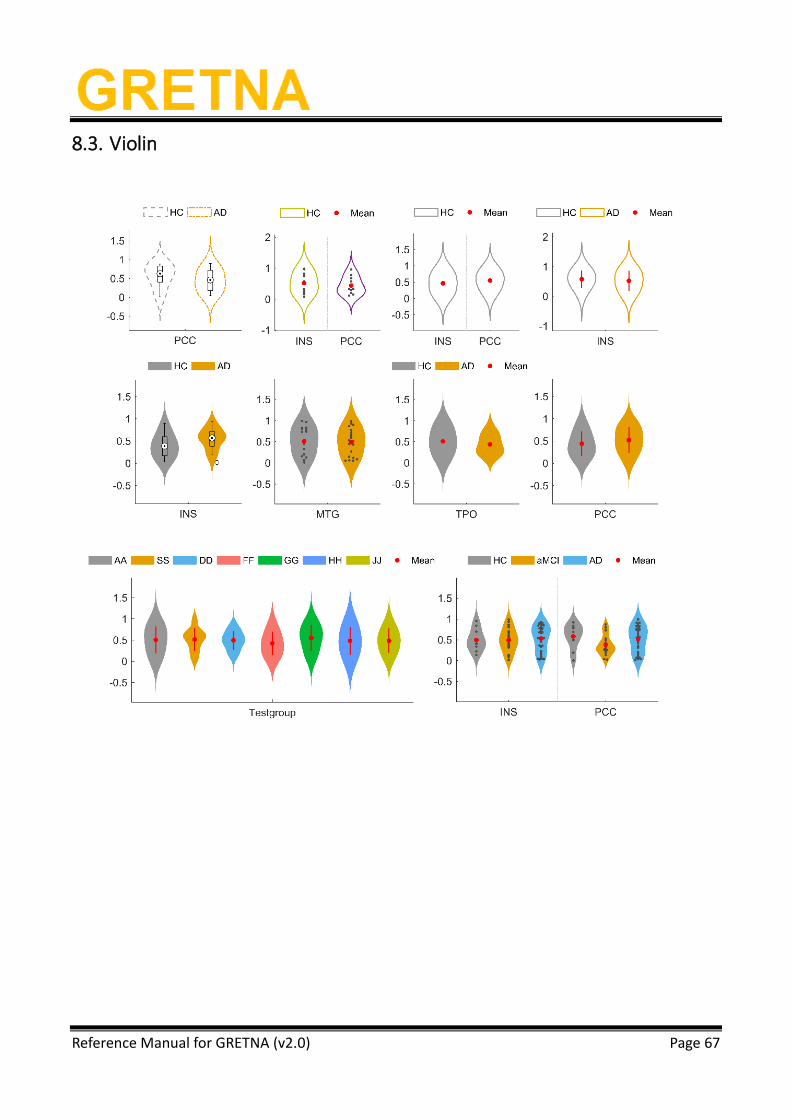
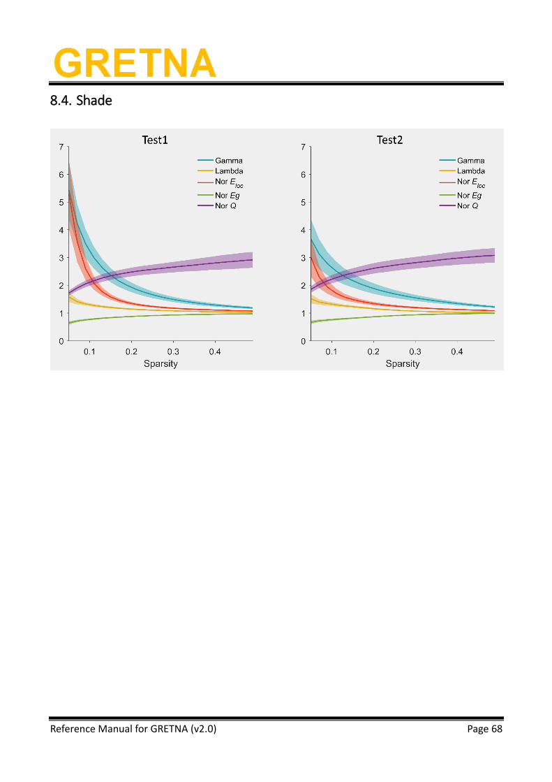
8. Metric Plotting
In the new version of GRETNA, we have added a new section to plot four types of charts typically
used in research, including bar, dot, violin and shape graphs. This section works well with MATLAB
2014b or later version
Click ‘Add’ to input the text for each group. Each row of text represents one participant, and each
column of text represents one variable. And click ‘Group Names’ to define the name of each group
that will be shown in the caption. Click ‘Variable Names’ to define the name of each variable that
will be shown in the label.
Three types of Error Bars can be chosen: standard deviation (SD), standard error of the mean (SEM)
and 95% confidence interval (CI). Click the button ‘…’ to select the path for outputting results.
Prefix can be changed if necessary. DPI is the image resolution. Click ‘Plot’ to run.
See test_figure.m or Gretna_Plot_Gallery.pdf (…/Gretna/MakeFigures/
and …/Gretna/MakeFigures/Samples/) for more complex plotting.
Page 65
Reference Manual for GRETNA (v2.0) Page 65
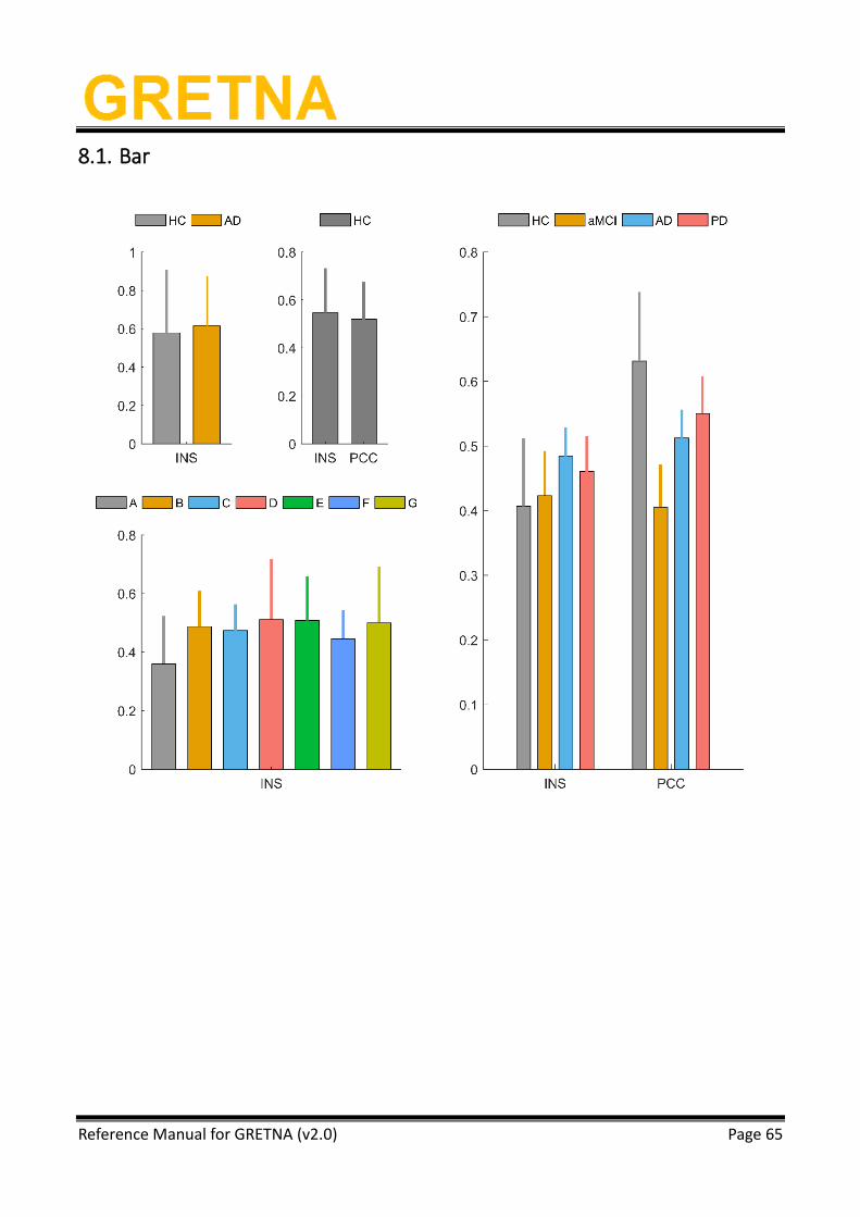
8.1. Bar
Page 66
Reference Manual for GRETNA (v2.0) Page 66
8.2. Dot
Page 67
Reference Manual for GRETNA (v2.0) Page 67
8.3. Violin
Page 68
Reference Manual for GRETNA (v2.0) Page 68
8.4. Shade
Page 69
Reference Manual for GRETNA (v2.0) Page 69
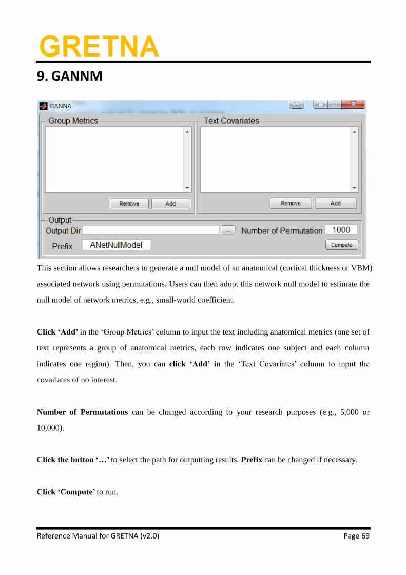
9. GANNM
This section allows researchers to generate a null model of an anatomical (cortical thickness or VBM)
associated network using permutations. Users can then adopt this network null model to estimate the
null model of network metrics, e.g., small-world coefficient.
Click ‘Add’ in the ‘Group Metrics’ column to input the text including anatomical metrics (one set of
text represents a group of anatomical metrics, each row indicates one subject and each column
indicates one region). Then, you can click ‘Add’ in the ‘Text Covariates’ column to input the
covariates of no interest.
Number of Permutations can be changed according to your research purposes (e.g., 5,000 or
10,000).
Click the button ‘…’ to select the path for outputting results. Prefix can be changed if necessary.
Click ‘Compute’ to run.
Page 70
Reference Manual for GRETNA (v2.0) Page 70
Acknowledgements
We thank the following colleagues for their kind helps during GRETNA developing and testing:
Mingrui Xia, Xuhong Liao, Miao Cao, Zhengjia Dai, Hao Wang, Zhijiang Wang, Jin Liu, Xiaodan
Chen, Yuehua Xu, Zhilei Xu, Qing Ma, Yapei Xie, Xiaoyi Sun, Siqi Wang, Rui Hou, Junjiao Feng,
Feng Liu (Tianjin Medical University General Hospital), Qiang Xu (Tianjin Medical University
General Hospital), Tao Liu (Beihang University), Chao Dong (Beihang University), Lei Gao
(Zhongnan Hospital),Wei Cheng (Fudan University) and Professor Alan Evans (McGill University,
Canada)
We thank the following colleagues for their efforts in manual revising:
Jin Liu, Miao Cao, Xindi Wang
We also thank the developers of the following softwares and toolboxes whose source codes or file
formats were referenced during our package developing:
Matlab: www.mathworks.com/products/matlab/
MatlabBGL: www.cs.purdue.edu/homes/dgleich/packages/matlab_bgl/
MRIcroN: www.mccauslandcenter.sc.edu/mricro/mricron/
Brain Connectivity Toolbox: sites.google.com/site/bctnet/
SPM: www.fil.ion.ucl.ac.uk/spm/
REST: www.restfmri.net/
Page 71
Reference Manual for GRETNA (v2.0) Page 71
Reference
Cui Z, Zhong S, Xu P, He Y, Gong G (2013): PANDA: a pipeline toolbox for analyzing brain
diffusion images. Front Hum Neurosci 7:42.
Maslov S, Sneppen K (2002): Specificity and stability in topology of protein networks. Science
296:910-913.
Ravasz E, Barabási A-L (2003): Hierarchical organization in complex networks. Phys. Rev. E.
67:026112.
Rubinov M, Sporns O (2010): Complex network measures of brain connectivity: uses and
interpretations. Neuroimage 52:1059-69.
Wang JH, Zuo XN, Gohel S, Milham MP, Biswal BB, He Y (2011): Graph theoretical analysis of
functional brain networks: test-retest evaluation on short- and long-term resting-state
functional MRI data. PLoS One 6:e21976.


![PnPMPCToolboxv. 1.0-Usermanual1 - sisdin.unipv.itsisdin.unipv.it/pnpmpc/phpinclude/toolbox/PnPMPC-toolbox...• GraphViz4MatLab toolbox [9] that allows one to plot the graph of a large-scale](https://static.documents.pub/doc/80x56/608db6b6c8c78247ff231972/pnpmpctoolboxv-10-usermanual1-a-graphviz4matlab-toolbox-9-that-allows.jpg)


