A Graphical Exposition of the GTAP Model by Martina BROCKMEIER GTAP Technical Paper No. 8 October 1996 Minor Edits, January 2000 Revised, March 2001 BROCKMEIER is with the Institute of Agricultural Economics, Justus Liebig University Giessen, Giessen, Germany. GTAP stands for the Global Trade Analysis Project which is administered by the Center for Global Trade Analysis, Purdue University, West Lafayette, IN 47907-1145 USA. For more information about GTAP, please refer to our Worldwide Web site at http://www.agecon.purdue.edu/gtap/, or send a request to [email protected].
Transcript
A Graphical Exposition of the GTAP Model
by Martina BROCKMEIER
GTAP Technical Paper No. 8
October 1996Minor Edits, January 2000
Revised, March 2001
BROCKMEIER is with the Institute of Agricultural Economics, Justus Liebig University Giessen, Giessen,
Germany.
GTAP stands for the Global Trade Analysis Project which is administered by the Center for Global Trade
Analysis, Purdue University, West Lafayette, IN 47907-1145 USA. For more information about GTAP, please
refer to our Worldwide Web site at http://www.agecon.purdue.edu/gtap/, or send a request to
This paper offers a graphical exposition of the GTAP model of global trade. Particular emphasis isplaced on the accounting, or equilibrium, relationships in the model. It begins with a treatment ofthe a one region version of GTAP, thereafter adding a rest of world region to highlight the treatmentof trade flows in the model. The implementation of policy instruments in GTAP is also explored,using simple supply-demand graphics. The material provided in this paper was first developed as anintroduction to GTAP for participants taking the annual short course. Based on its success in thatvenue, this paper has been placed on the “highly recommended” reading list for individuals seekingan introduction and overview of the GTAP framework. It was modified in March of 2001 to reflectthe changes in version 6.0 of the GTAP model.
Figure 7: Export Subsidy or Tax in Region r on Sales to Region s . . . . . . . . . . . . . . . . . 18
Figure 8: Import Subsidy or Tax in Region s on Purchases from Region r . . . . . . . . . . . 19
4
A Graphical Exposition of theGTAP Model
1. IntroductionOver the last several decades Applied General Equilibrium (AGE) models has become an important
tool for analyzing economic issues. This development is explained by the capability of AGE models
to provide an elaborate and realistic representation of the economy including the linkages between
all agents, sectors and other economies. While this complete coverage permits a unique insight into
the effects of changes in the economic environment throughout the whole economy, single country,
and especially global AGE models very often include an enormous number of variables, parameters
and equations.
GTAP (Global Trade Analysis Project) is a multi-regional AGE model which captures world
economic activity in 57 different industries of 66 regions (Version 5 of the data base). However, the
theory behind the GTAP model is similar to that of other standard, multi- regional AGE models. The
underlying equation system of GTAP accordingly includes two different kinds of equations. One part
covers the accounting relationships which ensure that receipts and expenditures of every agent in
the economy are balanced. The other part of the equation system consists of behavioral equations
which based upon microeconomic theory. These equations specify the behavior of optimizing agents
in the economy, such as demand functions.
Given the large number of components necessary to build GTAP, it is not easy to get a general idea
of the theory behind the model. For this reason, the following documentation gives an overview of
the model structure by focusing on the accounting relationships. It provides a useful companion to
chapter 2 of the GTAP book (HERTEL, 1997) in which the theory behind the model and especially
the derivation of the behavioral equations are covered in more detail.
This paper is organized as follows. The first section presents the accounting relationships in a closed
economy version of the GTAP model without government intervention. There, the generation and
distribution of income as well as domestic demand and supply are discussed. In the following
section, taxes and subsidies are introduced into this closed economy. The implementation of policy
instruments changes most parts of the model structure. Therefore, the accounting relationships in
the one region model are considered once again. Additionally, the computation of tax revenues and
subsidy expenditures are discussed in detail. In the third section, the closed economy is then
extended to a multi-region version of GTAP which includes a trading sector. Finally, an assessment
of the accounting relationships in an open economy and the computation of subsidies and taxes
implemented in the trading sector completes this graphical exposition of the GTAP model.
1.The reason expenditure shares are not constant, as might be expected in a Cobb-Douglas demand system, is that the
private expenditure function is non-homothetic and therefore the “price” of private consumption depends on the amount
“purchased.” Accommodating this endogeneity in the regional households’ optimization problem results in a new set of
demand equations in which the shares are non-constant. See McDougall, 2001, for a complete exposition of the new final
demand system in the version 6.0 GTAP model.
2. The new theory of regional household demand developed by McDougall (2001) permits the user to fix any one of these
components of final demand by shifting preferences. Thus, for example, the level of government activities could be fixed,
and the associated preference parameter permitted to vary. In this way the regional household is assured of remaining on
its budget constraint, and welfare analysis may still be conducted – albeit with allowance for the impact of changing
preferences. See McDougall (2001) for details.
3. Every value flow which is initiated by introducing a new agent into the graph is in bold. This procedure is also given
in each of the following graphs.
4. In this specification VOA is the value added actually received by the private household in return for the use of its
endowments. Endowment commodities are non-tradeable goods which include agricultural land, labor and capital.
5
2. One Region Closed Economy WithoutGovernment Interventions
The following graphical illustration will explain the basic concept of GTAP by focusing on the
accounting relationships. Different economic activities are introduced step by step into these figures.
In so doing, one agent after the other is added to the graph, and thereby the GTAP model is
developed piece by piece.
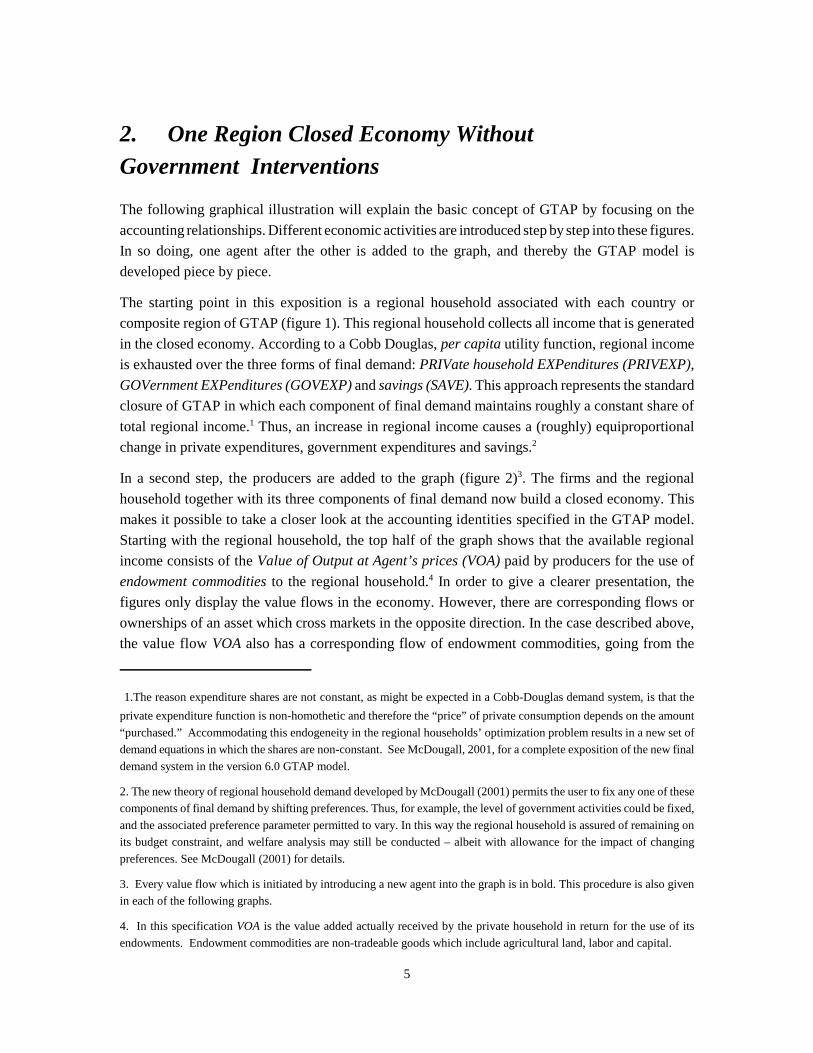
The starting point in this exposition is a regional household associated with each country or
composite region of GTAP (figure 1). This regional household collects all income that is generated
in the closed economy. According to a Cobb Douglas, per capita utility function, regional income
is exhausted over the three forms of final demand: PRIVate household EXPenditures (PRIVEXP),
GOVernment EXPenditures (GOVEXP) and savings (SAVE). This approach represents the standard
closure of GTAP in which each component of final demand maintains roughly a constant share of
total regional income.1 Thus, an increase in regional income causes a (roughly) equiproportional
change in private expenditures, government expenditures and savings.2
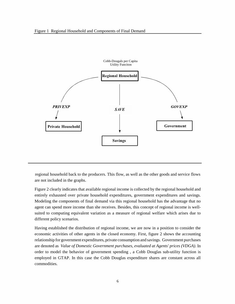
In a second step, the producers are added to the graph (figure 2)3. The firms and the regional
household together with its three components of final demand now build a closed economy. This
makes it possible to take a closer look at the accounting identities specified in the GTAP model.
Starting with the regional household, the top half of the graph shows that the available regional
income consists of the Value of Output at Agent’s prices (VOA) paid by producers for the use of
endowment commodities to the regional household.4 In order to give a clearer presentation, the
figures only display the value flows in the economy. However, there are corresponding flows or
ownerships of an asset which cross markets in the opposite direction. In the case described above,
the value flow VOA also has a corresponding flow of endowment commodities, going from the
6
Figure 1 Regional Household and Components of Final Demand
regional household back to the producers. This flow, as well as the other goods and service flows
are not included in the graphs.
Figure 2 clearly indicates that available regional income is collected by the regional household and
entirely exhausted over private household expenditures, government expenditures and savings.
Modeling the components of final demand via this regional household has the advantage that no
agent can spend more income than she receives. Besides, this concept of regional income is well-
suited to computing equivalent variation as a measure of regional welfare which arises due to
different policy scenarios.
Having established the distribution of regional income, we are now in a position to consider the
economic activities of other agents in the closed economy. First, figure 2 shows the accounting
relationship for government expenditures, private consumption and savings. Government purchases
are denoted as Value of Domestic Government purchases, evaluated at Agents' prices (VDGA). In
order to model the behavior of government spending , a Cobb Douglas sub-utility function is
employed in GTAP. In this case the Cobb Douglas expenditure shares are constant across all
commodities.
Cobb-Dougals per Capita Utility Funciton
7
Figure 2 One Region Closed Economy without Government Intervention
5. Since firms gets revenue for selling their goods to other producers on the one hand and buy intermediate inputs onthe other hand, these values flow in both direction.
8
The second component of final demand is private consumption (Value of Domestic Private
household purchases, evaluated at Agents' prices, VDPA). The constrained optimizing behavior of
private consumption is represented in GTAP by the CDE (Constant Difference of Elasticity)
implicit expenditure function. The CDE function is less general than the fully flexible functional
forms on the one hand, but more flexible than the commonly used CES/LES functions on the other
hand. It is easily calibrated using data on income and own price elasticities of demand (for more
detail see HERTEL, et.al., 1991).
Considering the third component of final demand, figure 2 shows that savings are completely
exhausted on investment (NETINV). In GTAP the demand for investment is savings-driven. Given
the static nature of the GTAP model, current investment is assumed not to be installed during the
considered period, and therefore does not affect the productive capability of the industries in the
model. However, the demand for investment goods will affect the economic activity in the region
through its effects on the pattern of production. The mix of capital goods used for investment is
treated in a manner analogous to the modeling of intermediate demand which is discussed below.
Looking at the production side of the closed economy, figure 2 also shows the accounting
relationships of firms in GTAP. The producers receive payments for selling consumption goods to
the private households (VDPA) and the government (VDGA), intermediate inputs to other producers
(Value of Domestic Firm Purchases, evaluated at Agents’ prices, VDFA) and investment goods to
the savings sector (NETINV). Under the zero profit assumption employed in GTAP, these revenues
must be precisely exhausted on expenditures for intermediate inputs (VDFA) and primary factors of
production (VOA).5
The nested production technology in GTAP exhibits constant returns to scale and every sector
produces a single output. Furthermore, it is assumed the technology is weakly separable between
primary factors of production and intermediate inputs. Profit maximizing firms therefore choose their
optimal mix of primary factors independently of the prices of intermediate inputs. Utilizing this type
of separability also means that the elasticity of substitution between any individual primary factor
and different intermediate inputs is equal. This technology is further simplified by employing the
Constant Elasticity of Substitution (CES) functional form in the aggregation of primary factors, as
well as in the combination of value-added and intermediate inputs in order to produce output. This
reduces the total number of substitution parameters in the production function to two per sector.
Among the primary factors, the GTAP model additionally distinguishes between endowment
commodities which are perfectly mobile and those which are sluggish to adjust. In the former case,
the factor earns the same market return regardless of where it is employed. In the case of sluggish
endowment commodities, returns in equilibrium may differ across sectors.
The complete accounting relationships in this one region closed economy model form a simultaneous
equation system in which one identity is redundant and can be dropped. In GTAP the savings-
6. In the original GTAP model, the price of savings was chosen as the numeraire. In the version 6.0 model the price ofsavings varies by region. Here the global average return to primary factors is typically used as the numeraire.
7. If subsidies to the private households (firms) are higher than taxes, the value flow presents additional income(revenue).
9
investment identity is not imposed. A separate computation of savings and investment therefore
offers a consistency check on the accounting relationships and verifies that Walras' Law is satisfied.
Since the model can only be solved for N-1 prices, the one price is set exogenously, and all other
prices are evaluated relative to this numeraire.6
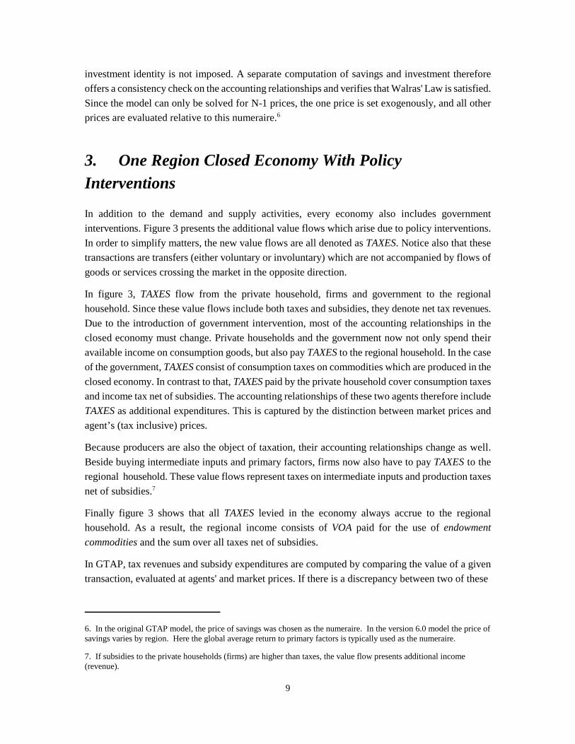
3. One Region Closed Economy With PolicyInterventions
In addition to the demand and supply activities, every economy also includes government
interventions. Figure 3 presents the additional value flows which arise due to policy interventions.
In order to simplify matters, the new value flows are all denoted as TAXES. Notice also that these
transactions are transfers (either voluntary or involuntary) which are not accompanied by flows of
goods or services crossing the market in the opposite direction.
In figure 3, TAXES flow from the private household, firms and government to the regional
household. Since these value flows include both taxes and subsidies, they denote net tax revenues.
Due to the introduction of government intervention, most of the accounting relationships in the
closed economy must change. Private households and the government now not only spend their
available income on consumption goods, but also pay TAXES to the regional household. In the case
of the government, TAXES consist of consumption taxes on commodities which are produced in the
closed economy. In contrast to that, TAXES paid by the private household cover consumption taxes
and income tax net of subsidies. The accounting relationships of these two agents therefore include
TAXES as additional expenditures. This is captured by the distinction between market prices and
agent’s (tax inclusive) prices.
Because producers are also the object of taxation, their accounting relationships change as well.
Beside buying intermediate inputs and primary factors, firms now also have to pay TAXES to the
regional household. These value flows represent taxes on intermediate inputs and production taxes
net of subsidies.7
Finally figure 3 shows that all TAXES levied in the economy always accrue to the regional
household. As a result, the regional income consists of VOA paid for the use of endowment
commodities and the sum over all taxes net of subsidies.
In GTAP, tax revenues and subsidy expenditures are computed by comparing the value of a given
transaction, evaluated at agents' and market prices. If there is a discrepancy between two of these
10
Figure 3 One Region Closed Economy with Government Intervention
11
values, then the difference must be equal to the tax or subsidy in question. Thus, the approach used
here neither keeps track of any individual tax and subsidy, nor of the different possible uses of these
tax revenues (i.e. increased government purchases, reduced public sector deficit).Taxes and subsidies
drive a wedge between the market price and the agents' price. In GTAP this linkage is taken into
account by multiplying the market price of the particular commodity by the power of the associated
ad valorem tax or subsidy, whereby the agents' price of the commodity is obtained. According to the
demand and supply elasticities in the individual market, the market price as well as the agents' price
in the new equilibrium will be changed. Whether the resulting agents' price will be higher or lower
than the associated market price depends on which agent pays the tax. In the case of a tax (subsidy)
on the demand side, the agents' price is higher (lower) than the market price. If the tax (subsidy) is
imposed on supplier of the particular commodity, the agents' price is lower (higher) than the market
price.
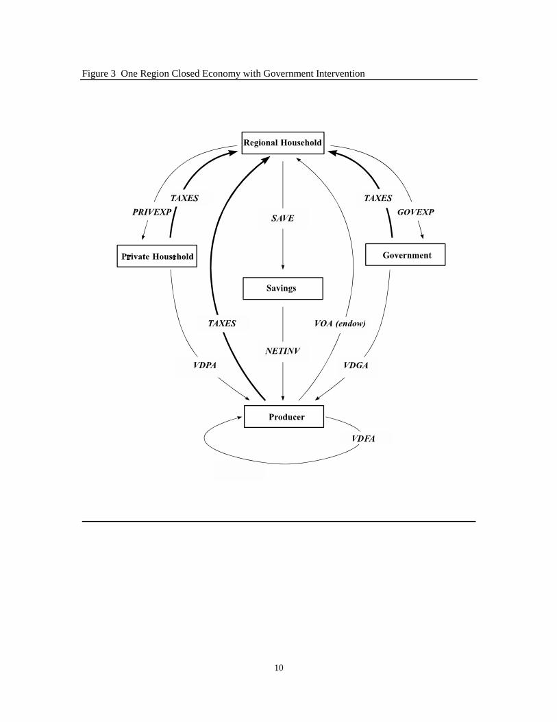
Figures 4 and 5 show these relations in more detail. Here it is assumed that every other tax or
subsidy is equal to zero, except the particular intervention which is considered in the different parts
of these figures. Turning attention first to the tax on private household’s purchases, figure 4.1 shows
that in the initial equilibrium, the power of the ad valorem tax (TPD) is equal to one and the market
price (PM0) therefore equals the agents' price (PPD0). After imposing a tax on the private
household’s purchases of commodity I, the market price (PM1) is reduced, whereas the agents' price
(PPD1) is increased.
The power of the ad valorem tax in this case is given by the ratio of the Value of Domestic Private
household’s purchases evaluated at Agents' price (VDPA) to the Value of Domestic Private
household’s purchases evaluated at Market price (VDPM):
TPD = VDPA/VDPM
Since TPD is greater than one, the agents' price must be higher than the market price according to
the price linkage relationship PM � TPD = PPD. In a second step the tax revenues (DTAX) can be
computed by: DPTAX = VDPA - VDPM. These taxes are paid by the private household or the
consumption side and are included in the TAXES flowing to the regional household or the income
side in figure 3. Furthermore, VDPM indicates the revenues which are received by the producers for
selling their commodities.
Figure 4.2 represents the adjustments which have taken place after a subsidy on the private
household’s purchases of commodity i is implemented. In this instance, VDPM is greater than VDPA,
so that the power of the ad valorem tax, TPM, is smaller than one and the agents' price (PPD1) is
lower than the market price(PM1). Accordingly, DPTAX is negative and withdrawn from the regional
income. Thus, the TAXES flowing from the private household to the regional household represent
net tax revenues.
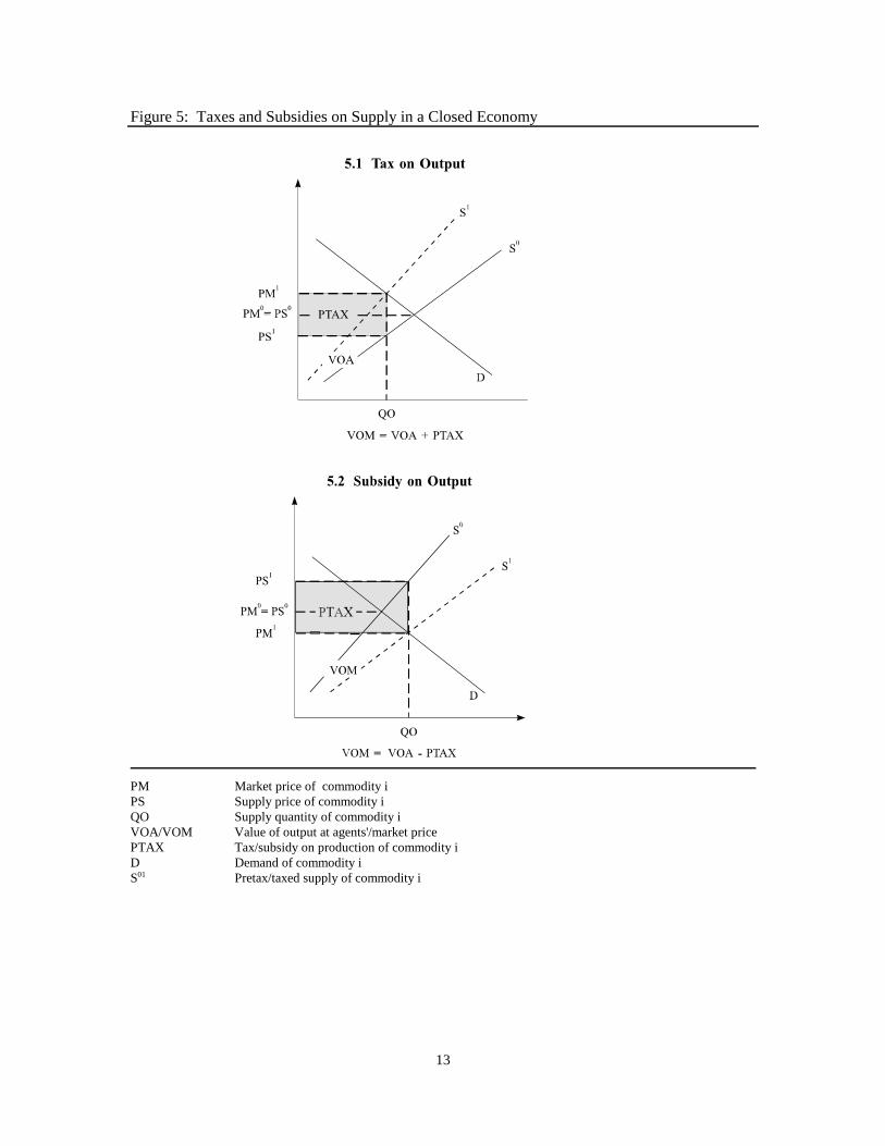
Figure 5 shows an intervention on the supply side. Here, a tax on output is considered first (figure
5.1). In the initial equilibrium, the power of the ad valorem tax, TO, equals one so that the agents'
price (PS0) and the market price (PM0) coincide. The introduction of a producer tax drives a wedge
12
DPTAX
DPTAX
Figure 4 Taxes and Subsidies on Demand in a Closed Economy
PM Market price of commodity iPPD Private household's price of commodity iQPD Private household demand for commodity iVDPA/VDPM Value of private household's purchases of commodity i valued at agents'/market priceDPTAX Tax/subsidy on commodity i purchased by private householdsD0,1 Pretax/taxed demand of commodity iS Supply of commodity i,
13
Figure 5: Taxes and Subsidies on Supply in a Closed Economy
PM Market price of commodity iPS Supply price of commodity iQO Supply quantity of commodity iVOA/VOM Value of output at agents'/market pricePTAX Tax/subsidy on production of commodity iD Demand of commodity iS01 Pretax/taxed supply of commodity i
8. GTAP actually includes a transportation sector which accounts for the difference between fob and cif values for aparticular commodity shipped along a particular route. This transportation sector is neglected in figure 6 in order toprovide a simpler presentation.
14
between these two prices. In contrast to taxation of the demand side, the agents' price (PS1) is now
lower than the market price (PM1). Therefore, the power of the ad valorem tax, calculated as the ratio
of the Value of Output at Agents' price (VOA) to the Value of Output evaluated at Market price
(VOM), is smaller than one. Producer tax revenue, PTAX, is given by the difference between VOM
and VOA:
PTAX = VOM - VOA
Because all taxes levied in the closed economy accrue to the regional household, these tax revenues
are included in the TAXES flowing from the producers to the regional household in figure 3.
Finally, figure 5.2 shows the price adjustments which occur after an implementation of a subsidy on
sales of commodity i. Here, the agents' price (PS1) lies above the market price (PM1).
Correspondingly, VOA is greater than VOM, and PTAX represents an expenditure which is
withdrawn from regional income.
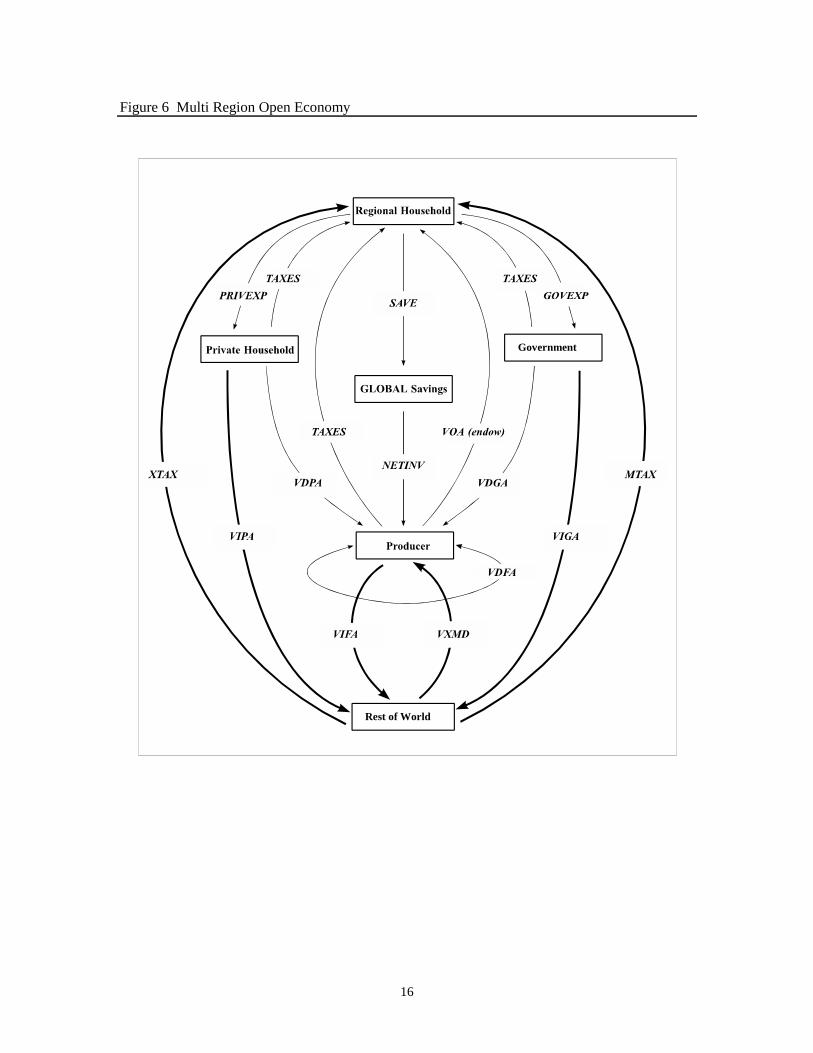
4. Multi-Region Open EconomyGiven knowledge of the theory behind the one region version of the GTAP model, we are now in a
position to integrate a trading sector into the model. How could this be done graphically? Actually,
there are two opportunities. One possibility would be to take all single countries and regions
included in GTAP, put them together in one graph and connect them to each other by drawing all
of the existing trade flows. Since the version 5.0 GTAP data base covers 66 regions, this would
certainly be too much for one graph! The other alternative is to combine all regions in the model
except one in a sector called Rest of the World. The one single region is then used to show the
changes in the model structure which has to be done in order to model an open economy. Since these
changes occur in every region of the multi region model, a complete overview is given by this
approach.
In figure 6, a sector called Rest of the World and the value flows initiated by this new agent are
added to the graph. Therefore, the graph represents a multi-region open economy in which the
accounting relationships of all agents have changed once again.8 Considering the production side of
the open economy, figure 6 indicates that firms on one side get additional revenues for selling
commodities to the Rest of the World. These exports are denoted by VXMD. On the other side, the
producers now spend their revenues not only on primary factors and domestically produced
intermediate inputs, but also on imported intermediate inputs, VIFA. Furthermore, the firms have to
pay an additional consumption tax on imported inputs to the regional household. Since this tax
15
expenditure is included in the TAXES flowing from the producer to regional household, the graph
does not show any change in this respect.
The GTAP model employs the so-called Armington assumption in the trading sector which provides
the possibility to distinguish imports by their origin and explains intra-industry trade of similar
products. Thus, imported commodities are assumed to be separable from domestically produced
goods and combined in an additional nest in the production tree. The elasticity of substitution in this
input nest is equal across all uses. Under these circumstances, the firms decide first on the sourcing
of their imports and based on the resulting composite import price, they then determine the optimal
mix of imported and domestic goods. In contrast to the closed economy, the multi- region model
therefore includes separate conditional demand equations for domestic and imported intermediate
inputs.
Figure 6 also shows the accounting relationships of the component of final demand in an open
economy. Here, the government and private households not only spend their income on domestically
produced but also on imported commodities which are denoted as VIPA and VIGA, respectively.
Furthermore, both agents have to pay additional commodity taxes on imports to the regional
household, so that the accounting relationships of these two agents now also include consumption
taxes and expenditure for imported commodities. Analogous to the firms behavior described above,
the multi region GTAP model includes conditional demand equations for imported commodities
reported for government and private consumption. Imported commodities and domestically
produced commodities are combined in a composite nest for both private and government
expenditures, respectively. The elasticity of substitution between imported and domestically
produced goods in this composite nest of the utility tree is assumed to be equal across uses. Firms
and households import demand equations therefore differ only in their import shares.
The accounting relationship of the third component of final demand, savings, has also changed.
Since these variations cannot easily be represented in the figure, the savings in figure 6 are denoted
simply as GLOBAL Savings. In the multi region version of the GTAP model, savings and investment
are computed on a global basis, so that all savers in the model face a common price for this savings
commodity. This means that if all other markets in the multi regional model are in equilibrium, all
firms earn zero profits, and all households are on their budget constraint, then global investment
must equal global savings and Walras' Law will be satisfied.
Finally, we have to check the accounting relationships for the rest of the world. According to the
graph, the rest of the world gets payments for selling their goods for private consumption,
government, and firms. These revenues will be spent on commodities exported from the single
region to the rest of the world, denoted as VXMD, and on import taxes, MTAX, and export taxes,
XTAX paid to the regional household.
Trade generated tax revenues and subsidy expenditures are computed in a manner analogous to the
ones which are being raised by policy instruments used in the domestic market. The only difference
is that now the tax or subsidy rates are defined as the ratio of market prices to world prices. If there
is an import tax (subsidy), the market price is higher (lower) than the world price, so that the power
16
Figure 6 Multi Region Open Economy
Government
Rest of World
9. Since the TAXES always represents net tax revenues, the tax flows from the regional household to all other agents in
the economy also include subsidy expenditures in the opposite direction which are not explicitly shown in figure 6.
17
of the ad valorem tax is greater (smaller) than one. In the case of an export tax (subsidy), the marketprice lies below (above) the world price and the power of the ad valorem tax is smaller (greater) thanone.
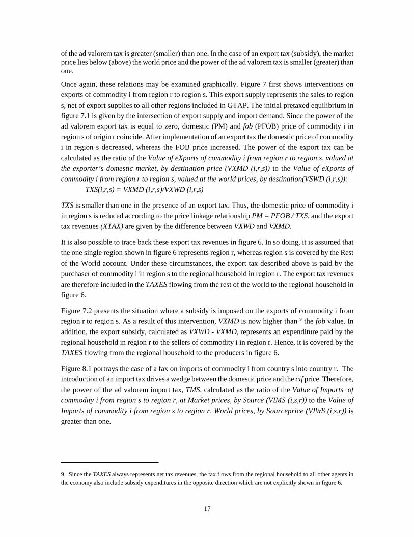
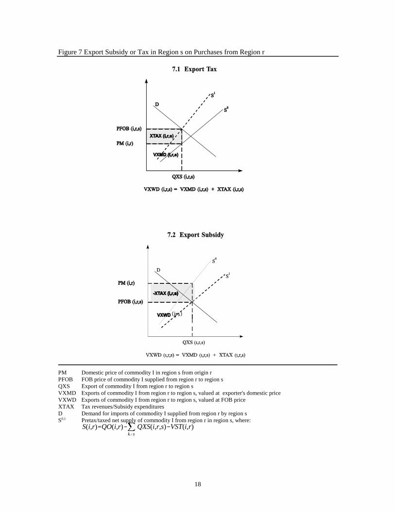
Once again, these relations may be examined graphically. Figure 7 first shows interventions on
exports of commodity i from region r to region s. This export supply represents the sales to region
s, net of export supplies to all other regions included in GTAP. The initial pretaxed equilibrium in
figure 7.1 is given by the intersection of export supply and import demand. Since the power of the
ad valorem export tax is equal to zero, domestic (PM) and fob (PFOB) price of commodity i in
region s of origin r coincide. After implementation of an export tax the domestic price of commodity
i in region s decreased, whereas the FOB price increased. The power of the export tax can be
calculated as the ratio of the Value of eXports of commodity i from region r to region s, valued at
the exporter’s domestic market, by destination price (VXMD (i,r,s)) to the Value of eXports of
commodity i from region r to region s, valued at the world prices, by destination(VSWD (i,r,s)):
TXS(i,r,s) = VXMD (i,r,s)/VXWD (i,r,s)
TXS is smaller than one in the presence of an export tax. Thus, the domestic price of commodity i
in region s is reduced according to the price linkage relationship PM = PFOB / TXS, and the export
tax revenues (XTAX) are given by the difference between VXWD and VXMD.
It is also possible to trace back these export tax revenues in figure 6. In so doing, it is assumed that
the one single region shown in figure 6 represents region r, whereas region s is covered by the Rest
of the World account. Under these circumstances, the export tax described above is paid by the
purchaser of commodity i in region s to the regional household in region r. The export tax revenues
are therefore included in the TAXES flowing from the rest of the world to the regional household in
figure 6.
Figure 7.2 presents the situation where a subsidy is imposed on the exports of commodity i from
region r to region s. As a result of this intervention, VXMD is now higher than 9 the fob value. In
addition, the export subsidy, calculated as VXWD - VXMD, represents an expenditure paid by the
regional household in region r to the sellers of commodity i in region r. Hence, it is covered by the
TAXES flowing from the regional household to the producers in figure 6.
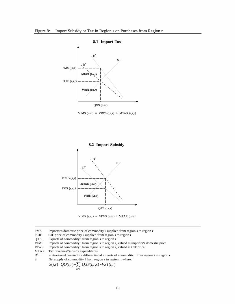
Figure 8.1 portrays the case of a fax on imports of commodity i from country s into country r. The
introduction of an import tax drives a wedge between the domestic price and the cif price. Therefore,
the power of the ad valorem import tax, TMS, calculated as the ratio of the Value of Imports of
commodity i from region s to region r, at Market prices, by Source (VIMS (i,s,r)) to the Value of
Imports of commodity i from region s to region r, World prices, by Sourceprice (VIWS (i,s,r)) is
greater than one.
18
(irs)
Figure 7 Export Subsidy or Tax in Region s on Purchases from Region r
PM Domestic price of commodity I in region s from origin rPFOB FOB price of commodity I supplied from region r to region sQXS Export of commodity I from region r to region sVXMD Exports of commodity I from region r to region s, valued at exporter's domestic priceVXWD Exports of commodity I from region r to region s, valued at FOB priceXTAX Tax revenues/Subsidy expendituresD Demand for imports of commodity I supplied from region r by region sS0,1 Pretax/taxed net supply of commodity I from region r in region s, where:
S(i,r)�QO(i,r)��k�s
QXS(i,r,s)�VST(i,r)
19
S(i,r)�QO(i,r)��k�s
QXS(i,r,s)�VST(i,r)
Figure 8: Import Subsidy or Tax in Region s on Purchases from Region r
PMS Importer's domestic price of commodity i supplied from region s to region rPCIF CIF price of commodity i supplied from region s to region rQXS Exports of commodity i from region s to region rVIMS Imports of commodity i from region s to region r, valued at importer's domestic priceVIWS Imports of commodity i from region s to region r, valued at CIF priceMTAX Tax revenues/Subsidy expendituresD0,1 Pretax/taxed demand for differentiated imports of commodity i from region s in region rS Net supply of commodity I from region s in region r, where:
20
Given the price linkage relationship PMS = PCIF / TMS, the import tax revenues can be computedas follows:
MTAX (i,s,r) = VIMS (i,s,r) - VIWS (i,s,r)
These import taxes are paid by the purchaser of commodity i (private household, government and
firms) in region r. Since tax revenues always accrue to the regional household these import taxes are
included in the TAXES flowing from the private household, the government and the producers to the
regional household in region r (figure 6).
Finally, figure 8.2 demonstrates the situation which results in the presence of an import subsidy.
Here, the cif price of commodity i supplied from region s to region r exceeds the importer’s domestic
price. Accordingly, the power of the ad valorem import tax is smaller than one, and MTAX calculated
as the difference between VIMS and VIWS is an expenditure that is withdrawn from the regional
household. In figure 6, import subsidy expenditures are embodied in the TAXES flowing from the
regional household to all purchases of imported commodity i. Since this value flow is the last one
to be considered, it also completes the overview of the basic structure of GTAP. Readers wishing
to continue their introduction to the GTAP model are referred to chapter 2 of the GTAP book
(HERTEL, ed.)
21
References
HERTEL, T.W., PETERSEN, E.B., PRECKEL, P., SURRY. Y. and TIGAS, M.E. (1991), “Implicitadditivity as a strategy for restricting the parameter space in CGE models,” Economic andFinancial Computing, Vol. 1, No. 1, pp. 265-289.
HERTEL, T.W. (ed.), Global Trade Analysis Project: Modeling and Applications. CambridgeUniversity Press, 1997.
MCDOUGALL, R. A., (2001), “A New Regional Household Demand System for GTAP,” GTAPTechnical Paper No. 20, Center for Global Trade Analysis, Purdue University,http://www.gtap.org.