A Gravity Model of Sovereign Lending: Trade, Default and Credit

Andrew K. Rose and Mark M. Spiegel*

Draft: December 3, 2003

Abstract One reason why countries service their external debts is the fear that default might lead to shrinkage of international trade. If so, then creditors should systematically lend more to countries with which they share closer trade links. We develop a simple theoretical model to capture this intuition, then test and corroborate this idea. Keywords : panel, bilateral, bank, loan, sovereign risk JEL Classification Numbers : F15, F33 Andrew K. Rose (correspondence) Mark M. Spiegel Haas School of Business Federal Reserve Bank of San Francisco University of California 101 Market St. Berkeley, CA USA 94720-1900 San Francisco CA 94105 Tel: (510) 642-6609 Tel: (415) 974-3241 Fax: (510) 642-4700 Fax: (415) 974-2168 E-mail: arose@haas.berkeley.edu E-mail: mark.spiegel@sf.frb.org * Rose is B.T. Rocca Jr. Professor of International Trade and Economic Analysis and Policy in the Haas School of Business at the University of California, Berkeley, NBER research associate and CEPR Research Fellow. Spiegel is Senior Research Advisor, Economic Research Department, Federal Reserve Bank of San Francisco. We thank Rob Feenstra for a comment which helped inspire this paper; Rose thanks INSEAD for hospitality while part of this paper was written. We also thank Gerd Haeusler, Phillip Lane, Nancy Marion, Paulo Mauro, Michael Mussa, and participants at ARC-4 at the IMF and especially Mark Wright for comments. The views expressed below do not represent those of the Federal Reserve Bank of San Francisco or the Board of Governors of the Federal Reserve System, or their staffs. A current (PDF) version of this paper and the STATA data set used in the paper are available at http://faculty.haas.berkeley.edu/arose.

1

1: Introduction

While the age of gunboat diplomacy as a mechanism of credit enforcement has long

passed, sovereign default is still an exceptional event. This stylized fact indicates that while the

source of a sovereign default penalty is still controversial, sovereigns behave as if they consider

default costly. Many models of sovereign debt in the literature [e.g. Bulow and Rogoff (1989a),

(1989b)] introduce explicit default penalties to rationalize this fact. These sanctions are

primarily considered to be methods of inhibiting trade. Bulow and Rogoff (1989a) discuss the

difficulties countries would experience in their trade subsequent to default, including

complications associated with avoiding seizure and the interruption of short-term trade credit.

Nevertheless, there are a number of reasons why one might doubt the existence of default

penalties. Bulow and Rogoff (1989b) themselves admit that it is unclear whether private

creditors enjoy the ability to induce their governments to enforce claims on sovereign borrowers.

Kletzer and Wright (2000) argue that most penalties in models of sovereign lending are not

“renegotiation-proof.” That is, Kletzer and Wright argue that both parties could do better

subsequent to a full or partial sovereign default, if the creditor resists levying a destructive

penalty from which (s)he would receive no immediate benefit. In brief, there is considerable

uncertainty concerning the viability of penalties for sovereign default. Thus, empirical evidence

regarding such penalties warrants attention.

Unfortunately, there are only a limited number of empirical studies concerning such

penalties. Ozler (1993) provides evidence of positive, albeit small, premia charged to countries

with default histories. Cline (1987) notes that Bolivia and Peru experienced interruptions in their

flows of short-term trade credits subsequent to debt renegotiation. In a recent paper, Rose (2002)

provides empirical support for the role of trade as a sovereign enforcement mechanism. His

2

paper shows that sovereign Paris Club reschedulings are followed by economically and

statistically significant reductions in international trade.

The evidence of Cline and Rose centers on the interruption of international trade as a

mechanism for sovereign debt repayment. If one believes that the primary penalties for

enforcing sovereign debt obligations are trade related, then creditors originating from nations

with strong bilateral trade ties with a debtor nation should have a comparative advantage in

lending to that nation.

In this short paper, we explore this idea. We first present a theoretical model of

international lending where a debtor optimally chooses its borrowing from different creditors.

These creditors are identical except that they are located in countries which differ by the strength

of their bilateral trade ties with the debtor. We show that in equilibrium, the pattern of

borrowing favors the creditor with higher bilateral trade volume with the debtor. We then test

and corroborate this idea using an annual panel data set including bilateral trade and international

banking claims from 20 creditor and 149 debtor countries from 1986 through 1999. Using

instrumental variable (and other) techniques, we find a significantly positive effect of bilateral

trade on bilateral lending patterns. That is, debtors tend to borrow more from creditors with

whom they share more international trade ties.

While our empirical results support the trade sanction sovereign debt model derived in

the paper, the evidence does not necessarily refute pure “reputation-based” models of sovereign

debt in which the penalty for default is exclusion from access to future borrowing [e.g. Eaton and

Gersovitz (1981), Kletzer and Wright (2000), or Wright (2002)], or with mixed models where

some combination of direct sanctions and reputational penalties are applied, such as Kehoe and

Levine (1993).1 However, it appears that reconciling reputation-based models with the data

3

without introducing new inconsistencies requires the introduction of some friction, such as

superior information sets to creditors from those countries engaged in greater bilateral trade.2

Our theoretical model is presented in next section. We then present the data set and

methodology and test the model. The paper ends with a brief summary.

2: A Model of Sovereign Borrowing with Trade-Related Default Penalties

In this section we develop a simple borrowing model in which a sovereign debtor

allocates its borrowing across different creditor nations, when default penalties are based on

proportional losses in bilateral gains from trade.

We assume that there are three countries: one borrower country, i, and two creditor

countries, a and b. Let r represent one plus the world risk-free interest rate. All countries are

assumed to be small and therefore take r as given. Lending banks in the creditor countries are

risk-neutral and therefore willing to extend unlimited funds at levels consistent with an expected

return equal to r.

The model has two periods. In the first period, the representative agent in lender country j

(j=a,b) extends a loan of magnitude ijL in return for the promise of a fixed payment ijD in the

second period. In the second period, the agent in debtor country i makes its default decisions. If

the debtor chooses to service its country j debt it pays ijD . If the debtor defaults, it suffers a

penalty equal to a fraction θ of its gains from bilateral trade with country j, where 0 1.θ< <

Bilateral gains from trade are exogenous and equal to ijTγ , where ? is a positive constant

and ijT is a random variable reflecting total trade between country i and country j in the second

period. Expectations of ijT are unbiased and satisfy

4

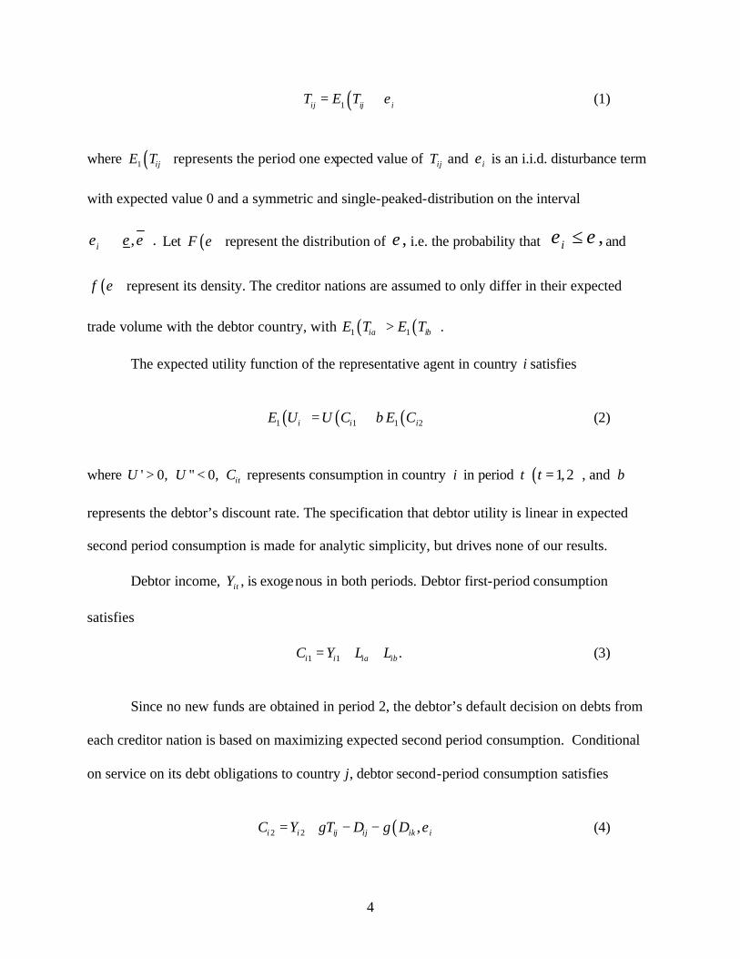
( )1ij ij iT E T ε= + (1)

where ( )1 ijE T represents the period one expected value of ijT and iε is an i.i.d. disturbance term

with expected value 0 and a symmetric and single-peaked-distribution on the interval

, .iε ε ε ∈ Let ( )F ε represent the distribution of ,ε i.e. the probability that ,iε ε≤ and

( )f ε represent its density. The creditor nations are assumed to only differ in their expected

trade volume with the debtor country, with ( ) ( )1 1ia ibE T E T> .

The expected utility function of the representative agent in country i satisfies

( ) ( ) ( )1 1 1 2i i iE U U C E Cβ= + (2)

where ' 0,U > " 0,U < itC represents consumption in country i in period t ( )1,2t = , and β

represents the debtor’s discount rate. The specification that debtor utility is linear in expected

second period consumption is made for analytic simplicity, but drives none of our results.

Debtor income, itY , is exogenous in both periods. Debtor first-period consumption

satisfies

1 1 .i i ia ibC Y L L= + + (3)

Since no new funds are obtained in period 2, the debtor’s default decision on debts from

each creditor nation is based on maximizing expected second period consumption. Conditional

on service on its debt obligations to country j, debtor second-period consumption satisfies

( )2 2 ,i i ij ij ik iC Y T D g Dγ ε= + − − (4)

5

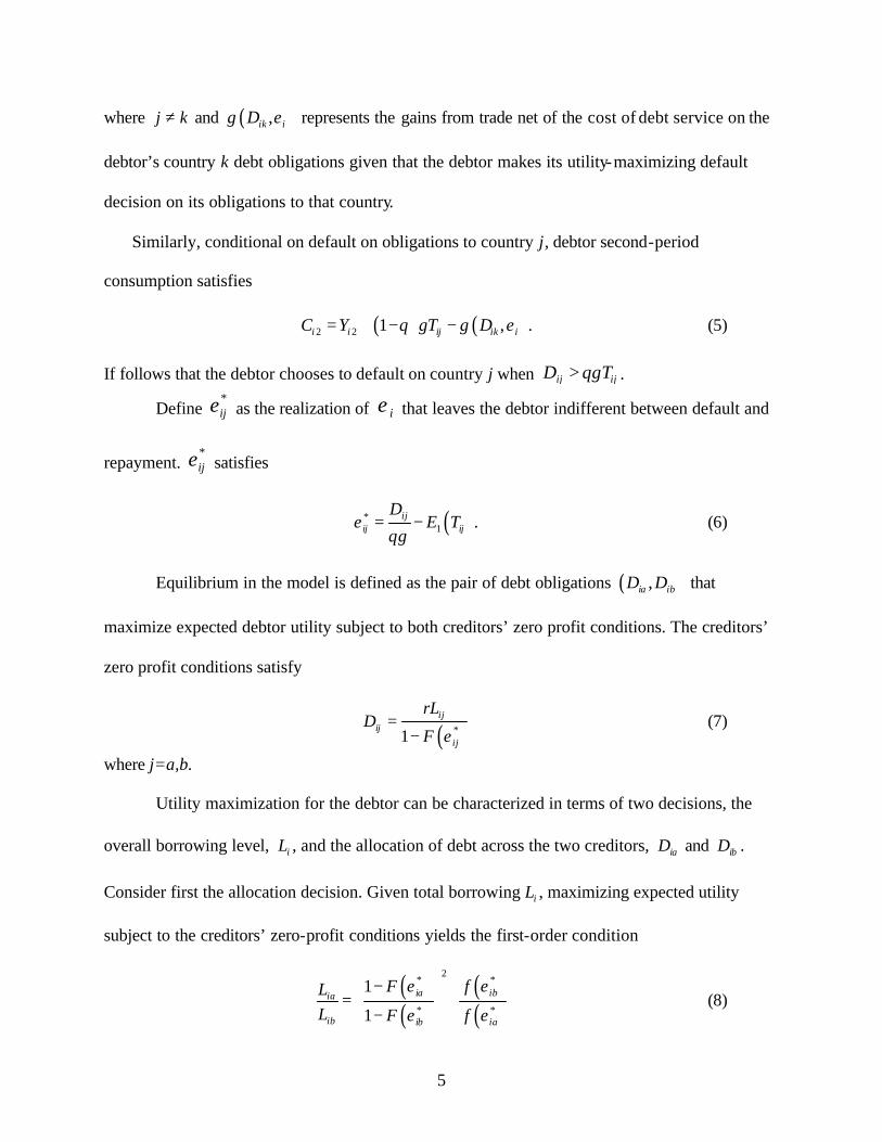
where j k≠ and ( ),ik ig D ε represents the gains from trade net of the cost of debt service on the

debtor’s country k debt obligations given that the debtor makes its utility-maximizing default

decision on its obligations to that country.

Similarly, conditional on default on obligations to country j, debtor second-period

consumption satisfies

( ) ( )2 2 1 , .i i ij ik iC Y T g Dθ γ ε= + − − (5) If follows that the debtor chooses to default on country j when ij ijD Tθγ> .

Define *ijε as the realization of iε that leaves the debtor indifferent between default and

repayment. *ijε satisfies

( )*1 .ij

ij ij

DE Tε

θγ= − (6)

Equilibrium in the model is defined as the pair of debt obligations ( ),ia ibD D that

maximize expected debtor utility subject to both creditors’ zero profit conditions. The creditors’

zero profit conditions satisfy

( )*1ij

ijij

rLD

F ε=

− (7)

where j=a,b.

Utility maximization for the debtor can be characterized in terms of two decisions, the

overall borrowing level, iL , and the allocation of debt across the two creditors, iaD and ibD .

Consider first the allocation decision. Given total borrowing iL , maximizing expected utility

subject to the creditors’ zero-profit conditions yields the first-order condition

( )( )

( )( )

2* *

* *

1

1ia ibia

ib ib ia

F fLL F f

ε ε

ε ε

− = −

(8)

6

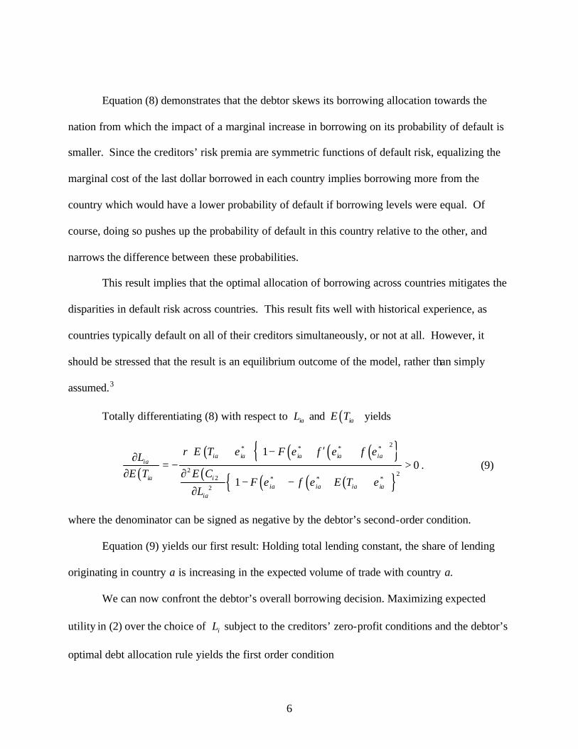
Equation (8) demonstrates that the debtor skews its borrowing allocation towards the

nation from which the impact of a marginal increase in borrowing on its probability of default is

smaller. Since the creditors’ risk premia are symmetric functions of default risk, equalizing the

marginal cost of the last dollar borrowed in each country implies borrowing more from the

country which would have a lower probability of default if borrowing levels were equal. Of

course, doing so pushes up the probability of default in this country relative to the other, and

narrows the difference between these probabilities.

This result implies that the optimal allocation of borrowing across countries mitigates the

disparities in default risk across countries. This result fits well with historical experience, as

countries typically default on all of their creditors simultaneously, or not at all. However, it

should be stressed that the result is an equilibrium outcome of the model, rather than simply

assumed.3

Totally differentiating (8) with respect to iaL and ( )iaE T yields

( )

( ) ( ) ( ) ( ){ }( ) ( ) ( ) ( ){ }

2* * * *

2 22 * * *

2

10

1

ia ia ia ia iaia

ia iia ia ia ia

ia

r E T F f fLE T E C

F f E TL

ε ε ε ε

ε ε ε

′ + − + ∂= − >

∂ ∂ − − + ∂

. (9)

where the denominator can be signed as negative by the debtor’s second-order condition.

Equation (9) yields our first result: Holding total lending constant, the share of lending

originating in country a is increasing in the expected volume of trade with country a.

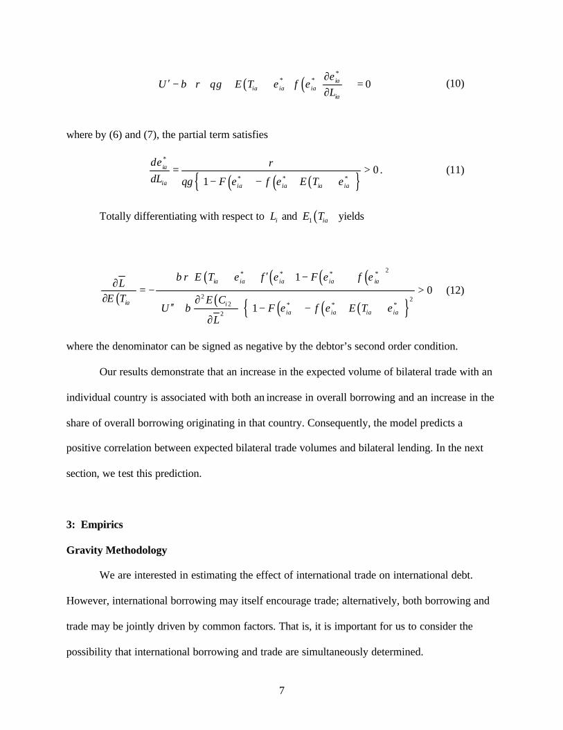
We can now confront the debtor’s overall borrowing decision. Maximizing expected

utility in (2) over the choice of iL subject to the creditors’ zero-profit conditions and the debtor’s

optimal debt allocation rule yields the first order condition

7

( ) ( )*

* * 0iaia ia ia

ia

U r E T fLε

β θγ ε ε ∂ ′ − + + = ∂

(10)

where by (6) and (7), the partial term satisfies

( ) ( ) ( ){ }

*

* * *0

1ia

ia ia ia ia ia

d rdL F f E T

ε

θγ ε ε ε= >

− − +

. (11)

Totally differentiating with respect to iL and ( )1 iaE T yields

( )( ) ( ) ( ) ( )

( ) ( ) ( ) ( ){ }

2* * * *

2 22 * * *

2

10

1

ia ia ia ia ia

ia iia ia ia ia

r E T f F fLE T E C

U F f E TL

β ε ε ε ε

β ε ε ε

′ + − + ∂ = − >∂ ∂

′′ + − − + ∂

(12)

where the denominator can be signed as negative by the debtor’s second order condition.

Our results demonstrate that an increase in the expected volume of bilateral trade with an

individual country is associated with both an increase in overall borrowing and an increase in the

share of overall borrowing originating in that country. Consequently, the model predicts a

positive correlation between expected bilateral trade volumes and bilateral lending. In the next

section, we test this prediction.

3: Empirics

Gravity Methodology

We are interested in estimating the effect of international trade on international debt.

However, international borrowing may itself encourage trade; alternatively, both borrowing and

trade may be jointly driven by common factors. That is, it is important for us to consider the

possibility that international borrowing and trade are simultaneously determined.

8

We solve this problem using instrumental variables. The popular “gravity” model of

bilateral international trade provides a wealth of potential instrumental variables. Many variables

which are known to be important determinants of international trade are unlikely to be important

determinants of international lending patterns. For instance, a pair of landlocked countries

engages in less international trade, while a pair of physically large countries or those which share

a common land border trade more. But international lending patterns are unlikely to be affected

by such features.4 We use such variables as instrumental variables for trade in a model of

bilateral lending.

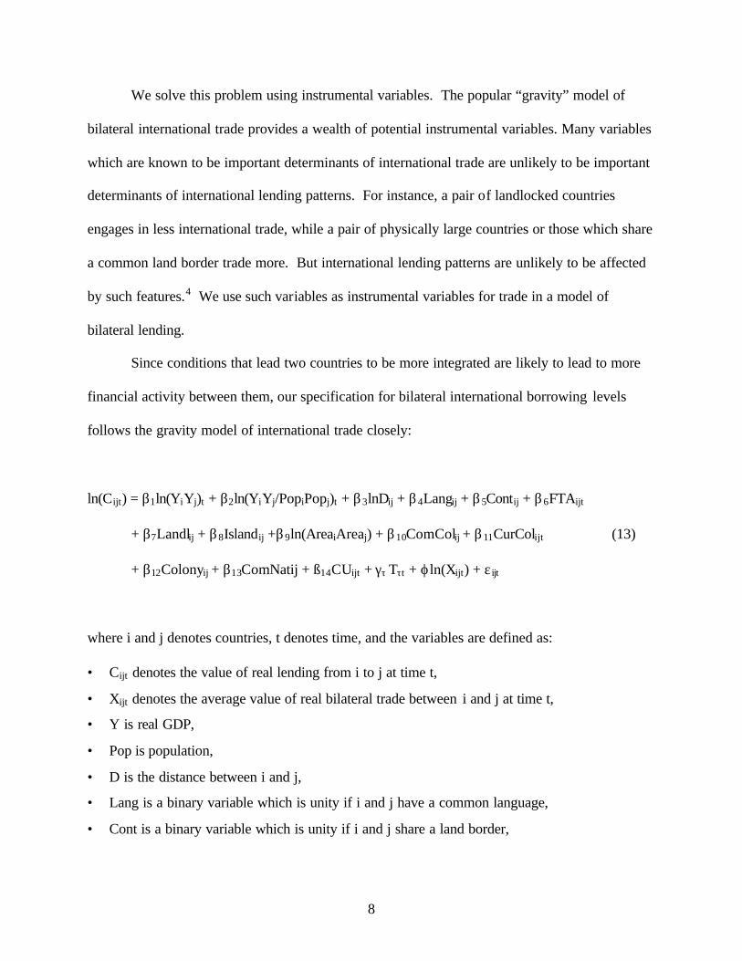
Since conditions that lead two countries to be more integrated are likely to lead to more

financial activity between them, our specification for bilateral international borrowing levels

follows the gravity model of international trade closely:

ln(Cijt) = β1ln(YiYj)t + β2ln(YiYj/PopiPopj)t + β3lnDij + β4Langij + β5Contij + β6FTAijt

+ β7Landlij + β8Islandij +β9ln(AreaiAreaj) + β10ComColij + β11CurColijt (13)

+ β12Colonyij + β13ComNatij + ß14CUijt + γτ⋅Tτt + ϕln(Xijt) + ε ijt

where i and j denotes countries, t denotes time, and the variables are defined as: • Cijt denotes the value of real lending from i to j at time t,

• Xijt denotes the average value of real bilateral trade between i and j at time t,

• Y is real GDP,

• Pop is population,

• D is the distance between i and j,

• Lang is a binary variable which is unity if i and j have a common language,

• Cont is a binary variable which is unity if i and j share a land border,

9

• FTA is a binary variable which is unity if i and j belong to the same regional trade

agreement,

• Landl is the number of landlocked countries in the country-pair (0, 1, or 2).

• Island is the number of island nations in the pair (0, 1, or 2),

• Area is the land mass of the country,

• ComCol is a binary variable which is unity if i and j were ever colonies after 1945 with the

same colonizer,

• CurCol is a binary variable which is unity if i and j are colonies at time t,

• Colony is a binary variable which is unity if i ever colonized j or vice versa,

• ComNat is a binary variable which is unity if i and j remained part of the same nation during

the sample (e.g., the UK and Bermuda),

• CU is a binary variable which is unity if i and j use the same currency at time t,

• Tτt is a comprehensive set of year-specific intercepts,

• β and γ are vectors of nuisance coefficients, and

• ε ij represents the myriad other influences on bilateral credit, assumed to be well behaved.

The coefficient of interest to us is ϕ, the effect of bilateral trade between countries i and j on

commercial bank claims by creditor country j on debtor nation i.

We estimate the model with a number of techniques below. We begin by using ordinary least

squares with standard errors that are robust to clustering (since pairs of countries are likely to be

highly dependent across years). We then use instrumental variables, dropping some of the

regressors from the right-hand side of the equation and using them as instrumental variables.

Finally, we employ fixed- and random-effects panel data estimators, with and without

instrumental variables. We use both fixed and random effects estimators extensively below.

The Data Set

10

We use a subset of the panel data set of Glick and Rose (2002); the interested reader is

referred to Glick and Rose for more details.

For the regressand we use consolidated foreign claims of reporting banks on individual

countries.5 These bank loans are provided by the BIS in millions of American dollars for twenty

creditor countries and almost 150 borrowing countries.6 Not all of the areas covered are

countries in the conventional sense of the word; we use the term “country” simply for

convenience. (The creditor countries and debtor countries are listed in the appendix.) The data

are provided semi-annually from 1986; we average the data to annual series by simple averaging.

We convert nominal bank claims to a real series by deflating by the American CPI (1982-

1984=1). Almost half the claims are reported to be zero. This makes the log transformation

potentially important and questionable; we investigate it further below.

The most important regressor is the level of international trade. We use bilateral trade

flows taken from the IMF’s Direction of Trade data set, deflated by the American CPI.7 To this

we add population and real GDP data (in constant dollars).8 We exploit the CIA’s “World

Factbook” for a number of country-specific variables. These include: latitude and longitude, land

area, landlocked and island status, physically contiguous neighbors, language, colonizers, and

dates of independence. We use these to create great-circle distance and our other controls. We

obtain data from the World Trade Organization to create an indicator of regional trade

agreements, and include: EEC/EC/EU; US-Israel FTA; NAFTA; CACM; CARICOM;

PATCRA; ANZCERTA; ASEAN, SPARTECA, and Mercosur. Finally, we add the Glick and

Rose (2002) currency union dummy variable.

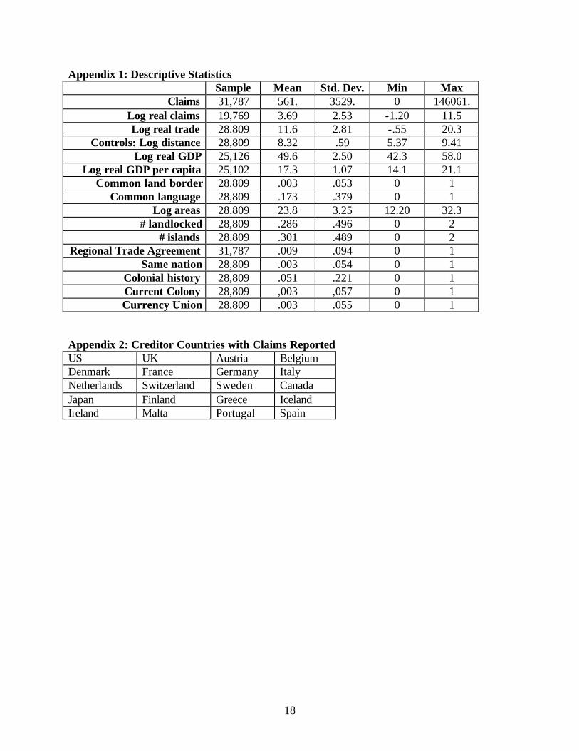
Descriptive statistics for the data set are tabulated in the appendix.

11

Results

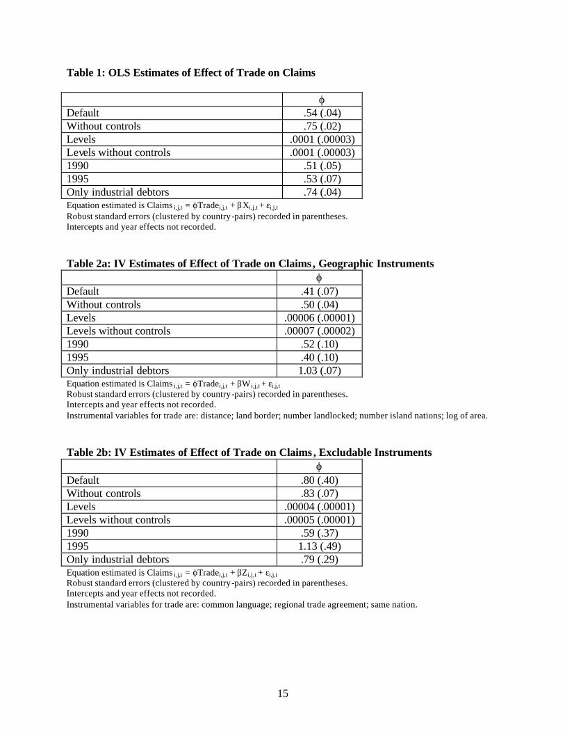
We begin our investigation by estimating (14) with OLS. Our results appear in Table 1.

Our default estimates include the entire set of regressors (i.e., all fourteen coefficients are

estimated as well as the set of time-specific intercepts). In this specification, the estimate of the

all- important ϕ coefficient is .54, with a robust standard error of .04. This elasticity is not only

consistent with our theory, but is highly significant. With a t-statistic of over 15, the coefficient

is different from zero at any reasonable level of statistical significance. The effect is also

economically significant; an increase in trade of 1% is associated with an increase in bilateral

lending of over .5%, all other things being equal. Of course, since there are capital flows above

and beyond the bank lending that we consider (through e.g., stock and bond markets, as well as

foreign direct investment), even this considerable elasticity should probably be considered a

lower bound.

The rest of the table provides a series of robustness checks. For instance, the second row

reports ϕ if the other controls are dropped from the equation (i.e., we set β =γ=0); in this case, the

effect is even more significant. Since many of the creditor countries have not extended loans to

some of the debtor countries, many observations of the dependent variable are zero and are thus

dropped from the equation estimated in natural logarithms. Therefore, the third and fourth rows

of the table report comparable estimates of ϕ when both trade and bank claims are included in

untransformed levels. Yet ϕ remains statistically significant when the key relationship is

estimated in levels.9

The fifth and sixth rows of the table move away from panel data analysis to cover only

cross-sections for two years in the middle of the sample, 1990 and 1995. However, the results

are essentially unchanged from the default specification. The seventh and final row includes

12

only observations between industrial countries (i.e., those with IFS country codes less than 200).

If anything, the results become mysteriously larger; they certainly remain positive and highly

significant in both the economic and statistical senses.10

To summarize, the effect of international trade on bank claims seems positive,

significant, and robust in simple OLS estimation. The question is whether this result stands up to

greater econometric scrutiny.

IV Results

We now proceed to instrumental variables estimation. We use five instrumental variables

for (the log of) trade: (the log of) distance between the countries; the land border dummy; the

number of landlocked countries; the number of island nations; and the log of the product of the

countries’ area. We accordingly set the appropriate β coefficients to zero (i.e., drop them from

the equation, leaving the remaining variables as controls). The estimates are tabulated in Table

2a.

Despite the use of instrumental variables that are both plausibly exogenous and correlated

with trade, the key results do not change with IV estimation. The default estimate is somewhat

smaller, averaging perhaps .4. But it remains economically and statistically significant; it is also

robust to a number of econometric perturbations.11

Table 2b reports sensitivity analysis with respect to the set of instrumental variables.

Instead of the five geographic variables, we use three whose coefficients are usually insignificant

in OLS estimates of equation (14): the common language dummy; the regional trade agreement

dummy; and the same nation dummy. Again, the estimates of ϕ seem economically and

statistically significant.12

13

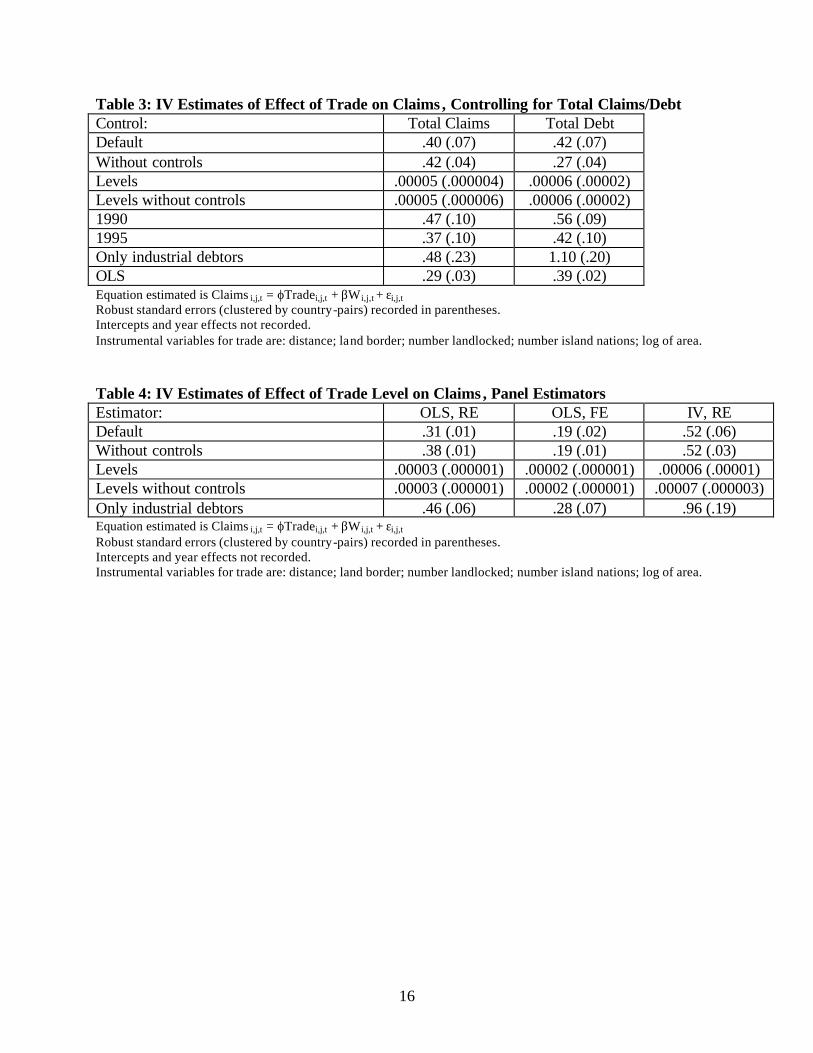
The middle column of Table 3 adds a control for the (log of the) total credit extended by

the creditor country, as suggested by our theoretical analysis; the right-hand column controls for

the (log of) total debt incurred by the debtor country. Again, the results remain economically

and statistically significant.

Finally, Table 4 reports results when panel estimators are used instead of more traditional

regressions. The middle columns report OLS fixed- and random-effects estimates of ϕ for a

variety of different specifications. The former takes into account all country-pair factors that

influence trade whether measured or not, and is thus an exceptionally good robustness check.

The right-hand column reports instrumental variables estimates using a random effects estimator

(the fixed-effect estimator is infeasible since the geographic variables are time- invariant). Yet

despite all the econometric firepower, the estimate of ϕ remains significant; it has a t-statistic of

almost 9 and an economically large effect.13

We conclude that our hypothesis that bank credit is extended across international borders

along the lines of international trade is corroborated.

4: Summary

It is plausible to believe that countries service their foreign debts at least in part to avoid

the reduced trade that typically follows international default. If so, sovereign borrowers will

enjoy superior credit terms from creditor countries for which this penalty is disproportionately

high. In this paper we have provided a simple theoretical model which formalizes this intuition.

We have also empirically investigated and confirmed the hypothesis that international trade

patterns determine lending patterns.

14

In future work it would be interesting to extend this analysis to other forms of

international lending, above and beyond bank loans. We think this is a good place to pass the

torch to others.

15

Table 1: OLS Estimates of Effect of Trade on Claims

ϕ Default .54 (.04) Without controls .75 (.02) Levels .0001 (.00003) Levels without controls .0001 (.00003) 1990 .51 (.05) 1995 .53 (.07) Only industrial debtors .74 (.04) Equation estimated is Claims i,j,t = ϕTradei,j,t + βXi,j,t + εi,j,t Robust standard errors (clustered by country-pairs) recorded in parentheses. Intercepts and year effects not recorded. Table 2a: IV Estimates of Effect of Trade on Claims , Geographic Instruments ϕ Default .41 (.07) Without controls .50 (.04) Levels .00006 (.00001) Levels without controls .00007 (.00002) 1990 .52 (.10) 1995 .40 (.10) Only industrial debtors 1.03 (.07) Equation estimated is Claims i,j,t = ϕTradei,j,t + βWi,j,t + εi,j,t Robust standard errors (clustered by country-pairs) recorded in parentheses. Intercepts and year effects not recorded. Instrumental variables for trade are: distance; land border; number landlocked; number island nations; log of area. Table 2b: IV Estimates of Effect of Trade on Claims , Excludable Instruments ϕ Default .80 (.40) Without controls .83 (.07) Levels .00004 (.00001) Levels without controls .00005 (.00001) 1990 .59 (.37) 1995 1.13 (.49) Only industrial debtors .79 (.29) Equation estimated is Claims i,j,t = ϕTradei,j,t + βZi,j,t + εi,j,t Robust standard errors (clustered by country-pairs) recorded in parentheses. Intercepts and year effects not recorded. Instrumental variables for trade are: common language; regional trade agreement; same nation.

16

Table 3: IV Estimates of Effect of Trade on Claims , Controlling for Total Claims/Debt Control: Total Claims Total Debt Default .40 (.07) .42 (.07) Without controls .42 (.04) .27 (.04) Levels .00005 (.000004) .00006 (.00002) Levels without controls .00005 (.000006) .00006 (.00002) 1990 .47 (.10) .56 (.09) 1995 .37 (.10) .42 (.10) Only industrial debtors .48 (.23) 1.10 (.20) OLS .29 (.03) .39 (.02) Equation estimated is Claims i,j,t = ϕTradei,j,t + βWi,j,t + εi,j,t Robust standard errors (clustered by country-pairs) recorded in parentheses. Intercepts and year effects not recorded. Instrumental variables for trade are: distance; land border; number landlocked; number island nations; log of area. Table 4: IV Estimates of Effect of Trade Level on Claims , Panel Estimators Estimator: OLS, RE OLS, FE IV, RE Default .31 (.01) .19 (.02) .52 (.06) Without controls .38 (.01) .19 (.01) .52 (.03) Levels .00003 (.000001) .00002 (.000001) .00006 (.00001) Levels without controls .00003 (.000001) .00002 (.000001) .00007 (.000003) Only industrial debtors .46 (.06) .28 (.07) .96 (.19) Equation estimated is Claims i,j,t = ϕTradei,j,t + βWi,j,t + εi,j,t Robust standard errors (clustered by country-pairs) recorded in parentheses. Intercepts and year effects not recorded. Instrumental variables for trade are: distance; land border; number landlocked; number island nations; log of area.

17

References Bulow, Jeremy and Kenneth Rogoff (1989a) “A Constant Recontracting Model of Sovereign Debt” Journal of Political Economy 97(1), 155-178. Bulow, Jeremy and Kenneth Rogoff (1989b) “Sovereign Debt: Is to Forgive to Forget?” American Economic Review 79(1), 43-50. Cline, William R. (1987) Mobilizing Bank Lending to Debtor Countries, Institute for International Economics, Washington D.C. Glick, Reuven and Andrew K. Rose (2002) “Does a Currency Union Affect Trade?” European Economic Review forthcoming. Kehoe, Timothy J. and David K. Levine (1993) “Debt-Constrained Asset Markets,” Review of Economis Studies 60, 865-888. Kletzer, Kenneth M. and Brian D. Wright (2000) “Sovereign Debt as Intertemporal Barter” American Economic Review 90(3), 621-639. Wright, Mark L. J. (2002) “Reputations and Sovereign Debt” mimeo, Stanford University. Wright, Mark L. J. (2004) “Discussion of ‘A Gravity Model of Sovereign Lending: Trade Default and Credit’” forthcoming, International Monetary Fund Staff Papers. Ozler, Sule (1993) “Have Commercial Banks Ignored History?” American Economic Review 83(3), 608-620. Rose, Andrew K. (2002) “One Reason Countries Pay Their Debts: Renegotiation and International Trade” NBER Working Paper 8853.

18

Appendix 1: Descriptive Statistics Sample Mean Std. Dev. Min Max

Claims 31,787 561. 3529. 0 146061. Log real claims 19,769 3.69 2.53 -1.20 11.5 Log real trade 28.809 11.6 2.81 -.55 20.3

Controls: Log distance 28,809 8.32 .59 5.37 9.41 Log real GDP 25,126 49.6 2.50 42.3 58.0

Log real GDP per capita 25,102 17.3 1.07 14.1 21.1 Common land border 28.809 .003 .053 0 1

Common language 28,809 .173 .379 0 1 Log areas 28,809 23.8 3.25 12.20 32.3

# landlocked 28,809 .286 .496 0 2 # islands 28,809 .301 .489 0 2

Regional Trade Agreement 31,787 .009 .094 0 1 Same nation 28,809 .003 .054 0 1

Colonial history 28,809 .051 .221 0 1 Current Colony 28,809 ,003 ,057 0 1 Currency Union 28,809 .003 .055 0 1

Appendix 2: Creditor Countries with Claims Reported US UK Austria Belgium Denmark France Germany Italy Netherlands Switzerland Sweden Canada Japan Finland Greece Iceland Ireland Malta Portugal Spain

19

Appendix 3: Debtor Countries with Claims Reported Afghanistan Ghana Nigeria Albania Gibraltar Oman Algeria Greece Pakistan Angola Grenada Panama Argentina Guatemala Papua New Guinea Australia Guinea Paraguay Bahamas Guinea Bissau Peru Bahrain Guyana Philippines Bangladesh Haiti Poland Barbados Honduras Portugal Belize Hong Kong Qatar Benin Hungary Romania Bermuda Iceland Rwanda Bhutan India Sao Tome and Principe Bolivia Indonesia Saudi Arabia Botswana Iran Senegal Brazil Iraq Seychelles Brunei Israel Sierra Leone Bulgaria Jamaica Singapore Burkina Faso Jordan Solomon Islands Burundi Kenya Somalia Cambodia Kiribati South Africa Cameroon Kuwait South Korea Cape Verde Laos Sri Lanka Cayman Islands Lebanon St Lucia Central African Rep. Lesotho St Vincent Chad Liberia St Helena Chile Libya Sudan China Macau Surinam Colombia Madagascar Swaziland Comoros Islands Malawi Syria Congo Malaysia Tanzania Congo Democratic Republic Maldives Thailand Costa Rica Mali Togo Cote d'Ivoire Malta Tonga Cuba Mauritania Trinidad and Tobago Cyprus Mauritius Tunisia Djibouti Mexico Turkey Dominica Mongolia Uganda Dominican Republic Morocco United Arab Emirates Ecuador Mozambique Uruguay Egypt Myanmar Vanuatu El Salvador Namibia Venezuela Equatorial Guinea Nauru Vietnam Ethiopia Nepal Western Samoa Falkland Islands Netherlands Antilles Yemen Fiji New Caledonia Yugoslavia French Polynesia New Zealand Zambia Gabon Nicaragua Zimbabwe Gambia Niger

20

Endnotes 1 While the Kehoe and Levine model allows for asset seizure, it does not consider interruptions of trade in spot

markets, which might be considered analogous to the direct trade sanctions in our model below. 2 See Wright’s (2004) comments on our paper below. Wright argues that the assumption of superior information

sets held by primary trading partners may give those partners comparative advantages in lending in pure reputation

models with the additional assumption of continuous trade in goods to avoid the “excessive gross flows” problem.

3 In the limiting case where the 'ij sε are distributed uniform, the equilibrium borrowing allocation results in the

debtor defaulting on both creditors or none. 4 If bank lending reflects trade credits, coefficient estimates from our IV estimation may be biased upwards.

However, as our estimated effect is large, it is unlikely that correction for this bias would eliminate our results. 5 Our measurement of cross-border obligations may contain errors from a number of sources. First, the use of

consolidated data may not correctly assign the risk of banks’ foreign-branches. Second, “outward risk transfers” are

sometimes used to transfer risks to residents of other countries, and our data set would not pick these up. Still, as

these errors fall in the regressand of our model they only make the effect of trade harder to find and do not appear to

introduce any bias issues. 6 These data are available at: http://www.bis.org/publ/qcsv0206/hanx9b.csv and are part of the International

Banking Statistics published regularly in the BIS Quarterly Review. For technical reasons we usually ignore a few

observations from Ireland and Spain; adding these makes little difference in general to our results. 7 Bilateral trade on FOB exports and CIF imports is recorded in American dollars; we deflate trade by the American

CPI. We create an average value of bilateral trade between a pair of countries by averaging all of the four possible

measures potentially available. 8 Wherever possible, we use “World Development Indicators” (taken from the World Bank’s WDI 2000 CD-ROM)

data. When the data are unavailable from the World Bank, we fill in missing observations with comparables from

the Penn World Table Mark 5.6, and (when all else fails), from the IMF’s “International Financial Statistics”. The

series have been checked and corrected for errors. 9 Box-Cox tests imply that the natural logarithmic transformation is quite reasonable, and that the level

transformation is rejected in favor of the log transform. 10 Though if we include only developing country borrowers, our estimate remains significant at .53 (standard error of .04). 11 Again, if we include only developing country borrowers, our estimate remains significant at .38 (standard error of .08). 12 If we use lags (e.g., of the GDP terms) as instrumental variables, our key result of a positive effect of trade on

borrowing is not changed. 13 Lending may be motivated by servicing FDI, rather than the sovereign risk issues considered in the theory above.

To test this, we add a control in the form of the natural logarithm of FDI sourced from the creditor country. We

obtained the bilateral FDI data from the OECD's International Direct Investments Yearbook 1980-2000 . This data

set is annual and unavailable for many countries in our sample, containing only some 2,600 observations. When we

add this control to our default IV regression (in logs, with controls) its coefficient is indeed positive and significant.

21

Still, the log of trade retains an economically and statistically significant coefficient of .62 (with a robust standard

error of .11).