91
A Guide to Monitoring Carbon Storage in Forestry and Agroforestry Projects K.G. MacDicken Forest Carbon Monitoring Program Winrock International Institute for Agricultural Development

A Guide toMonitoring Carbon Storagein Forestry and Agroforestry Projects
K.G. MacDickenForest Carbon Monitoring Program
Winrock International Institute
for Agricultural Development

+YMHI�XS�1SRMXSVMRK�*SVIWX�'EVFSR�7XSVEKI
ii
A Guide toMonitoring Carbon Storagein Forestry and Agroforestry Projects
K.G. MacDicken
Winrock Internationl Institute for Agricultural Development
Forest Carbon Monitoring Program
October 1997

+YMHI�XS�1SRMXSVMRK�*SVIWX�'EVFSR�7XSVEKI
iii
Contents
Acknowledgments v
Summary 1
1. Introduction 3
1.1 Defining objectives 3
1.2 Factors in inventory design 4
1.3 Effects of product end use 5
1.4 Inventory outputs 7
2. Measuring carbon pools 8
2.1 Inventory design 8
2.2 Inventory timing 12
2.3 Measurement procedures 12
3. Designing monitoring packages for specific land uses 16
3.1 General requirements by land-use 16
3.2 Setting the economic limits 18
4. Tools 20
4.1 Equipment 20
4.2 Using models for interpolation 21
5. Reporting and verification 23
5.1 Reporting 23
5.2 Baseline 23
5.3 Reporting carbon changes 24
5.4 Verifying carbon monitoring estimates 26
Appendix 1 Carbon Inventory Data Form (CIDF) 28
Form A - Level of precision specifications 28
Form B - Project site description 29
Form C - Sampling design 30
Form D - Satellite images 31
Form E - Permanent plot locations 32
+YMHI�XS�1SRMXSVMRK�*SVIWX�'EVFSR�7XSVEKI
iv
Form F - Biomass measurements 34
Form G - Anticipated disposition of biomass 38
Form H - Laboratory methods 39
Form I - Inventory costs 40
Appendix 2 Calculating sample size 41
Appendix 3 Inputs required for carbon modelling 44
Appendix 4 Measuring woody biomass 53
Appendix 5 Field procedures for herbaceous vegetation, soils and litter 65
Appendix 6 Measuring carbon in agroforestry plantings 75
Appendix 7 Estimating root biomass 84
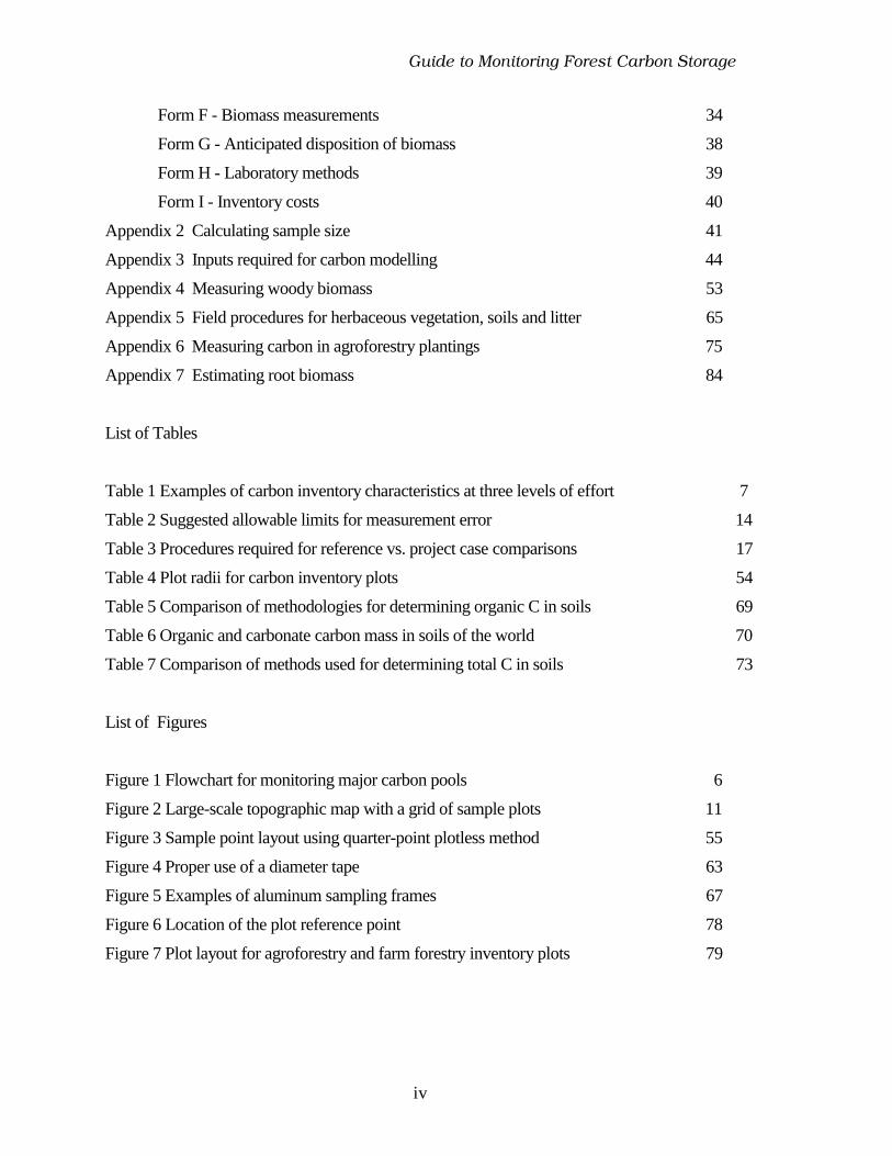
List of Tables
Table 1 Examples of carbon inventory characteristics at three levels of effort 7
Table 2 Suggested allowable limits for measurement error 14
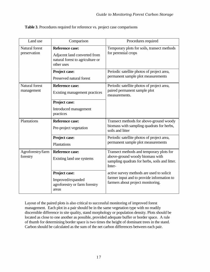
Table 3 Procedures required for reference vs. project case comparisons 17
Table 4 Plot radii for carbon inventory plots 54
Table 5 Comparison of methodologies for determining organic C in soils 69
Table 6 Organic and carbonate carbon mass in soils of the world 70
Table 7 Comparison of methods used for determining total C in soils 73
List of Figures
Figure 1 Flowchart for monitoring major carbon pools 6
Figure 2 Large-scale topographic map with a grid of sample plots 11
Figure 3 Sample point layout using quarter-point plotless method 55
Figure 4 Proper use of a diameter tape 63
Figure 5 Examples of aluminum sampling frames 67
Figure 6 Location of the plot reference point 78
Figure 7 Plot layout for agroforestry and farm forestry inventory plots 79

+YMHI�XS�1SRMXSVMRK�*SVIWX�'EVFSR�7XSVEKI
v
Acknowledgments
This guide is the product of the work of many individuals, and so there are many to thank.Financial support was provided by the Center for Environment, U.S. Agency for InternationalDevelopment and the Winrock International Institute for Agricultural Development. Versionsof this guide were reviewed for technical content by the following specialists:
Greg Biging, Dept. of Forestry, University of California at Berkeley, USA
C.B. Briscoe, Silviculturist, Turrialba, Costa Rica
H.E. Burkhart, Dept. of Forestry and Wildlife Resources, VPI, Blacksburg, VA, USA
David E. Chandler, Plantation specialist, Brasilia, Brazil
Noel Cutright, Senior Ecologist, Wisconsin Electric Power Company, USA
Paul Faeth, World Resources Institute, Washington, D.C., USA
Gina Green, The Nature Conservancy, Arlington, VA, USA
Tom Hanson, International Forestry Consultants, Inc., Bellevue, WA, USA
J.P. Kimmins, Dept. of Forest Science, University of British Columbia, Canada
H.G. Lund, U.S. Forest Service, Washington, D.C., USA
Vicente P.G. Moura, EMBRAPA, Vicosa, Brazil
Francisco de Paula Neto, Dept. of Forestry, Universidade Federal de Vicosa, Brazil
Michelle Pinard, University of Florida, Gainesville, Florida, USA
Maria das Gracas Ferreira Reis, Dept. of Forestry, Universidade Federal de Vicosa, Brazil
Jim Roshetko, Forestry/Natural Resources Management Program, Winrock International,USA
John Rombold, College of Forest Resources, University of Washington, USA
Roger Wilson, Programme for Belize, Belize City, Belize
Anthony Young, University of East Anglia, UK
Special thanks are due to Antonio Claret de Oliveira and Peter Althoff of the Mannesmann FI-EL Florestal Ltda. (Brazil), A. Joy Grant and Roger Wilson of the Programme for Belize,Geoffrey Blate and Johann Zweede of the Tropical Forest Foundation for their cooperationand support for field tests of these methods. Loren Ford, Ross Pomfrey and Mike Benge ofUSAID provided key administrative and technical support during the planning andimplementation stages. John Kadyszewski, Sinnammal Souppaya and Fay Ellis providedessential and much appreciated support through the Winrock Renewable Energy andEnvironment Program.
K.G. MacDicken, Senior Forestry Specialist
+YMHI�XS�1SRMXSVMRK�*SVIWX�'EVFSR�7XSVEKI
1
Summary
As the international Joint Implementation (JI) program develops a system for trading carboncredits to offset greenhouse gas emissions, project managers need a reliable basis formeasuring the carbon storage benefits of carbon offset projects.
Monitoring and verifying carbon storage can be expensive, depending on the level of scientificvalidity needed. This guide describes a system of cost-effective methods for monitoring andverification on a commercial basis, for three types of land use: forest plantations, managednatural forests and agroforestry. Winrock International’s Forest Carbon Monitoring Programdeveloped this system with its partners as a way to provide reliable results using acceptedprinciples and practices of forest inventory, soil science and ecological surveys. Perhaps mostimportant, the system brings field research methods to bear on commercial-scale inventories,at levels of precision specified by funding agencies.
Winrock’s system assesses changes in four main carbon pools: above-ground biomass, below-ground biomass, soils and standing litter crop. It aims to assess the net change in each pool forproject and non-project (or pre-project) areas over a specified time period.
Carbon monitoring efforts require specialized equipment, methods and trained personnel thatcan be expensive for individual organizations to procure and maintain. This is particularlytrue since most monitoring activities are likely to be performed infrequently — once everytwo to five years. In developing its monitoring system, Winrock has recognized these costsand aimed to minimize them. The system is therefore designed for collaboration between anorganization with specially-trained personnel and local organizations at each project site.
The system involves the following components:
• baseline determination of pre-project carbon pools in biomass, soils and standing littercrop
• establishment of permanent sample plots for periodic measurement of changes incarbon pools
• plotless vegetation survey methods (quarter point and quadrat sampling)1 to measurecarbon stored in non-project areas or areas with sparse vegetation
• calculation of the net difference in carbon accumulated in project and non-project landuses
1In woody savannah areas, the quarter point method helps in laying out measurement units by using thedistance between a systematic sampling point and the nearest tree or shrub. Quadrat sampling involves theuse of a portable sampling frame to delimit an area for measurement.

+YMHI�XS�1SRMXSVMRK�*SVIWX�'EVFSR�7XSVEKI
2
• use of SPOT satellite images as gauges of land-use changes, and as base maps for amicrocomputer-based geographic information system
• software for calculating minimum sample size, assigning sample unit locations (eitherin a systematic grid or randomly), determining the minimum spacing for plots andoptimizing site-specific monitoring plans
• computer modelling of changes in carbon storage for periods between fieldmeasurements
• a database of biomass partitioning (roots, wood and foliage) for selected species
A companion volume, entitled Field Tests of Carbon Monitoring Methods in ForestryProjects, will describe field experience with the methods contained in this guide.
+YMHI�XS�1SRMXSVMRK�*SVIWX�'EVFSR�7XSVEKI
3
1. Introduction
This guide describes methods and procedures for measuring the organic carbon stored byforestry and agroforestry land uses over time. Such a monitoring effort assesses the netdifference in organic carbon stored in soil2 and forest biomass for project and non-project (orpre-project) sites over a specified period of time. The difference in carbon stored is theamount of carbon sequestered, or ‘fixed’, by the project.
Carbon sequestration is thought to be a promising means for reducing atmospheric carbondioxide, an important greenhouse gas. To offset carbon emissions, at least 15 utilitycompanies and other organizations are involved in Joint Implementation (JI) land-use projectsinvolving plantations, improved forest management and natural forest preservation.3
A major constraint to successful forestry-based carbon offset programs is the lack of reliable,accurate and cost-effective methods for monitoring carbon storage. If carbon becomes aninternationally-traded commodity, as it appears likely, then monitoring the amount of carbonfixed by projects will become a critical component of any trading system. Current efforts atthe site level represent two extremes: either they are based on preliminary assumptions, orthey involve intensive research efforts that are too expensive for widespread use. The systemdescribed in this guide is intended to provide a cost-effective, precise and accurate accountingof carbon storage in projects. To the extent possible, the methods are standard approaches tomensuration and analysis of biomass and carbon.
Quantitative monitoring of carbon sequestration over time, and to a lesser extent verificationof estimates, requires a series of carbon inventories. For practical reasons, these inventoriesshould employ permanent sample plots, with periodic measurement of these sample plots inbaseline and project cases.4 Furthermore, the economic realities of the costs and benefits of acarbon inventory should be considered in the design stage, so that expectations of precisionare in harmony with the resources available for the monitoring effort.
1.1 Defining objectives
To maximize the utility of information collected in an inventory and to reduce monitoringcosts, forest managers should define the various objectives for an inventory early, in advanceplanning.
2 In general, these methods will be used to monitory only organic carbon. Inorganic carbon stored incarbonate materials is not likely to change with the vegetation changes anticipated in most forestry projects.3 Faeth, P., R. Livernash and C. Cort. 1993. Evaluating the carbon sequestration benefits of sustainableforestry projects in developing countries. Washington, DC: World Resources Institute.4 The baseline case is defined as on-site conditions without project activities. The project case includes on-site changes in soil and biomass carbon that occur due to project activities.

+YMHI�XS�1SRMXSVMRK�*SVIWX�'EVFSR�7XSVEKI
4
This guide assumes that the primary objective of carbon monitoring and verification is toproduce sound estimates of carbon sequestered by projects, for use in the trade of carboncredits (even though a system for trading carbon credits has not yet been finalized). Precisionis an important aspect of this objective. When an international carbon trading system isestablished, it will likely set precision standards for monitoring carbon in land-use systems.Until then, decisions on precision level must be made on a project basis as the monitoringobjectives are defined, so that the inventory can be designed to supply the desired precision.
It is possible and often desirable for a carbon inventory to have several concurrent objectives.The technical rigor required for carbon monitoring can drive the collection of other data onforest management, and make the process of forest monitoring more cost effective.Additional objectives might be to track important wildlife populations, or measure biologicaldiversity or timber species growth. The use of permanent sample plots also providesopportunities to study nutrient flows, production sustainability, and other trends.
1.2 Factors in inventory design
The use of permanent sample plots is generally regarded as a statistically superior means ofevaluating changes in forest conditions.5 Permanent plots allow efficient assessment ofchanges in carbon fixation over time, provided that the plots represent the larger area forwhich the estimates are intended. This means that the sample plots must be subject to thesame management as the rest of the project area. The use of permanent plots also allows theinventory to continue reliably over more than one rotation. Finally, permanent plots permitefficient verification at relatively low cost: a verifying organization can find and measurepermanent plots at random to verify, in quantitative terms, the design and implementation of aproject’s carbon monitoring plan. To achieve the same level of verification with temporarysample plots or other inventory approaches would require substantially more time andexpense.
The decision on which carbon pools to measure is critical to inventory design. In general, allpools that are large and subject to substantial change over the project life should be measured.Those that are small or very slow to change may not need to be measured. It is likely that aninternational carbon trading regime will require the project monitoring of all pools that arelikely to decrease over time.
For pools that are likely to increase, a key factor in the design of an inventory is the cost ofmeasurement and analysis of each component relative to the economic value of fixed carbon.For example, if carbon credits are worth US$2 per ton, it does not make economic sense tospend $2.50 per ton on measurements that include root biomass. However, it probably doesmake sense to spend $1.00 per ton on measurements that quantify roots.
In the current pilot phase of Joint Implementation (JI), it is assumed that carbon will haveeconomic value in the future.6 In terms of costs, most carbon sequestration projects have
5 For more details on this, see Forest Measurements, 3rd edition, eds. T.E. Avery and H.E. Burkhart (NewYork: McGraw-Hill, 1983) or Forest Mensuration, 3rd edition, eds. B. Husch, C.I. Miller and T.W. Beers(New York: John Wiley and Sons, 1982).6 Joint Implementation refers to cooperative development projects that seek to reduce or sequestergreenhouse gas emissions as described in the U.N. Framework Convention on Climate Change.

+YMHI�XS�1SRMXSVMRK�*SVIWX�'EVFSR�7XSVEKI
5
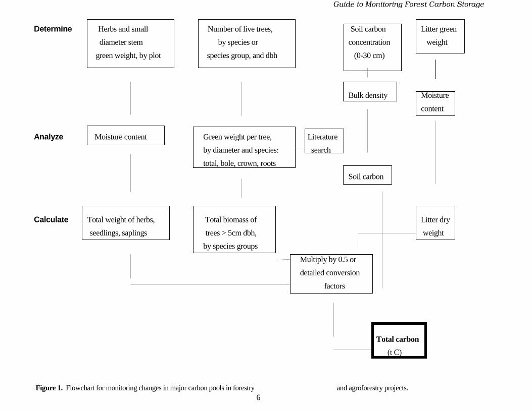
already calculated the cost of carbon fixed on a per ton basis. Inventories that follow thesystem described in this guide should be designed based on calculations of the cost per ton ofcarbon, as specified by the project implementor. Figure 1 outlines the overall process forinventory design and implementation.
1.3 Effects of product end useThe long-term effectiveness of carbon sequestration depends in part on the end-uses of thewood produced through project activities. The more durable the wood product, the greater theproject’s carbon storage effect in the medium and long term. However, carbon stored in woodis obviously not stored permanently; organic compounds eventually decay and some willultimately reappear as greenhouse gases. The impacts of carbon sinks are directlyproportional to the “ton-years” of storage (that is, tons of carbon multiplied by the number ofyears for which the carbon is stored). The methods described in this guide do not cover thestorage of carbon in post-harvest sinks. Anticipated disposition of biomass can be recorded inForm G.
Questions of “leakage”7 and off-site baseline changes are also important to the overall JointImplementation process. Off-site leakage may determine the success or failure of forestpreservation projects, but it is extremely difficult to quantify. Such off-site impacts areperhaps best estimated using the Land Use and Carbon Sequestration (LUCS) model availablefrom the World Resources Institute.8
7 In this context, leakage is the loss of carbon (primarily woody biomass) in non-project areas due toproject activities. For example, leakage occurs if a natural forest area that was previously used locally fortimber and firewood, is closed due to a preservation project, causing fuelwood and timber to be harvestedelsewhere.
8 For information on LUCS, contact the World Resources Institute, 1709 New York Ave., NW,Washington, DC 20006, USA.
+YMHI�XS�1SRMXSVMRK�*SVIWX�'EVFSR�7XSVEKI
6
Determine Herbs and small Number of live trees, Soil carbon Litter green
diameter stem by species or concentration weight
green weight, by plot species group, and dbh (0-30 cm)
Bulk density Moisture
content
Analyze Moisture content Green weight per tree, Literature
by diameter and species: search
total, bole, crown, roots
Soil carbon
Calculate Total weight of herbs, Total biomass of Litter dry
seedlings, saplings trees > 5cm dbh, weight
by species groups
Multiply by 0.5 or
detailed conversion
factors
Total carbon
(t C)
Figure 1. Flowchart for monitoring changes in major carbon pools in forestry and agroforestry projects.
+YMHI�XS�1SRMXSVMRK�*SVIWX�'EVFSR�7XSVEKI
7
Table 1. Examples of three levels of effort for carbon inventory
Level of effort General description
Basic This provides a very general, low-cost estimate of carbon stored inplantations. Less intensive sampling keeps costs low, but provides estimatesof mean carbon fixation with accuracy approaching 30% of the estimatedmean. Permanent sample plots are measured only twice: at plotestablishment and at final harvest. Modelling produces interim estimates ofcarbon fixation in vegetation and soils.
Moderate This level provides carbon storage estimates that are generally within 20%of the mean. Sampling intensity is greater, resulting in substantially moreprecise estimates than the basic inventory. Permanent plots are monitoredevery 2-3 years and at final harvest. Predictive models can be used toprovide estimates of annual carbon fixation but would not be used in mostapplications.
High This option produces estimates that are accurate within 10-15% of theamount of carbon sequestered, due to increased sampling and reducedreliance on models. Permanent sample plots are measured on an annualbasis.
1.4 Inventory outputsCarbon inventories of land-use projects can provide two general types of information: 1)carbon inventory reports that document changes in the quantities of carbon fixed due toproject activities, and 2) commercial timber inventories that document quantities ofmerchantable timber. This guide describes only the first type, i.e., reports that indicatechanges in carbon that result from project activities. Inventories of commercial timber,requiring slightly different data collection methods and analysis, can be done at relatively littleadditional cost.9
The inventory process usually yields two general types of outputs: baseline reports thatdescribe carbon pool sizes at the beginning of the project and periodic reports that describechanges in these pools based on repeated measurement. The initial baseline carbon reportprovides an estimate of the quantity and distribution of carbon in vegetation and soils. Thisbaseline would be produced before project activities begin and would serve as the benchmarkfrom which future changes in carbon pool size would be calculated. The baseline reportwould be produced only once per site.
9 For timber inventory methods compatible with those described in this guide, see Forest Measurements,3rd edition, eds. T.E. Avery and H.E. Burkhart (New York: McGraw-Hill, 1983) or Forest Mensuration,3rd edition, eds. B. Husch, C.I. Miller and T.W. Beers (New York: John Wiley and Sons, 1982).

+YMHI�XS�1SRMXSVMRK�*SVIWX�'EVFSR�7XSVEKI
8
Periodic inventory reports based on recurring measurement of permanent sample plots providethe basis for determining changes in carbon pools. These reports will describe measuredquantities and distribution of organic carbon pools in soils and vegetation in project and non-project lands and calculate the net carbon stored by project activities and will verify projectarea and changes in biomass and soil carbon.10 In order to measure carbon change due toproject activities, both the project and non-project cases must be monitored over time.
The methods in this guide have been field-tested under various conditions in Belize (OrangeWalk District), Brazil (Minas Gerais and Para), Guatemala (La Union), the Philippines(Isabela Province), and the United States (Washington and Oregon). The experiences of thesefield tests are recorded in a companion volume entitled Field Tests of Methods for MonitoringCarbon in Forestry Projects.
2. Measuring Carbon PoolsCarbon inventories are in effect “snapshots” of carbon stored at the time of the inventory. Toensure these snapshots can be usefully compared with each other, it is important for theinventory team to be consistent in its use of measurement techniques and methods betweendifferent sites, stands, and inventory periods.
The following four carbon pools can be inventoried using the methods outlined in this guide:
1. Above-ground biomass/necromass2. Below-ground biomass (tree roots)3. Soil carbon4. Standing litter crop
Appendices 4 - 6 describe the methods for measuring each of these carbon pools.
As mentioned earlier, permanent sample plots have two main advantages for carbonmonitoring: (1) they provide more reliable data on trends in vegetation development thantemporary plots do; and (2) they are more easily verified than other methods, since permanentplots can be revisited and remeasured by an external verifier.
The remainder of this guide refers to methods and procedures to be used with permanentsample plots that will be periodically monitored.
2.1 Inventory designFor the carbon inventories described in this guide, the sample unit is the permanent sampleplot. The sample frame (i.e., the listing of all the sample units) is the project’s land area,excluding buffer zones and areas that are not carbon sinks for project purposes.
10 While the largest largest proportion of carbon changes usually occur in biomass, soil carbon is alsolikely to change due to cultivation and conversion to new species. For a more detailed description of theeffects of land-use changes on soil carbon in the tropics, see Dynamics of soil organic matter in tropicalecosystems, eds. D.C. Coleman, J.M. Oades and G. Uehara (Honolulu: University of Hawaii Press, 1989).
+YMHI�XS�1SRMXSVMRK�*SVIWX�'EVFSR�7XSVEKI
9
Sampling design
There are four options for sampling design: complete enumeration, simple random sampling,systematic sampling and stratified random sampling. For carbon inventory, stratified randomsampling generally yields more precise estimates for a fixed cost than the other options.Stratified random sampling requires stratification, or dividing the populations into non-overlapping subpopulations. Each stratum (or subpopulation) can be defined by vegetationtype, soil type, or topography. For carbon inventory, strata may be most logically defined byestimated total carbon pool weight. Since that largely depends on above-ground biomass,stratification criteria that reflect biomass are generally most appropriate.
Useful tools for defining strata include satellite images, aerial photographs, and maps ofvegetation, soils or topography. These should be combined with ground measurements forverifying remotely-sensed images (or ground truthing). The key to useful stratification is toensure that measurements are more alike within each stratum than in the sample frame as awhole. A geographic information system (GIS) can automatically determine stratum size andthe size of exclusions or buffer zones (e.g., village sites, non-project areas within the largerproject area, stream buffers, archeological sites). Areas can also be determined manuallyusing a planimeter or dot grid.
Sample size
The level of precision11 required for a carbon inventory has a direct effect on inventory costsand, as noted earlier, needs to be carefully chosen by those who will use the inventory report.Once the level of precision has been decided upon, sample sizes must be determined for eachstratum in the project area and for each carbon pool to be measured. Carbon inventory is morecomplicated than traditional forest inventory in that each carbon pool may have a differentvariance (amount of variation around the mean). So, while the standard error of the mean forabove-ground biomass may be 20% of the mean, if the same sample sizes are used for eachcarbon pool the standard error for soil carbon may be 40%, and that for root biomass may be80% or more. To simplify sampling design and the understanding of the precision presentedin an inventory, sample sizes for each carbon pool should be determined separately. Afterthat, the inventory manager can decide how many samples to collect for each pool.
Appendix 2 describes a spreadsheet for inventory decisions that will calculate sample sizeusing standard formulae based on measured variation for the carbon pool to be sampled. Theappendix describes two alternatives for determining sample size and allocating sample plotsamong strata: 1) sample plot allocation based on fixed precision levels and, 2) optimumallocation of plots among strata given fixed inventory costs.
Permanent plots cannot always be relocated (or reoccupied) for a variety of reasons (e.g., plotmarkers are overgrown or are removed by people, plots are burned or records are lost). Tohelp ensure a minimum number of plots are available for remeasurement, it is prudent toincrease the number of plots above the minimum in the initial sampling design. Increasing theminimum number of plots for the baseline by 10-20% provides a “cushion” that helps to
11Precision is the degree of agreement in a series of measurements. Accuracy is the closeness of ameasurement to a true value.
+YMHI�XS�1SRMXSVMRK�*SVIWX�'EVFSR�7XSVEKI
10
ensure that the minimum precision requirements will be met even if there are missing plots insubsequent inventories.
If biomass or soil carbon data are not available for a site, preliminary samples should be takenfrom 10 plots of equal area, perhaps as a training exercise for technicians. These data shouldbe used to estimate the variance for calculating sample size.
Selection of sample units
The sample units will almost always be fixed-area permanent plots. Permanent plot locationscan be selected either randomly or systematically. If stratified random sampling is used,sample units for each stratum can still be selected systematically. If little is known about thepopulation being sampled, random selection of sample units is generally safer than systematicselection. If plot values are distributed irregularly in a random pattern, then both approachesare about equally precise. If some parts of the strata have higher carbon content than others,systematic selection will usually result in greater precision than random selection.
Map preparation
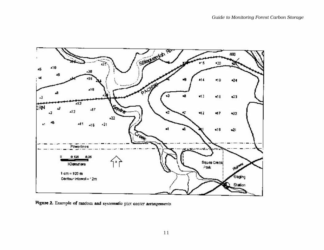
Once the sampling design, sampling sizes, and method for selecting sample units have beendetermined, the locations of the permanent sample plots must be marked on a map and/or thesatellite image. Accurate, well-annotated maps are essential for finding permanent sampleplots in the field. Using a GIS or desktop mapping system such as MapInfo can help automatethis process and reduce the possibility for error. In the topographic map in Figure 2, 25permanent sample plot locations in the eastern half of the map were determined using asystematic grid; sample units in the western half were selected randomly. Utilities for plotlocation allow precise descriptions of plot center locations and help crews to readily find anygiven plot with the use of a DGPS receiver.
A major advantage of mapping or GIS software is the ability to produce maps at manydifferent scales quickly, and therefore customize the scale for each set of users. For example,funding agencies may be interested in small-scale maps (e.g., 1:50,000) that provide anoverview of the project site. Project managers, on the other hand, may find larger-scale maps(1:25,000) more useful for viewing details of the project site that help them plan and manageall project components together. Field crews will generally want the largest-scale maps(1:10,000) to help them navigate. With a well-designed system for collecting and enteringdata, mapping software can automate most of this process.
A software package such as MapInfo, together with digital SPOT satellite images, can help aninventory manager to establish a systematic grid of sample plots at regular spacings andproduce a list of coordinates for each plot. If desired, the program can list distances andcompass bearings for navigating from plot to plot. However, these would normally beincluded in a route entered into the GPS receiver before the field crew begins each day’s tripto find and measure plots.
+YMHI�XS�1SRMXSVMRK�*SVIWX�'EVFSR�7XSVEKI
11

+YMHI�XS�1SRMXSVMRK�*SVIWX�'EVFSR�7XSVEKI
12
2.2 Inventory timingCarbon inventories are likely to be infrequent. Unless they involve continuous monitoring(and substantially greater expense), inventories cannot account for seasonal fluctuations in thesize of carbon pools. Because inventories measure carbon at just one point in the seasonalcycle, it is crucial to consider the seasonal timing of the inventory carefully before any otherplanning. In most cases, the inventory should take place during the season when field crewscan work most efficiently and safely. This will usually be the part of the dry season with themost favorable temperatures for strenuous field work. For smaller projects or those thatrequire fewer sample plots, selection of the season for inventory fieldwork can be moreflexible, since they will require less time in the field than larger projects.
To eliminate seasonality as a source of variation in inventory results, subsequent inventoriesmust be scheduled for the same season as the first inventory, preferably in the same month.
2.3 Measurement proceduresPermanent sample plots should be remeasured at an interval determined jointly by theinventory sponsor and manager, based on the desired level of precision. The only exception tothe use of permanent sample plots might be the case of a low-intensity inventory employing asingle assessment of biomass at the end of the tree-crop rotation. In this case, a conventionalinventory using either fixed plots, strips or 3P sampling12 can be used in place of permanentinventory plots.
If managers periodically inventory biomass (or wood volume) for commercial purposes, asecond alternative to measuring permanent plots may be available. In this case, data collectionfor non-timber carbon (e.g., litter, soil carbon, understory vegetation) could be added to thetimber inventory procedures during cruises in the project area.
Locating plots in the field
Two options exist for establishing and marking plot locations on the map and in the field:
Preferred option: Global Positioning System (GPS)
The use of GPS receivers to mark plot locations enables efficient and accurate placement andreoccupation of plots, particularly in projects with few roads. For natural forest projects orprojects in dense vegetation, sample plot locations should be established using differentialcorrection (to correct for systematic errors that result from the Defense Department’s practiceof “selective availability”).13 Differential correction ensures that plot centers are located asaccurately as possible. Initial plot location can be done using post-processing differentialcorrection with receivers capable of accuracy within 5 m. For crews to revisit plots in densevegetation, the project will require real-time differential correction capacity (i.e., either carrierphase DGPS to correct signals transmitted over radio waves, the use of differential beacons, asatellite correction system such as Omnistar or the use of radio-modems for both base stationand field crews).
12 3P sampling is sampling with probability proportional to prediction.13 A recent decision by the U.S. Government to remove selective availability will at some future timeobviate the need for differential correction for many forestry applications.

+YMHI�XS�1SRMXSVMRK�*SVIWX�'EVFSR�7XSVEKI
13
Alternative: Compass bearing and distance
Relative bearings can be taken from known landmarks for approach lines, distances andreference points for each plot. GPS coordinates can also be used as the basis for compassbearing and distance. This is particularly useful when steep topography or very dense canopycover at the plot site prevent reliable GPS readings. This information should be recorded onthe CIDF (Appendix 1, Form E).
Above-ground biomass in project plots
Measure above-ground project biomass using a timber cruise of permanent inventory plotsand biomass tables (Appendix 4). Measure the diameter of all woody vegetation of aminimum diameter and greater (e.g., > 2 cm) in dbh (diameter at breast height, 1.3 m). Paint amark on each stem at dbh to ensure correct measurement for the next inventory. Takesubsamples of smaller diameter woody vegetation and herbaceous plants using small quadratsor circular plots. Convert individual dbh values for each plot to biomass using single-entrybiomass tables. Where single-entry tables do not provide adequate estimates of biomass, usedouble-entry tables based on dbh and height (i.e., length). Appendix 6 describes how toestimate below-ground biomass.
For tree species for which biomass tables do not exist, the project may need to develop thebiomass tables. It is generally preferable to use biomass tables directly rather than to usewood-density values to convert stem wood volume tables to biomass, because wood densityvaries significantly among trees within a species. Biomass tables can be constructed using aminimum of 30 well-selected trees or with a “mean tree” approach (Appendix 4). Appendix 5describes methods for herbaceous vegetation.
A last alternative to developing biomass tables is to use the general biomass equations foundin Appendix 4. However, this alternative is not generally recommended due to the highvariability between species.
Above-ground vegetation on non-project sites
Quantifying changes in non-project (reference case) vegetation is, in most cases, essential forquantifying a project’s net carbon accumulation. Non-project vegetation will most likelychange
during the project period, so the only way to quantify project benefits reliably is to monitorvegetation on both project and non-project sites and calculate the difference in carbon stored.
Most non-project (reference case) areas will not be in heavy forest cover and may not requirepermanent sample plots. For example, in savannahs that are regularly burned or agriculturallands subject to tillage, plotless sampling methods can yield acceptable levels of precision atlower cost. The plotless quarter point method is described in Appendix 4.
Below-ground biomass
Even at moderate levels of precision, measuring root biomass is time consuming andexpensive due to the wide variability in the way that roots are distributed in the soil. For manyprojects, it might be best to estimate root biomass using a conservative ratio for shoot:root

+YMHI�XS�1SRMXSVMRK�*SVIWX�'EVFSR�7XSVEKI
14
biomass as the basis for claiming carbon credit. For example, the lowest shoot:root ratio everreported for Species X is 5:1. To develop a conservative estimate without measuring roots, aninventory could calculate root biomass as not less than 10 or 15% of above-ground biomass.
However, for cases in which more accurate estimates of below-ground biomass areeconomically feasible, Appendix 6 describes measurements using pit, auger/core sample andpinboard monolith methods.
Soils
Soils are often large storage pools for carbon, both organic and inorganic. Soil carbon can bedetermined effectively using composite samples that represent multiple plots. This helps toreduce costs of data collection and analysis, yet provides a reasonable estimate of soilproperties.14 The sample size calculator described in Appendix 2 can also be used tocalculate the number of samples required per composite soil sample. Appendix 5 describesmethods for sampling and measuring soil carbon.
Measurement standards and check cruising
Measurement standards define the maximum allowable error in measurements. Table 2provides suggested allowable limits of error. Measurements with error that exceed thesestandards should be rejected as unacceptable.
Table 2. Suggested allowable limits for measurement error
________________________________________________________________________
Measurement Allowable error
________________________________________________________________________
Tie lines
Bearing ±2o of the true bearing
Distance ±2o of the true horizontal distance
Permanent plots
Missed or extra trees No error within the plot
Tree species or groups No error
Breast height ± 5 cm of the true height (1.3 m)
D.B.H. ± 0.1 cm or 1% whichever is greater
Circular plot radius ±1% of horizontal
________________________________________________________________________
14 Peterson, R.G. and L.D. Calvin. 1982. Sampling. In Methods of soil analysis, part 1. AgronomyMonograph no. 9 (2nd Edition). ASA-SSSA, Madison, Wisconsin.

+YMHI�XS�1SRMXSVMRK�*SVIWX�'EVFSR�7XSVEKI
15
The following general standards are required for carbon inventories using permanent sampleplots:
1. Describe sample locations accurately enough to enable a crew to revisit the sampleplots.
2. Keep adequate records of all data.
3. Specify standards for stratification and sampling design for every inventory, andadhere to these standards carefully.
4. Take all measurements carefully, using properly adjusted instruments of provenaccuracy. Make every effort to eliminate personal bias by using well-understoodinstructions and factual observation in the field.
5. Calculate sampling errors.
6. Inadequate marking, measurement or recording of data, or the sloppy location ofplot centers, may indicate errors or biased location of sample plots. This may cause asponsoring agency to reject the inventory.
Check cruising is the verification of field measurements, and involves remeasuring apercentage of plots to ensure reliable, accurate data of known quality. Check cruising isnecessary for all cruise-based inventories. In general, check cruises should remeasure 1-5% ofall plots within two weeks after initial measurement. The crew performing remeasurementshould not include any members who participated in the initial measurements. Check cruisingshould be done with greater intensity (e.g., check cruising of 15% of the plots) for the firstweek’s plots. Measurements for the second week might be monitored using a check cruise of10%, and 5% for the third weeks’ plots. This provides crews with direct feedback on theirperformance and helps to correct procedural errors before they become expensive to correct.As confidence increases in the crews’ abilities to collect reliable data of known precision, thecheck cruise intensity might be reduced to random remeasurement of 1% of the plots.

+YMHI�XS�1SRMXSVMRK�*SVIWX�'EVFSR�7XSVEKI
16
3. Designing Monitoring Packagesfor Specific Land Uses
Project-specific monitoring must meet the specifications of the inventory sponsor and at thesame time use methods and procedures that are appropriate for the site. Different forest typesor land-uses may require different sets of the methods in this guide. Table 3 lists some of thecomparisons and procedures required for the kinds of land-use likely to be included in JointImplementation projects.
Packages of methods/procedures should be assembled to meet both the practical and technicalrequirements of a site (and the institution(s) conducting the monitoring and verification) andthe cost of using these methods. Section 3.1 discusses general aspects of monitoring design byland use. Sections 3.2 and 3.3 describe some of the important economic issues relevant tomonitoring designs for specific projects.
3.1 General requirements by land-use
Natural forest preservation
Natural forest preservation projects provide perhaps the greatest amount of fixed carbon in theearly years of a JI project because biomass density is high and deforestation at non-projectsites often releases large portions of stored carbon in biomass due to clearing, wood removalsand burning. The primary carbon comparisons required for these types of projects arebetween the areas being preserved and the land-use(s) the forest would be converted to if theforest were not protected.
Satellite images are important tools in the monitoring of preservation areas because theyprovide a clear record of land-use change. Permanent plots can provide reliable trend data oncarbon pool changes and are valuable in protected forest areas. If forest lands outside theprotected area are being converted to agricultural fields, the only measurements required in thereference case will be soil carbon. If the reference case lands contain woody biomass orgrasslands, then either permanent plots or transect methods are suggested for the measurementof biomass carbon.
Natural forest management
Monitoring the changes in carbon due to management of natural forests requires pairedcomparisons between forests managed with “improved” regimes and comparable areas usingreference case management. The differences in stored carbon are likely to be smaller innatural forest management projects than in forest preservation or plantations. This may meanthat for larger sample sizes will be required in forest management projects to attain the samelevel of precision as forest preservation or plantation projects.
+YMHI�XS�1SRMXSVMRK�*SVIWX�'EVFSR�7XSVEKI
17
Table 3. Procedures required for reference vs. project case comparisons
Land use Comparison Procedures required
Natural forestpreservation
Reference case:
Adjacent land converted fromnatural forest to agriculture orother uses
Temporary plots for soils, transect methodsfor perennial crops
Project case:
Preserved natural forest
Periodic satellite photos of project area,permanent sample plot measurements
Natural forestmanagement
Reference case:
Existing management practices
Periodic satellite photos of project area,paired permanent sample plotmeasurements.
Project case:
Introduced managementpractices
Plantations Reference case:
Pre-project vegetation
Transect methods for above-ground woodybiomass with sampling quadrats for herbs,soils and litter
Project case:
Plantations
Periodic satellite photos of project area,permanent sample plot measurements
Agroforestry/farmforestry
Reference case:
Existing land use systems
Transect methods and temporary plots forabove-ground woody biomass withsampling quadrats for herbs, soils and litter.Inter-
Project case:
Improved/expandedagroforestry or farm forestryareas
active survey methods are used to solicitfarmer input and to provide information tofarmers about project monitoring.
Layout of the paired plots is also critical to successful monitoring of improved forestmanagement. Each plot in a pair should be in the same vegetation type with no readilydiscernible difference in site quality, stand morphology or population density. Plots should belocated as close to one another as possible, provided adequate buffer or border space. A ruleof thumb for determining border space is two times the height of dominant trees in the stand.Carbon should be calculated as the sum of the net carbon differences between each pair.
+YMHI�XS�1SRMXSVMRK�*SVIWX�'EVFSR�7XSVEKI
18
Forest plantations
Plantations are often the easiest projects to monitor because when compared to natural foreststhey usually have higher road densities, better records and easier access to plots. Permanentplot methods are appropriate in forest plantations, although the easy access and greatermanagement intensity introduce a potentially high risk that the plots will be manageddifferently from surrounding project areas. To minimize that risk, plots should be markedinconspicuously using markers that are far from the actual plot centers coupled with a buriediron pipe or special marking magnets and a specialized metal detector. Plot locations shouldbe kept confidential to avoid the intentional application of additional inputs to the plots.
Satellite imagery provides a clear picture of plantation size and location. When analyzed withmapping software it also provides a ready means of calculating strata and total project areas.
Agroforestry and farm forestry
Spatial variability and farm to farm differences in management are the greatest challenges formonitoring agroforestry or farm forestry areas. Most projects of this type will include farmsthat are widely dispersed and managed in different ways. Many of the methods used tomeasure carbon sequestration in natural forests can be directly applied to agroforestryplantings, but there are some important differences. These include:
• agroforestry plantings require intensive labor inputs, and are typically small in size.
• agroforestry plantings are often widely scattered over the landscape. Broad expansesof non-project vegetation may separate individual plantings.
• trees in agroforestry plantations are often widely spaced to provide light for associatedcrops. As a result, the tree canopy is discontinuous and may be highly variable.
• in some agroforestry systems, trees are arranged in regularly spaced rows. This couldintroduce bias into systematic sampling schemes arranged in linear grid-like patterns.
• Agroforestry plantings are usually established and maintained by small landholders.Thus, any measurement of an agroforestry plantation necessarily involves professionalinteraction with farmers that may not occur in other types of land-use projects.
3.2 Setting economic limitsSome potential JI projects do not fix enough carbon for a monitoring effort to be economicallyworthwhile. Although this should be evaluated prior to project approval, it may be necessaryto make preliminary estimates of monitoring costs at the proposal development stage. Whendesigning a monitoring system, the cost of measuring each component should be estimatedand compared to the value of carbon. During the JI pilot phase there is no actual trading valuefor carbon, so the relative value of each measurement should be calculated and packaged in away that fits the project budget.
The monitoring package design should depend on how much carbon will be fixed per unitarea. For example, projects that fix less than 2 or 3 t C per hectare per year can not likely bemonitored in a cost-effective way because the costs of measuring these quantities are nearly

+YMHI�XS�1SRMXSVMRK�*SVIWX�'EVFSR�7XSVEKI
19
the same as the cost of monitoring 10 or 15 t C per hectare per year. When preparing amonitoring plan and budget, these economies of scale are important.
Project area is also an important factor in determining both the economic feasibility ofmonitoring and the cost per ton of carbon. In general, because fixed costs are a large part ofthe total monitoring cost, the larger the project area, the lower the unit costs for monitoring. Itis likely that projects smaller than 1,000 ha will be very difficult to monitor in a cost-effectiveway with reasonable precision.
+YMHI�XS�1SRMXSVMRK�*SVIWX�'EVFSR�7XSVEKI
20
4. ToolsBecause a carbon inventory might be estimating carbon worth millions of dollars, the tools forthese inventories need to be accurate, rugged and durable to withstand the rigors of field useunder adverse conditions. They should also contribute to efficient planning, data collection,analysis, and reporting. This section describes equipment for field work and software formodelling. Models can be useful tools for estimating changes in carbon pools for periodsbetween inventories; but for traded commodities, models are not adequate substitutes formeasurements.
4.1 Equipment In order to perform an inventory accurately, reliably and at minimum cost, an inventory teammust have good-quality equipment. Anything less can result in higher labor costs, greatersafety risks and unreliable carbon estimates. The following list of field tools and equipmentcontinues to evolve as methods are refined and new equipment becomes available. To someextent, equipment needs will vary with inventory objectives, available labor and skills, terrain,and vegetation or soil type. Figures 3 to 5 show examples of some of the equipment needed.
The following equipment and supplies are recommended for field crews:
Equipment
• compass/clinometer combination for navigation, plotting on the map, bearing andslope measurements
• diameter tape for measuring dbh
• loggers tape for measuring dbh and as a back-up for plot radius measurements
• Hagloff distance measure, tripod and extra threaded tripod adapter for measuringdistance to trees for diameters, and for measuring fixed plot boundaries
• calculator for calculating height, diameter
• cruisers vest for carrying cruising equipment
• entrenching tool, folding shovel or soil corer for taking soil samples
• precision spring scales (e.g., Pesola 1kg + 300g) + weighing bags, e.g., Tyvek 10 x17" bags (25.4 x 43.2 cm)
• sampling frames (2), round or square, hinged
• pruning saw and shears (e.g., Felco 60 and Felco 8)
• sheet holder
• two-way radio and extra batteries
• GPS (2) with differential correction capability and remote antenna mounted on fixedframe backpack (one as base station and one as remote), differential correctionsoftware, extra battery pack and charger
• notebook computer for database use and differential correction, and for generatingmaps

+YMHI�XS�1SRMXSVMRK�*SVIWX�'EVFSR�7XSVEKI
21
Supplies
• laminated maps or photos, with plot locations and coordinates
• pencils, marking pens, map scales
• ribbon (flagging) and painted high-grade PVC pipe for marking plot centers that areconspicuously marked
• plot cards, field aids and instructions
• rain gear
• safety equipment such as a first aid kit, hard hat, space blanket, waterproof matches,candle, insect repellent
• flashlight
• 50 cm x 50 cm piece of 5-mm mesh screen and small plastic tarp for screening andmixing soil samples
• sampling bags for soil, vegetation and litter, e.g., Tyvek 5 x 7" bags (12.7 x 17.8 cm)
Additional equipment for non-destructive biomass table measurements:
• Spiegel relaskop - metric scale for measuring tree diameters, heights and slope
• Jacob staff or monopod and ball joint adapter for use with relaskop
• bark gauge
• compact binoculars for use with relaskop
Additional equipment for verification measurements:
• hand-held data collection or pen-based computer
Additional requirements for real-time DGPS use in permanent plot reoccupation:
• radio modem transceivers (2)
• GPS base station capable of transmission
4.2 Models for interpolationThe size of carbon pools can be estimated for periods between inventories by using predictionmodels. Changes in soil and biomass carbon can be modeled using software packages such asSoil Changes Under Agroforestry (SCUAF), CENTURY and LUCS, using baseline surveydata and estimates of biomass growth. SCUAF Version 2.0 is recommended for use with themethods described in this guide, mainly for the following reasons:
• Ease of use. SCUAF is menu-driven and relatively user-friendly.
• Relevance. SCUAF was designed for use in agroforestry and incorporatesboth soil and biomass predictions for carbon and nitrogen.
• Presence of a default data set (for basic-level monitoring). Data on a numberof variables that are expensive to collect (e.g., root biomass, feedback factors,erosion rates) are provided in a default data set that has been carefully selectedfrom the literature.
+YMHI�XS�1SRMXSVMRK�*SVIWX�'EVFSR�7XSVEKI
22
• Cost and availability. SCUAF costs less than US$50 and is readily availablefrom the International Centre for Research in Agroforestry.15
• Documentation. The SCUAF manual is well written and provides goodinformation on the software’s theoretical basis and operations.
Appendix 3 describes the data collection requirements for SCUAF.
The prospect of saving on measuring costs by using computer models to predict future carbonstorage may be tempting. However, the costs of accurate, verified modelling are likely to be atleast as high as the costs of actual measurement, and perhaps greater. Modelling should onlybe used for interpolation, i.e., when investors require an estimate of carbon storage at a pointin time between two actual measurements.
15 International Centre for Research in Agroforestry, United Nations Avenue, Gigiri, P.O. Box 30677,Nairobi, Kenya.
+YMHI�XS�1SRMXSVMRK�*SVIWX�'EVFSR�7XSVEKI
23
5.0 Reporting and VerificationThe format and frequency of reports will depend in part on the inventory design, resources andthe reporting requirements of the sponsoring agency. Use the reporting formats described inthis section to present the results of carbon monitoring. Reports intended for use outside theproject’s technical staff should always include a summary explaining the consequences of thefindings.
5.1 ReportingThe way in which a project reports carbon credits will likely be determined by governmentalregulations or intergovernmental agreements. Until such guidelines are in place, the followingtwo types of reporting might be considered.
1. Report mean values for carbon stored along with confidence limits (at p=0.05). Theformula for confidence interval calcuations is:
CI = X ± tsX
where : t = a two-sided t value for a probability level of 0.05
sX
= the standard error of the mean from the carbon inventory
2. Report the Reliable Minimum Estimate (RME) as a conservative measure of theminimum quantity expected to be present with its probability.16 The formula for thiscalculation is:
RME = X − tsX
where : t = a one-sided t value for a probability level of 0.05 (i.e., use p=0.10in a two-tailed t table)
sX
= the standard error of the mean from the carbon inventory
For most current uses, reporting mean values with confidence intervals is probably mostappropriate given the need for maximum incentives to potential investors in carbon offsetprojects.
5.2 BaselineThis report provides an estimate of organic carbon as it is distributed invegetation and soils before start of the project. It is derived from data summarized in theCarbon Inventory Data Form (Appendix 1).
Project description
16 For more details see Dawkins, H.C. 1957. Some results of stratified random sampling of tropical highforest. Seventh British Commonwealth Forestry Conf. Item 7 (iii).

+YMHI�XS�1SRMXSVMRK�*SVIWX�'EVFSR�7XSVEKI
24
Site name:Contact person:Project sponsor(s):Project manager:Local name of project site:Address, State, Country:Latitude:Longitude:Elevation (m):Project species:
Accuracy level specifications
Baseline carbon distribution
Carbon pool
Area(ha)
Mean carbondensity
(Mg ha-1)Total carbon
(Mg)Confidence
interval (Mg)
Reference case Above-ground Below-ground Forest floor Soil to depth of 30 cmTotal - reference case
NA
Project case Above-ground Below-ground Forest floor Soil to depth of 30 cmTotal - project case
ha
NET CARBON STOREDTHROUGH PROJECTACTIVITY
5.3 Reporting carbon changes
This format is for use in reporting changes in carbon stored due to project activities.
Dates:Date of previous measurement:Primary person responsible for monitoring:
+YMHI�XS�1SRMXSVMRK�*SVIWX�'EVFSR�7XSVEKI
25
Description
Site name:Contact person:Sponsors:Project manager:Local name of site:Address, State, Country:Latitude:Longitude:Elevation (m):Primary species:
Accuracy level specifications
Site history since carbon statement or last inventory
Describe any significant changes in management, pest and disease problems, harvesting orother mortality.

+YMHI�XS�1SRMXSVMRK�*SVIWX�'EVFSR�7XSVEKI
26
Carbon distribution17
Carbon pool Area
(ha)
Mean carbondensity
(Mg ha-1)Total carbon
(Mg)Confidence interval
(Mg)
Reference case Above-ground Below-ground Forest floor Soil to depth of 30 cmTotal - reference case
NA
Project case Above-ground Below-ground Forest floor Soil to depth of 30 cmTotal - project case
ha
NET CARBON STOREDTHROUGH PROJECTACTIVITY
5.4 Verifying carbon monitoring estimatesVerification of carbon offset projects by a third party is similar to an accounting auditperformed by an objective party. For greatest efficiency and the most useful results, theregular monitoring team and the auditing organization should agree on procedures andmethods before start of the project.
A verification audit of carbon monitoring is a form of quality assurance that is presentlyrequired by the U.S. Initiative on Joint Implementation (USIJI). It is also likely to be requiredin future carbon offset land-use programs. Just as periodic audits are required for companiesinvolved in other types of trade, a system of verification will be necessary in order to avoidneedless litigation over project benefits and credits.
Agencies aiming to verify a forestry project’s carbon storage estimates might follow thegeneral procedures used by auditing firms in accounting. These include:
1. Prior agreement on carbon monitoring methods at the outset. If the verifying agency andthe project’s carbon monitoring team agree on a system of methods for measuring carbonbefore the project begins, then the process can be evaluated efficiently, with little danger ofproblems that would call monitoring estimates into question.
17Carbon estimates are based on samples taken from permanent, fixed-area plots in sites prior to sitepreparation for establishment.

+YMHI�XS�1SRMXSVMRK�*SVIWX�'EVFSR�7XSVEKI
27
2. Review of all monitoring records, including field data collection sheets,spreadsheet/database files, computer model outputs, maps, remote-sensing data, plans,analyses, and reports.
3. Inspection and calibration of measurement and analytical tools used by the monitoringteam.
4. Reoccupation and measurement of a random sample of the permanent plots used in theinventory.
5. If satellite imagery was not used to calculate project area for previous inventories, obtainand process images to verify project area.
+YMHI�XS�1SRMXSVMRK�*SVIWX�'EVFSR�7XSVEKI
28
Appendix 1: Carbon Inventory Data Form (CIDF)
Form A - Level of precision specifications
This form is designed to record instructions from the inventory sponsor regarding the desiredlevels of precision. (NOTE: Each carbon pool will likely have a unique variance and willrequire a unique sampling intensity to achieve a constant overall level of precision. Forexample, root biomass is likely to be more variable than above-ground biomass; foliagebiomass is usually more variable than stemwood biomass.)
Form of decision from inventory sponsors:
____ General level of precision ____ Specific confidence limits (%)
____ Optimum precision for fixed-cost____ Cost based on precision
If a general level of precision is specified, record below the detailed specifications formodelling vs. field data collection, cost limits from sponsors, and overall desire for precision(e.g. basic, moderate, high):
Percentage of plots to be established in excess of the calculated minimumrequirement:______%
Other specifications requested by inventory sponsor(s):

+YMHI�XS�1SRMXSVMRK�*SVIWX�'EVFSR�7XSVEKI
29
Form B - Project site description
A complete site description provides enough information to identify and locate the site and toallow some explanation of performance. Most data required for this form should be availablefrom the project manager.
Site name:
Contact person:
Local name of site:
Address, State, Country:
Elevation range (m):
Ecological zone or general site type:
Most common slope class (flat or gentle = 0-5o; intermediate = 5-10o; steep = 11-45o; verysteep >45o):
Mean annual rainfall (mm):
Rainfall regime (summer, winter, bimodal, uniform):
Maximum length of dry season (months <50mm):
Mean annual temperature (oC):
Surface soil texture (sand, loam, clay):
Sub-soil texture (sand, loam, clay):
Soil depth to impermeable layer (<25 cm, 25-50 cm, 50-100 cm, or >100 cm):
Surface soil pH (A horizon):
Sub-soil pH (B horizon):
Map with at least 3 latitude/longitude points18:
18 Points identified from: _____ local maps _____ known survey points_____ differentially corrected GPS coordinates _____ uncorrected GPS coordinates

+YMHI�XS�1SRMXSVMRK�*SVIWX�'EVFSR�7XSVEKI
30
Form C - Sampling design
This form should be used in conjunction with the explanation for calculating sample size(Appendix 2).
Sampling design: Stratified systematic sampling with random start
Basis of stratification:
Source of variance estimates:
Variable used for estimate:
Number of samples used for estimate of sample plot requirements:
Acceptable error (% of treatment mean):
Stratumnumber19
Vegetation
type
Area (ha) Mean biomass
(t ha-1)
Coefficient ofvariation (%)
Number ofsample plotsrequired20
TOTAL
Append a map of the project area with sample plot locations marked and and coordinates foreach permanent sample plot location.
19 Coding system: First letter = component (i.e., A or B), Second letter = Treatment (i.e., P =project case; R = reference case), Number = stratum number from vegetation map
20 As calculated using the Winrock inventory sample size calculator

+YMHI�XS�1SRMXSVMRK�*SVIWX�'EVFSR�7XSVEKI
31
Form D - Satellite images
Satellite imagery, taken on an annual basis, can document the project area in an unbiasedmanner. Panchromatic SPOT imagery is recommended for this use due to the availability of
high spatial resolution (10 m) in a 7.5’ or 15’ view. (However, this is a rapidly changingtechnology with new products and services constantly emerging.21) SPOT offers theadditional advantages of (1) the ability to program the satellite cameras to cover a specific areaat a specific time and (2) the convenience of images that do not require correction fortopographic displacement in a commonly used map format.
Project managers, sponsors and field crews should receive copies of ortho-corrected,panchromatic prints. Digital image processing allows the input of geo-referenced images in aGIS such as MapInfo or ARC/Info.
Land area (including total area and mortality due to fire, clearing, insect and disease pests)should be determined annually from new satellite photos. In cases where cloud coverprecludes the use of satellite photos, specify plans for either aerial photography or ground-based verification of the area. When ordering satellite images, the following parameters aregenerally needed:
Parameters or qualifiers Value
Spectral mode
Maximum acceptable cloud cover
Scene date window
Site location
Angle range
Imagery must be ordered at least two weeks before the start of the desired viewing window.Images take approximately four weeks to process after viewing.
21If satellite images are desired for other uses, such as species identification or monitoring of stand health,options include the more expensive Landsat Thematic Mapper (30 m resolution reflected) and SPOTmultispectral images (20 m resolution). For more information, see Monitoring vegetation change usingsatellite data, by B.N. Rock, D.L. Skole and B.J. Choudhury, inVegetation dynamics and global change,eds. A.M. Solomon and H.H. Shugart (New York: Chapman and Hall, 1993).
+YMHI�XS�1SRMXSVMRK�*SVIWX�'EVFSR�7XSVEKI
32
Form E - Permanent plot locations
It is essential to mark clearly and record the locations of permanent sample plots to ensureefficient reoccupation of the plots for later measurements. Plot center markers painted withflorescent paint and large quantities of bright colored flagging are recommended for markingplot centers. The following form can be used to record planned and actual plot locations.
When using a GPS receiver, the actual position will usually differ from the planned positiondue to the Defense Department’s policy of selective availability (which introduces ditheredsatellite signals containing intentional errors) and/or difficult terrain at the planned location. Inany case, it is important to record the actual position, using either the best average fix from theGPS receiver (if differential correction is not used) or the corrected position after thepermanent plots are established and the corrections made.
Please note: this form must be accompanied by a map indicating permanent plot locations.

+YMHI�XS�1SRMXSVMRK�*SVIWX�'EVFSR�7XSVEKI
33
Plot Locations
Cruiser ________________ Date ___/___/___
Project ________________ Country________________
Plot location method (circle one): GPS Compass
Strata
Plot Plot
Landmarkor known
Bearingfrom
Planned position Actual position*
Elev.
No. No. size point landmark Latitude Longitude Latitude Longitude (m) Comments
*If different from planned

+YMHI�XS�1SRMXSVMRK�*SVIWX�'EVFSR�7XSVEKI
34
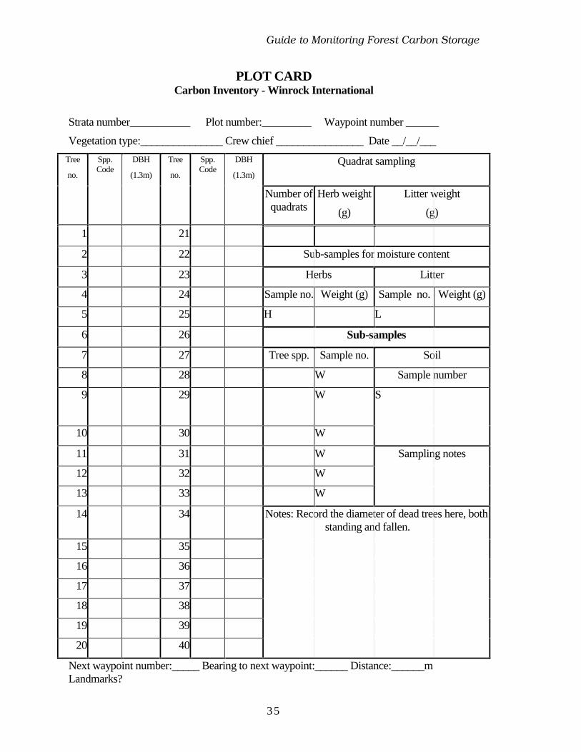
Form F - Biomass measurements
Biomass accumulation should be monitored periodically by measuring vegetation at projectand non-project sites. The plot card can be used to record measurements in permanent sampleplots. The quarter-point data collection sheet can be used for data collected using plotlessmethods.
+YMHI�XS�1SRMXSVMRK�*SVIWX�'EVFSR�7XSVEKI
35
PLOT CARDCarbon Inventory - Winrock International
Strata number___________ Plot number:_________ Waypoint number ______
Vegetation type:_______________ Crew chief ________________ Date __/__/___
Tree
no.
Spp.Code
DBH
(1.3m)
Tree
no.
Spp.Code
DBH
(1.3m)
Quadrat sampling
Number ofquadrats
Herb weight
(g)
Litter weight
(g)
1 21
2 22 Sub-samples for moisture content
3 23 Herbs Litter
4 24 Sample no. Weight (g) Sample no. Weight (g)
5 25 H L
6 26 Sub-samples
7 27 Tree spp. Sample no. Soil
8 28 W Sample number
9 29 W S
10 30 W
11 31 W Sampling notes
12 32 W
13 33 W
14 34 Notes: Record the diameter of dead trees here, bothstanding and fallen.
15 35
16 36
17 37
18 38
19 39
20 40
Next waypoint number:_____ Bearing to next waypoint:______ Distance:______mLandmarks?

+YMHI�XS�1SRMXSVMRK�*SVIWX�'EVFSR�7XSVEKI
36
Quarter Point Method Data Collection Form
Line number: Litter samples Vegetation
Point
number
Quarter
number
Species or
Speciesgroup code
DBH
(1.3m)
Diameter
@30cm
Height
(m)
Distance
(m)
Soilsample
NumberNumber
Sampleweight
Number
Sampleweight
1
2
3
4
1
2
3
4
1
2
3
4
1
2
3
4
1
2
3
4
1
2
3
4
1
2
3
4
1
2
3
4
1
2
3

+YMHI�XS�1SRMXSVMRK�*SVIWX�'EVFSR�7XSVEKI
37
Form G - Anticipated disposition of biomass
To gauge the effectiveness of carbon sequestration projects, it is essential to have an idea of theintended fate or end-use of the biomass grown.
Check one or more option. If more than one, then indicate approximate percentage of disposition foreach category.
____ Durable timber products (e.g., furniture, construction)
____ Pulp
____ Fuelwood (firewood or charcoal)
____ Foliage uses
____ Other (specify)
Non-project land use
____ Grazing
____ Periodic burning (specify approximate frequency)
____ Crops
____ Other (specify)

+YMHI�XS�1SRMXSVMRK�*SVIWX�'EVFSR�7XSVEKI
38
Form H - Laboratory methodsSoil and biomass carbon testing must be conducted by an established, reputable laboratory capable ofperiodic analyses throughout the project period. Total carbon is most often measured by either the drycombustion or wet combustion methods described by Nelson and Sommers.22 For soils that havecarbonate minerals present, corrections need to be made for inorganic carbon using one of themethods described by Nelson and Sommers. Total nitrogen will be analyzed using the regularKjeldahl distillation method, as described in Bremner and Mulvaney.23
Laboratory: ____________________________________
Address: _______________________________________
_______________________________________
_______________________________________
Telephone: ______________________ Fax number: __________________________
Contact person for analysis: ________________________________________
Carbon analysis methods (check one):
____ dry combustion in a resistance furnace
____ dry combustion in a induction furnace
____ dry combustion using automated methods
____ wet combustion using a combustion train
____ wet combustion using a Van Slyke-Neil apparatus
____ other (specify)
Cost per sample _____
Total nitrogen analysis methods (check one):
____ regular Kjeldahl distillation method
____ modified Kjeldahl distillation method (describe)
____ other (specify)
Cost per sample _____
Notes:
22 Nelson, D.W. and L.E. Sommers. 1982. Total carbon, organic carbon and organic matter. In Methods of soilanalysis, part 2. Agronomy Monograph no. 9 (2nd Edition). Madison, Wisconsin: ASA-SSSA.
23 Bremner, J.M. and C.S. Mulvaney. 1982. Nitrogen - total. In Methods of soil analysis, part 2. AgronomyMonograph no. 9 (2nd Edition). Madison, Wisconsin: ASA-SSSA.

+YMHI�XS�1SRMXSVMRK�*SVIWX�'EVFSR�7XSVEKI
39
Form I - Inventory costsThe amount of time and money required to collect and analyze baseline and annual carbon data shouldbe documented in this form. The most important use of this data will be for estimating the cost ofsampling in each stratum to determine the optimum allocation of sample plots.
Cost per Total
Man-day days Cost
Planning
SupervisionMaterialsTransportationOther
Training
InstructorsMaterialsOther
Quarter point method survey
SupervisionLaborTransportationOther
Permanent plot establishment
SupervisionLaborTransportationOther
Permanent plot monitoring
SupervisionLaborTransportationOther
Analysis, interpretation and reporting
PersonnelLaboratory analysesMaterialsOther
Total inventory costs

+YMHI�XS�1SRMXSVMRK�*SVIWX�'EVFSR�7XSVEKI
40
Appendix 2: Calculating Sample SizeThe spreadsheet that follows includes sample data from non-project stands as an example of how thecalculator can be used. Two approaches are used for determining sample size and sample plotallocations among strata: 1. optimum plot allocation based on fixed precision levels and, 2. optimumallocation of plots among strata given fixed inventory costs.24
1. Optimum plot allocation based on fixed precision levelsUse the following formula to calculate the number of sample units required to obtain a desiredstandard of precision:
n =t
A
2
WhSh Ch
h=1
L
∑
WhSh / Ch
h=1
L
∑
where n = sample size (i.e., total number of sample plots required)
t = tabular value of Student’s t
h = stratum number
L = the number of strata
Wh = Nh/N
Nh = number of sample units in stratum h
N = total number of sample units
S = stratum standard deviation
A = allowable error expressed in units of the mean
Ch = the cost of selecting a sample plot in stratum h
Allocation of these sample plots among strata is calculated as: nh = nph
where: nh = number of sample plots for stratum h
n = total number of sample plots
and
Ph = W hSh / C h( )/ W hSh / Chh =1
L
∑
24 For a more detailed description of this approach see Forestry handbook (2nd edition), ed. K.F. Wenger (NewYork: John Wiley and Sons, 1984) and Sampling techniques (3rd edition), by W.G. Cochran (New York: JohnWiley and Sons, 1977).
+YMHI�XS�1SRMXSVMRK�*SVIWX�'EVFSR�7XSVEKI
41
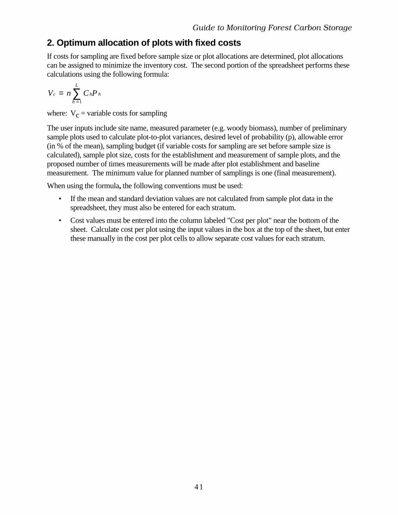
2. Optimum allocation of plots with fixed costsIf costs for sampling are fixed before sample size or plot allocations are determined, plot allocationscan be assigned to minimize the inventory cost. The second portion of the spreadsheet performs thesecalculations using the following formula:
Vc = n ChP h
h =1
L
∑where: Vc = variable costs for sampling
The user inputs include site name, measured parameter (e.g. woody biomass), number of preliminarysample plots used to calculate plot-to-plot variances, desired level of probability (p), allowable error(in % of the mean), sampling budget (if variable costs for sampling are set before sample size iscalculated), sample plot size, costs for the establishment and measurement of sample plots, and theproposed number of times measurements will be made after plot establishment and baselinemeasurement. The minimum value for planned number of samplings is one (final measurement).
When using the formula, the following conventions must be used:
• If the mean and standard deviation values are not calculated from sample plot data in thespreadsheet, they must also be entered for each stratum.
• Cost values must be entered into the column labeled "Cost per plot" near the bottom of thesheet. Calculate cost per plot using the input values in the box at the top of the sheet, but enterthese manually in the cost per plot cells to allow separate cost values for each stratum.

+YMHI�XS�1SRMXSVMRK�*SVIWX�'EVFSR�7XSVEKI
44

+YMHI�XS�1SRMXSVMRK�*SVIWX�'EVFSR�7XSVEKI
44
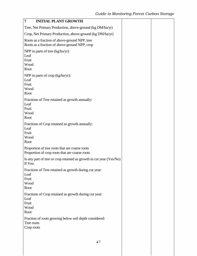
Appendix 3: Inputs for Carbon Modelling with SCUAF
The data required for carbon modelling using the Soil Changes Under Agroforestry (SCUAF)software are listed in the table below. Data on soil organic carbon, tree growth rates, biomasspartitioning, and site descriptions must be entered before running models. All inputs, includingdefaults, must be listed in the form. If data other than the default values are used, the source of thisdata should be listed in the "Source" column.
The following are inputs required to use SCUAF:25
Input Value Source
1 CYCLE
Cycle selected for modelling
If carbon cycle only is selected, it is not necessary to inputdata on nitrogen.
1 CarbonCycle
2 Carbonand NitrogenCycles
2 DOCUMENTATION
File nameTitleSourceLocationDateNotes
25The source references indicate values that are different from the SCUAF default data set.

+YMHI�XS�1SRMXSVMRK�*SVIWX�'EVFSR�7XSVEKI
45
3 PHYSICAL ENVIRONMENT
Climate:
Soil texture:
Drainage:
Soil reaction:
Slope class:
1 Lowlandhumid2 Lowlandsubhumid3 Lowlandsemi-arid4 Highlandhumid5 Highland subhumid6 Highlandsemi-arid
1 Mediumtextured2 Sandy3 Clayey
1 Free2 Imperfect3 Poor
1 Stronglyacid2 Acid3 Neutral4 Alkaline
1 Flat2 Gentle3 Moderate4 Steep
4 AGROFORESTRY SYSTEM
Length (years) Fraction of land under trees Fraction of land under crop Is it a cut year? (Yes/No) What fraction of tree is N-fixing? What fraction of crop is N-fixing?
Period
1 2 3 4 5 6

+YMHI�XS�1SRMXSVMRK�*SVIWX�'EVFSR�7XSVEKI
46
5 INITIAL SOIL CONDITIONS
DEPTH
Topsoil depth (cm) Soil depth considered (cm) Total depth of soil (cm)
CARBON
Initial Carbon, Topsoil (percent) Initial Carbon, Subsoil (percent) Bulk density, Topsoil (g/cc) Bulk density, Subsoil (g/cc) Initial soil Carbon (kg/ha)
NITROGEN
Initial Nitrogen, Topsoil (percent) Initial soil Nitrogen (kg/ha)
6 EROSION
Soil Erosion (kg/ha/yr) = Climate Factor * Soil Erodibility Factor* Slope Factor * Cover Factor * 1000
Enter best estimate for each factor:
Climate factorSoil erodibility factorSlope factorCover factor under treeCover factor under crop
Soil erosion under tree (kg/ha/yr)Soil erosion under crop (kg/ha/yr)
Tree proportionality factor
Measured soil erosion in Year 1 (kg/ha/yr)
Carbon enrichment factorNitrogen enrichment factor
+YMHI�XS�1SRMXSVMRK�*SVIWX�'EVFSR�7XSVEKI
47
7 INITIAL PLANT GROWTH
Tree, Net Primary Production, above-ground (kg DM/ha/yr)
Crop, Net Primary Production, above-ground (kg DM/ha/yr)
Roots as a fraction of above-ground NPP, treeRoots as a fraction of above-ground NPP, crop
NPP in parts of tree (kg/ha/yr):LeafFruitWoodRoot
NPP in parts of crop (kg/ha/yr):LeafFruitWoodRoot
Fractions of Tree retained as growth annually:LeafFruitWoodRoot
Fractions of Crop retained as growth annually:LeafFruitWoodRoot
Proportion of tree roots that are coarse rootsProportion of crop roots that are coarse roots
Is any part of tree or crop retained as growth in cut year (Yes/No)If Yes:
Fractions of Tree retained as growth during cut year:LeafFruitWoodRoot
Fractions of Crop retained as growth during cut year:LeafFruitWoodRoot
Fraction of roots growing below soil depth considered:Tree rootsCrop roots

+YMHI�XS�1SRMXSVMRK�*SVIWX�'EVFSR�7XSVEKI
48
CARBON
Carbon Fraction in dry mass, TreeCarbon Fraction in dry mass, Crop
NITROGEN
Nitrogen % in:orCarbon:Nitrogen ratio of:
Tree LeafTree FruitTree WoodTree RootCrop LeafCrop FruitCrop WoodTree Root or Crop Root
8 ADDITIONS
Organic (kg DM/ha/yr)
Carbon fraction in organic additionsNitrogen percent in organic additions or Carbon:Nitrogen ratio in organic additions
Fertilizer (kg/ha/yr)
Nitrogen fraction in fertilizer
Period
1 2 3 4 5 6
Period
1 2 3 4 5 6

+YMHI�XS�1SRMXSVMRK�*SVIWX�'EVFSR�7XSVEKI
49
9 REMOVALS
A: HARVEST
Fraction of Tree harvested annually:LeafFruitWoodRoot
Fraction of Crop harvested annually:LeafFruitWoodRoot
Additional fraction of Tree harvested in cut year:LeafFruitWoodRoot
Additional fraction of Crop harvested in cut year:LeafFruitWoodRoot
B: OTHER LOSSES FROM SYSTEM
Are there any losses of plant material from the systemother than harvest (e.g. burning)? (Yes/No) If Yes:
Fraction of Tree lost annually:LeafFruitWoodRoot
Fraction of Crop lost annually:LeafFruitWoodRoot
Additional fraction of Tree lost in cut year:LeafFruitWoodRoot
Additional fraction of Crop lost in cut year:LeafFruitWoodRoot

+YMHI�XS�1SRMXSVMRK�*SVIWX�'EVFSR�7XSVEKI
50
10 SOIL PROCESSES
CONVERSION LOSSES (Litter to Humus)
Fraction of above-ground parts lost through oxidation
Fraction of roots lost through oxidation
Fraction of organic additions lost through oxidation
Fraction of coarse tree roots decaying at least 1 year later
Fraction of coarse crop roots decaying at least 1 year later
Fraction of remaining coarse tree roots decaying 2 years later
Fraction of remaining coarse crop roots decaying 2 years later
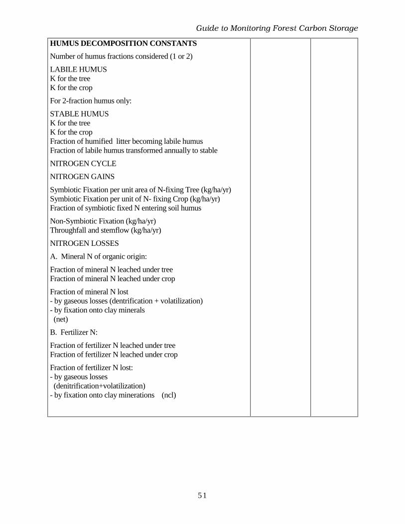
+YMHI�XS�1SRMXSVMRK�*SVIWX�'EVFSR�7XSVEKI
51
HUMUS DECOMPOSITION CONSTANTS
Number of humus fractions considered (1 or 2)
LABILE HUMUSK for the treeK for the crop
For 2-fraction humus only:
STABLE HUMUSK for the treeK for the cropFraction of humified litter becoming labile humusFraction of labile humus transformed annually to stable
NITROGEN CYCLE
NITROGEN GAINS
Symbiotic Fixation per unit area of N-fixing Tree (kg/ha/yr)Symbiotic Fixation per unit of N- fixing Crop (kg/ha/yr)Fraction of symbiotic fixed N entering soil humus
Non-Symbiotic Fixation (kg/ha/yr)Throughfall and stemflow (kg/ha/yr)
NITROGEN LOSSES
A. Mineral N of organic origin:
Fraction of mineral N leached under treeFraction of mineral N leached under crop
Fraction of mineral N lost- by gaseous losses (dentrification + volatilization)- by fixation onto clay minerals (net)
B. Fertilizer N:
Fraction of fertilizer N leached under treeFraction of fertilizer N leached under crop
Fraction of fertilizer N lost:- by gaseous losses (denitrification+volatilization)- by fixation onto clay minerations (ncl)

+YMHI�XS�1SRMXSVMRK�*SVIWX�'EVFSR�7XSVEKI
52
11 SOIL/PLANT FEEDBACK FACTORS
CARBON
Rise or fall in soil carbon, relative to initial state, of 1
percent causes increase or decrease in rate of plant growth by xpercent:
For Tree
For Crop
NITROGEN
Rise or fall in soil nitrogen, relative to initial state, of 1 percentcauses increase or decrease in rate of plant growth by x percent:
For Tree
For Crop
SOIL DEPTH
Rise or fall in soil depth, relative to initial state, of 1 percentcauses increase or decrease in rate of plant growth by x percent:
For Tree
For Crop
NOTES
+YMHI�XS�1SRMXSVMRK�*SVIWX�'EVFSR�7XSVEKI
53
Appendix 4: Measuring Woody BiomassWoody biomass will nearly always be the largest and most easily manipulated carbon pool in carbonstorage forestry projects. The inventory approaches for woody biomass are:
1. Measure the woody biomass of trees larger than a minimum diameter (e.g. >5 cm dbh) inproject and non-project areas using timber cruises of permanent, continuous inventory sampleplots. At the same time, sample the herbaceous biomass, standing litter crop and soil carbonvegetation, using the methods described in Appendix 5.
2. If permanent plots are not desirable or practical (due to frequent wildfire or grazing, forexample), use the plotless quarter point vegetation survey to evaluate biomass and carboncontent of vegetation on non-project sites. In plantation projects, the quarter-point method(which uses the distance between a systematic sampling point and the nearest tree or shrub)can be used to monitor lands left under natural vegetation. For preservation projects, thismethod can be used to monitor changes in lands converted to agriculture or other land useswith low tree population densities.
A. Timber cruisingUse permanent, inventory plots to measure timber on project and non-project sites, following astratified random sampling design. In general, most carbon sequestered by project activities will occurin the largest diameter classes, so the timber cruise part of the inventory requires particular care.
Size and shape of fixed plots
Circular plots established using a well-identified plot center and a digital distance measure arerecommended (Table 4). Optimal plot size can also be calculated using the following formula26:
Size = P1
t 2
m
where: P1= size of plot used in preliminary sample to assess time and variation in any unit of area; t =
average travel time between neighboring plots in minutes; m=average plot measurement time for plotsize P1 in minutes
To calculate optimal plot size, measure a minimum of three plots of size P1. Plots should be separatedby the same distances anticipated in an actual inventory. Travel speed between plots and the plotmeasurement time (m) should be recorded. Calculate t by dividing the distance between neighboringplots by the travel speed or measure and average travel time between plots. Calculate P using theformula above.
26 Zeide, B. 1980. Plot size optimization. Forest Science 26:251-257.

+YMHI�XS�1SRMXSVMRK�*SVIWX�'EVFSR�7XSVEKI
54
Table 4. Plot radii for carbon inventory plots
Plot size (m2) Plot radius (m) Area per tree (m2 tree-1) Application
100 5.64 0 - 15 Very dense vegetation, standswith large number of smalldiameter stems, uniformdistribution of larger stems
250 8.92 15 - 40 Moderately dense woodyvegetation
500 12.62 40 - 70 Moderately sparse woodyvegetation
666.7 14.56 70 - 100 Sparse woody vegetation
1,000
or use quarterpoint method
17.84 > 100 Very sparse woody vegetation
Relating diameter to biomass
Biomass tables or equations are needed to relate dbh and the number of plants per ha to total biomass.Biomass tables should therefore be sought for important species of native vegetation. Where thesetables are not available, there are three alternatives:
1. Develop biomass tables for each important tree species using the method described insection C of this appendix. This is the most precise (and most costly) approach.
2. Develop biomass tables for groups of tree or shrub species. The most useful groupings maybe by morphology class (e.g., single-stemmed trees, multiple-stemmed trees, shrubs).
3. Use one of the general biomass equations found in section C. This is the least preciseapproach, but also the least expensive. Given the wide range of species included in theseequations, they should not be used except where the alternatives above are not possible.
B. Non-project woody vegetationThis method should be used to measure natural vegetation prior to project establishment at the sameinterval set for the measurement of the permanent inventory plots in the project. To save time inlaying out plots in measuring woody savannah vegetation, use the quarter point method,27 whichuses the distance between a systematic sampling point and the nearest tree or shrub.
The steps for this method are:
1. Establish a series of parallel sample lines 100 m apart. Locate sample points every 10 malong each line.
27 For a more detailed description of this approach see Methods of sampling lesser vegetation, pp. 58-59 in Forestryhandbook (2nd edition), ed. K.F. Wenger (New York: John Wiley and Sons, 1984).

+YMHI�XS�1SRMXSVMRK�*SVIWX�'EVFSR�7XSVEKI
55
2. At each sample point, divide the immediate area into quarters using the sample line plus asecond line that crosses the sample point perpendicularly to the sample line. Figure 3demonstrates placement of line and sample point, along with quarter numbers for each samplepoint.
3. Collect species and diameter data using the data collection form. For shrubs and small treeswith low branching, measure diameter at 30 cm above the ground; for trees with better treeform, use dbh at 1.3 m. Also record the distance from each tree or shrub to the sample point.A minimum of 100 distance measurements are required per stratum.
4. Calculate average distances as follows:
• Average the four distances at each point, then average the distances for the entiresample area. Use this number to calculate the mean area per tree as: M = d2, where M= mean area per tree in m2 and d = average distance over the entire sample area.
• For the total sample area, calculate density using the formula: D = 10,000 / M,where D = trees per hectare.28
• Construct a stand table, with appropriate size diameter classes, and estimate biomassbased on a biomass table.
28 If only a few species predominate, then accuracy is probably increased by determining biomass and carboncontent by individual species. The method outlined in this section presumes relatively high species diversity andrelatively low return to the additional investment needed to estimate non-project biomass by species.

+YMHI�XS�1SRMXSVMRK�*SVIWX�'EVFSR�7XSVEKI
56
C. Developing biomass tables29Tree biomass weight tables show the average weight ofindividual trees for one or more dimensions, usually stem diameter alone (for local tables) or stemdiameter along with height or length. The tables employ data obtained in destructive sampling.Through regression analysis, wood or foliage weight can be related to dbh, diameter at 0.3 m, andheight. This appendix describes the process for developing standard biomass weight tables.Developing local weight tables is not recommended in view of their limited application and the greatdeal of effort they require, as well as the duplication of effort they involve.
Planning a weight table
Critical decisions must be made before beginning to develop a weight table, including:
• Defining the range of tree or shrub dimensions to be covered by the table.
• Defining the type(s) of biomass to be included in the table(s); this may include stem wood,stem and branch wood, or foliage; a table will need to be developed for each biomass type.
• Determining what measurements to use in relating biomass to a practical field measurement(e.g., d, dbh, or h).
• Defining size classes throughout the range of tree sizes.
Field sampling
A key issue is the number of trees necessary to develop a weight table for a given species. Estimatesfrom many recent biomass studies suggest that 30-100 trees are enough for a regional table usingstratified sampling of the population. Sufficient evidence supports the case that if sample trees areselected in equal or near-equal numbers for each size class, 30 trees for an individual tree biomasstable are adequate. At least 30 well-selected trees should be used per species for individual treebiomass tables, unless the tables are to be used only for a specific site. For such purposes, as few as12 trees may be adequate.
For calculating foliar nutrient content, more samples may be needed for foliage and branches than forstem wood. If scarce funds prevent the measurement of more than 30 sample trees for foliage,consider reducing the number of samples for stem wood in order to make resources available forfoliage and branch sampling.
Partitioning and weighing
Each individual tree or shrub should be harvested; measured for diameter, length, and height30; anddivided into the major components defined during the planning stage. Length measurements arerecommended, but if vertical height is to be included as an independent variable, the measurementmust be taken before the tree is harvested. Individual components (stem, branches, leaves, etc.)should be divided into several size classes for convenient handling and sub-sampling. Sub-samplesshould be taken to determine moisture content and specific gravity.
Techniques for weighing tree components depend largely on tree size and the availability ofequipment. Take care to keep each tree and its parts separate from other trees. The best way to ensure
29This section is taken largely from Standard research methods for multipurpose trees and shrubs, eds. K.G.MacDicken, G.V. Wolf and C.B. Briscoe (Arlington, Virginia: Winrock International, 1991).
30Length is the measured distance of a tree or specified portion of a tree following the lean or curvature, notnecessarily vertical or straight; height is the vertical distance between a standing tree’s apical bud and ground level.

+YMHI�XS�1SRMXSVMRK�*SVIWX�'EVFSR�7XSVEKI
57
this is to partition and weigh only one tree at a time. Measure green weight in the field. To calculatemoisture content, sub-samples should be taken, dried at 80Û�&�DQG�UH�ZHLJKHG�
Although harvesting is the preferred way to develop weight tables, it is not always possible due toconservation or regeneration considerations. For biomass tables from non-destructive samples,calculate stemwood volumes and convert them to biomass using specific gravity for wood andexpansion factors for canopy biomass. This requires a device for measuring diameter, such as aWheeler pentaprism caliper, Spiegel Relaskop or laser measuring device. A sample form forrecording data to construct biomass tables or volume tables using a metric Relaskop follows.
Analysis
Regression analysis should be performed for each biomass type defined during the planning process.To make the tables useful for the widest possible range of environments, at least one complete set ofequations and weight tables should include both diameter and height terms.

+YMHI�XS�1SRMXSVMRK�*SVIWX�'EVFSR�7XSVEKI
58
The most common equations for biomass types include:
____________________________________________________________________________
Biomass Type Most Common Equation(s)*
____________________________________________________________________________
Whole Tree B = b0 + b1D
2H
B = b0 + b1D
Woody Biomass B = b0 + b1D2H
Branch, Foliage, B = b0 + b1D2
or Crown Weight B = b0 + b1D
____________________________________________________________________________
*B = predicted total or above-ground biomass, D = diameter (cm) at breast height (1.3 m), H = totalheight (m), b0 and b1 = regression parameters estimated from the data.
Results should be represented as both regression equation and table to allow the widest possibleapplication of the work. When tables are unavailable and it is not practical to develop species-specificbiomass tables, the following general equations can be used:
Climate type based onannual rainfall
Equation R2 adjusted
Dry (<1500 mm) y = 34.4703 - 8.0671 D + 0.6589 D2 .67
Moist (1500-4000 mm) y = 38.4908 - 11.7883 D + 1.1926 D2
y = exp[-3.1141 + 0.9719 ln( D2H)]y = exp[-2.4090 + 0.9522 ln( D2HS)]
H = exp[1.0710 + 0.5677 ln D)]
.78
.97
.99
.61
Wet (>4000 mm) y = 13.2579 - 4.8945 Dy = exp[-3.3012 + 0.9439 ln( D2H)]
H = exp[1.2017 + 0.5627 ln D]
.90
.90
.74
SOURCE: Brown, S., A.J.R. Gillespie and A.E. Lugo. 1989. Biomass estimation methods for tropicalforests with applications to forest inventory data. Forest Science 35:881-902.
where: exp [...] means " raised to the power of [...]"y = above-ground biomass in kgH = height in mD = diameter at breast height (1.3 m)S = wood density in units of tons/m3
NOTE: These equations are valid only for stems with dbh >5 cm.
The mean tree technique for biomass estimation
Allometry is an effective method for accurately estimating biomass of trees, tree components andstands. However, the labor and expense of constructing and validating the necessary equations limitthe application of the allometric approach in biomass sampling. Many of the allometric equationsdeveloped in the past were published in obscure journals, and furthermore have restricted applicabilityoutside the area of their development.
+YMHI�XS�1SRMXSVMRK�*SVIWX�'EVFSR�7XSVEKI
59
The mean tree technique can be a cost-effective alternative to more time-consuming allometricmethods. The mean tree technique was developed by several investigators during the 1960’s and 70’s(Baskerville 1963; Attiwill and Ovington 1968; Crow 1971; Madgwick 1970; Madgwick and Satoo1975; Madgwick 1981; Satoo and Madgwick 1982). The concept behind the method is that anaverage-sized tree will also have an average amount of biomass. The usual approach is to select atree or trees of mean basal area. Basal area tends to be a good predictor of total biomass, sincediameter, basal area, and sapwood area all have a similar functional relationship to the quantity of livefoliage and branches in the crown. The selected trees are then destructively sampled to determinetheir biomass. Subsampling may be used in the case of large trees (see Satoo and Madgwick 1982 fordetailed applications of subsampling tree components). The mean tree weight is then multiplied bythe number of trees in the stand to obtain an estimate for the total stand biomass. This basic techniquecan be modified by including stratified random sampling, the basal area ratio method, or by usingweighted average values (Madgwick and Satoo 1975; Satoo and Madgwick 1982).
Properly used, the mean tree technique has several significant advantages: it is fast, it can be accurate,and it does not require elaborate computations. It is most appropriately applied in homogenous, even-aged, and well-spaced stands. The accuracy of this technique declines in diverse stands with a widearray of bole diameters and tree sizes. Most agroforestry plantings, with their systematically spacedtrees of near-uniform age and size, are well-suited to the mean tree technique. Biomass estimateswithin 2-10% of the true value appear realistic based on literature.
The precision of stand biomass estimates obtained by the mean tree technique can be improved byusing the basal area ratio method, and by stratified random sampling. Stratified random samplingshould be considered if the range of stem sizes is large. In stratified designs, approximately five treesover several diameter classes are sampled. The biomass of each diameter class is calculatedseparately, and then the class estimates are combined to derive a biomass estimate for the stand. Thisis a less intensive sampling effort than would be required for the development of allometric equations,but more effort than is needed for stands in which a single mean tree is adequate. If substantially morethan five trees per size class need to sampled, the mean tree technique loses any advantage overstandard allometric approaches.
The main disadvantage of the mean tree technique is that there is no estimate of the error. This leadsto two problems. First, without replication, there is no way to detect a poor estimate. Secondly, thereis no statistical method to compare sequential samples. Another shortcoming is that almost allapplications of the mean tree technique have been on coniferous species, which tend to be moreuniform in shape than deciduous species. Finally, since tree size is related exponentially to diameter,the mean tree technique tends to be biased towards an underestimation of the actual stand biomass.This bias becomes more pronounced as the range of tree sizes in the stand increases.
The largest challenge in using the mean tree technique in the field is to select trees for biomassdetermination that are truly of average size. This requires careful measurement of stand diameters andsimple (yet crucial) math computations that could be a source of error by inexperienced technicians.Second, if subsampling or stand stratification are required, the math and technical problems increase,and more highly-trained field crews are required. However, it should be noted that these problemsapply to any method biomass determination used on trees in the field. Biomass measurement is atedious process. If the trees of a stand have a uniform size and structure and reliable allometricequations for biomass are not available, the mean tree technique may provide rapid estimates of thebiomass of the stand.
+YMHI�XS�1SRMXSVMRK�*SVIWX�'EVFSR�7XSVEKI
60
References
Attiwill, P.M. and J.D. Ovington. 1968. Determination of forest biomass. Forest Science 14: 13-15.
Baskerville, G.L. 1965. Estimation of dry weight of tree components and total standing crop inconifer stands. Ecology 46: 867-869.
Crow, T.R. 1971. Estimation of biomass in an even-aged: regression and “mean tree” techniques.University of Minnesota Agricultural Experiment Station Science Journal Paper Series Paper no.7487.
Crow, T.R. 1978. Common regressions to estimate tree biomass in tropical stands. Forest Science24: 110-114.
Crow, T.R. and P.R. Laidly. 1980. Alternative models for estimating woody plant biomass.Canadian Journal of Forest Resources 10: 367-370.
Madgwick, H.A.I. and T. Satoo. 1975. On estimating the aboveground weights of tree stands.Ecology 56: 1446-1450.
Madgwick, H.A.I. 1981. Estimating the above-ground weight of forest plots using the basal area ratiomethod. New Zealand Journal of Forest Science 11(3): 278-286.
Satoo, T. and H.A.I. Madgwick. 1982. Forest biomass. The Hague: Martinus Nijhoff / Dr. W. Junk,Publishers.
Snell, J.A.K. and J.K. Brown. 1978. Comparison of tree biomass estimators: DBH and sapwood area.Forest Science 24(4): 455-457.

+YMHI�XS�1SRMXSVMRK�*SVIWX�'EVFSR�7XSVEKI
61
Biomass table data collection formCruiser ________________ Project ________________ Date ___/___/___Country________________ Tree species:________________ Biomass or volume (circle one)
Volume
Volumesegment no.
Stump
Diameter (cm) or Metric Relaskop
(Circle one)
Length(m)
Barkthickness
(cm)
Treeno.
or biomasscomponent
diameter(cm)
DBH(1.3 m)
D1 D2 D3 Weight (kg) Comments
Metric relaskop diameter measurements
Distance to tree (m) Wide strip value(cm) Narrow strip value (cm) Distance to tree (m) Wide strip value (cm) Narrow strip value (cm)
15 30 7.5 25 50 12.5
20 40 10 30 60 15

+YMHI�XS�1SRMXSVMRK�*SVIWX�'EVFSR�7XSVEKI
62
D. Plot procedures1. Navigate to plot center coordinates provided from database, map, map table or Form E.
2. Establish plot center by setting a plot center post (preferably PVC pipe painted with fluorescentpaint and marked with the plot number). Flag plot center area to increase visibility.
3. Set DGPS unit up near plot center and collect data for a minimum of 10 minutes (this assumes thebase station is already set and is collecting data simultaneously with the same receiver settings).
4. Set digital distance measurer on tripod over the plot center.
5. If the slope is greater than 10%, use a clinometer, Abney hand level or relaskop to determine slope.Correct for slope using the following formula:
Ls = L / cos S
where Ls is the corrected plot radius, S is the slope angle in degrees, cos is the cosine decimal takenfrom the back of the clinometer or from a table, and L is the plot radius.
Note plot dimension corrections on the plot card.
6. The crew chief begins by measuring the distance to the plot edge, flagging the beginning point anddirecting a technician to begin taking dbh measurements. Each tree should be marked with bright,durable paint at 1.3 m. The top edge of the painted mark should be at 1.3 m. Figure 4 shows theproper placement of the dbh tape. The technician should read out the measurement, which the crewchief should record and check visually.
7. When all of the trees in the plot have been measured, the crew chief must check to see that all of thetrees have been measured and painted.
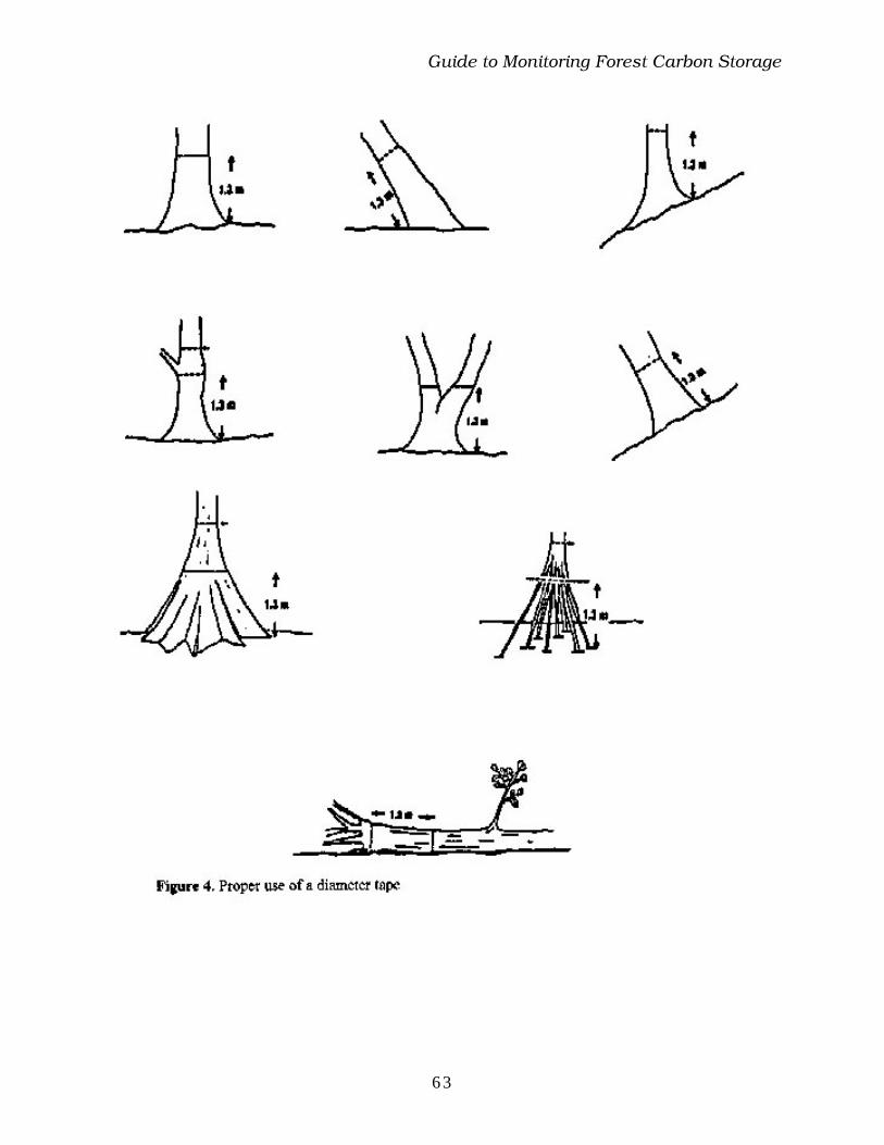
+YMHI�XS�1SRMXSVMRK�*SVIWX�'EVFSR�7XSVEKI
63
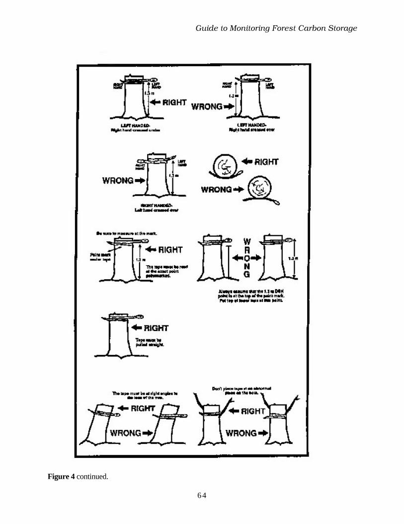
+YMHI�XS�1SRMXSVMRK�*SVIWX�'EVFSR�7XSVEKI
64
Figure 4 continued.
+YMHI�XS�1SRMXSVMRK�*SVIWX�'EVFSR�7XSVEKI
65
Appendix 5: Field Procedures for HerbaceousVegetation, Soils and Standing Litter Crop
The carbon content of soil and litter can be measured and analyzed at relatively low cost if the data iscollected at the same time the inventory is conducted. This appendix describes sampling and analysisof carbon in herbaceous vegetation, soil and standing litter crop.
In general, data should be collected in the following order:
1. Herbaceous vegetation2. Standing litter3. Soil
A. Procedure overview1. Go to the northern edge of the plot and select a point 1 m inside the outside edge of the permanentsample plot. This will be the first sampling location for herbaceous vegetation, litter and soils.
2. Lay the quadrat or circular sampling frame on the ground with the outer edge 1 m from the plotboundary. Include in the sample only the vegetation that originates inside the sampling frame.Exclude vegetation over-hanging inside the frame if the plant originates outside the frame, but includevegetation over-hanging outside the frame if the plant originates inside the frame.
3. Clip herbaceous vegetation and small woody vegetation of less than 2 cm dbh, place in the sampleweighing bag, weigh, and record the weight. Select a small random sub-sample (e.g., a handful) ofthis vegetation and place in a numbered sample bag for moisture content determination.
4. Before moving on, collect standing litter from the same sample site, place in the sample-weighingbag, weigh, and record the weight. Mix the sample well and select a small random sub-sample (e.g., ahandful) of this litter and place in a numbered sample bag for moisture content determination.
5. Collect a soil core or slice for soil carbon analysis, place this on a plastic tarp, screen with 5-mmmesh, mix well with other cores or slices, randomly select a sample, and place in a numbered samplebag for carbon content analysis.
6. Proceed in a clockwise direction to the next sampling site within the sample plot. From the firstsampling location (i.e., North) this will be East, the next will be South and the last sampling locationwill be West.
+YMHI�XS�1SRMXSVMRK�*SVIWX�'EVFSR�7XSVEKI
66
B. How many samples to collectAn inventory effort should calculate the number of samples required for a specified level of precisionbefore plot measurements begin. However, if data can be analyzed during the inventory (i.e., usingdata collected from the previous day’s collections), fewer samples may be needed. Use Form C todescribe the sampling design for soil organic carbon.
C. Herbaceous vegetationIn permanent sample plots, herbaceous understory vegetation can be sampled using four to sixquadrats or circular sample frames per plot. Figure 5 shows three types of sampling frames useful forthis type of sampling, although many alternatives exist. The main criterion is that the frames bedurable and retain their size and shape over long periods of use. All frames used in a project must beof the same size. Frames with at least one hinge allow the user to wrap the frame around broadcanopied plants when necessary. Experience suggests that round aluminum frames with hinges ontwo sides are more durable than welded square frames, and are also more easily transported.
In plotless quarter-point surveys, one quadrat should be collected at random in each quarter (seeFigure 3).
Cut all vegetation inside each quadrat/circular sampling frame at ground level. Take care to cut at thesame height for each sample. Clip herbs within the sampling frame in a vertical column extendingfrom inside the sampling frame, so that samples represent the biomass within the frame’s area. Weighbiomass for each quadrat and take and weigh a sub-sample for moisture content, and possibly fordetermining nutrient concentration.
D. Standing litter crop31
Changes in standing litter crop can be important, particularly when forest soils are converted to landuses that oxidize organic matter (e.g., crops that require intensive cultivation). It is easy to measurethe standing litter crop, but it requires consistent adherence to pre-defined standards.
Measure the standing litter crop by collecting all litter on the soil surface in each of the samplingframes used for measuring herbaceous vegetation. Samples can be bulked by plot. Make sure torecord the number of sample frames collected in each plot. Samples should be weighed and sub-samples collected in the same way as for herbaceous vegetation.
31Standing litter crop is the total weight per unit area of litter on the soil surface at the time of sampling. Litter isorganic debris on the soil surface, and is usually freshly fallen or slightly decomposed vegetation. Measurement ofthe standing litter crop does NOT require monitoring of litterfall.
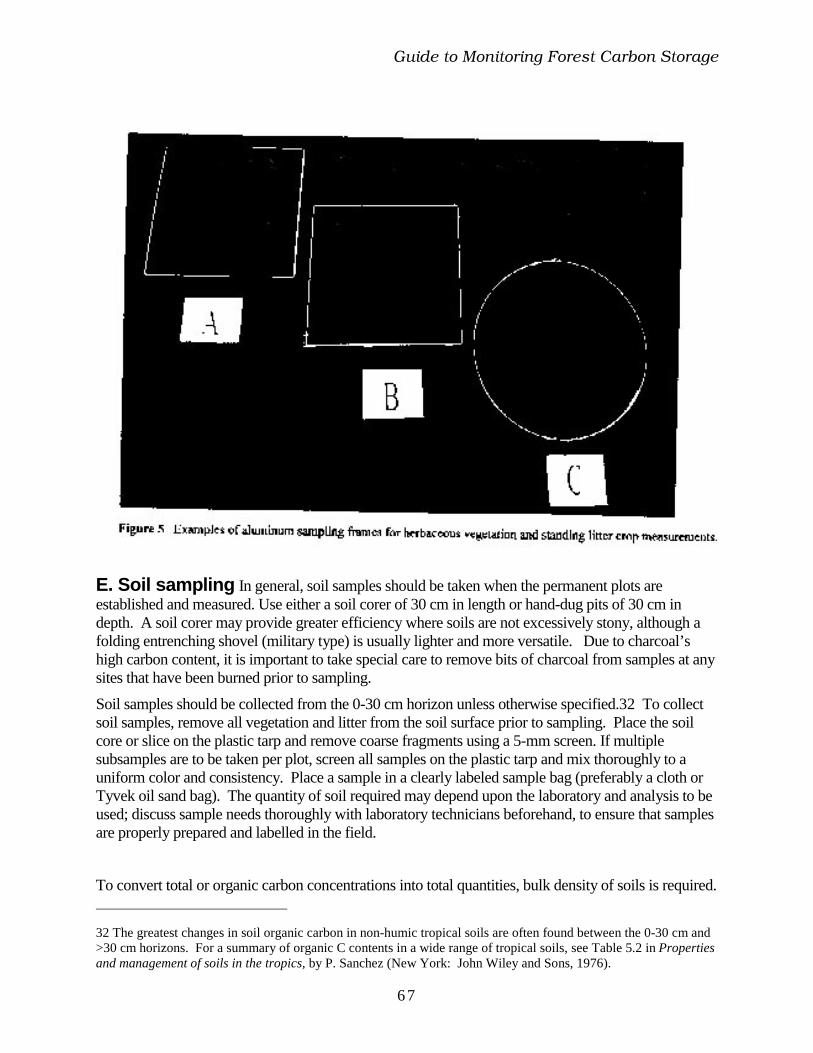
+YMHI�XS�1SRMXSVMRK�*SVIWX�'EVFSR�7XSVEKI
67
E. Soil sampling In general, soil samples should be taken when the permanent plots areestablished and measured. Use either a soil corer of 30 cm in length or hand-dug pits of 30 cm indepth. A soil corer may provide greater efficiency where soils are not excessively stony, although afolding entrenching shovel (military type) is usually lighter and more versatile. Due to charcoal’shigh carbon content, it is important to take special care to remove bits of charcoal from samples at anysites that have been burned prior to sampling.
Soil samples should be collected from the 0-30 cm horizon unless otherwise specified.32 To collectsoil samples, remove all vegetation and litter from the soil surface prior to sampling. Place the soilcore or slice on the plastic tarp and remove coarse fragments using a 5-mm screen. If multiplesubsamples are to be taken per plot, screen all samples on the plastic tarp and mix thoroughly to auniform color and consistency. Place a sample in a clearly labeled sample bag (preferably a cloth orTyvek oil sand bag). The quantity of soil required may depend upon the laboratory and analysis to beused; discuss sample needs thoroughly with laboratory technicians beforehand, to ensure that samplesare properly prepared and labelled in the field.
To convert total or organic carbon concentrations into total quantities, bulk density of soils is required.
32 The greatest changes in soil organic carbon in non-humic tropical soils are often found between the 0-30 cm and>30 cm horizons. For a summary of organic C contents in a wide range of tropical soils, see Table 5.2 in Propertiesand management of soils in the tropics, by P. Sanchez (New York: John Wiley and Sons, 1976).
+YMHI�XS�1SRMXSVMRK�*SVIWX�'EVFSR�7XSVEKI
68
Bulk density is considered to have relatively low spatial variability,33 with coefficients of variabilityof less than 10%. For a uniform soil type, four samples should be sufficient to estimate mean bulkdensity to within 10% of the true value 95% of the time. The following procedure can be used todetermine bulk density with a Modified Uhland soil corer:
1. Identify tin sample boxes and tops, weigh and record as W1 (g).
3. Prepare a smooth surface at a sampling depth of 5 cm.
4. Drive sampler into the soil to fill inner core without compression (use mineral oil if soil-metaladhesion occurs).
5. Trim ends, remove core. If core does not completely fill the cylinder, use glass bead adjustment. Ifit does fill the cylinder, push contents into sample tin, close tin, mark and record tin number.
6. Place samples in an oven set to 100o C for about 72 hours. After drying, record the weight of thetin + dry soil as W2 (g).
7. Calculate bulk density as: BD (g cm-3) = (W2-W1)/344.77
Soil C content (t ha-1 for the 0-30 cm soil depth) = BD * 300 kg m-2 * C concentration (%) * 10
F. Deciding what type of soil carbon analysis to doSoils can contain two types of carbon: organic and inorganic (carbonate). All agricultural soilscontain some organic carbon, but not all soils contain inorganic carbon. In most cases, soil organiccarbon will be the most important source of soil carbon, although this is not true in arid soils(Aridisols) and several other soil types. Most changes in soil carbon due to project activities areassumed to be in organic matter34, and not in inorganic carbonate.
Many laboratories routinely use the Walkley-Black procedure for determining soil organic carbon,although it is known to have a number of important limitations. However, because it is commonlyused, rapid, and simple, this method is recommended for analysis of soil organic carbon where totalcarbon analysis is not required. Table 5 compares methodologies for determining soil organic carbon,including Walkley-Black.
If soils are known to contain substantial quantities of inorganic carbonate and the inorganic carbonatefraction is likely to change (e.g., if an arid soil is irrigated), then total carbon methods are necessary.Table 6 provides a summary of the relative quantities of organic and carbonate soil carbon in soils, bysuborder, using Soil Taxonomy. Table 7 summarizes methodologies used for determining total soilcarbon.
33 Warrick, A.W. and D.R. Neilson. 1980. Spatial variability of soil physical properties in the field. In D. Hillel,ed., Applications of soil physics. New York: Academic Press.
34 The average C content of soil organic matter ranges from 48 to 58%.

69
Table 5 Comparison of methodologies for determining organic C in soils.
Method Principle Advantages Disadvantages
Difference between totalC and inorganic C
Total C and inorganic C are determined onseparate samples: Organic C = Total C -inorganic C.
Useful if total C and inorganic Care routinely determined
Two separate analyses are required.Total C determination requires specialequipment. Organic C calculated bydifference has some inherent error.
Determined as total Cafter removal ofinorganic C
Total C is determined in soil sample afterremoval of inorganic C with an acidpretreatment:
Organic C = Total C
Accurate if dolomite is absentfrom soil
Not all dolomite in soil may be removedby acid treatment. Specialized equipmentneeded.
Dichromate oxidationwithout external heat
Dichromate oxidizes organic C to CO2 in acidmedium. Amounts of Cr2O7
2- reduced isquantitatively related to organic C present.Not all organic C in samples is oxidized whenexternal heat is omitted, and a correctionfactor is required.
Very rapid and simple. Nospecial equipment required
Incomplete oxidation of organic Cnecessitates use of correction factors,which often results in erroneous values.Chloride, Fe2+ and MnO4 interfere withmethod. It assumes soil organic C has anaverage valence of 0.
Dichromate oxidationwith external heat
This is the same as the dichromate methodabove except that all organic C in the sampleis oxidized, and no correction factor isrequired.
Rapid and simple. Completeoxidation of organic C occurs
Chloride, Fe2+, and MnO2 interfere withmethod. Some specialized equipment isneeded. It assumes soil organic C has anaverage valence of 0>

+YMHI�XS�*SVIWX�'EVFSR�7XSVEKI
70
Table 6. Organic and carbonate carbon mass in soils of the world35
Organic Carbon Carbonate Carbon Total Carbon
Suborder/Order ---------------- Gigatons of carbon (Petagrams or 1 x 10¹⁵ g) ----------------
Folists 1 0 1
Fibrists 250 0 250
Hemists 68 0 68
Saprists 71 0 71
Histosols 390 0 390
Aquands 1 0 1
Cyrands 18 0 18
Torrands 1 1 2
Xerands 2 0 2
Vitrands 1 0 1
Ustands 13 0 13
Udands 33 0 33
Andisols 69 1 70
Aquods 4 0 4
Ferrods 0 0 0
Humods 41 0 41
Orthods 53 0 53
Spodosols 98 0 98
Aquox 1 0 1
Torrox 0 0 0
Ustox 41 0 41
Perox 16 0 16
Udox 92 0 92
Oxisols 150 0 150
Aquerts 1 1 1
Xerets 5 1 6
Torrets 12 14 26
Uderts 5 0 5
Usterts 15 9 24
35 Source: Eswaran, H., E. Van den Berg, P. Reich and J. Kimble.1995. Global soil carbon resources in R. Lal, J.Kimble, E. Levine and B.A. Stewart (Eds.). Soils and Global Change, CRC Lewis Publishers, Boca Raton, FL.

+YMHI�XS�*SVIWX�'EVFSR�7XSVEKI
71
Table 6 continued.
Suborder/Order Organic Carbon Carbonate Carbon Total Carbon
Vertisols
Salids 5 113 118
Gypsids 3 12 15
Calcids 17 407 424
Durids 0 1 1
Argids 38 112 150
Cambids 47 399 446
Aridisols 110 1044 1154
Aquults 5 0 5
Humults 4 0 4
Udults 50 0 50
Ustults 40 0 40
Xerults 2 0 2
Ultisols 101 0 101
Albolls 2 0 2
Aquolls 1 1 2
Rendolls 0 1 1
Xerolls 13 23 36
Borolls 15 29 54
Ustolls 17 32 49
Udolls 24 53 49
Mollisols 72 139 139
Aqualfs 6 0 6
Boralfs 35 0 35
Ustalfs 45 71 116
Xeralfs 14 0 14
Udalfs 36 56 92
Alfisols 136 127 236
Aquepts 67 12 79
Plaggepts 0 0 0
Tropepts 20 26 46
Ochrepts 135 247 382
Umbrepts 45 0 45

+YMHI�XS�*SVIWX�'EVFSR�7XSVEKI
72
Table 6 continued.
Suborder/Order Organic Carbon Carbonate Carbon Total Carbon
Inceptisols 267 285 552
Aquents 20 0 20
Arents 0 0 0
Psamments 21 30 51
Fluvents 3 6 9
Orthents 62 81 143
Entisols 106 117 223
Rocky land 13 0 13
Shifting sand 5 0 5
Misc land 18 0 18
TOTAL 1555 1738 3293
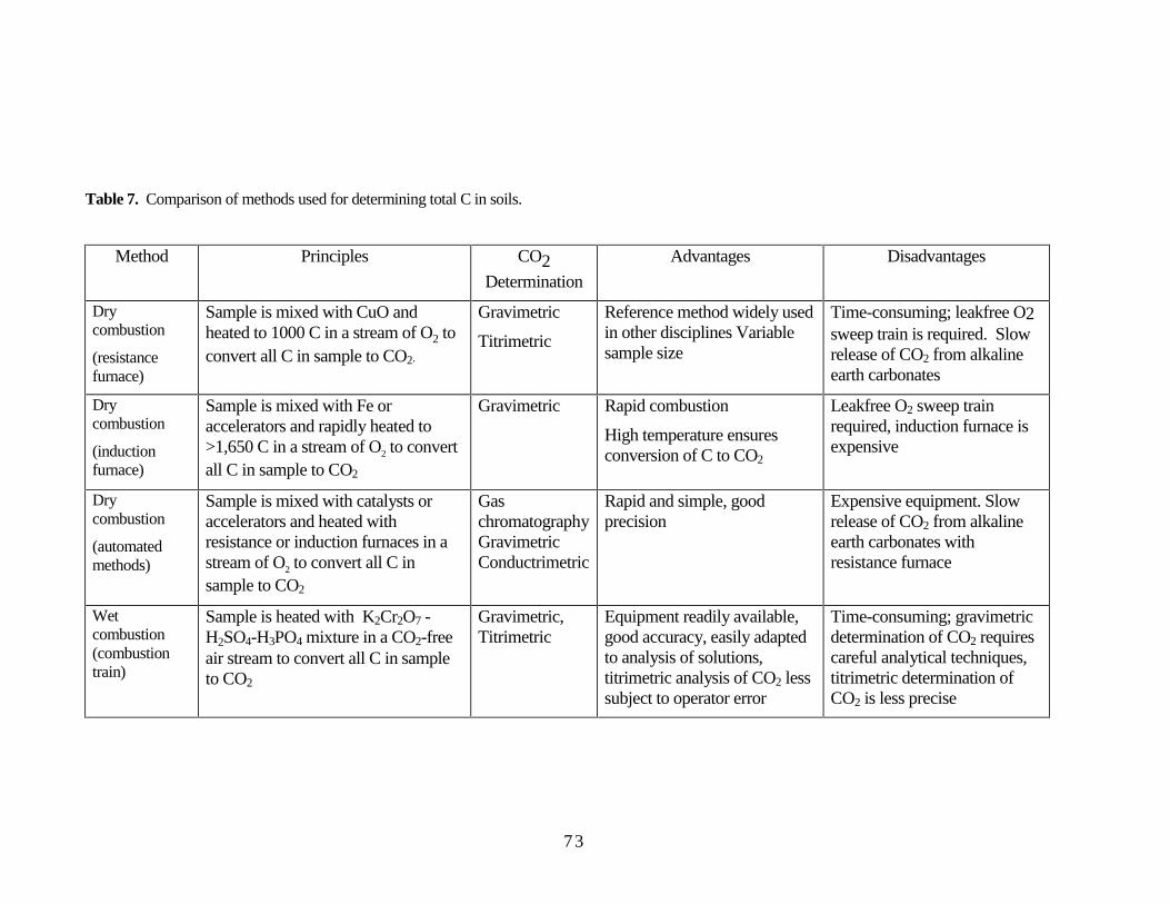
73
Table 7. Comparison of methods used for determining total C in soils.
Method Principles CO2Determination
Advantages Disadvantages
Drycombustion
(resistancefurnace)
Sample is mixed with CuO andheated to 1000 C in a stream of O2 toconvert all C in sample to CO2.
Gravimetric
Titrimetric
Reference method widely usedin other disciplines Variablesample size
Time-consuming; leakfree O2sweep train is required. Slowrelease of CO2 from alkalineearth carbonates
Drycombustion
(inductionfurnace)
Sample is mixed with Fe oraccelerators and rapidly heated to>1,650 C in a stream of O2 to convertall C in sample to CO2
Gravimetric Rapid combustion
High temperature ensuresconversion of C to CO2
Leakfree O2 sweep trainrequired, induction furnace isexpensive
Drycombustion
(automatedmethods)
Sample is mixed with catalysts oraccelerators and heated withresistance or induction furnaces in astream of O2 to convert all C insample to CO2
GaschromatographyGravimetricConductrimetric
Rapid and simple, goodprecision
Expensive equipment. Slowrelease of CO2 from alkalineearth carbonates withresistance furnace
Wetcombustion(combustiontrain)
Sample is heated with K2Cr2O7 -H2SO4-H3PO4 mixture in a CO2-freeair stream to convert all C in sampleto CO2
Gravimetric,Titrimetric
Equipment readily available,good accuracy, easily adaptedto analysis of solutions,titrimetric analysis of CO2 lesssubject to operator error
Time-consuming; gravimetricdetermination of CO2 requirescareful analytical techniques,titrimetric determination ofCO2 is less precise

+YMHI�XS�*SVIWX�'EVFSR�7XSVEKI
74
G. Sample preparationThis section describes procedures for preparing samples of soil, litter and vegetation for analysis afterthey have been collected in the field.
Soils
Soils should be air-dried, but not exposed to direct sunlight. Check with the laboratory for detailedarrangements.
Litter and vegetation
After weighing the samples, take sub-samples of litter and vegetation to determine moisture contentand nutrient concentration. The following guidelines are suggested:
Moisture content: Mix the sample and collect one random sub-sample of approximately one handfulof litter of vegetation per quadrat/circular sample plot. Bulk these subsamples by permanent plot ortransect when using the plotless method. For moisture content, collect at least five sub-samples foreach vegetation type. Sub-samples should be weighed in the field then returned to the laboratory foroven-drying at 70-80oC to a constant weight and reweighed to determine dry-matter.
Nutrient concentration: This is necessary only if the decision is made to use actual C concentrationdata for vegetation, or if actual data are to be used to predict carbon pool changes using a computermodel. A minimum of five samples for each partition is suggested for C (for carbon calculationsonly) or C and N analysis (for modelling purposes). This means five core samples of wood (collectedat dbh), five foliage and litter samples.

+YMHI�XS�*SVIWX�'EVFSR�7XSVEKI
75
Appendix 6: Measuring Carbon in Agroforestry
These methods are designed for use in agroforestry and farm forestry plantings as described in Section3. They have been only preliinarily field tested, and should be used or cited with caution (see FieldTests of Methods for Monitoring Carbon in Forestry Projects).
Map the project area.
1) Using current aerial photos, determine the number, size, and location of agroforestry plantings inthe project area. If aerial photos are not available, obtain a list of farmers who have associatedagroforestry plantings in association with the project and plot the locations of their farms to theextent possible on a topographical map.
2) Use a soils map to stratify the plantings into groups if soil types vary significantly within theproject area. If a soils map is not available for the area, consider stratification if there are majordifferences in topography, drainage, or parent material which affect the suitability of soil for cropsor trees. Avoid establishing more than three strata, if possible.
3) Assign a number to each planting within the project area.
Select a preliminary sample of plantings for the determination of required sample size.
1) Using the assigned numbers, randomly select three farms from each stratum. Measureaccumulated above- and below ground-biomass in the agroforestry plantings using the methodsoutlined below. Calculate the variance in the data, and use this value to estimate the number offarms in each stratum that must be sampled to estimate carbon accumulation at the desired level ofprecision (see Appendix 2).
2) If aerial photos are not available for the region and a preliminary estimate of averageagroforestry plantation size was not calculated, then at least six farms must be selected per stratum.The size of agroforestry plantings will be measured on each of these six farms, while three will beselected at random for the measurement of accumulated biomass. As with biomass, the variance inplanting size will be calculated to determine the number of farms that must be sampled to estimatethe average area of agroforestry plantings at the desired level of accuracy.
Select a sample of plantings for the determination of accumulated biomass.
1) Using the numbers assigned to each farm and the desired sample size calculated in the precedingstep, randomly select a sample of farms from each stratum. Make the sample list large enough sothat it includes several alternates.
2) The sampling scheme must be nested if aerial photos were not used to provide a preliminaryestimate of farm size. First, establish a random list of farms in each stratum that will be sampledfor agroforestry planting size. Next, from this list randomly select a sub-sample. Agroforestryplantations on these farms will be sampled for both size and accumulated biomass.

+YMHI�XS�*SVIWX�'EVFSR�7XSVEKI
76
3) Circle the location of the farms to be sampled on an aerial photo or topographic map. Use thismap to efficiently organize the sampling effort. Include the names of each farmer on both the mapand list of sample farms, if available.
Farmer contact
1) Before initiating field measurements, first make contact with local community leaders andofficials. Be prepared to present identification, official letters, or other forms of authorization.
2) Contact a farmer on the sample list. Formally introduce the carbon inventory crew: the names ofeach crew member, where they come from, their professional titles, and the names of theirrespective organizations.
3) Describe clearly the purpose of the carbon inventory. Do not avoid explaining why carbonsequestration is important, if asked. Describe the types of measurements that will be conducted.
4) Ask permission to inventory the accumulated biomass of the farmer’s agroforestry planting. Ifpermission is not granted, thank the family for their time, and move on to the next farm. Replacethe sample from the list of alternates.
Conduct farmer interview (see interview form, this Appendix).
Plot reference point location
1) Prepare a sketch map of the farm’s agroforestry plantings on the reference point location form.
2) Walk around the perimeter of the agroforestry planting to determine the location of each cornerof the planting with the GPS unit. Record these values on the sketch map.
3) Estimate the approximate length and width of the agroforestry planting. Record the values onthe reference point location form.
4) Divide the estimated length and width of the agroforestry planting by two. Record the values onthe reference point location form.
5) Locate the southeast corner of the agroforestry planting. Label the location of the southeastcorner on the sketch map.
6) Starting at the southeast corner and proceeding along the long side of the agroforestry plantation,measure out a line exactly equal to one half the value of the previously estimated length of theplantation (Figure 6). Use a 100 meter tape to measure this distance precisely. Record the exactdistance and bearing of the line on the reference point location form. The endpoint of this line shallbe referred to as the turn point.
7) Paint a blue ring at DBH on a tree located along the perimeter of the plantation proximal to theturn point.
8) At the turn point, turn exactly 90 relative to the direction of travel and towards the interior of theplanting. Proceed a distance exactly equal to one half of the previously estimated width of theagroforestry planting. Use the 100 meter tape to measure out this distance precisely. The endpoint

+YMHI�XS�*SVIWX�'EVFSR�7XSVEKI
77
of the line shall be referred to as the plot reference point. Record the exact distance and bearing ofthe line on the reference point location form.
9) Mark the plot reference point with a 40cm section of rebar. The bar shall be driven 30cm intothe soil, and the last ten cm of the rebar above the soil surface shall be painted blue.
10) Measure the exact distance and bearing to the plot reference point from two reference trees.Record these values on the reference point location form. The difference between the bearingsfrom the two reference trees should be approximately 90 . Paint a blue ring around each referencetree at DBH, and record the species and DBH of each reference tree on the reference point locationform.
11) Determine the coordinates of the plot reference point with the GPS. Record the coordinates onthe reference point location form.
12) Once a plot size has been selected, employ the same plot size on all plots throughout theduration of the biomass inventory, regardless of the tree spacing encountered on a particularagroforestry planting.
Plot location
1) Refer to Figure 7. If the inventory plot size is 1/20th ha or greater, the following distances andbearings shall be used to locate four plots in relation to the plot reference point (RP):
plot 1 is located 60.0 m from the RP at a bearing of 45 NE
plot 2 is located 20.0 m from the RP at a bearing of 135 SE
plot 3 is located 60.0 m from the RP at a bearing of 225 SW
plot 4 is located 20.0 m from the RP at a bearing of 315 NW
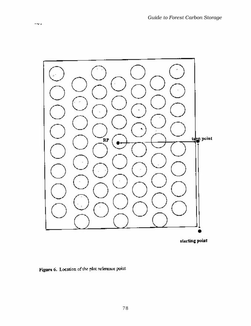
+YMHI�XS�*SVIWX�'EVFSR�7XSVEKI
78
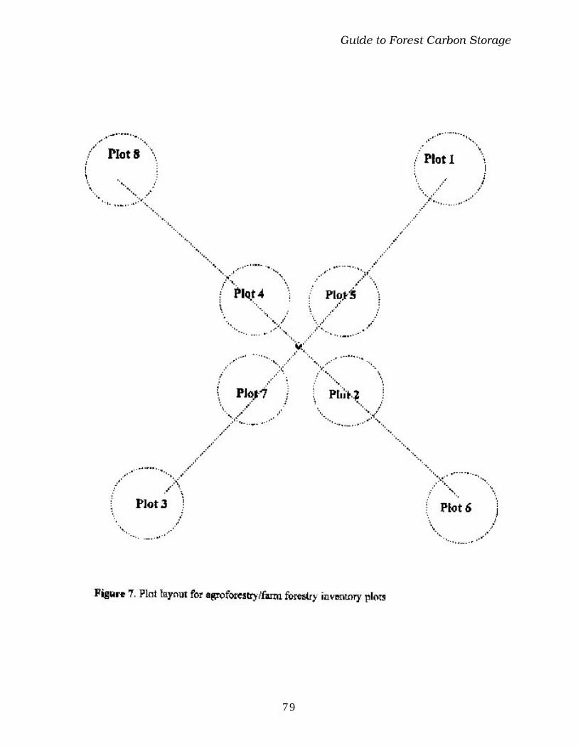
+YMHI�XS�*SVIWX�'EVFSR�7XSVEKI
79
+YMHI�XS�*SVIWX�'EVFSR�7XSVEKI
80
2) If the inventory plot size is 1/40th ha or less, use the following distances and bearings to locatefour plots in relation to the plot reference point (RP):
plot 1 is located 45.0 m from the RP at a bearing of 45 NEplot 2 is located 15.0 m from the RP at a bearing of 135 SEplot 3 is located 45.0 m from the RP at a bearing of 225 SWplot 4 is located 15.0 m from the RP at a bearing of 315 NW
3) If either the plot center or more than 25% of the plot area is located outside the perimeter of theagroforestry planting, do not establish a plot at that point. Instead, attempt to install a plot at analternate location. The first alternate is plot 5, falls outside of the agroforestry planting, then thenext alternate is plot 6, then plot 7, and finally plot 8.
4) Install the plot rope stake firmly at the center of the plot.
5) Mark the plot center with a wire flag labeled with the plot number.
Conduct an inventory of woody stems >5.0 cm DBH
1) Starting at north and moving clockwise, record the total height, DBH, and species of all woodystems > 5.0 cm DBH that fall within the plot. Record that data on the large stem biomass form.
2) For borderline trees, if more than half the stem falls within the plot, the tree is in; if more thanhalf the stem falls outside the plot, the tree is out. If the plot boundary coincides exactly with thecenter point of the tree, flip a coin. If heads, the tree is in; if tails, the tree is out.
3) The corrected slope distance should be calculated for borderline trees or for trees just outside theplot if the slope is greater than ~20%. To do this, determine the slope angle from the plot center tothe tree in question with a clinometer. Next, multiply the cosine of the angle (provided by the tableprinted on the side of the clinometer) by the apparent distance. The resulting value is the truehorizontal distance. Use this value to determine if the tree is in or out of the plot.
Conduct inventory of herbs, litter, soil and woody stems < 5.0 cm DBH (See Appendix 5)
LimitationsThe methods outlined here should be adequate for a wide array of agroforestry system configurations,but they are not appropriate for all types of plantings that may be encountered. These methods areintended for agroforestry systems which: are predominantly square, rectangular, or round in shape; atleast 0.25 hectares in size; and have trees as the predominant cover type. Narrow strips of trees, suchas windbreaks, would require a different inventory method; so would silvopastural systems in whichthe trees are widely scattered over a dominant matrix of grass. However, for most situations in whichan objective of the agroforestry project is to sequester carbon, this inventory scheme should proveadequate.

+YMHI�XS�*SVIWX�'EVFSR�7XSVEKI
81
Woody stem inventory form mo / day / year
Crew:____________________________________________ date:___/_____/____
Farm number:_______________ Stratum number:________________________________
Plot number: _______________ Plot radius: _________________
Woody stems >5.0 cm DBH
treenumber
speciescode
height DBH treenumber
speciescode
height DBH

+YMHI�XS�*SVIWX�'EVFSR�7XSVEKI
82
Farmer interview
Crew:____________________________________________ date:___/___/___
Farmer’s name: ________________________________________________________________
Farm number:_______________ Stratum number:________________________________
Farm location:_________________________________________________________________
Approximate date when agroforestry planting was established:__________________________
Land use of the plot before the planting was established:
_ fallow___ years _ pasture___ years _ crop___ years _ forest
Approximate size of agroforestry planting:___________________________________________
Reasons for establishing the agroforestry planting:_____________________________________
_____________________________________________________________________________
Tree component of the agroforestry planting:
species spacing numberplanted
growth rate problems products/ yield
Crop component of the agroforestry planting:
species spacing planting date harvest date problems products/ yield

+YMHI�XS�*SVIWX�'EVFSR�7XSVEKI
83
Reference point location form mo / day / year
Crew:____________________________________________ date:___/_____/____
Farm number:_______________ Stratum number:_________________________________
Agroforestry plantation sketch map
est. length of agroforestry plantation = ______ ÷ 2 = ______ bearing to turn pt. = _______
est. width of agroforestry plantation = ______ ÷ 2 = ______ bearing to reference pt. = _______
species DBH distance toreference pt.
bearing toreference pt.
1st reference tree
2nd reference tree
GPS coordinates of the plot reference point = ________________
+YMHI�XS�*SVIWX�'EVFSR�7XSVEKI
84
Appendix 7: Estimating Root Biomass36
Estimating root biomass is expensive. Yet, root biomass is an important carbon pool becauseit often represents 10 to 40% of total biomass. Two general approaches for claiming carboncredit for root biomass are possible: 1) use conservative, non-controversial estimates of rootbiomass based on literature values for similar vegetation types, and; 2) measure root biomass.The only advantage to measuring biomass for carbon credit is that in most cases, actual rootbiomass will likely be substantially greater than the conservative estimates. The decision ofwhether or not to measure should be based on the price of carbon compared to the cost ofcollecting the additional data required to claim credit.
A. Estimating root biomass using the literatureThe data available on root biomass are limited due to the high costs of sampling andmeasuring roots. However, the literature does contain root biomass values for a wide range ofvegetation types. Unfortunately, the methods used vary greatly and the very limitedinformation on vegetation type by site class does not allow high confidence in using actualliterature values in most cases. For example, limited root biomass data from tropical forestssuggest that the root:shoot ratio varies from 0.03 to 0.49, with below-ground biomass rangingfrom 11 to over 130 t/ha. The fact that some root biomass exists below living above-groundbiomass is undisputable, but the question is, How much? How conservative should estimatesusing literature values be? In a literature-based approach, the key is to use estimates that areconservative enough so that they are not easily refuted. In the example of the root:shoot ratioin tropical forests, a value of 0.10 or 0.15 would generally suit this purpose.
The level of conservatism required to pass minimum criteria for carbon credit is stillundefined. A reasonable approach might be to use the lowest above-ground:below-groundbiomass ratios to estimate below-ground biomass, based on actual inventory data of above-ground biomass.
B. Measuring root biomassIf such data are not available, root biomass can be estimated by sampling and measurementusing the methods described in the following paragraphs. In measuring root biomass, note thefollowing points:
• Samples should be taken from representative volumes of soil — usually 0-30 cm soil depthunless otherwise specified.
36 Portions of this appendix come from Appendix D: Roots: Length, biomass, production and mortality, byM. Van Noordwijk, in Tropical soil biology and fertility: A handbook of methods, eds. J.M. Anderson andJ.S. Ingram (London: CAB International, 1992) and Methods of studying root systems, by W. Bohm(Berlin: Springer-Verlag, 1979).
+YMHI�XS�*SVIWX�'EVFSR�7XSVEKI
85
• Samples should be taken during the time when expected standing root biomass is highest(e.g., avoid the late part of the growing season).
• The methods for sampling, storing, and washing samples will always lead to some loss ofdry weight and nutrients. A correction factor of 1.25 - 2.0 should be applied to the finaldata, with the correction factor based on the estimated losses due to sampling andprocessing.
Two types of sampling may be required: 1) core sampling to determine root biomass in the 0-30-cm soil depth; 2) monolith sampling to determine relative root distribution beyond 30 cmsoil depth. Decisions about the types of sampling required must be site specific and includeconsideration of precision needs, the availability of data on root distributions for the speciesbeing inventoried, soil depth, texture and stoniness.
Core sampling
A soil corer removes a known volume of soil from a known depth in the profile, without theneed for digging a soil pit. A core of 50 - 80 mm diameter is satisfactory, and the corer can beinserted either manually or mechanically. Manual coring is difficult at depths greater than 50cm and in clay or stony soil. In dry sandy soil a smaller core diameter may be needed toreduce losses of soil when extracting the core. In very stony soil, or where there are manywoody tree roots, coring may not be possible. In these cases, regular, known volumes of soil(monoliths) can be taken from the face of a pit and treated in the same way as cores.
A commercially available split-core corer, such as the AMS split core sampler kit with coretip, is recommended.
Ideally the profile should be sampled to the limits of rooting depth. At that depth, however,rooting intensity is low and spatial variability high. A meaningful lower limit can be set basedon initial observations of the profile wall. In some cases a linear relationship of the log of rootmass versus depth (a negative exponential root distribution) may help to extrapolate rootdensities in the soil beyond sampling depth. All soils must be sampled to a minimum depth of30 cm.
Root extraction
The best approach to root extraction is to wash roots from the cores immediately upon returnfrom the field. Core samples can be stored in sealed polyethylene bags in a refrigerator for afew days or deep freeze until processed. If deep freeze facilities are not available, samples canbe stored air-dried and re-wetted before washing. Losses of dry weight due to the methodsused for storage should be checked.
Soil texture, structure, degree of compaction and organic matter content greatly influence theprecision and time required to extract roots from cores. The simplest method involves gentlywashing a presoaked sample over a large diameter sieve of 0.3 - 0.5 mm mesh. The work canbe simplified by washing over a combination of sieves: one with 1.1 and one with 0.3 mmmesh. The first sieve will contain mostly roots, the second mostly debris. The materialremoved from the sieve(s) can then be mixed in water and the suspended material decanted(live roots of most species have a specific gravity of about 1.0). This residue should then behand sorted in shallow dishes under water to remove fragments of organic matter and deadroots; normally it is better to pick live roots from the sample and leave debris behind in thedish.
+YMHI�XS�*SVIWX�'EVFSR�7XSVEKI
86
Presoaking samples overnight in 5% sodium hexametaphosphate expedites the process ofwashing roots from clay soils, but the chemical discolors the roots (particularly in soils withhigh organic matter content) and may disrupt the tissue, making subsequent identification oflive roots more difficult. Such pretreatment will also interfere with chemical analyses. Anylengthy washing procedure may alter the element content of root tissue; only a subsamplehand sorted with a minimum of water and processed on the day of sampling should be usedfor analysis.
Classifying the roots
Fine roots are the most important part of the root system for water and nutrient uptake, as theyform the largest part of total root length or root surface area. For woody perennial vegetationthere is a fairly obvious distinction between the more or less permanent, secondarily thickenedroots and the ephemeral, unthickened roots. This functional distinction usually fallssomewhere between 1 and 3 mm root diameter. Roots above 10 mm diameter are notadequately sampled by coring. For herbaceous perennial and short-lived vegetation, rootsshould be separated into <2 mm and > 2 mm classes. In mixed vegetation, separation of rootsof different species is difficult and is not necessary.
Sampling intensity
Even in the most homogeneous soils, spatial variability of root density will be high, withcoefficients of variation in root weight commonly in excess of 40%. On heterogeneous soilsthe C.V. may be much higher. This variability implies that many replicate samples are neededif estimates of root weight need to be precise.
It is advisable to obtain reliable information at one or two well chosen situations, rather thannon-reliable data on many. Within each treatment plot take at least 3 cores. Within each plotthe samples can be pooled. In natural vegetation where there is no obvious strategy for samplestratification, take the cores on random coordinates. Where patterns are likely to occur (e.g,.row crops, alley cropping) stratification should use within row vs. between-row strata.
Monolith sampling
Monolith samples can be obtained with pinboards made by inserting U-shaped, stainless steelpins or bolts in plywood. The size of the pinboard is determined by the vegetation type, basedon previous observations, such as rooting depth and distribution and practical considerations.Soil collected with a pinboard is heavy (a sample of 100 x 60 x 10 cm of soil will weigh about100 kg), so pinboard size should be matched to the means of supporting and moving a fullpinboard. Washing away the soil exposes the roots for observation. If a coarse mesh screen isput on the pins before the board is pushed into the soil, this screen can help to keep the roots intheir original location while washing the sample. Washing the sample can be facilitated bysoaking overnight in water, deep freezing (for clay soils), soaking in oxalic acid (for soils withfree calcium carbonate) or soaking in hexametaphosphate, preferably under vacuum.Whatever the pretreatment used, gentle washing must follow.
After washing away the soil: lift the root system on the mesh screen; photograph it (on a blackcloth as background); and/or cut it according to soil layers (indicated by string between the

+YMHI�XS�*SVIWX�'EVFSR�7XSVEKI
87
pins while washing the sample), depth zones and/or distance to the plant, in order to obtainroot biomass and/or root length (see below for root length). To estimate total biomass perplant, root weight density per zone and depth has to be integrated over the relevant volume.Although the pinboard method is more time-consuming than other methods, it gives moreinformation per unit of effort spent. The method’s major weakness is that roots may break orbe displaced during washing. It is easier to distinguish between live and dead roots viapinboard sampling than in methods where the root system is not sampled in its entirety.
Assessment of root mass
Washed root samples can be stored in sealed polyethylene bags for a short time in arefrigerator, but deep-freeze storage is preferable. Oven-dry the roots and weigh. Next thedried samples should be combusted for 5 hr. in a muffle furnace in 550Û C and the residueweighed. Results should be expressed as ash-free oven-dry mass per unit volume of soil.
![Carbon Finance Possibilities for Agriculture, Forestry ... · CARBON FINANCE POSSIBILITIES FOR AGRICULTURE, FORESTRY AND OTHER LAND USE PROJECTS IN A SMALLHOLDER CONTEXT] [process](https://static.documents.pub/doc/80x56/5f96537d4b58f4729a0a77bf/carbon-finance-possibilities-for-agriculture-forestry-carbon-finance-possibilities.jpg)


