NTIAREPORT 82-100 A Guide to the Use of the ITS Irregular Terrain Model in the Area Prediction Mode G.A. Hufford A.G. Longley W.A. Kissick u.s. DEPARTMENT OF COMMERCE Malcolm Baldrige, Secretary Bernard J. Wunder, Jr., Assistant Secretary for Communications and Information April 1982
Transcript
NTIAREPORT 82-100
A Guide to the Use of the
ITS Irregular Terrain Model
in the Area Prediction Mode
G.A. HuffordA.G. LongleyW.A. Kissick
u.s. DEPARTMENT OF COMMERCEMalcolm Baldrige, Secretary
Bernard J. Wunder, Jr., Assistant Secretary
for Communications and Information
April 1982
TABLE OF CONTENTS
LIST OF FIGURES ••
LIST OF TABLES
ABSTRACT • • • • •
iv
v
1
1.
2.
3.
4.
5.
INTRODUCTION••
AREA PREDICTION MODELS. •
THE ITS MODEL FOR THE MID-RANGE FREQUENCIES •
3.1 Input Parameters3.2 General Description•.
DEVELOPMENT OF THE MODEL.
DETAILED DESCRIPTION OF INPUT PARAMETERS. •
5.1 Atmospheric Parameters.5.2 Terrain Parameters .•5.3 Other Input Parameters
1
3
5
610
14
17
182022
6. STATISTICS AND VARIABILITY••• . . . 26
7.
8.
6.1 The Three Dimensions of Variability.6.2 .A Model of Variability • • .6.3 Reliability and Confidence6.4 Second Order Statistics..
SAMPLE PROBLEMS .
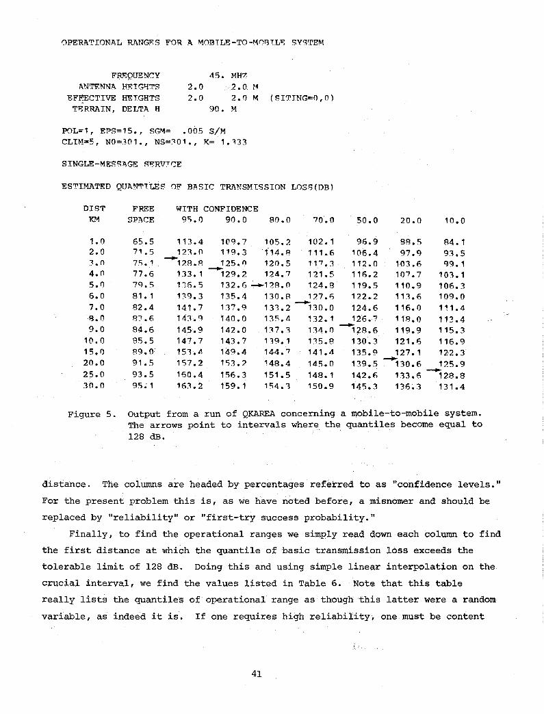
7.1 The Operating Range of a Mobile-to-Mobile System .••••7.2 Optimum Television Station Separation. • • • • •7.3 Comparison with Data . . . • . . .•.
REFERENCES. . •
28313537
38
394251
66
APPENDIX A.
APPENDIX B.
LRPROP AND AVAR--AN IMPLEMENTATION OF THE ITS MODEL FORMID-RANGE FREQUENCIES • • • • •
QKAREA--AN APPLICATIONS PROGRAM •
iii
69
101
Figure 1.
Figure 2.
Figure 3.
Figure 4.
Figure 5.
Figure 6.
Figure 7.
Figure 8.
Figure 9.
Figure 10.
LIST OF FIGURES
A typical plot of reference attenuation versus distance • • •
Minimum monthly mean values of surface refractivity referredto mean sea level • • • •.•.. • • . . • . . • . • • .
Contours of the terrain irregularity parameter ~h in meters.The derivation assumed random paths and homogeneous terrainin 50 km blocks. Allowances should be made for otherconditions. • • • • • . • • . . • • ••• • . • • • • • •
The reference attenuation versus ~h for selected distances .•
Output from a run of QKAREA concerning a mobile-to-mobilesystem. • • • •••••••••.•••.•.•...
A triangular grid of cochannel television stations showingthe arrangement of the three offset frequencies . • • • . • •
Fraction of the country receiving an interference-free signalversus the station separation. We have assumed transmittingantennas 300 m high and average terrain characteristics
The R3 data at 410 MHz; 44 points . . .
Predicted and observed values of attenuation for the R3 data.Assumed parameters: f=4l0 MHz, h 1=275 m, hg2=6.6 m,~h=126 m, N =250 N-units•••..g.••••••••.••.•
s
Predicted and observed curves of observational variabilityfor the R3 data . • • • • . . . • . • . • . • . . .
11
19
21
23
41
45
50
52
55
57
Figure 11. Predicted and observed medians for the R3indicate confidence levels for the sampleimately 10% and 90% • . • . . • . • • • •
data. The barsmedians at approx-
59
Figure 12.
Figure 13.
Figure 14.
Predicted and observed values of attenuation versus distancefor the R3 data. The predictions assumed the transmitterswere sited very carefully • • • • • • • • • • • • • • • •
The sample cumulative distribution of deviations. As indicated in the text, this is a midleading plot. • •
The sample cumulative distribution of deviations assumingthe data are censored when A ~ 0.5 dB •..••••..•
iv
61
62
64
LIST OF TABLES
Design Parameters for a SymmetriG Mobile-to-Mobile System. 40
Design Parameters for a Grid of Channel 10 Television Stations 44
Operational Ranges Under Average Environmental Conditions. 42
Table 1.
Table 2.
Table 3.
Table 4.
Table 5.
Table 6.
Table 7.
Input Parameters for the ITS ModE~l Together With the OriginalDesign Limits. . . . . . . . . .Suggested Values for the Terrain Irregularity Parameter. .Suggested Values for the Electrical Ground Constants . . . . .Radio Climates and Suggested Values for N
s
7
8
9
9
v
A GUIDE TO THE USE OF THE ITS IR~~GULAR TERRAIN MODELIN THE AREA PREDICTION MODE
*George A. Hufford, Anita G. Longley, and William A. Kissick
The ITS model of radio propagation for frequencies between 20 MHzand 20 GHz (the Longley-Rice model) is a general purpose model that canbe applied to.a large variety of engineering problems. The model,which is based on electromagnetic theory and on statistical analyses ofboth terrain features and radio measurements, predicts the medianattenuation of a radio signal as a function of distance and the variability of the signal in time and in space.
The model is described in the form used to make "area predictions"for such applications as preliminary estimates for system design, military tactical situations and surveillance, and land-mobile systems.This guide describes the basis of the model, its implementation, andsome advantages and limitations of its use. Sample problems areincluded to demonstrate applications of the model.
Key words: area prediction; radio propagat.ion model; SHF; statistics;terrain effects; UHF; VHF
1. INTRODUCTION
Radio propagation in a terrestrial environment is an enigmatic phenomenon
whose properties are difficult to predict. This is particularly true at VHF, UHF,
and SHF where the clutter of hills, trees, and houses and the ever-changing atmo
sphere provide scattering obstacles with sizes of the same order of magnitude as
the wavelength. The engineer who is called upon to design radio equipment and
radio systems does not have available any precise way of knowing what the character
istics of the propagation channel will be nor, therefore, how it will affect opera
tions. Instead, the engineer must be content with one or more models of radio
propagation--i.e., with techniques or rules of thumb that attempt to describe how
the physical world affects the flow of electromagnetic energy.
Some of these models treat very specialized subjects as, for example, micro
wave mobile data transfer in high-rise urban areas; others try to be as generally
applicable as Maxwell's equations and to represent, if not all, at least most,
aspects of physical reality. In this report we shall describe one of the latter
models. Called "the ITS irregular terrain model" (or sometimes the Longley-Rice
*The authors are with the Institute for Telecommunication Sciences, National Tele-communications and Information Administration, U.S. Department of Commerce, Boulder,Colorado 80303.
model; see Longley and Rice, 1968), it is designed for use at frequencies between
20 MHz and 20 GHz, for a wide variety of distances and antenna heights, and for
those problems where terrain plays an important role. It is concerned with the
generally available received power and not with the fine details of channel char
acterization.
On the other hand the model is avowedly statistical. In the physical world
received signal levels do vary in what appears to be a random fashion. They vary
in time because of changing atmospheric conditions, and they vary in space because
of a change in terrain. It is this variability that the model tries to describe,
thus providing the engineer estimates of not only the general level of expected
received powers but also the magnitude of expected deviations from that general
level.
Being a general purpose model, there are many special circumstances it does
not consider. In what follows we shall try to describe the general nature of the
model, to what uses it may be put, at what points special considerations might
enter, and, if we can, what steps might be taken to allow for them. The number of
possible special circumstances is so great, however, that we have undoubtedly over
looked many important ones. Here, we must depend on the ingenuity of the individ
ual engineer to recognize the circumstance and to determine how to proceed. In
general, we expect the user of this Guide to be somewhat familiar with radio propa
gation and the effects its sometimes capricious behavior will have on radio systems.
The ITS irregular terrain model is specifically intended for computer use. In
this regard it is perhaps well to introduce here terminology that makes the distinc
tions computer usage often requires. A model is a technique or algorithm which
describes the calculations required to produce the results. An implementation of
a model is a representation as a subprogram or procedure in some specific computer
language. An applications program is a complete computer program that uses the
model implementation in some way. It usually accepts input data, processes them,
passes them on to the model implementation, processes the results, and produces
output in some form. In some applications programs, radio propagation and the
model play only minor roles; in others they are central, the program being but an
input/output control. For example, the program QKAREA described and listed in
Appendix B is a simple applications program; it calls upon the subprograms LRPROP
and AVAR which are listed in Appendix A and which, in turn, are an implementation of
version 1.2.1 of the ITS irregular terrain model.
2
2. AREA PREDICTION MODELS
Most radio propagation models, especially the general purpose ones, can be
characterized as being either a "point-to-point" model or an "area prediction"
model. The difference is that a point-to-point model demands detailed information
about the particular propagation path involved while an area prediction model
requires little information and, indeed, may not even require that there be a
particular path.
To explain this latter statement, let us consider for what problems a propaI
gation model should help. There seem to be about five areas of concern:
(1) Equipment design. Given specifications of how new radio equip
ment is to be used and how reliable communications must be, it
should be possible to predict the values of path loss (and per
haps other characteristics of the channel) for which the equip
ment must compensate. Conversely, given the properties of
proposed new equipment, one should be able to predict how that
equipment will behave in various situations. In particular, one
should be able to predict a service range--Le., a distance at
which communications are still sufficiently reliable, under the
given conditions.
(2) General system design. This is an ex'tension of the first area.
Here, it is the interaction of radio equipment that is to be
studied. Often, interference, both between elements of the same
system and between elements of one system with another on the
same or adjacent frequencies, is an important part of the study.
Questions such as the proper co-channel spacing of broadcast sta
1:ions or the proper spacing of repeaters might be treated.
(3) Specific operational area. In this case one or more radio systems
are to be located in one particular area of the world and, per
haps, operated at one particular season of the year or time of
day. Within this area, however, all terminals are to be located
at random, where "random" may mean not uniformly distributed but
according to some predefined selection scheme. These terminals
may, for example, be mobile so that they will, indeed, occupy
many locations; or they may be "tactical" in that they are to be
set up at fixed locations to be decided upon at a later date,
perhaps only just before they are put. into operation. Questions
3
t6be asked might be similar to those in the previous two areas.
One technique sometimes used is that of a simulation procedure in
which a Monte Carlo approach is taken in the placement of the
terminals or the control of communications traffic.
(4) Specific coverage area. In this case, one of the terminals is at
a specific known location while the other (often many others) is
located at random somewhere in the same vicinity. The obvious
example here is a broadcast station or the base station for a
particular mobile system; but other examples might include radars,
monitoring sites, or telemetry acquisition base stations. The
usual problem is to define a service area within which the reli
ability of communications is adequate or, sometimes, to find the
strength of interference fields within the service area of a
second station. If calculations are made before the station is
actually set up, one can think of them as part of the decision
process to judge whether the station design is satisfactory.
(5) Specific communications link. In this final case, both terminals
are at specific known locations, and the problem is to estimate
the received signal level. Or more likely, the problem is to
characterize the received signal level as it varies in time.
Again, calculations made here are often used in the design of the
link.
In the last of these areas--the specific communicationslink--one knows, or
presumably can obtain, all the details of the path of propagation. One expects to
obtain very specific answers to propagation questions, and therefore one uses a
point-to-point model.
In the first two areas, however--the design of equipment and of systems--there
is no thought about particular propagation paths. One wants general results, per
haps parametric results, for various types of terrain and types of climate. It is
natural to use an area prediction model.
In the case of a specific operational area or a specific coverage area, one is
confronted with a different problem. Here one has a large multitude of possible
propagation paths each of .which can presumably be described in detail. One might,
therefore, want to consider point-to-point calculations for each of them. But the
sheer magnitude of the required input data makes one hesitant. If a simulation
procedure is used to collect statistics of communications reliability, then the
point-to-point calculations become lost in the confusion to the point where they
4
seem hardly worth the trouble. Ap.?-;J.t~rn9-tive which requires far less input data
is to use an area prediction model, particularly if the model provides by itself
the required statistics.
Even in the case of a specific communications link, the required detailed
information for the propagation path may be unobtainable so that one is forced to
use the less demanding area prediction model. Of course, in doing so one expects
to lose in precision and in the dependability of the results.
In addition to the ITS area prediction model, other widely used models of this
kind include those developed by Epstein and Peterson (1956), Egli (1957), Bulling-
ton (1957), the Federal Communications Commission (FCCi Damelin et al., 1966), Okumura
et al. (1968), and the International Radio Consultative Committee (CCIR, 1978a).
By their nature, all these models use empiricism, by which we mean they depend
heavily on measured data of received signal levels. But also, they all depend to a
greater or lesser degree on the theory of electromagnetism. In some cases, theory
is used only qualitatively to help make sense out of what is always a very wide
spread in the measured values. In others of these models theory plays a more
important role, and the empirical data serve to provide benchmarks at which the
model is expected to agree.
3. THE ITS MODEL FOR THE MID-RANGE FREQUENCIES
Originally published by Longley and Rice (1968), the ITS irregular terrain
model is a general purpose model intended to be of use in a very broad range of
problems, but not, it should be noted, in all problems. It is flexible in applica
tion and can actually be operated as either an area prediction model or as a point
to-point model. We speak here of two separate "modes" of operation. In the point
to-point mode, part of the input one must supply consists of certain "path parameters"
to be determined from the presumably known terrain profile that separates the two
terminals. In the area prediction mode these Same parameters are simply estimated
from a knowledge of the general kind of terrain involved. The two modes use almost
~dentical algorithms, but their different sets of input data and their different
ranges of application make it inconvenient to discuss them both at once. This
report treats only the area prediction mode.
In the present section we shall provide a t>rief general description of the
model inclUding its design philosophy, a list of its input parameters, and a dis
cussion of some of the physical phenomena involved in radio propagation and whether
they are or are not treated by the model.
5
Before continuing, however, we should first consider the units in which received
signal levels are to be measured. Here we come upon a confusion, for each discipline
of the radio industry se~ms to have chosen its own separate unit. Examples include
electromagnetic power flux, electric field intensity, power available at the termi
nals of the receiving ancenna, and voltage at the receiver input terminals. If one
wants to divorce the propagation channel from the equipment, one also speaks of
transmission loss, path loss, or basic transmission loss. Most of these quantities
are described by Rice et ale (1967; Section 2), but the important property to note
is that under normal conditions--when straightforward propagation takes place with
out near field effects or standing waves and when mismatches are kept to a minimum-
all these quantities are easily transformed one to another. Indeed, in this report
we use the term "signal level" so as to be deliberately vague about what precise
unit is intended, because we feel the question is unimportant.
For each of the quantities that might represent a signal level, it is possible
to compute a free space value--a value that would be obtained if the terminals were
out in free space unobstructed by terrain and unaffected by atmospheric refraction.
This free space value is a convenient reference point for radio propagation models
in general and for the ITS model in particular. Our own preference for a measure of
signal level is therefore the attenuation relative to free space which we always
express in decibels. In what follows we shall use the simple term "attenuation,"
hoping that the context will supply the reference point. The quantity is sometimes
also referred to as an "excess path loss." To convert to any other measure of sig
nal level, one simply computes the free space value in decibels relative to some
standard level and then subtracts the attenuation (adds, if one is computing a
loss).
3.1 Input Parameters
In Table 1 we list all the input parameters required by the ITS area prediction
model. Also indicated there are the allowable values or the limits for which the
model was designed. Here we shall try to define the terms involved. As it happens,
however, some of the terms are by nature somewhat ambiguous, and we shall defer more
complete descriptions to Sections 5 and 6.
The system parameters are those that relate directly to the radio system
involved and are independent of the environment. Counting the two antenna heights,
there are five values:
Frequency. The carrier frequency of the transmitted signal. Actually,
the irregular terrain model is relatively insensitive to the frequency,
and one value will often serve for a fairly wide band.
6
Table 1. Input Parameters for the ITS Model Together With theOriginal Design Limits
20 r-mz to 20 GHz1 km to 2000 km0.5 m to 3000 mvert:ical or horizontal
250 to 400 N-unitsone of seven; see Tabl~ 4
random, careful, or very careful
O.H to 99.9%
Distance. The great circle distance between the two terminals.
Antenna Heights. For each terminal, the height of the center of
radiation above ground. This may sound straightforward, and often it
is; but neither the center of radiation nor the ground '.evel is
always easy to determine. For further discussion see Section 5.
Polarization. The polarization, either vert:ical or horizontal, of
both antennas. It is assumed that the two antennas do llave the same
polarization aspect.
The environmental parameters are those that describe the environment or,more
precisely, the statistics of the environment in which the system is to operate. They
are, however, independent of the system. There are five values:
Terrain Irregularity Parameter ~h. The terrain that separates the two
terminals is treated as a random function of the distance away from
one of the terminals. To characterize this random function, the ITS
model uses but a single value ~h to represent simply the size of the
irregularities. Roughly speaking, ~h is the interdecile range of
7
Table 2. Suggested Values for the Terrain Irregularity Parameter
bh (meters)
Flat (or smooth water)
Plains
Hills
Mountains
Rugged mountains
For an average terrain, use bh=90 m.
o
30
90
200
500
The atmospheric constants, and in particular
terrain elevations--that is, the total range of elevations after the
highest 10% and the lowest 10% have been removed. further discussion
of this important parameter will be found in Section 5. Some suggested
values are in Table 2.
Electrical Ground constants. The relative permittivity (dielectric
constant) and the conductivity of the ground. Suggested values are in
Table 3.
Surface Refractivity N .s
the atmospheric refractivity, must also be treated as a random func-
tion of position and, now, also of time. For most purposes this
random function can be characterized by the single value N repre-ssenting the normal value of refractivity near ground (or surface)
levels. Usually measured in N-units (parts per million), suggested
values are given in Table 4. Further discussion will be found in
Section 5.
Climate. The so-called radio climate, described qualitatively by a
set of discrete labels. The presently recognized climates are listed
in Table 4. Together with N , the climate serves to characterize thesatmosphere and its variability in time. Further discussion is given
in Section 5.
The way in which a radio system is positioned within an environment will often
lead to important interactions between the two. DeplOyment parameters try to char
acterize these interactions. The irregular terrain model has made provision for one
such interaction that is to be applied to each of the two terminals.
Siting Criteria. A qualitative description of the care which one
takes to site each terminal on higher ground. Further discussion is
given in Section 5.
8
Table 3. Suggested Values for the Electrical Ground Constants
Relative ConductivityPermittivity (Siemens per Meter)
Average ground 15 0.005
Poor ground 4 0.001
Good ground 25 0.020
Fresh water 81 0.010
Sea water 81 5.0
For most purposes, use the constants for an average ground.
Table 4. Radio Climates and Suggested Values for N's
N (N-units)s
Equatorial (Congo)
Continental Subtropical (Sudan)
Maritime Subtropical (West Coast of Africa)
Desert (Sahara)
Continental Temperate
Maritime Temperate, over land(United Kingdom and continental west qoasts)
Maritime Temperate, over sea
360
320
370
280
301
320
350
For average atmospheric conditions, use. a Continental Temperate climateand N =301 N-units.
s
9
Finally, the statistical parameters are those that describe the kind and variety
of statistics that the user wishes to obtain. Very often such statistics are given
in the form of quantiles of the attenuation. For a discussion of this subject, and
of the meanings we like to give to the terms reliability and confidence, see Section
6.
Aside from the statistical parameters which will vary in number according to the
necessities of the problem, there are some twelve parameter values that one must
define. Although this seems a rather'long list, the user should note that in many
cases several of these parameters have little significance and may be replaced by
simple nominal values. For example, the only use to which the polarization and the
two electrical ground constants are put is to determine in combination the reflec
tivity of smooth portions of the ground when the incident rays are grazing or nearly
so. At high frequencies this reflectivity is nearly a constant. When both terminals
are more than about 1 wavelength above the ground or more than 4 wavelengths above
the sea, these three parameters have little significance, and one may as well assume,
say, "average" ground constants. At frequencies below about 50 MHz the effect of the
conductivity is dominant; otherwise the relative permittivity is the more important.
Similarly, on short paths less than about 50 km, the atmosphere has little
effect, and one may as well assume average conditions with a Continental Temperate
climate and N =301 N-units. And finally, for the siting criteria one will usuallys
assume that both terminals are sited at random. Thus, in a large proportion of
practical problems, one is left with only five parameter values to consider: fre
quency, distance, the two antenna heights, and the terrain irregularity parameter.
3.2 General Description
Given values for the input parameters, the irregular terrain model first com
putes several geometric parameters related to the propagation path. Since this is an
area prediction model, the radio horizons, for example, are unknown. The model uses
empirical relations involving the terrain irregularity parameter to estimate their
position.
Next, the model computes a reference attenuation, which is a certain median
attenuation relative to free space. The median is to be taken over a variety of
times and paths, but only while the atmosphere is in its quiet state--well-mixed and
conforming to a standard atmospheric model. In continental interiors such an atmo
sphere is likely to be found on winter afternoons during fair weather. On oversea or
coastal paths, however, such an atmosphere may occur only rarely.
10
As treated by the model, this reference attenuation is most naturally thought of
as a continuous function of distance such as that portrayed in Figure 1. As shown
there, it is defined piecewise in three regions, called the line-of-sight, diffrac
tion, and forward scatter regions. The "line-of-sight" region is somewhat misnamed;
it is defined to be the region where the general bulge of the earth does not inter
rupt the direct radio waves, but it still may be that hills and other obstructions do
so. In other words, this region extends to the "smooth-earth" horizon distance,
which is probably farther than the actual horizon distance. In this region the
reference at1:enuation is computed as a combined logarithmic and linear function of
distance; then in the diffraction region there is a rather rapid linear increase; and
this is followed in the scatter region by a much slower linear increase. Parameters
other than distance enter into the calculations by determining where the three
regions fall and what values the several coefficients have. But once the system and
its deployment (in a homogeneous environment) have been fixed, the notion of atten
uation as a function of distance should be a convenient one for many problems.
III....20
\ free spaceCIl.Q-~CIlt::l
"'CIl 40\,.
<:t
01--......
60
line-of-sight diffraction scatter
o 20 40 60 80 100 120Distance. Kilometers
140 160 180 200
Figure 1. A typical plot of reference attenuation versus distance.
11
The reference attenuation is a good representative value to indicate to a
designer how a proposed system will behave. For some problems, knowing it alone will
be sufficient. For most problems, however, one must also obtain the statistics of
the attenuation. To do this, the model first subtracts a small adjustment for each
climate to convert the reference attenuation to an all-year median attenuation.
Then from this median attenuation further allowances are subtracted to account for
time, location, and situation variability in the manner described in Section 6.
For its calculations, the model utilizes theoretical treatments of reflection
from a rough ground, refraction through a standard atmosphere, diffraction around the
earth and over sharp obstacles, and tropospheric scatter. It combines these using
empirical relations derived as fits to measured data. This combination of elementary
theory with experimental data makes it a semi-empirical model which on the one hand
should agree with physical reality at certain benchmark values of the parameters and
on the other hand should comply with physical laws sufficiently well to allow us to
interpolate between and extrapolate from these benchmark values with a good degree
of confidence. Thus the model is a general purpose one that should be applicable
under a wide variety of "normal" conditions--particularly those conditions that
correspond to the land mobile and broadcast services.
The data used in developing the empirical relations clearly have influenced the
model itself. It should then be noted that these data were obtained from measure
ments made with fairly clear foregrounds at both terminals. In general, ground cover
was sparse, but some of the measurements were made in areas with moderate foresta
tion. The model, therefore, includes effects of foliage, but only to the fixed
degree that they were present in the data used.
There are several phenomena that the model ignores, chiefly because they occur
only in special circumstances. In cases of urban conditions, dense forests, de1ib.,
erate concealment of the terminals, or concerns,about the time of day or season of
the year, it is possible to make suitable extra allowances or additions to the basic
model. This, of course, requires an engineer who knows the situation involved and
the probable magnitude of the consequent effects.
The possibility of ionospheric propagation is what makes us limit the model to
frequencies above 20 MHz. Still, there will be occasional cases of ionospheric
reflection at frequencies near this lower limit, and scatter from sporadic E will
occur at frequencies below about 100 MHz. Such effects, however, will be apparent
only on very long paths and only for very small fractions of time.
Atmospheric absorption--particu1arly the water vapor line at 22 GHz--is what
limits the model at the higher frequencies. The effects are measurable above about
12
13
terminals are sited in extreme, rather than typical, locations, the calculated atten
uation will not represent the median of measurements. An example of such an a~ypical
situation would be propagation along a narrow, steep-sided valley, where the radio
signal may be repeatedly reflected from the walls of the valley.
4. DEVELOPMENT OF THE MODEL
During the years prior to 1960, a good deal of information was obtained regarding
radio propagation through the turbulent atmosphere over irregular terrain. For
paths with fixed terminals a number of prediction models had been developed to
describe the power available at the receiver over known profiles by means of line
of-sight, diffraction, and forward scatter propagation. A good deal of data had
also been accumulated from high-powered broadcast transmitting antennas to rather
well-sited receivers. However, land-mobile types of communication systems were
becoming increasingly important. In such applications some of the terminals are
highly mobile, with randomly changing locations. Little information was available
for such systems, especially where low antenna heights and ready mobility are prime
requirements.
A theoretical and experimental program was undertaken by the National Bureau of
Standards to study propagation characteristics under conditions resembling the
operation of army units in the field. Tactical situations may often require that
antennas be low and placed as inconspicuously as possible, and that receivers be
highly mobile. A report by Barsis and Rice (1963) describes the planned measurement
program and proposed terrain analysis. The measurements were to be carried out in
various types of terrain, including the open plains of eastern Colorado, the foot
hills and rugged mountains of Colorado, and the rolling, wooded hills of north
eastern Ohio. The report describes terrain profile types in terms of a spectral
analysis which depends on a,discrete, finite-interval, harmonic analysis of terrain
height variations over the great circle path between terminals. Characteristics of
terrain profiles of any given length were described relative to a least-squares fit
of a straight line to heights above sea level.
As the study progressed, the harmonic analysis of terrain was replaced by a
single parameter bh, which is used to characterize the statistical aspects of ter
rain irregularity. Terrain statistics were developed for the areas described above
by reading a large number of terrain profiles. Each profile was represented by
discrete elevations at uniform distances of half a kilometer. Within each region
selected for intensive study, 36 profiles 60 km in length were read in each of six
directions, providing a total of 216 profiles that form a rather closely spaced grid
14
over a 100 km square area. Each profile was considered, in lengthso;f 5, 10, 20 •••
60 km to study the effects of path length on the various terrain parameters.
The interdecile range 6h(d) of terrain heights above and below a straight line,
fitted by least squares to elevations above sea level, was calculated at each of
these distances. Usually the median values of 6h(d) for a specified group of pro
files increase with path length to an asymptotic value, ~h, which is used to char
acterize the terrain. This definition of 6h differs from that used by the CCIR and
by the FCC as noted in Section 5.
An estimate of 6h(d) at any desired distance may be Obtained from the following
empirical relationship:
For homogeneous terrain, values of ~h(d)
6h (d) :::; ~h I1-0. 8 exp (-diDo)]
where the scale distance D equals 50 kID.o
measured at each distance agree well with those obtained from (1).
(1)
As the terrain
in a desired area becomes less homogeneous, the scatter of measured values of 6h(d)
increases.
For an area prediction where individual path profiles are not available, median
values of terrain parameters to be expected are calculated as empirical functions of
the terrain irregularity parameter ~h, the effec1:ive earth's radius, the antenna
heights, and the siting criteria employed.
Even at first, the model was designed to calculate the reference attenuation
below free space as a continuous function of distance. This could be easily con
verted to basic transmission loss by adding the free-space loss at each distance.
These reference values of basic transmission loss, with a small adjustment for
climate, represent the median, long-term values of transmission loss predicted for
the area.
To provide a continuous curve as a function of distance, this median attenua
tion is calculated in three distance ranges as shown in Figure 1, Section 3: a) for
distances less than the smooth-earth horizon distance dLsi b) for distances just
beyond the horizon from d to d i and c) for distances greater than d. The modelLs x xdoes not provide predictions for distances less ·than 1 km. For distances from 1 km
to dLs
, the predicted attenuation is based on two-ray reflection theory and extrap
olated diffraction theory. For distances from dLS to dx ' the predicted attenuation
is a weighted average of knife-edge and smooth-earth diffraction calculations. The
weighting factor in this region is a function of frequency, terrain irregularity,
and antenna heights. For distances greater than d , the point where diffraction andx
15
scatter losses are equal, the reference attenuation is calculated by means of a
forward scatter formulation.
In developing the original model, comparisons with data were made and empirical
relationships were established. These include expressions for calculating horizon
distances and horizon elevation angles, based on information obtained during the
terrain study. The weighting factor, used to obtain the weighted average between
rounded earth and knife-edge diffraction calculations, is based on radio data taken
from two series of measurements. The first of these provided a large amount of data
at 20, 50, and 100 MHz, obtained with low antennas in Colorado and Ohio. The
results of these measurements are reported by Barsis and Miles (1965) and by Johnson
et al. (1967). The other large body of measurements at VHF and UHF was provided to
the Television Allocations Study Organization (TASO). These measurements were made
in 1958 and 1959 in the vicinity of several cities in the United States, and the
results are summarized by Head and Prestho1dt (1960). Signals from television
stations at frequencies of about 60 and 600 MHz were measured at uniform distances
along radials with 3 and 9 m receiving antenna heights. These measurements were
made with both mobile, and stationary receivers in terrain that ranged from smooth
plains to mountains.
After the model was developed and published (Longley and Rice, 1968), compari
sons were made with a large amount of data at frequencies from 20 MHz to 10 GHz.
These comparisons are reported by Longley and Reasoner (1970). Further comparisons,
reported by Longley and Hufford (1975), were made with data at 172 MHz and 410 MHz
taken with very low antennas.
Concerning the question of statistics, recall that the original purpose was to
provide an area prediction model for land-mobile applications. Such systems involve
low antennas and low transmitter powers with consequently short ranges. For such
short paths, over land, the path-to-path variabiiity is considerably greater than
the time variability, and therefore the latter was treated rather casually. A
Continental Temperate climate was assumed and represented by a cumulative distri
bution with two slopes--two "standard deviations"--to allow for the observed greater
variability of the strong fields than of the weak ones.
As the use of the model was extended to broadcast coverage, with high power
radiated from transmitting antennas on tall towers, the effects of differences in
climate became more important in terms of possible interference between systems.
For such applications, we included sets of mathematical expressions that reproduce
the variability curves for various climates defined by the CCIR (1978b) and listed
in Table 4. Two other climates, Mediterranean and Polar, are described in the CCIR
16
Report, but curves are not presen~~d for them. For land-mobile services in the
United States, the continental Temperate climate is nearly always chosen.
The original "Longley-Rice" model was published in 1968. Shortly afterward a
new version was developed which improved the formulation for the forward scatter
prediction, and later the computer implementation was changed to improve its effi
ciency and i.ncrease the speed of operation. Since then, minor but hlportant modifi
cations have been made in the line-of-sight calculations.
To keep track of the various versions, most of which are presently being used
at some facility, we have recently begun numbering them in serial fashion. Follow
ing the original (which might be called version 0), here is a list of the more
important versions, together with approximate dates when they were first distri
buted:
1.0
1.1
1.2
1.2.1
2.0
2.1
2.2
January 1969
August 1971
March 1977
April 1979
May 1970
February 1972
September 1972
Version 1.2.1 corrects an error in version 1./.; it is the currently recommended ver
sion and is the one whose implementation is listed in Appendix A. The second series,
beginning with version 2.0, used considerably modified diffraction calculations and
tried to incorporate a groundwave at low frequencies. It is not now recommended
and is no longer maintained by its developers.
5. DETAILED DESCRIPTION OF INPUT PARAMETERS
The various parameters required as input to the ITS area prediction model were
described briefly in Section 3 of this guide. Further description and an explana
tion of their use is provided here.
The primary emphasis of the model is a consideration of the effects of irreg
ular terrain and the atmosphere on radio propagation at frequencies from 20 MHz to
20 GHz. One of the chief parameters used to describe the atmosphere is the surface
ret'ractivity Ns
' while the terrain is characterized by the parameter D.h. A discus
sion of both atmospheric and terrain parameters is presented here.
17
5.1 Atmospheric Parameters
Atmospheric conditions such as climate and weather affect the refractive index
of air and play important roles in determining the strength and fading properties of
tropospheric signals. The refractive index gradient of the atmosphere near the
earth's surface is the most important atmospheric parameter used to predict a long
term median value of transmission loss. This surface gradient largely determines
the amount a radio ray is bent, or refracted, as it passes through the atmosphere.
In this model we define an "effective" earth's radius as a function of the surface
refractivity gradient or of the mean surface refractivity N. This allows us tos
consider the radio rays as being straight so long as they lie within the first
kilometer above the earth's surface. At very much higher elevations, the effective
earth's radius assumption over-corrects for the amount the ray is refracted and may
lead to serious errors. In this propagation model we use minimum monthly mean
values of N to characterize reference atmospheric conditions. Since such values ares
less apt to be influenced by temporary anomalous conditions such as superrefraction
or subrefraction, they provide a rather stable reference which is exactly suited to
computations of the reference attenuation.
The minimum monthly mean value of N , which in the northern hemisphere oftens
corresponds to values measured in February, may be obtained from local measurements
or estimated from maps of a related parameter N. The re~ractivity N is the valueo 0
of surface refractivity that has, for convenience, been reduced to sea level.
Figure 2 from Bean et al. (1960) is a world-wide map of minimum monthly mean values
of N. The corresponding value of surface refractivity is then:o
Ns
N exp (-h /H )o s s
N-units (2)
where h is the elevation of the earth's surface and the scale height H equalss s9.46 km.
The effective earth's radius is directly defined as an empirical function of
N , increasing as N increases. It is common to set N equal to 301 N-unitsi thiss s scorresponds to an effective earth's radius of 8497 km, which is just 4/3 times the
earth's actual radius. Values of the effective earth's radius are used in computing
the horizon distances, the horizon elevation angles, and the angular distance e for
transhorizon paths.
For short distance ranges the model is not particularly sensitive to changes in
the value of surface refractivity. For this reason, in land-mobile systems we may
often assume that N has the nominal value of 301 N-units. For distances greaters
than 100 km, changes in Ns
have a definite effect on the amount of transmission
loss.18
IBO W 160 140 120 100 80 60 40 20WOE20 40 60 80 100 120 140 160 E 180
~·~r;,n~1 I 1~~N-L,.J. I j ~
~~~~J)r-r-
20
40
30
20
50
70
30
50
60
40
60
10N
oS10
70
80
5
N
80
t~r-TnITi'-i-1 I I I I I I"l--LLi_-1300
1--
300V
~
31Of.:-U lOS __ _ _ _ _ _ _ _
- - -- - '--ld~Pt=Eh;_-r
-t-
?9Ol:~.-..:~~*---t---j-t--t-f""t---=F=:f='T-I---t-----jII-t-"""I:=t=:jt::=:t=::t==t::=1-I"I'-I'""'t===-:$:=1===290CRPL BASE MAP
MODIFIED CYLINDRICAL. PROJECTION
:t;
N
80
70
60
50
40
30
20
10
N
0
I-'II~\D
20
30
40
50
60
70
80
5
180 W 160 140 120 100 80 60 40 2OWOE20 40 60 80 100 120 140 160 E 180
Figure 2. Minimum monthly mean values of surface refractivity referred to mean sea level(from Bean, Horn, and Ozanich, 1960).
Other atmospheric effects, such as changes in the refractive index and changes
in the amount of turbulence or stratification, lead to a variability in time that
may be allowed for by empirical adjustments described in Section 6.
5.2 Terrain Parameters
In VHF and UHF propagation over irregular terrain near the earth's surface, a
number of parameters are important. Early studies by Norton et al. (1955), Egli
(1957), LaGrone (1960), and others indicated that for transhorizon paths the most
important of these parameters appears to be the angular distance e. For within-the
horizon paths the clearance of a radio ray above the terrain between the terminals
is one of the most important factors.
In considering terrain effects, we usually assume that we need allow only for
the terrain along the great circle path between terminals. The angular distance eis then defined as the acute angle in the great circle plane between the radio
horizon rays from the transmitting and the receiving antennas. The angular distance
e is positive for transhorizon paths, zero at grazing incidence, and negative for
line-of-sight paths.
When detailed profile information is available for a specific path, then the
horizon distances, the horizon elevation angles, and the angular distance e may be
computed directly. In an area prediction, however, specific path profiles are not
available, and these same terrain parameters must be estimated from what we know of
the statistical character of the terrain involved. As described in Section 4,
examination of a large number of terrain profiles of different lengths in a given
area showed that median values of ~h(d) increase with path length to an asymptotic
value ~h. This parameter ~h, defined by (1), is used to characterize terrain.
We should note here that this definition of ~h differs from the one used by the
CCIR (1978a) and by the FCC (Damelin et al., 1966). Their definition is simply the
interdecile range of elevations above sea level in the range 10 to 50 km from the
transmitter. This definition results in smaller values of ~h than our asymptotic
value. We estimate that in most cases the CCIR value will equal approximately 0.64
times our value. For instance, while we would say that a world-wide average value
for ~h is about 90 m, the FCC uses the value of 50 m.
In homogeneous terrain the values of ~h(d) measured over a large number of
paths agree well with those calculated using the relationship in (1). Where the
terrain is not homogeneous, a wider scatter of values occurs, and the estimated
value of ~h(d) may not represent a true median at each distance. In such circum
stances we may allow for a greater location variability in the prediction, or at
20
times we may consider different sectors of an area and predict for each sector. An
example of this would be an area that includes plains, foothills, and mountains.
The losses predicted for each sector could be determined for the value of the ter
rain parameter computed for that sector.
The terrain parameter ~h may be obtained in one of several ways. The method
selected will depend on the purpose for which it is used and on the terrain itself.
In the original work to determine ~h for an area, a large number of profiles were
read at uniform intervals. These profiles criss'-crossed the area in such a way as
to provide a rather fine grid. The interdecile range ~h(d) was obtained for each
profile and plotted as a function of distance. The median value at each distance
was then used to obtain a smooth curve of ~h(d), whose asymptotic value is the
desired parameter ~. This method is quite laborious and may not be necessary for
the desired application. One can now use general maps of the terrain irregularity
parameter as shown in Figure 3, or one may still go directly ~o topographic maps of
the desired area and from them estimate the proper value. To do this, one may
select a random set of paths, compute the value ~h from each path, and use the
median of these calculated values to describe the terrain irregularity. with prac
tice and a few elevations read from the map, one can even estimate ~h by eye.
Figure 3. Contours of the terrain irregularity parameter ~h in meters.The derivation assumed random paths and homogeneous terrainin 50 kIn blocks. Allowances should be made for other conditions.
21
A major problem is that the area of interest is rarely homogeneously irregular.
In such a case one must exercise judgment in selecting paths that will be represen
tative of those that will actually be used in a proposed deployment. For example,
if the desired paths will always be along or across valleys, one should not choose
terrain profiles that cross the highest mountains. When virtually all paths involve
terminals on facing hillsides along the same valley, a highly preferential situation
exists.
Some qualitative descriptions of terrain and suggested values of ~h are listed
in Table 2. Whether or not one needs 'a better estimate, based on computed values,
depends on the sensitivity of the predicted values of transmission loss to changes
in ~h. This sensitivity is quite complicated, depending on the value of ~h itself,
on the antenna heights, distance range, siting criteria, and the radio frequency.
This is probably most readily illustrated by an example. Figure 4 shows plots of
attenuation relative to free space as a function of ~h at various distances. These
curves are for a land-mobile system over irregular terrain at a frequency of 150
MHz. The upper figure represents base-to-mobile communication with antenna heights
of 30 m and 2 m. The lower figure is drawn for mobile-to-mobile units with both
antennas 2 m above ground. For small values of ~h the sensitivity to change is
quite appreciable, especially at distances in the line-of-sight and diffraction
regions. Here the decrease in attenuation (a phenomenon that might be likened to
"obstacle gain") may be as much as 10 dB as ~h increases fl.'om 0 to 25 m. For
larger values of ~h from about 50 to 150 m, there is little change in attenuation
while for still larger values of ~h and for distances in the scatter region the
increases in attenuation are quite regular and less sensitive to change than for
small values of ~h.
The area prediction model depends heavily on the parameter ~h, which char
acterizes terrain, and on the surface refractivity, N. Median values of all thesother terrain parameters are computed from these two values when antenna heights are
specified. Estimates of signal variability in time and space are also dependent on
these two basic parameters. The relationships between the secondary parameters and
the terrain irregularity parameter ~h were developed mainly in rural areas where
antenna sites were always chosen with open foreground and were located on or near
roads. In these areas the ground cover was usually sparse, but some moderate
forestation was present.
5.3 Other Input Parameters
The way a system is deployed--particularly the way the terminal sites are
chosen--can have a marked effect on observed signal levels. Unfortunately, there
22
--- _d==5 km_10
V 20
----1/-30
50- -~ 75- - --L---'"" -100 -125 ---200- -
300
-- ----500-- -- -
----d==5 km
10
--------:::-- 20 --~
- 30 -50- -
V/~__- 75- -V~- 100-
125 ---
-- - 200-300_ '---
20
11\ 40.....CIIQ-lJ~
..... GOCII~
"'l
80
100o
20
11\ 40.....CIIQ-
80
100o
(a)
50
f =
50
100
150 MHz, hgl =
100
150 200i1n. Me I@rS
30 ro, hg2
= 2 ro
150 200i1n. MeIers
250
250
300
300
350
350
(b) f = 150 MHz, hgl = 2 ro,
Figure 4. The reference attenuation versus ~h for selected distances.
23
have been very few studies of these effects that could provide us with useful guid
ance. Nevertheless, the area prediction model does require the siting criteria,
which are qualitative descriptions of the care with which each 0;1; the two terminal
sites is chosen so as to improve communications. The e;l;fect of these criteria on
the model is based on reasonable assumptions, but the validity of the results has
been tested in only a limited number of examples. One should therefore exercise
caution, both in the selection of values for the siting criteria and in the inter
pretation of results.
Changes in the value of the siting criterion for one of the terminals affect
the assumed effective antenna height of that terminal. This effective height is
defined to be the height of the antenna above the "effective reflecting plane"
which, in turn, is a characterization of the intermediate foreground. It is actually
this height, not the structural height, that the model uses in nearly all of its
calculations. When the effective height increases, the model predicts less trans
mission loss and a greater communication range.
When the terminals of a system are usually sited on high ground and some
effort is made to locate them where signals appear to be particularly strong, we
say the siting is very good. When most of the terminals are located at elevated
sites but with no attempt to select hilltops or points where signals are strong, we
would classify these as good sites. Finally, when the choice of antenna sites is
dictated by factors other than radio reception, there is an equal chance that the
terminal locations will be good or poor, and we would assume the selection of
antenna sites to be random. But note that even when antennas are sited randomly we
assume they are not deliberately concealed. For concealed antennas an additional
loss should be allowed, the amount probably depending on the nature of the conceal
ment and on the radio frequency and terrain irreg~larity.
With random siting the effective antenna heights are assumed to be simply
equal to the structural heights. with good siting the effective height is obtained
by adding to the structural height an amount that never exceeds 5 m. With very
good siting the additional amount never exceeds 10 m. In both cases the actual
amount added depends on the terrain irregularity parameter, the notion being that
in more irregular terrain there will be greater opportunity to find elevated ground.
In flat areas/the effective heights will always equal the structural heights no/
matter what the siting criteria .are. The advantages achieved by good and very good
siting are greatest for low antennas with structural heights less than about 10 m.
If the antenna is on a high tower, the assumed change in effective height has
24
little significance--but it is definitely significant for antennas located just
above the ground.
The effective heights estimated from the sit.ing criteria assume that antennas
will be placed on a good site or on the best site within a very limited area. They
do not assume that antennas will be placed on the highest mountain top within a
total deployment area. But in many special problems, one will actually use just
this kind of site selection. One such problem is illustrated in Section 7.3. In
that case the receiver site was deliberately chosen at the edge of a high mesa
overlooking rather smooth terrain. This is a decidedly atypical situation. One
intuitively feels that it should be treated by setting the effective height of the
antenna equal to the height above the terrain that lies below the mesa. But in the
irregular terrain model it is the structural height that must be adjusted.
We usually define the structural height of an antenna to be the height of the
radiation center above ground. But if the antenna looks out over the edge of a
cliff, then it seems entirely natural to say that the cliff is really a part of the
antenna tower and to include its height in the structural height. Another, more
common, example of this same problem occurs in the design and analysis of VHF and
UHF broadcast stations. There, it is the usual practice to site the antenna atop a
hill or well up the side of a mountain in order to gain a very definite height
advantage. While we no longer have an obvious cliff, this height advantage should
still be accounted for by including it in the structural height.
There are several rules used by various people to determine what the ground
elevation should be above which the antenna height is to be found. The FCC uses
the 2 tolD mi (3 to 16 km) average elevation for the radial of interest. Another
rule that has been suggested is that one should not coUfit as "ground" anything that
has a depression angle from the center of radiation of more than 45°. In our own
work we have sometimes said that consideration of terrain elevations should begin
at a point distant about 15 times the tower height.
The choice of a radio climate may be difficult or confusing for the reader.
The several climates described by the CCIR have not been mapped out as various
zones throughout the world, and there are no hard and fast rules to describe each
of the climates. Since our model is intended for use over irregular terrain, our
preference is to use the Continental Temperate climate unless there are clear
indications to choose another. The CCIRcurves showing variability in time are
entirely empirical and depend on the climate chosen. The curves for Continental
and Maritime Temperate climates are based on a considerable amount of data, while
those for the other climates depend On much smaller data samples. The Continental
25
Temperate climate is common to large land masses in the temperate zone. It is
characterized by extremes of temperature and pronounced diurnal and seasonal changes
in propagation. In mid-latitude coastal areas where prevailing winds carry moist
maritime air inland, a Maritime Temperate climate prevails. This situation is
typical of the United Kingdom and of the west coasts of the United States and
Europe. For paths that are less than 100 km long, there is little difference
between the Continental and Maritime Temperate climates, but for longer paths the
greater occurrence of superrefraction and ducting in maritime areas may result in
much higher fields for periods of 10 percent or less of the year.
In considering time variability, it is important to note that we are concerned
only with long-term variability, the changes in signal level that may occur during
an entire year. The data on which such estimates are based were median values
obtained over short periods of time, an hour or less. The yearly signal distri
butions are then distributions of these medians. This eliminates much of the
short-term variability, which is usually associated with multipath. The rapid,
short-term, mUltipath fading at a mobile receiver depends on many local factors
including the type of receiving equipment, reflections from buildings and trees,
and the speed at which the recording vehicle travels. In smooth, uncluttered ter
rain there may be little if any multipath fading, whereas the most severe fast
fading is Rayleigh distributed. Even simple diversity techniques will greatly
reduce this short-term multipath type of fading.
6. STATISTICS AND VARIABILITY
We come now to a discussion of how the ITS irregular terrain model treats the
statistics of radio propagation. As we have mentioned before it seems undeniable
that received signal levels are subject to a wide variety of random variations and
that proper engineering must'take these variations into account. Unfortunately,
the problem is considerably more complicated than problems of simple random vari
ables one encounters in elementary probability theory.
The principal trouble is that the population of observed signal levels is
greatly stratified--i.e., not only do the results vary from observation to observa
tion (as one would expect) but even the statistics vary. Now it is not surprising
that this should be the case when one varies the fundamental system parameters of
frequency, distance, and antenna heights; nor is it surprising when one varies the
environment from, say, mountains in a continental interior to flat lands in a
maritime climate, or from an urban area to a desert. But even when such obvious
26
parameters and conditions are accounted for, thE~re remain many subtle and important
reasons why different sets of observations have different statistics.
Our problem here is analogous in many ways to that of taking public opinion
polls. There results depend not only on the qUE!stions asked but also on many
subtleties concerning how, where, and when the questions are asked. If one spends
the working day telephoning people at their homes, then one obtains the opinions of
those people who own telephones and answer them and who have remained at home that
day. This procedure might still be a random sampling and might, indeed, provide
acceptable results, if it were not for the fact that public opinion is, again,
greatly stratified--i.e., that the opinions of one segment of the population can
differ greatly from those of another.
In the case of radio propagation, it is the equipment and h9w, where, and when
it is used that provides an added dimension of variability. Perhaps one or both
terminals are vehicle mounted and constrained to streets and roads. Perhaps,
instead, one antenna is likely to be mounted on a rooftop. Perhaps it is most
probable that both antennas are well removed from trees, houses, and other obsta
cles; or perhaps it is likely that one of the antennas is close to such an obstacle
or even inside a building, whether this be for convenience or because concealment
is desirable. It may be that two regions of the world appear, even to the expert's
eye, to offer the same set of impediments to radio propagation and yet the differ
ences--whose effects we do not understand--may be important.
In any case, the way in which equipment is deployed has an often important
and unpredictable effect on observed signal levels. We propose here to use the
word situation to indicate a particular deployment, whether in actual use or simply
imagined. In technical terms, a situation is a probability measure imposed on the
collection of all possible or conceivable propagation paths and all possible or
conceivable moments of time. (A good introduction to the theory of probability
measures is given by Walpole and Myers, 1972, Ch. 1.) To choose a path and a time
"at random" is therefore to choose them according to this probability measure.
Insofar as ,ve want to get below the level at which stratification is important, we
would want 1:0 restrict a situation (that is, to restrict the set of paths and times
where the imposed probability is non-zero) to include only paths with a common set
of system parameters, lying within a single, homogeneous region of the world. This
is a natural restriction except, perhaps, as it affects the distance between termi
nals. The distance is a parameter which is difficult to fix while still allowing
a reasonable selection of paths.
27
If we are concerned with a single, well-defined communications link with fixed
terminals, then the situation involved has only a single isolated path which is to
be chosen with probability one. But the deployment of a land-mobile system in one
single area would define a more dispersed situation. Note, moreover, that if the
mobile units pass from an urban area to a suburban or rural area, then we would
suppose they pass from one situation to another. If one sets out to make a set of
measurements of received signal levels, then one will sample from what is, if the
measurement program has been properly designed, a situation pre-defined by the
program objectives. Often the measurements will be in support of what will become
a system deployment. It is then always proper to ask whether the situation from
which the data are taken corresponds accurately enough to the situation in which
the system will operate.
Once again, all this fussiness would be unnecessary--and radio propagation
engineering would long ago have become a finely honed tool--if it were not that the
population of received signal levels is a stratified one. The system parameters,
the environmental parameters, and the situation in which one is to operate are all
important and each of them has some effect on the final statistics. The complexity
of nature often forces us to empirical studies of these statistics; but the large
number of dimensions involved makes this a difficult task.
6.1 The Three Dimensions of Variability
We turn now to a general discussion of the physical phenomenology involved.
First, we should note that there is a very important part of the variability that
we do not wish to include. This is the short-term or small displacement variability
that is usually attributed to multipath propagation. Although it is probably the
most dramatic manifestation of how signal levels vary, we exclude it for several
reasons. For one, a proper description of mult~ath should include the intimate
details of what is usually known as "channel characterization," a subject that is
beyond our present interests. For another, the effects of multipath on a radio
:;;ystem depend very greatly on the system itself and the service it provides. Often
a momentary fadeout will not be of particular concern to the user. When it is, the
system will probably have been constructed to combat such effects. It will use
redundant coding or diversity. Indeed, many measurement processes are designed so
a:;; to imitate a diversity system. On fixed paths, where one is treating the
received signal level as a time series, it is common to record hourly medians-
i.e., the median levels observed during successive hours (or some comparable time
interval). We may liken the process to a time diversity system. If measurements
28
are made with a mobile terminal, one often reports on selected mobile runs about
30 m in length. Then, again, one records the median levels for each run, thus
simulating a space diversity system. Under the "frozen-in-space" hypothesis con
cerning atmospheric turbulence, one expects hourly medians and 30-m run medians to
be about the same. (But the analogy becomes rather strained for mUltipath in urban
areas.) To the two measurement schemes above, it would seem reasonable to add a
third to correspond to frequency diversity. This would be a "wideband" measurement
in which the average or median power over some segment of the spectrum were recorded.
In any case, it is only the variation of these local medians that concerns us.
If one still finds it necessary to consider instantaneous values of cw signals,
then the usual practice is simply to tack on an additional variability to those we
shall describe here. Often, one assumes either that the signal is locally steady
(in areas where there is no multipath) or that it is Rayleigh distributed (in areas
with extreme multipath). Occasionally one will assume an intermediate case, using
the Nakagami-Rice (see, e.g., Rice et al., 1967, Annex V) distributions or the
Weibull distributions.
If we set out to measure statistics of local medians, the first step that
occurs to us is to choose a particular fixed link and record measurements of hourly
median received signal levels for 2 or 3 years. The resulting statistics will
describe what we call the time variability on that one path. We could characterize
these observations in terms of their mean and standard deviation; but, both because
the distribution is aSYmmetric and not easily classified as belonging to any of the
standard probability distributions, and because the practicing engineer seems to
feel more comfortable with the alternative, we prefer to use the quantiles of the
observations. These are the values not exceeded for given fractions of the time
and are equivalent to a full description of the cumulative distribution function as
described in the elementary texts on statistics. We would use such phrases as "On
this path for 95% of the time the attenuation did not exceed 32.6 dB."
If we now turn our attention to a second path, we find to our dismay that
things have changed. Not only are individual values different, as we would expect
given the random nature of signal levels, but even the statistics have changed. We
have a "path-to-path" variability caused by the fact that we have changed strata in
the population of observable'signal levels. Suppose, now, that we make a series of
these long-term measurements, choosing sample paths from a single situation. In
other words, we keep all system parameters constant, we restrict ourselves to a
single area of the earth and keep environmental parameters as nearly constant as is
reasonable, and we choose path terminals in a single, consistent way. We still
29
find that the long-term time statistics change from path to path and the variation
in these statistics we call location variability. Of course, if the situation we
are concerned with has to do with a single, well-defined link, then it is improper
to speak of different paths and hence improper to speak of location variability.
But in the broadcast or mobile services, it is natural to consider such changes.
The most obvious reason for the observed variability is the accompanying change in
the profile of the terrain lying between the two terminals; although the outward-
statistical, so to speak--aspects of t]le terrain may remain constant, the actual
individual profiles, together with other, less obvious, environmental changes, will
induce large changes in observed signal level statistics.
If we try to quantify location variability, we must talk of how time variabil
ity varies with path location. We have no recourse but to speak of the statistics
of statistics. Clinging to the terminology of quantiles, we would speak of quan
tiles of quantiles and come up with some such phrase as "In this situation there
will be 70% of the path locations where the attenuation does not exceed 32.6 dB for
at least 95% of the time."
Finally, we must ask what effect there is when one changes from situation to
situation. It should be no surprise to be told that the statistics we have so
painfully collected following the outline above have changed. If we use like
appearing situations--that is, if we change operations from one area to another
very similar area or if we merely change the sampling scheme somewhat--then the
observed changes in the location variability we call situation variability.
In other contexts this last variability is sometimes referred to as "predic
tion error," for we may have used measurements from the first situation to "predict"
the observations from the second. We prefer here to treat the subject as a manifes
tation of random elements in nature, and hence as something to be described.
To make a quantitative description however, we must renew our discussion of the
character of a "situation." We have defined a situation to be a restricted proba
bility measure on the collection of all paths and times. But if we are to talk of
changing situations--even to the point of choosing one "at random"--then we must
assume that there is an underlying probability measure imposed by nature on the set
of all possible or conceivable situations. And we must assume that at this level we
have specified system parameters, environmental parameters, and deployment param
eters in sufficient detail so that the variability that remains is no longer strat
ified--in other words, so that any sample taken from this restricted population will
honestly represent that population. It is at this point that "hidden variables"
enter--variables whose effects we do not understand or which we simply have not
30
chosen to control. The values of these variables are at the whim of nature and
differ between what would otherwise be identical situations. The effects of these
differences produce the changes in observed statistics.
We are now at the third level of the statistical descr;iption, and evidently we
must speak of quanti1es of quantiles of quantiles.. This produces the phrase, "In
90% of like situations there will be at least 70!~ of the locations where the atten
uation will not exceed 32.6 dB for at least 95% of the time."
In general terms such quanti1es would be represented as a function A{'tr,qL,qS)
of three fractions: 'tr' the fraction of time; qL' the fraction of locations; and
qs' the fraction of situations. The interpretation of this function follows the
same pattern as given above: In qs of like situations there wi1~ be at least qL of
the locations where the attenuation does not exceed A(~,qL,qS) for at least qT of
the time. Note that the inequalities implied by the words "at least" and "exceeds"
are important reminders that we are dealing here with cumulative distribution
functions. Note, too, that the order in which the three fractions are considered is
important. First, one chooses the situation, then the location, and finally the
time.
We recall that if a proposition is true with probability q then it is false
with probability 1-q. Working our way through all the inequalities involved, we may
also say: In l-qs of like situations there will be at least l-qL of the locations
where the attenuation does exceed A(qT,qL' qs) f,or at least 1-qT of the time. This
is the kind of phrase one uses when trying to avoid interference.
6.2 A Model of Variability
As complicated as it is, the three-fold description of quantiles does not
completely specify the statistics. At the first level when we are considering time
variability it is sufficient. But at the very next level we have failed to notice
that we are trying to characterize an entire function of quantile versus fraction
of time qT. To do this completely, we would need to consider all finite sequences
qT1' 'tr2' .•• of fractions of time and to examine the resulting observed quantiles
all at once as a multivariate probability distribution. At the third and final
level, matters become even worse.
Obviously this becomes too complicated for practical applications; nor would a
study following such lines be warranted by our present knowledge. But there are
engineering problems that arise which can be aided by a more complete description
of these statistics. Implicit within the ITS irregular terrain model is a second
model which concerns variability and which can tIe used to provide such a descrip
tion. It is a relatively simple model using a combination of simple random variables
31
each of which depends on only one of the three different dimensions of variability.
While retaining the features described in the p:r;-evious paragraphs, it allows the
engineer to derive formulas for many needed statistics.
Experience shows us that when signal levels are expressed in decibel notation
the observed distributions tend to be normal or at least approximately normal. It
is from this fact that inspiration for the model is largely derived. The broad
statement of normality does, however, suffer from one important flaw which appears
when we discuss signal levels that exceed free space values. Such signal levels
are possible and are, indeed, observed; but their occurrence is rare and becomes
increasingly more rare as one considers ever higher levels. The distributions we
obtain must be truncated or heavily abbreviated at levels above free space.
As it happens, the terminology the ITS irregular terrain model uses to describe
the magnitude of variability differs in a slight way from that used above. As in
Rice et al. (1967, Annex V), the model considers the positive direction of a
deviation as an increase of signal level rather than of attenuation or loss. There
is, of course, no real significance to this convention, but the introduction of an
extra minus sign does tend to confuse our subsequent arguments. For this one
section, therefore, we shall adopt a different posture. Using lower-case letters
to refer to random variables, we suppose that the object of concern is the signal
level w which we measure in a decibel scale. We leave the precise definition of
this signal level deliberately vague, since it is immaterial here whether we speak
of power density, field strength, receiver power, or whatever. It would be related
to the attenuation a by the formula
w = W - afs(3)
where Wfs ' which is not a random variable, is the signal level that would be
obtained in free space.
The above change in convention requires a slight change in our definition of a
quantile. To retain the same relations as are used in practice, we now say it is
the value which is exceeded for the given fraction. For example, if w were a
simple random variable, we would define the quantile W(q) as being the value which
w exceeds with probability q. We should perhaps refer to this as a "complementary"
quantile, but instead we shall merely depend on the context to determine the implied
inequality. The rule to remember he:r;-e is that we assume the attitude of trying to
detect a wanted signal. It must be sufficiently large with a sufficiently high
probability.
32
Our model of variability is a mathematical representation of how one is to
view the received signal level as a random variable. First we assume the system
parameters, the environmental pa~~~ters, and the deployment parameters have been
fixed. From the set of all situations with thesc~ parameters, we choose at random a
particular one s. Then using that situation (which is, remember, a probability
measure) we choose at random a location ~ and a time t. The triple (t,~,s) forms
our elementary event, and the corresponding received signal level w(t,~,s) becomes
a random variable. The model expresses this function of three variables in a more
explicit and manageable way. We first define a tentative value of the signal
level
w' (t,~, s) = Wo + YS (s) + 0L (s) YL Cit) + 0T (5) YT (t) (4)
where Wo is the overall median signal level; yS' YL' YT are thr~e random variables
called deviations; and 0L' 0T are another two random variables called multipliers.
The three deviations are measured in decibels and their median values are a dB.
The two multipliers are dimensionless, always positive, with medians equal to
unity. We now come to the important assumption that the five random variables here
are all mutually independent. This enables us to treat each of them separately and
then to combine them using standard probability theory.
The final step in our model is to write
w(t,~,s) = M(w' (t,~,s» (5)
where M is a modifying function which corrects values greater than the free space
value. For values of w' less than the free space value, we set M(w')=w'; but
otherwise M puts an upper limit on values Qr at any rate reduces them considerably.
As presently constituted, the ITS irregular terrain model cuts back the excess over
free space by approximately a factor of 10. Thus, if Wfs is the free space value
of received signal level, we have M(w') ~ 0.9 Wfs + 0.1 w' when w' > Wfs·
The statistics of the three deviations and the two multipliers depend on the
system parameters, the environmental parameters, and the deployment parameters.
Except that the two multipliers must be positive, the five random variables are
approximately normally distributed. The deviations have standard deviations on the
order of 10 dB, while the multipliers have standard deviations equal to 0.3 or less.
The actual values have been derived from empirical evidence and engineering judg-
mente
Using this model we can, for example, recov'er the three-dimensional quantiles
discussed previously by following the prescribed procedure step by step. At the
33
first step we would assume there is a fixed situation and a fixed location at which
we observe the received signal level as a function of time. Now one very useful
property of quantiles has to do with the composition of random variables with mono
tonically increasing functions. If, say, u is a random variable with quantiles U(q)
and if F is a monotonically increasing function, then, as one can easily show, the
random variable F(u) has the quantiles F(U(q». Since 0T(s) is positive, the right
hand side of (4) is a monotonically increasing function of YT' and therefore the
time variant quantiles are given by
(6)
where YT(qT) is the ~ quantile of YT. At the next step we would have a fixed
situation and a fixed time variant quantile, and we would look at (6) as a function
of location alone. Again, if YL(qL) is the qL quantile of YL' we quickly find what
is now a twofold quantile
(7)
At the third step we must consider (7) as a random variable since the situation s is
now to be chosen at random. But here we have a new problem. The right-hand side of
(7) is the sum of a fixed number Wand three mutually independent random variables.o
The statistics of W2must therefore be computed from the convolution of the corre-
sponding three probability distributions. When this has been done, we would pick
off the desired quantile and finally come upon the threefold expression W' (qT,qL,qS).
In the last step, we recall that the modifying function M is monotonically increasing
and so
(8)
The only difficult part in this sequence of computations appears when we must
find the convolution required by (7). To do this the ITS irregular terrain model
uses an approximation sometimes called pseudo-convolution. This is a scheme described
by Rice et aL (1967) to treat several applications problems where the sum of inde
pendent random variables is concerned. For completeness and because it is useful in
many applications of the model, we pause here to provide our own description.
In the general case we would have two independent random variables u and v with
corresponding quantiles U(q), V(q). We then seek the quantiles W(q) of the sum
w=u+v. We first form the deviations from the medians which we recognize as having
quantiles
34
Yu(q) = U(q) - U(0.5)
YV(q) = V(q) - V(0.5)
and then we simply use a root-sum-square to derive
W(q) ;:::: U(0.5) + V(0.5)
(9)
+ sign(0.5-q) (10)
If u and v are normally distributed, this expression is exact. For other distribu
tions we can only say that results are reasonable and that in our own experience
using distributions that arise naturally in the applications the expression is sur
prisingly accurate. It is, however, meant to be only an approximation and must
always be treated as such.
Note that the extension of (10) to more than two summands is straightforward.
The expression even shares with actual convolution the property of being associative
and commutative so that the order in which summands are combined is immaterial.
6.3 Reliability and Confidence
The use of the three-dimensional quantiles is perhaps best illustrated by its
application to the broadcast services. A broadcaster will need to provide an
adequate service to an adequate fraction of the locations at some given range. But
"adequate service" in turn implies an adequate signal level for an adequate fraction
of the time. For television channels 7 to 13, for example, in order to provide
Grade A service the broadcaster must deliver (O'Connor, 1968) a field strength 9 m
above the ground which exceedes 64 dB~ for more than 90% of the time, and that in
at least 70% of the locations. Spectrum managers and also the broadcast industry
will in turn want to assure that a sufficient fraction of the broadcasters can meet
their objectives. If we assume that each broadcaster operates in a separate
"situation," then this last fraction is simply a quantile of the situation vari
ability.
For other services, however, it is often difficult to see how the three
dimensional quantiles fit in, and indeed it is probably the case that they do not.
Consider again the broadcast service. A single broadcaster will want to know the
probability with which a given service range will be attained or exceeded. Since
"service range" involves specified quantiles of location and time, the probability
sought concerns situation variability and we return to three-dimensional statistics.
35
On the other hand, consider the same problem from the point of view of an individual
receiver. That individual will want to know only the probability at that one
location of receiving adequate service--that is, of receiving an adequate signal
level for an adequate fraction of the time. The distinction between location vari
ability and situation variability will be of no concern and should not enter into
our considerations.
Using our model as in (4) and (5) we quickly note how we can accommodate a new
kind of analysis. We can suppose that first both the situation and the location
are chosen simultaneously and then, second, the time. The first choice will have
said that all four random variables in (4), excepting only YT' are to be treated at
once and are to be combined into a single deviation yS + cL YL and a single multi
plier cT' What we would have remaining is a twofold description of variability
involving time variability and a combined situation/location variability, and this
is precisely the description that the individual receiver of a broadcast station
would find useful.
To .continue our discussions, we find it convenient here to introduce the term
reliability. This is a quantile of that part of the variability which enters into
the notion of "adequate service." For the individual receiver of a broadcast
station, reliability is concerned with a fraction of time. For a broadcaster,
however, reliability must be expressed as a twofold quantile involving time and
location variability separately. For the remaining variability--always at a higher
level in the hierarchy--we use the term confidence; and we mean this term in the
sense that if one makes a large number of engineering decisions based on calcula
tions that use the same confidence level, then, irrespective of what systems or
even what types of systems are involved, that same fraction of the decisions should
be correct--and, of course, the remainder should be incorrect. Reliability is a
measure of the variability that a radio system will observe during the course of
its deployment. Confidence will be moasureable only in the aggregate of a large
number of radio systems. Clearly, differentiation between the two will depend on
the point of view one takes. To a broadcaster, confidence will be a measure of the
situation variability; to an individual receiver of a broadcast station, it will be
a measure of a combined situation and location variability. But the spectrum
planner of the broadcast service will not speak of confidence at all; from that
point of view all of the variability is observable and is part of the system.
Remembering that we must retain the order in which the three kinds of vari
ability appear, there are four different ways that one can treat them in combination,
all of which have legitimate uses in one kind of service or another. We call these
36
the four modes of variability, although they are really four different ways of
treating the subject of variability.
Two of these four modes we hav~ ~~+eady discussed. In the broadcast mode we
treat all three kinds of variability separately. The typical user of this mode
would be the broadcast~r for whom reliability would measure both location and time
variability and confidence would measure situation variability. In the individual
mode situation and location variability are combined so that there remain this com
bined variability and time variability. Here, the typical user would be the
individual receiver of a broadcast station for whom reliability means the time
availability, and confidence measures the combined situation/location variability.
It would also be legitimate to combine location and time variability. We call
the result the mobile mode, since to a mobile radio unit changes in location
translate into changes in time. The typical user of this mode would be a mobile
system employing a single base station. Reliability would refer to the combined
location/time variability; it would probably translate into fraction of attempts at
establishing communications. Confidence would be a measure of the situation
variability.
Finally, in the single message mode we combine at once all three of the kinds
of variability, thus obtaining the more usual sort of one-dimensional random vari
able. The statistics to be used here are much simpler than those we have been
discussing; but, we think, the useful applications are somewhat limited. One
application might be for a communications link that will be used but once. Examples
might include a disaster warning system or a radio link attached to a self-destruc
ting device. The statistics involved would then be couched in terms of confidence
levels. A more important application, however,would be for a mobile-to-mobile
system where the two mobile units are to be deployed worldwide. The statistics
would translate into first-try success probabilities (Hagn, 1980) and thereby
become expressions of reliability.
6.4 Second Order Statistics
Until now we have been discussing only first order statistics--that is, the
statistics of received signal levels for a single path at a single time. But there
are many problems in which more needs to be known. These are problems that depend
on the relative signal levels on separate paths or at separate times. For example,
the problem of interference comes first to mind. Also, there is the question of
37
what happens on~uccessive hops in a chain of communication links, or how to treat
the connectivity of a network of repeaters such as has been suggested for military
use.
The resolution of such problems depends on second or higher order statistics
where one considers the joint probabilities of obtaining given signal levels over
two or more paths. The most common statistic employed here is the correlation
coefficient, but in the general case one might well be forced to use something more
complicated.
Unfortunately, almost nothing is known about the subject. There have been
studies concerning diversity systems in which correlation coefficients have been
found for the two time series obtained when two receiving antennas are separated by
only a few wavelengths or in frequency by only a small fraction of the carrier.
But when it is a matter of the local median levels, studies of their possible
relationships have been rare and inconclusive.
In attacking problems where higher order statistics are required, we seem
forced to devise ad hoc approaches. In our own work on interference, for example,
we have said that time and location variabilities are independent while situation
variabilities are completely dependent. In other words, we have returned to the
model in (4) and (5) and supposed two sets of these equations--one for the desired
link and one for the undesired link. Thus we find a grand total of ten random vari
ables to consider. Now in each set of five we have assumed these to be mutually
independent; but one can still ask about correlations between terms of opposite
equations. Our assumption, based on very meager information, has been that terms
involving time and terms involving location are again mutually independent. On the
, other hand, we have argued that the situation involving the receiver is the same,
or approximately the same, whether one considers the desired or the undesired
transmitter. It would then follow, for example, that the two values of ys are
equal and therefore simply cancel out when one computes the desired-to-undesired
signal ratio. Clearly, these assumptions must be viewed suspiciously; they enjoy
only the benefit that they appear to give reasonable looking results.
7. SAMPLE PROBLEMS
In this section we give a few examples of how the ITS irregular terrain model
can be used to solve engineering problems. They have been selected with an eye
towards variety, and because of the opportunities they provide to illustrate dif
ferent techniques. In none of them do we claim to have carried the solution to its
38
final completion. Our objective has been to set up the problem, to describe how it
relates to the model, and to provide only a few illustrative results.
In this section all calculations pertaining to radio propagation have been made
by computer using the subprograms LRPROP and AVAR as described and listed in Appen
dix A. No alterations, however slight, have been permitted. On the other hand, we
have not hesitated to prepare short applications programs which process input data
into a form that can be used by the model and which process the output of the model
in ways that satisfy the requirements of the problem at hand.
We have tried to introduce as little new terminology as possible; what does
appear we hope is standard and recognizable throughout the engineering profession.
7.1 The Operating Range of a Mobile-to-Mobile Syst~m
Our first problem is a simple one which we shall treat with immediately avail
able tools. We study a particular kind of transceiver meant to operate from vehi
cles, and we ask to what range they should be able to communicate. More precisely,
remembering the many sources of variability within such a system, we must ask to
what range they should be able to communicate reliably. The answer, then, will
depend on what one will accept as adequate reliability.
On the other hand, we can also turn the problem around and ask, for any given
range, what the probability of communications is. Using the terminQ~Q9Y of Hagn
(1980), upon whose report much of the analysis of this section is ba~d, we speak of
"first-trY success probability"--the probability that a communications channel is
established, disregarding repeated attempts.
We assume that the system will operate worldwide and that the "first-tries" are
to be made in many areas. Thus, we assume it is the single message mode of vari
ability that we must use to describe the statistics of propagation. Other param
eters of the assumed system are given in Table 5. It is a low band FM system in
which both terminals use the same kind of equipment. The required signal-to-'noise
ratio is the predetection.value. To allow for tlle possibility of multipath fading,
we have introduced a safety margin of 6 dB. Assuming Rayleigh statistics, this
amount below the median will pick up about 85% of the points in any short run.
There are many other sources of variability in the system besides that due to
radio propagation. A particular transceiver will not have exactly the parameters
given in Table 1, neither as regards the transmitter output nor on the receiver side
as regards the sensitivity factors such as noise bandwidth. The antennas, particu
larly when one thinks of random orientations, will have variable ga~n&. Man-made
noise varies both in location and time.
39
Table 5. Design Parameters for a Symmetric Mobile-to-Mobile System
Frequency
Polarization
Antenna heights
Transmitter power
Antenna gains
Line losses
kTB (B=25 kHz)
Rural noise, above kTB
Required (rf) signal-to-noise ratio
Margin for mUltipa~h (Rayleigh) fading
Margin for uncertainties
45 MHz
Vertical
2 m
16 dBW
-3 dBi
1 dB
-160 dBW
21 dB
6 dB
6 dB
7 dB
In the report cited above, Hagn has carefully estimated the standard deviations
of all these factors and, along with the propagation variability, combined all
sources of variability into one, using the root-sum-square. Here, however, we have
adopted a simpler approach in which we have merely introduced an additional safety
margin. Although this approach is often used by designers, we should note how it
changes the proper interpretation of the results: For a large fraction of the trans
ceivers deployed, the observed performance should exceed the predicted performance.
If we start with the transmitter power, add to it the two antenna gains, and
subtract the two line losses, we find that the power available to the receiver
equals 8 dBW less the losses in the propagation channel. For the other side of the
ledger, if we start with the noise power and add to it the required signal-to-noise
ratio and the two safety margins, we find satisfactory reception if the received
power exceeds -120 dBW. It follows that the system will tolerate a basic transmis
sion loss of as much as 128 dB.
To calculate the propagation losses, we have turned to the applications program
QKAREA listed in Appendix B. This is a simple program which accepts as input the
parameters needed by the ITS irregular terrain model and then lists selected quan
tiles of basic transmission loss at selected distances. In Figure 5 we have repro
duced the output from one such run. The input consisted of the parameters in Table
5 together with values prescribing average terrain characteristics, ground constants,,
and climate. The principal feature in the figure is the table of quantiles versus
40
OPERA.TIONAL RANGr:S FOR A MOBILE-TO-MOBILE SVS~rEM
Figure 5. Output from a run of QKAREA concerning a ~obi1e-to-mobi1e system.The arrows point to intervals where the quanti1es become equal to128 dB.
distance. The columns are headed by percentages referred to as "confidence levels."
For the present problem this is, as we have noted before, a misnomer and should be
replaced by "reliability" or "first-try success probability."
Finally, to find the operational ranges we simply read down each column to find
the first distance at which the quantile of basic transmission loss exceeds the
tolerable limit of 128 dB. Doing this and using simple linear interpolation on the
crucial interval, we find the values listed in Table 6. Note that this table
really lists the quantiles of operational range as though1:::.his latter were a random
variable, as indeed it is. If one requires high reliability, one must be content
41
Table 6. Operational Ranges Under Average Environmental Conditions
Reliability
Range
95%
2.9 km
90%
3.7 km
80%
5.0 km
70%
6.2 km
50%
8.7 km
20%
16 km
10%
24 km
with rather short ranges. On the other hand, there will always be a few locations in
a few areas of the world where a first-try succee~s even when the distance is greater
than 20 km.
Note that we have first talked about worldwide operations and next about
average environmental conditions. What we really mean, of course, is anywhere in
the world where conditions are average. For a more complete study of this system,
we could continue on to find operational ranges for other than average conditions-
for plains, hills, and mountains, for example, and for poor, average, and good
ground constants. Then we could display the results as though the operational
ranges were a function of the environmental conditions. Or we could package them
all together into one truly worldwide table of range quantiles. This last step,
however, would require a knowledge of the fraction of attempted communications to be
made under each set of conditions.
7.2 Optimum Television Station Separation
In this next sample problem we treat what might be called a system design. We
determine possible values for some of the parameters related to the placement of a
network of cochannel television stations. Our aim will be to maximize the area that
such a network will serve.
It seems clear that we are speaking here of an interference-limited service.
If we imagine any arrangement of transmitters, we could require that they all
operate at very low powers so that there is no interference. The service is then
noise limited. But we can then increase the area covered simply by increasing the
transmitter powers; and we can continue to do this until the stations begin to
interfere with each other. At this point it is useless to increase powers further
since not only do the desired signals increase but also the undesired signals
increase.
To fix our ideas we imagine a plane surface infinite in extent which we shall
often call "the country" and on which we shall situate the broadcast stations. We
42
assume this plane has homogeneous terrain characteristics and a uniform climate. To
maximize the coverage area, we use the rules of closest packing and assume the sta
tions form a perfect triangular grid and the transmitters all have identical char
acteristics--that is, that they are all at the same height above the terrain and
that they radiate the same power levels from omnidirectional antennas.
For design purposes the united States is divided into three "zones." Zone 1
consists of the urban northeast extending west to include Illinois; Zone 3 includes
a narrow region surrounding the ·Gulf of Mexico; and Zone 2 includes everywhere else.
Using Zone 2 as a comparison, stations in Zone 1 are presently packed closer together
using lower transmitter heights, while stations i.n Zone 3 are placed further apart
in anticipation of better propagation conditions and higher interference fields.
Also for design purposes one speaks of Grade A service and Grade B service, a dis
tinction that refers not so much to the quality of reception as it does to the
quality and mobility of the assumed receiving systems. Grade A service pictures an
urban environment with relatively inexpensive receiving systems and with relatively
tight constraints on where the receiving antennas are located.
For our sample problem we have chosen to examine a grid of Channel 10 stations
and to require Grade A service. Channel 10 is in the center of the so-called high
VHF band (Channels 7-13), and Grade A service makes the problem a little more inter
esting. Following O'Connor (1968), we have listed the design parameters in Table 7.
'These parameters are concerned mostly with the assumed receiving system, but they
also include required interference ratios, required reliabilities, and for later
comparison with the values we shall obtain, the transmitter parameters presently
prescribed for Zone 1.
Adequate service to one location is defined to mean a satisfactory signal for
at least 90% of the time. Grade A service then requires adequate service to at
least 70% of the locations. In contrast, Grade B service requires the same adequate
service to only 50% of the locations.
When we examine the required desired-to-undesired ratios, we find that a new
complication is introduced. In television, co-channel stations actually operate on
three different frequencies, since by doing so the required interference ratios can
be drastically reduced. This has to do with synchronization of the horizontal
sweep, which is the first thing to become affectE~d when interference enters. The
three frequencies consist of a nominal frequency and two others, 10 kHz above and
below the nominal. Precision required is 1 kHz. If two stations are separated in
frequency by either 10 or 20 kHz, they are said t:o operate on offset frequencies;
43
Table 7. Design Parameters for a Grid of Channel 10Television Stations
Frequency 193 MHz
Polarization Horizontal
Receiver Antenna Height
*Receiver Antenna Gain
*Receiver Line Losses
kTB (B=4 MHz)
*Urban noise, above kTB
Required signal-to-noise ratio
Required Diu ratios:
Offset frequenciesNon-offset frequencies
*Required reliability
**Transmitter power, EIRP
**Transmitter antenna height
**Service range
**Station separation
*These entries define Grade A service.
9 m
2 dBi
2 dB
-138 dBW
19 dB
30 dB
28 dB4'5 dB
70% locations, 90% time
57 dBW
305 m
64 km
274 km
**These entries are the maximum values presently used in Zone 1.The service range is a calculated value for Grade A serviceassuming 50% confidence and no interference.
otherwise they are non-offset. As Table 7 shows, the difference in required desired
to-undesired ratios is a full 17 dB.
To take advantage of this feature, we should arrange to have all neighboring
stations on offset frequencies. We superimpose on our triangular grid what is
essentially a three-channel network in the manner portrayed in Figure 6. In that
figure the zero, plus, and minus signs indicate the positions of stations operating
on the normal, high, and low frequencies, respectively. Let s be the "separation
distance"--the distance between adjacent nodes of the grid. Then we note from
Figure 6 that each station is surrounded by a circle of six offset stations at the
distance s and by a second circle of six non-offset stations at the distance ,/3 'so
We have succeeded in removing the most grievous interference problems to a further
distance.
44
o + o +
+
+
+ +
+
+
o + I] +
Figure 6. A triangular grid of cochannel television stations showing thearrangement of'thethree'offset frequencies.
At anyone location a receiver will attempt to view a desired station while
being subject at the same time to. interference from all the other co-channel sta
tions. That there are more than One undesired station is called the "multiple
interference problem." Presumably the signals from the several undesired stations
will add together incoherently to fOrm a total interfering signal; the total power
will be the sum of the individual powers. But when two signal levels differ by only
a few decibels the corresponding powers dif.fer by a great deal and the smaller
contributes very little to the sum. We shall therefore assume that of the many
interfering signals only the strongest is of concern. Going a step further, we
shall assume that the desired station is the nearest and that the one undesired
station of concern is the next nearest.
Suppose a receiver location is on the direct line joining the desired station
with an adjacent offset station. If itis·distant x from the desired station, it
will be distant s-x from the undesired station. We can then compute the desired-to
undesired ratio R(x); or more precisely we can compute the necessary quantile of
45
this ratio. For small x we expect R to be very large; as x increases, R will
decrease monotonically, reaching very large negative numbers as x approaches s.
Indeed, since we are using quantiles on the high side and thereby favoring the unde
sired signal, R will reach zero when x is somewhat short of the midpoint at s/2. If
Ro is the required desired-to-undesired ratio, there will be a distance r at which
R(r) = Ro
(11)
Since R is positive, r will be less than s/2. For distances greater than r, theoratio R(x) will be less than the required ratio, and interference will be intoler-
able. But for distances less than r, the observed ratio exceeds the required ratio
and interference is tolerable. We say that r is the "interference-free range"
although, since we are not really free of interference, the term is somewhat of a
misnomer.
If we consider another radial leading out from our desired station, then the
interference-free range along that radial will be larger than r since the distance
to the undesired station is somewhat larger. However, we must not forget that there
are six undesired stations surrounding the desired station at a distance s. When
the bearing of the receiver location changes sufficiently it will be subject to
interference from another one of these six. In consequence there will be a region
surrounding the desired station which we may call the interference-free service area
of that station. It will have hexagonal symmetry and an inscribed circle of radius
r.
Generally, this region will look very much like a regular hexagon with, how
eVer, convex, curvilinear sides. But note that at the vertex of this region there
will be two equidistant undesired stations. One may well imagine, therefore, that
this is a real case of multiple interference, that the true interference-free range
will be somewhat less than indicated by the position of the corner, and that we
should suppose these corners somewhat rounded off. Without entering into too many
details, we may then suppose that the actual interference-free service area is
precisely a circle of radius r.
We must also consider the effects of interference from the six nearest non
offset stations. Ignoring for the moment the offset stations, we find again a
circle within which service will suffer only tolerable interference. Thus for any
given separation distances we find two service ranges, one concerned with the offset
stations and one with the non-offset stations. We shall assume that the interfer
ence-free range r which is to be the primary result of our calculations is equal to
46
the smaller of the two. Thus in our final picture surroundin~ each node of our
trian~ular ~rid there is a circle within which one can obtain satisfactory service.
The area of a single one of the triangles that form the grid is (13/4}s2 while
the area of that triangle which is covered by an interference-free signal from one
of its three vertices is (~/2)r2. Thus the fraction of a single triangle (and hence
of the entire country) that is served is the number
p = (2~/13) (rls) 2 (l2)
It is then our aim to find the optimum value of s--the value of s that maximizes
this fraction.
We must. hasten to note that this is a narrow use of the term- "optimum." While
it does seem to be a natural definition, in actual practice there may well be other
influences that should be considered. For example, the resulting ranges may be too
small to make an individual station economically viable~ or the ranges may be too
large so that overcoming noise requires more transmitter power than is reasonable.
Of course, the most severe criticism of our approach is that we seem to be covering
land whereas we should be trying to reach people. It is one of our implicit assump
tions that the two problems are equivalent, or, at least, that the solution of one
provides useful information for the solution of the other.
It is interesting to see what happens to our problem if we use a simple model
of radio propagation. For example, let us assume that free-space calculations suf
fice. For the offset stations we find
R(x) = 20 log [ (s-x) Ix]
and setting R(r}=R and solving for r we obtaino
-1rls = (1 + 10Ro/20)
(l3)
(14)
Similarly, ifRl
is the required desired-to-undesired ratio for the non-offset sta
tions, we find
US}
In both cases the ratio rls, and hence also the fraction p, is independent of the
separation distance s. There is no optimum value, and from this point of view it
makes no difference how far apart the stations are placed. Using values from Table
7, we find that the non-offset stations are overpowering and that the final fraction
47
of interference-free service coverage is a paltry 0.03%. Clearly, the bulge of the
earth plays a very important role in allowing television service at all.
Turning to the ITS irregular terrain model, a particular question will be how
to treat properly the statistics involved. Clearly, we require something very like
the broadcast mode of variability modified, however, by the need to find quanti1es
of a ratio of two signals.
As we have noted in Section 6.4, it will be our assumption that location and
time variabilities of the two signals are statistically independent, but that situa
tion variabilities are exactly correlated. Now to each service area there presumably
corresponds a separate situation and therefore, one would suppose, a separate inter
ference-free range--the range is a random variable. But because the situation
variabilities are exactly correlated, they have a strong tendency to cancel against
each other in the ratio; consequehtly the range should exhibit only a very small
variability. In any case, however, since we seek the fraction of the country
covered, it is really the average service area we need. This average we may approx
imate with the median, and then it will follow that we require the medians of the
situation variabilities.
Going immediately to median values for the terms involving situation variability,
we find from (3) and (4) that at a particular receiver location !/, and a particular
time t the desired-to-undesired ratio becomes
R(X) = 20 log[(s-x)/x] - AOD + AoU
(16)
where the additional subscripts D and U refer to the desired and undesired trans
mitters, respectively, and where the A 's are overall medians of attenuation.oRemembering how the required reliability is stated, we first note that satisfactory
service is achieved at the location !/, provided R exceeds the required desired-to
undesired ratio R for at least 90% of the time. In other words, we must firsto
compute the 0.9 quantile of R for each fixed location. As one sees, this may be
reduced to the simple problem of finding the quantile YTR(.9) for the difference
between the two independent random variables, YTD and YTU. At the next step we must
ask whether this 0.9 quantile exceeds R at a sufficient number of locations. Wea
must therefore compute the 0.7 quantile of the time-v~riant quantile. Again, this
reduces to the problem of finding the quantile YLR (·7)
the two independent random variables, YLD and YLU· In
quantile of R(x) required by the problem is given by
48
for the difference between
the end we find that the
R(x) = 20 10gI(s-x)!x] - A + AoU00
(17)
To compute the two quantiles of deviations, we use the method of pseudo-con
volution to obtain
(18)
where the additional Y's are the indicated quantiles of the corresponding random
variables. Note that both quantiles of the ratio are negative since both refer to
fractions greater than 0.5. Note also that for the undesired station quantiles we
use the complementary quantile. This is because to form the convolution we must add
the two random variables Yo and -yu; and if Yu has the quantiles Yu(q) then -yu has
the quantiles ~Yu(l-q).
There remains the problem of how to obtain the four quantiles of individual
deviations. We suppose we have available to us the threefold quantiles of attenua
tion A(~,qL,qS) as described in Section 6, and from these we shall obtain the
required deviations. Always putting qs=0.5, we may write
YTO (·9) = ~ (.9, .7, .5) - ~(.5, .7, .5) (19)
YTU(·l) = ~(.l, .3, .5) - ~(.5, .3, .5)
YLO
(.7) = ~( .5, .7, .5) - ~(.5, .5, .5)
'¥LU(·3) = ~(.5, .3, .5) - ~(.5, .5, .5)
Where, we note, the ~ and ~ are different functions since they refer to different
distances.
At this point we have gathered together the parameters and the formulas needed.
It remains to make the calculations. To do this we have assembled a short applica
tions program that considers a s~quence of proposed station separations s, computes
desired-to-undesired ratios, solves (11) for the interference-free range r, and
prints it out together with other pertinent data.
The results of one run of this program are shown in Figure 7. To emulate con
ditions in Zone 1, we have assumed transmitter heights of 300 m, hilly terrain with
Ah=90 m, and a continental temperate climate with N =301 N-units. The curve ins
Figure 7. Fraction of the country rece~v~ng an interference-free signalversus the station separation. We have assumed transmittingantennas 300 m high and average terrain characteristics.
Figure 7 shows the fraction p as a function of the separation distance s. The maxi
mum appears when s=2l0 km at which separation distance the interference-free range
is 48.6 km, implying that 19.5% of the country is covered with an interference-free
signal. Note that the curve has two corners, one at the optimum distance of 210 km
and another at about 145 km. They appear because for distances between them it is
the non-offset stations that determine the interference-free range whereas for other
distances the range is determined by the closer offset stations. At the optimum
distance, therefore, both offset and non-offset stations are contributing equally to
the interference. It may also be interesting to note that for a separation distance
of 274 km, which is the distance presently invoked for Zone 1, the interference-free
range is 56.5 km and 15.4% of the country is covered.
With the interference-free range determined, we can also find the transmitter
power required to overcome noise. Using the receiver characteristics listed in
Table 7, and now requiring 90% confidence, we find that for the conditions that
obtain at the optimum spacing, we need 53.3 dBW EIRP.
If we were to continue with this problem, we would eValuate these same quanti
ties for varying terrain types, climates, transmitting antenna heights, and
50
frequencies (television channels). The way in which the optimum separation distance
varies might then lead to a second phase of the problem which attempts a broader
look at how best to provide television service to the country.
7.3 comparison with Data
As a final example, we want to show a comparison of predictions from the ITS
area model with a single set of measured data. This will give us the opportunity to
display some of the more obscure aspects of the model and, perhaps, to demonstrate
the terrible intransigence of measured data. It should be emphasized at the outset
that no single set of data can claim to "verify" the model; that requires a large
number of sets of data. Our purpose here can only be to show some of the techniques
that might be used in an extensive study.
The set of measured data we have selected is that reported by McQuate et ale
(1970). It is familiarly known as the R3 data si.nce it_involved the third receiving
site in a sequence of special measurement programs. We have chosen this set on a
whim, by which we hope to mean "at random." It i.s immediately available to us;
there is no previously published account of its analysis; and it serves to illus
trate several problems.
In the measurement program six frequencies were used ranging from 200 MHz to
9 GHz. The transmitter was mobile; it would go t:o a preselected point, set up
there, and begin operations. The receiving antennas were mounted on a carriage
which could be continuously moved up and down a 15 m tower; received signal levels
were recorded as a function of height.
For this particular set the receiver tower was erected atop North Table Moun
tain in central Colorado (to be .precise, at 39"47'30" N., 105"11'59" W.); it was at
the edge of a cliff from where it could look out to the north and east across the
plains. The experiment was specifically designed to simulate a low-flying aircraft
above the plains, and so the transmitter sites were all in this sector. The plan
for choosing these sites involved taking a map of the region, drawing on it circles
of convenient radii (5, 10, 20 km, etc.) with centers at the receiver site, and
finding where these circles crossed convenient roads. Except for the necessity of
keeping to roads, this procedure appears to provide a suitably random selection. We
shall have more to say about this below.
Again at whim--and perhaps because the data might also be construed to simulate
a UHF television transmitter--we have chosen to use the data for 410 MHz. This
leaves us with a specific one of the receiver heights to choose. If we examine the
published curves, we note that for increasing receiver height the signal levels tend
51
to start out with rather low values, increase dramatically in the first several
meters, and then show a moderate, but not excessive, amount of lobing. Now actually,
in order to allow for sufficient guying, the tower was positioned some 8 m back
from the edge of the cliff. It is therefore not surprising that at the lower
receiver heights we observe ground effects which rapidly disappear at higher heights.
The lobing pattern we would attribute to a scattering of energy from the cliff's
edge.
In keeping with the purpose of the experiment, we should therefore choose one
of the higher receiver heights. And in keeping with the spirit of the kind of radio
propagation model we are considering where mUltipath effects are kept to a minimum,
we should choose not a specific height but a smoothed-out average over a range of
heights. What we have done is to use signal levels from heights of 10, 11, 12, 13,
and 14 m; to find their median value; and to ascribe that value to a height of 12 m
above the cliff top.
The resulting data for the 44 different paths on which these measurements were
taken are displayed in Figure 8 where we have plotted the observed attenuation
relative to free space versus distance. A glance at this plot can only bring dis
may. There seems to be no structure at all to this set. Over half of the points
are clustered around free space, and if there is any trend it would almost seem
o
.~
' .....~ 20
~......~
,,8 ~Il0 0
, (l -' , 0 ..0
0 ~( 0
0nO 0
00 c,
(I
Q 0
40o 20 40 60
Ois/.nc•• Kilam.I.rs80 100
Figure 8. The R3 data at 410 MHz; 44 points.
52
that attenuation decreases with distance. Our ~irst inclination is to abandon this
set and to look elsewhere. But remembering our aim is merely to provide an illus
trative example, we continue. If one is truly interested in sets of data concerning
air-to-ground or UHF television propagation, summaries of others may be found in
Johnson and Gierhart (1979) or in Damelin et al. (1966).
In contrast to the previous examples, here we are concerned with a very partic
ular region of the world. We must therefore determine parameter values for the
model from that particular region, and, we should emphasize, from that particular
situation.
We would assume that the complete set of data represents a sample drawn from
one single situation--although the wide range of distances might argue for a dif
ferent conclusion. As for the kind of statistics involved, we recall that the
measurements are spot measurements; that is, the transmitter was dispatched to a
random location and at some random time the measurements were r-ecorded. Thus time
variability is inextricably entangled with the more naturally expected location
variability. OUr treatment of statistics should therefore be in terms of the
mobile mode of variability. We use the notation A(qL,qC) to indicate the quantile
of attenuation which, with confidence qc' is not exceeded for at least qL of the
observations. The subscript L serves to remind us that in reality time variability
is small at the short distances we shall consider, and the observed variability will
be dominated by location variability. We refer to confidence rather than "fraction
of like situations" since we have no set of like situations, nor do we ever expect
to obtain one. We can only suppose if we make a large number of (independent)
statements with a given confidence qc' then qc of them will be correct irrespective
of whether the situations involved are like or unlike.
To decide on the proper environmental parameters, our first thought might be to
use Figures 2 and 3 together with the coordinates given above. Using digitized
ve~~tons' of these maps, we find values ~h=444 m, N =236 N-units, and also an averagesterrain elevation of 2120 m. But for the situation here these values are wrong.
Directly west of North Table Mountain and directly west of the sector in which the
measurements were made, there rise abruptly the foothills of the Front Range of the
Rocky Mountains. The mountains of this range are majestic, being among the highest
in the contiguous United States; and the foothills provide spectacular changes in
elevation. Now the values given above assume that it is just as likely that a path
goes west into these ~oothills as that it goes east into the Colorado plains, and
thus they reflect the properties of the foothills to a consi.de:t'able extent. The
;paths in whi.ch we are interested, however, stay entirely clear of the foothills and
exhibit quite different characteristics.
53
In the original data report quoted above, plots are provided of the terrain
profiles for each measurement path. From these plots, or digitized versions of
them, we can derive directly the parameters we need. For example, a short study of
the plots shows an average terrain elevation of about 1700 m. From Figure 2 we find
N =300 N-units and hence from (2) we derive N =250 N-units.o s
It is clear that the cliff and the mountain below must be included as part of
the antenna structure; this is particularly so when we remember the primary purpose
of the experiment. We must therefore estimate the height of the mountain above its
base as one important parameter. In addition we also need the terrain irregularity
parameter flh.
If we are given a terrain profile leading away from the receiver tower, we can
do two things: We can compute the (asymptotic) flh for that path, and we can find a
linear least squares fit to the profile (indeed, that may have been part of the com
putation for flh), extend that back beneath the receiver tower, and so find a value
for the height of the cliff top above that profile. In the computations here, we
should be careful not to use the cliff as part of the profile; we are assuming that
it is part of the antenna "tower." And furthermore, at the bottom of the cliff
there is a steep talus slope that, in some directions, may extend outwards nearly 1
km. This, too, should not be considered part of the profile. Our computations
should use only a portion of the profile, and that portion should begin at least
1 km away from the receiver site.
Using the path profiles of the experiment, we have made such calculations.
Restricting ourselves to the 34 paths that are nominally 10 km or more in length, we
have found that the individual values of the asymptotic flh vary from 31 to 212 m
with a median of 126 m. It is this latter that we would propose to use in predic
tions. Similarly, we have found that the top of the cliff lies between 156 and
390 m above the profiles and,that the median value is 263 m. Adding the 12 m tower
height, we would propose 275 m for the structural height of the receiver.
The calculations on each profile were made by computer using subroutines
related to the ITS model in the point-to-point mode and listed in Appendix A. It
may seem odd that we use point-to-point techniques to treat an area prediction; but
then the determination of the environmental parameters of a specific area is clearly
related to the determination of these parameters on individual paths. Still more
odd, however, is the fact that we have used precisely thoSe paths on which the mea
surements were made. To justify this we would argue (l) that the profiles are con
veniently available, having been determined as part of the measurement program, and
(2) that there seems no better way to assure that we are making our determinations
54
from the same "situation" as that from which the measurements came. An alternative
is possible and would have been forced on us if 'we had been making predictions prior
to the measurement program. We simply proceed as before, choosing, however, our own
set of paths. While this set is arbitrary, it should imitate as closely as possible
the situation of the measurement program. We would suppose a sequence of radials
beginning at the receiving site and extending into the sector of interest. And
finally we would use terrain profiles for that portion of those radials that extend
from 1 km to perhaps 40 or 50 km.
For the final parameters, we note that the transmissions were horizontally
polarized, and we would assume average ground and a continental temperate climate.
At the high frequency and the short distances involved, these assumptions are not
critical.
In Figure 9 we have replotted the data of Figure 8 and superimposed on them
predictions from the prediction model using the parameters given above. To be
precise, we have plotted five quantiles of the expected attenuation as functions of
distance. The central solid curve is the overall median prediction--the "best
estimate." For the other four we can interpret them as meaning that with 90% con
fidence at most 10% of the observations will lie above the upper dotted curve and at
Figure 12. Predicted and observed values of attenuation versus distance forthe R3 data. The predictions assumed the transmitters were sitedvery carefully.
61
Note that the discrepancy between predictions and observations has decreased, but
not dramatically so. In any case, this is "post-act" analysis, carried out after we
have discovered a discrepancy. It should be avoided in any serious statistical
study.
For many, the only interesting question to ask in a comparison of measurements
with predictions is the question of how the totality of measurements compares with
the "best estimate" (Le., median) prediction. The idea is to compute the devia
tions
y = A(.5,.5) - A b (20), 0 s
and to treat them as samples of a random variable. Note that the sign here is in
keeping with the sign in (4) and that the predicted median must be recomputed for
each observation, but only because the distance changes. Note, too, that the random
variations in these deviations are a consequence of observational variability, and
that, since the locations (and the times) must be assumed to have been independently
selected, the deviations should be all mutually independent.
Returning to the randomly sited predictions of Figure 9, we have plotted in
Figure 13 the cumulative distribution of the deviations for all 44 observations.
But this plot is wrong. It is wrong because the points from which it is made come
....--ll.~ -20
11\-CIIQ'-c::()'-
40
20
o
i __
~ ""--\~
~
-------~ ->
-401 10 50
P~r C~nf Obs~rVBfions
90 99
Figure 13. The sample cumulative distribution of deviations. As indicatedin the text, this is a misleading plot.
62
from very different distributions, and they cannot be combined in this way into a
single distribution. Now, while it is true that the standard deviation of observa
tional variability changes with distance, the change is very slight and this is not
what troubles us. The real difficulty involves the same feature we have noted
before--that both data and predictions flatten out at free space values--and at
different distances this flattening appears at different deviations from the pre
dicted medians. Thus the fact that in Figure 13 the median deviation is about 0 dB
and that this is only one point in a long, flat interval of the curve, merely
reflects the fact that a great many of the observations were made at distances less
than about 20 km. If the data set had not so emphasized these shorter distances,
the long flat interval would not have been so pronounced. Similarly, the flat
interval at about 20 dB is due to the accident that several paths had distances
clustering at about 50 km. The consequence of such contamination is that the cum
ulative distribution function of Figure 13 can Slerve no useful purpose.
There is a way out of the problem. If the high fields represented by free
space values had saturated the receiver or sent measuring devices off-scale, we
would have been in a similar quandary. We could not then have recorded received
signal levels but could only have reported they were too high to measure. Similarly,
in the present case we can imagine that the propagation channel itself has become
"saturated." Indeed, this is entirely in keeping with the model of variability
described in Section 6.3, for the modifying function described there is analogous to
the saturation curve of a receiver. We can suppose that what we really want to
measure is the unmodified attenuation ai, because we expect that the statistics of
the corresponding deviations are nearly invariant with distance. However, we must
also suppose that when the measured attenuation is nearly zero or less the value of
a l cannot be determined.
At this point we have an example of what is known as a sample with censored
data (Walsh, 1962; Efron, 1979) where for some of the data we have properly measured
values while for others we know only that they lie in certain infinite intervals.
The latter are the censored data; they should be neither discarded as useless nor
accepted on an equal footing with the remaining data.
Using the method of Kaplan and Meier (1958), we can construct a sample cumula
tive distribution function for such censored samples. In Figure 14 we have plotted
the results for the R3 data when we assume that all data are to be censored if the
measured attenuation is less than or equal to 0.5 dB. We feel that this gives a
fairly accurate picture of the true statistics of the deviations. Note that a full
19 of the 44 data were censored.
63
o
40
III 20......oQ...CJ
~.c:o...-.....:.
~ -20
~
",~
"--.
~ --40
1 10 50P.r C.n' Obs.r ....';ons
90 99
Figure 14. The sample cumulative distribution of deviations assuming thedata are censored when A ~ 0.5 dB.
Another very important example of censored data, which does not appear in the
present data set but does in many others, occurs when signal levels fall below the
sensitivity of the receiver. Here we truly have attenuations that are unmeasurable,
but only because the radio system used is inadequate. Since one important purpose
of a measurement program is to discover when it is that signal levels might be below
sensitivity, the very fact that we have found such locations is of prime importance
to us. Such "data" should never be discarded as being useless; they should simply
be treated as censored data. In other words, although we cannot say what the actual
attenuation is, we can say that it definitely exceeds some known threshold value.
Experimentalists should take note here. It is an important part of the report on
system parameters to provide an estimate of the system sensitivity.
From Figure 14 we can see that the sample median of the deviations is 11 dB and
that the sample 20% to 80% range is 27 dB. From the latter number we find that the
average slope (on the normal probability scale we have used) is 16 dB, a value that
can be likened to a standard deviation. These two numbers can be used to describe
the discrepancy between the measured data and the "best estimate" predictions.
64
The ITS irregular terrain model predicts that, barring the possibility of
signal levels greater than free space, the observational variability is very nearly
normally distributed. Indeed, the curve of Figure 14 appears to the eye to be as
nearly linear as one could expect. If we insist that the deviations involved do
indeed come from a normal distribution then, despite the fact that we have numerous
censored data, we can derive more precise estimates for the underlying mean and
standard deviation by resorting to the maximum likelihood estimate.
In general, we would suppose a sample of size n of which m of the deviations
have observed values Yl ••• Ym and r(=n-m) are known only to exceed threshold values
nl ••• nr • We first define the likelihood function
~ 1:. z(Y i -ll) ~ Q(nafll)·i=l a a j=l
(21)
where Z(x) is the probability density function for the standard normal distribution
and Q(x) its complementary cumulative distribution function. Then the estimates we
seek are the values of II and a which maximize L.
Using the same censored data as they appear in Figure 14, we have made these
calculations and find an estimated mean of 10.6 dB and an estimated standard devia
tion of 14 dB. It is interesting to note how these numbers relate to our model of
variability. If we rewrite (4) slightly to allow for the assumed mode of variabil
ity, we might suppose
(22)
and then what we have said is that for the singlE~ situation of the R3 data the value
of ys(s) is estimated to be 10.6 dB. Furthermore, since the standard deviation of
YL is about 10 dB, we can also say that, again for this one situation, we estimate
0L(s) to be 1.4. Note how, in presenting these sample statistics, we have violated
our own stricture to always include an estimate of the probable error. Unfortunately,
that must remain a problem for future work.
To summarize this section, we have subjected the ITS irregular terrain model to
several tests involving a small subset of data from a single measurement program.
Not surprisingly, the model has passed some of these tests and failed others. But
recall that our aim here has not been concerned with whether the tests were passed
or failed, but rather with illustrating some of the techniques one might use in a
more extensive study.
65
8 • REFERENCES
Barsis, A. P., and M. J. Miles (1965), Cumulative distributions of field strengthover irregular terrain, using low antenna heights, NBS Report 8891.
Barsis, A. P., and P. L. Rice (1963), Prediction and measurement of VHF fieldstrength over irregular terrain using low antenna heights, NBS Report 7962.
Bean, B. R., J. D. Horn, and A. M. Ozanich, Jr. (1960), Climatic charts and data ofthe radio refractive index for the United States and the World, NBS MonographNo. 22 (U.S. Government Printing Office, Washington, D.C.).
Bullington, K. (1950), Radio propagation variations at VHF and UHF, Proc. IRE 38,pp. 27-32.
Bullington, K. (1957), Radio propagation fundamentals, BSTJ 36, pp. 593-626.
Causebrook, J. H., B. Davis, and R. S. Sandell (1969), The prediction of co-channelinterference to television broadcasting services in the frequency range 470 to960 MHz, B.B.C. Research Dept Report 1969/33.
*CCIR (1978a) , VHF and UHF propagation curves for the frequency range from 30 MHzto 1000 MHz, Doc. XIVth Plenary y, Recom. No. 370-3.
*CCIR (1978b) , Propagation data required for trans-horizon radio-relay systems,Doc. XIVth Plenary y, Report No. 238-3.
Damelin, J., W. Daniel, H. Fine, and G. Waldo (1966), Development of VHF and UHFpropagation curves for TV and FM broadcasting, FCC Report R-6602.
Et'ron, B. (1979), Computers and the theory ot' statistics: Thinking the unthinkable,SIAM Review ~' pp. 460-480.
Egli, J. J. (1957), Radio propagation above 40 Mc over irregular terrain, Proc.IRE 45, pp. 1383-1391.
Epstein, J., and D. W. Peterson (1956), A method of predicting the coverage of atelevision station, RCA Rev. 17, pp. 571-582.
Hagn, G. H. (1980), VHF radio system performance model for predicting communicationsoperational ranges in irregular terrain, IEEE Trans. Commun. COM-28, pp. 16371644.
Head, H. T., and O. L. Prestholdt (1960), The measurement of television fieldstrengths in the VHF and UHF bands, Proc. IRE 48, pp. 1000-1008.
Johnson, M. E., M. J. Miles, P. L. McQuate, and A. P. Barsis (1967), Tabulations ofVHF propagation data obtained over irregular terrain at 20, 50, and 100 MHz,IER 38-ITSA38, Parts 1, 2, and 3. Available from NTIS, Access. Nos. AD-655854, AD-662-7l3, AD 667-530.
*Published by the International Telecommunication Union, Geneva, Switzerland. Alsoavailable from the National Technical Information Service, Springfield, VA 22161,with Access. No. PB-298-025.
66
Johnson, M. E., and G. D. Gierhart (1979), Comparison of measured data with IF-77propagation model predictions, DOT Rpt. FAA-RD-79-9. Available from NTIS,Access. No. AD-A076-508.
Kaplan, E. L., and P. Meier (1958), Nonparametric estimation from incomplete observations, J. Am. Stat. Assoc. ~, pp. 457-481.
LaGrone, A. H. (1960), Forecasting television service fields, Proc. IRE 48, No.6,pp. 1009-1015.
Longley, A. G., and G. A. Hufford (1975), Sensor path loss measurements analysisand comparison with propagation models, OT Report 75-74. Available from NTIS,Access. No. PB-247-638/AS.
Longley, A. G., and R. K. Reasoner (1970), Comparison of propagation measurementswith predicted values in the 20 to 10,000 MHz ,range, ESSA Tech. Report ERLl48-ITS 97. Available from NTIS, Access. No. AD-703-579.
Longley, A. G., and P. L. Rice (1968), Prediction of tropospheric radio transmission loss over irregular terrain--a computer method 1968, ESSA Tech.Report ERL 79-ITS 67. Available from NTIS, Access. No. AD-676-874~
McQuate, P. L., J. M. Harman, M. E. McClanahan, and A. P. Barsis (]970), Tabulations of propagation data over irregular tel,rain in the 230 to 9300 MHzfrequency range; Part III, North Table Mountain--Golden, ESSA Tech. Report ERL65-ITS 58-3. Available from NTIS, Access. No. AD-7l5-753.
Norton, K. A., P. L. Rice, and L. E. Vogler (1955), The use of angular distance inestimating transmission loss and fading range for propagation through a turbulent atmosphere over irregular terrain, Proc. IRE 43, pp. 1488-1526.
0' Connor, R. A. (1968), Understanding television I s Grade A and Grade B servicecontours, IEEE Trans. Broadcasting BC-14, Pl? 137-143.
Okumura, Y., E. Ohmori, T. Kawano, and K. Fukuda (1968), Field strength and itsvariability in VHF and UHF land-mobile radio service, Rev. Tokyo Elec. Commun.Lab. 16, pp. 825-873.
Rice, P. L., A. G. Longley, K. A. Norton, and A. P. Barsis (1967), Transmissionloss predictions for tropospheric communication circuits, NBS Tech. Note 101,Vols. I and II. Available from NTIS, Access. Nos. AD-687-820 and AD-687-821.
Walpole, R. E., and R. H. Myers (1972), probability and Statistics for Engineersand Scientists (The Macmillan Company, New York, N.Y.).
Walsh, J. E. (1962), Handbook of Nonparametric Statistics (D. van Nostrand Co.,Princeton, N.J.).
67
APPENDIX A. LRPROP AND AVAR--AN IMPLEMENTATION OF THE ITS MODELFOR MID-RANGE FREQUENCIES
In this appendix we give the explicit source code listing for a computer imple
mentation of version 1.2.1 of the ITS irregular terrain model (the Longley-Rice
model) for radio propagation at frequencies between 20 MHz and 20 GHz. Accompanying
the listing are directions to the programmer for introducing the proper subroutines
into an applications program.
The language used is FORTRAN and conforms to the 1966 ANSI standards. We
believe it is also compatible with the 1977 ANSI standards. On most modern com
puters the routine should be usable with no modification. For satisfactorily
accurate results we require floating point numbers having at least six significant
decimal figures and a range at least as large as 10±35.
The routines have been constructed so as to be both flexible and efficient.
Redundant or unnecessary computations have been avoided, and there are no iterative
processes involved. The routines may be used for either the "area prediction" mode
or the "point-to-point" mode; and if the desired output consists only of the refer
ence attenuation, one may entirely divorce the calculations from those concerned
with statistics.
The two modes of operation use very similar calling sequences, and they are
treated below in parallel.
Using the Longley-Rice model of radio propagation generally involves three
consecutive steps: the preparation of parameters, the computation of the reference
attenuation, and then the computation of selected statistics. Around these proces
ses the programmer will put others which assemble the required input and which
manipulate the resulting output. These latter we leave largely to the user's ingen
uity, and in what follows we try to describe o~y the central three processes.
Parameter preparation is accomplished by one of two subroutines: QLRA for the
area prediction mode and QLRPFL for the point-to-point mode. Also useful is the
subroutine QLRPS. The reference attenuation is computed by LRPROP and the statistics
by the function subprogram AVAR. Internally, most of the input and output is con
tained in the three common blocks /PROP/, /PROPA/, and /PROPV/. A few of the vari
ables involved there must also be accessed directly by the user.
This is the collection of the principal system and path parameters. It also
includes the reference attenuation and an error marker. Note that all heights and
distances are measured in meters.
KWX
AREF
MDP
DISTHGWNDHENSGMEZGNDHEDLTHE
Error marker. Indicates by its value the severityof the warning:
o no warningI caution; parameters are close to limits2 impossible parameters; default values
have been substituted3 internal calculations show parameters out
of· range4 parameters out of range
Reference attenuation. This is computed by the subroutine LRPROP.Mode of the propagation model. Values:
-1 point-to-point1 area prediction; to initializeo area prediction; to continue
For further remarks see note 2 below.Distance between terminals. See note 3 below.Heights of the antennas above ground.Wave number of the radio frequency.Terrain irregularity parameter.Surface refractivity.Effective earth's curvature.Surface transfer impedance.Effective antenna heights.Horizon distances.Horizon elevation angles.
Note 1. The error marker KWX is meant to serve as a warning to the user thatone or more of the parameters have values that make the results dubious or unusable.Except when it has the value 2, there is no effect on the computations. The valueis cumulative in that after a series of calculations it will retain its highestvalue. Since it is never reset to 0, the user must do this himself.
Note 2. The value of MOP is handled automatically by QLRA and QLRPFL. In thearea prediction mode it must first be set to I whereupon LRPROP will initializevarious constants and set MDP to o. On subsequent calls where it is only the distance that varies, LRPROP need not recompute those constants.
Note 3. The value of DIST is entered in two ways. In the point-to-point modeit is entered directly into /PROP/. This is done automatically by QRPFL. In thearea prediction mode the distance is an actual parameter in the call to LRPROP.
1 COMMON/PROPV/LVAR,SGC,MDVAR,KLIM
This is the collection of instructions for treating variability in the subrou
tine AVAR.
70
2
3
1
+20
Climate1234567
Level to which coefficients in AVAR must be defined.Each time the parameter indicated below is changed,LVAR must be set to at least:
The subroutine AVAR will compute the necessary coefficients and reset LVAR to O.The standard deviation of confidence. Output byAVAR, it may be used to compute a confidence level.Mode of variability calculations. Values:
o Single message mode: Time, location, andsituation variability are combinedtogether to give a confidence level.Individual mode: Reliability is given bytime availability. Confidence is a com-bination of location and situation variability.Mobile mode: Reliability is a combinationof time and location variability. Confidence is given by the situation variability.Broadcast mode: Reliability is given bythe two-fold statement of at least qT ofthe time in qL of the locations. Confidenceis given by the situation variability.
In addition, to these values may be added eithe~or
both of the numbers 10 and 20 with the meanings~
+10 Location variability is to be eliminated asit should when a well-engineered path isbeing treated in the point-to-pointmode.Direct situation variability is to be eliminated as it should when considering inter-ference problems. Note that there may stillbe a small residual situation variability.
code. Values:EquatorialContinental subtropicalMaritime subtropicalDesertcontinental temperateMaritime temperate over landMaritime temperate over sea
and also an attention to KWX. The statistics require the variables
MDVAR, KLIM, ZT, ZL, ZC
and also an attention to LVAR; note that the value of MDVAR determines the meanings
of ZT, ZL, ZC. The following subroutines should be used to introduce many of these
variables.
CALL QLRPS(FMHZ,ZSYS,ENO,IPOL,EPS,SGM)
This will define WN, ENS, GME, ZGND in /PROP/
FMHZZSYS
ENO
IPOLEPS,SGM
Fr~quency in MHz.Average elevation above sea level of the system;if 0, ENO will be interpreted as ENS.Minimum monthly mean surface refractivity reducedto sea level; if it is desired to introduce ENSinstead, then set ZSYs=o.Polarization code: 0, horizontal; 1, vertical.Ground constants.
CALL QLRA(KST,KLIM,MDVAR)
Prepares parameters for the area prediction mode. Prior to this call one should
define HG, DH and WN, ENS, GME, ZGND in /PROP/. The present routine will then define
HE, DL, THE, LVAR, and optionally KLIM, MDVAR. It sets MDP=l.
KST
KLIM
MDVAR
Siting criterion code for each terminal; an array oflength 2.Climate code. If greater than 0, the routine willput this value in /PROPV/ and set LVAR=5.Mode of variability. If non-negative, the routinewill put this value in /PROPV/ and set LVAR to atleast 4.
In any case, the routine sets LVAR to at least 3.
72
· ._------_ .. - _. - ---------_.~--_._-
l__C_AL_L_Q_L_RP_F_L_Cp_F_L_,_KL_IM__,MD_V_A_R_) - ....1Prepares parameters for the point-to-point 'mode and calls LRPROP thus defining
also the reference attenuation AREF. Prior to this call one should define HG and WN,
ENS, GME, ZGND in /PROP/. One should also have prepared a terrain profile in the
array PFL. For this we imagine a sequence of elevations Po' PI"'" Pnp taken at
equal intervals ~ from the point under the first terminal to that under the second.
Note that the path distance is then n ~.p
PFL
KLIM
MDVAR
Terrain profile. An array packed with the valuesnp ' ~, Po' ••• , Pnp' in that order. Thus PFL(l) isthe floating point representation ofnp ' PFL(2)equals the interval ~between profile points, andPFLCi+3) equals Pi' i=O, ••• , np ' Le., the elevation of the point distant i~ from the first terminal •. The total length of the array is np+3.Climate code. If greater than 0, the routine willput this value in /PROPV/ and set LVAR=5.Mode of variability. If non-negative, the routinewill put this value in /PROPV/ and set LVAR to atleast 4.
In any case the routine sets LVAR to at least 3.
It should be noted that the Longley-Rice model is silent on many of the details
for defining some of the path parameters. This is particularly true of the effective
heights hel ,2 and, to some lesser degree, of the terrain irregularity parameter ~h.
The effective height, for example, is defined as the height above the "effective
reflecting plane," and in the past the investigator has been urged to use his own
best judgment as to where that plane should be placed. The subroutine QLRPFL, in
trying to automate the definition of all parameters, has been forced to define expli
citly all missing details. It has done this in ,a way that seems reasonable and in
full accord with the intent of the model. These techniques should not, however, be
construed to have any "official" standing.
3. The reference attenuation.
After defining all necessary parameters, the next step is to compute the refer
ence attenuation. This is done by a single call.
l__C_A_L_L_L_RP_R_O_P...:.CD_)~ --__......- .-@__IThis will define the reference attenuation AREF in /PROP/. prior to this call
one should have defined MDP, WN, HG, DH, ENS, GME, ZGND, HE, DL, THE in /PROP/. In
73
the point-to-point mode (when MDP~-l), the distance should also have been defined
as DIST in /PROP/. The formal parameter D will be ignored. In the area prediction
mode (when MDP~l or 0), D represents the distance and LRPROP will replace DIST in
/PROP/ by this value. Also, on the first entry after a set of parameters has been
defined, one should set MDP~l. Then LRPROP will set switches, define certain con
stants, and reset MDP to O. On subsequent calls, if it is only the distance that
changes, One should not redefine MDP.
In the area prediction mode there is also a special call obtained by setting
D~O. In general, a call to LRPROP will result in the definition of only those coef
ficients that are necessary to compute the reference attenuation at the indicated
distance. In this special call, however, all coefficients in /PROPA/ will be defined.
If desired, the user can then consider these coefficients to be additional output
from LRPROP.
4. Statistics.
Statistics are available through the function subprogram AVAR in the form of
quantiles--i.e., values of attenuation which are not exceeded for a fraction q of
the samples. Rather than using the fraction q directly, however, we convert our
terminology to an equivalent standard normal deviate z defined by
-1/2 foo -t2/2q ~ Q(z) ~ (2~) e dt
z
The function Q is the complementary normal probability function as defined in most
texts on statistics. This standard normal deviate is used because the random vari
ables involved are all normally distributed or very nearly normally distributed, and
calculations using them are greatly simplified. We use the complementary function
rather than the direct function because we usually think in terms of a received sig
nal level rather than a loss or an attenuation and would like to say that this level
is at least so large for a fraction q=Q(z) of the samples.
Note that Q is a monotonically decreasing function and that as q goes from 0 to
1, z goes from 00 to _00 For example, Q(0)~0.5, Q(1.28lS5)~0.l, and Q(-1.28l55)~0.9.
Before using AVAR, one should have defined all system and path parameters in
/PROP/ and also the reference attenuation AREF. In addition, one should define
LVAR, MDVAR, KLIM in /PROPV/.
Then the function AVAR can be evaluated. It has three formal parameters whose
meanings are determined by the mode of variability as specified in MDVAR. In what
follows we use freely a notation such as QC, ZC to indicate a pair consisting of a
probability and its corresponding standard normal deviate.
74
Single message mode (MDVAR=O).
A=AVAR(O.,O.,ZC)
Then with confidence QC the attenuation will not exceed A. The first two
parameters are unused.
Individual and mobile modes (MDVAR=l or 2).
A=AVAR(ZR,O.,ZC)
Then with confidence QC the attenuation will not exceed A with a reliability at
least as large as QR. The second of the three parameters is unused.
Broadcast mode (MDVAR=3).
A=AVAR(ZT ,ZL,ZC)
Then with confidence QC there will be at least QL of the locations where the
attenuation will not exceed A for at least QT of the time.
In addition to AVAR there are two small function subprograms which, if desired,
can be used to facilitate the translation between probabilities and standard normal
deviates.
Q=QERF(Z)
Z=QERFI(Q)
These are the Q error function and the inverse of the Q error function respectively.
75
5. Suggested operational flow.
TO USE THE AREA PREDICTION MODESET KWX =0DEFINE HG, DH AND CALL QLRPSOPTIONALLY, DEFINE MDVAR, KLIMCALL QLRALOOP FOR SELECTED DISTANCES Dt SET LVAR = MAX(LVAR, 1)t CALL LRPROP(D)t LOOP FOR SELECTED QUANTILESt t A=AVAR (... )t t OUTPUT At t--REPEATt--REPEATCHECK KWXENDTO
TO USE THE POINT-TO-POINT MODESET K~JX =aDEFINE PFL, HG AND CALL QLRPSOPTIONALLY, DEFINE MDVAR, KLIMCALL QLRPFLLOOP FOR SELECTED QUANTILESt A= AVAR'(. .. )t OUTPUT At--REPEATCHECK KWXENDTO
6. Source code listings.
The subprograms on the following pages are arranged in logical order. First
is LRPROP followed by several ancillary subprograms. Then comes AVAR followed by
the additional routines QERF and QERFI. The last group consists of the preparatory
routines QLRPS, QLRA, and QLRPFL, the latter followed by several ancillary subpro-
grams.
76
SUBROUTINE LRPROP(D)C COMPUTES AREF, THE REFERENCE VALUE OF RADIO ATTENUATIONC VERSION 1.2.1 (AUG 71/MAR 77/APR 79)C OF THE LONGLEY-RICE (1968) MODELC PRINCIPAL CHANGES-C 1.1. A SIMPLIFICATION OF THE LINE-OF-SIGHT AND SCATTERC ROUTINESC 1.2. A CHANGE IN THE LINE-OF-SIGHT ROUTINE AND IN THEC SUBSEQUENT CALCULATIONS. RESULTS ARE IMPROVED WHENC ONE OR BOTH ANTENNAS ARE HIGH.C VALID ONLY FOR••.C FREQUENCIES BETWEEN 20 MHZ AND 20 GHZC ANTENNA HEIGHTS BETWEEN 0.5 M AND 3000 MC ELEVATION ANGLES LESS- THAN 200 MRADC
FUNCTION ADIFF(D)C THE *DIFFRACTION ATTENUATION* AT DISTANCE DC A CONVEX COMBINATION OF SMOOTH EARTH DIFFRACTION ANDC DOUBLE KNIFE-EDGE DIFFRACTIONC A CALL WITH D=O SETS UP INITIAL CONSTANTSC
FUNCTION ALOS(D)C THE *LINE-OF-SIGHT ATTENUATION* AT DISTANCE DC A CONVEX COMBINATION OF PLANE EARTH FIELDS ANDC DIFFRACTED FIELDSC A CALL WITH D=O SETS UP INITIAL CONSTANTSC
FUNCTION ASCAT(D)C THE *SCATTER ATTENUATION* AT DISTANCE DC USES AN APPROXIMATION TO THE METHODS OF NBS TN101 WITHC CHECKS FOR INADMISSABLE SITUATIONSC FOR PROPER OPERATION, THE LARGER DISTANCE (D=D6)C MUST BE THE FIRST CALLEDC A CALL WITH D=O SETS UP INITIAL CONSTANTSC
DATA B(1),B(2),B(3),B(4),B(5)X / 24., 45., 68., 80.,105./
C
IT=ETIF ( IT) 2, 2, 1
1 IF(IT-5) 5,4,32 IT=1
GO TO 43 IT=54 Q=O.
00 TO 65 Q=ET-FLOAT(IT)6 X=( 1./R)**2
HOF=4.343*ALOG((A(IT)*X+B(IT»*X+1.)IF(Q .NE. 0.)
X HOF=(1.-Q)*HOF+Q*4.343*ALOG((A(IT+1)*X+B(IT+1»*X+1.)RETURN
END
85
FUNCTION AHD(TD)C THE F(TH*D) FUNCTION FOR SCATTER FIELDSC
DIMENSION A(3),B(3),C(3)C
DATA A(1),A(2),A(3)/133.4,104.6,71.8/DATA B(1),B(2),B(3)/O.332E-3,O.212E-3,O.157E-3/DATA C(1),C(2),C(3)/-4.343,-1.086,2.171/
C1=1
IF(TD .LE. 10E3) GO TO 11=2
IF(TD .LE. 70E3) GO TO 11=3
1 AHD=A(I)+B(I)*TD+C(I)*ALOG(TD)RETURN
END
86
FUNCTION AVAR(ZZT,ZZL,ZZC)C QUANTILES OF ATTENUATION RELATIVE TO FREE SPACEC INCLUDES LONG-TERM TIME VARIABILITY, LOCATION VARIABILITY,C AND SITE VARIABILITYC
FUNCTION QERFI(Q)C THE INVERSE OF QERF, GIVES THE STANDARD NORMAL DEVIATE AS AC FUNCTION OF THE COMPLEMENTARY PROBABILITYC TRUNCATED AT 0.000001 AND 0.999999C APPROXIMATION DUE TO C. HASTINGS, JR.C MAX ERROR 4.5E-4C
DATA CO,C1,C2/2.515516698,0.802853,0.010328/DATA D1,D2,D3/1.432788,0.189269,0.001308/
CC TO FIND HORIZONS FROM ANTENNAS WITH HEIGHTS HG AT THE TWOC ENDS OF THE PROFILE PFL.C PFL(1)=ENP, PFL(2)=XI, PFL(3)=Z(D), •••C OtJrPUT--DISTANCES DL, TAKE-aFF ANGLES THE.C DL=DIST IF THE PATH IS LINE OF SIGHTC
NP=PFL( 1 )XI==PFL(2 )ZA=PFL( 3 )+HG ( 1 )ZB=PFL(NP+3)+HG(2)QC=D.5*GMEQ=QC*DISTTHE(2)=(ZB-ZA)/DISTTHE(1)=THE(2)-QTHE(2)=-THE(2)-QDL( 1 )=DISTDL(2)=DISTIF(NP .LT. 2) GO TO 18SA=D.SB=DISTWQ=.TRUE.DO 1D I=2,NP
SA=SA+XISB=SB-XIQ=PFL(I+2)-(QC*SA+THE(1»*SA-ZAIF(Q .LE. D.) GO TO 11
THE(1)=THE(1)+Q/SADL(1 )=SAWQ=.FALSE.
11 IF(WQ) GO TO 1DQ=PFL(I+2)-(QC*SB+THE(2»*SB-ZBIF(Q .LE. D.) GO TO 1DTHE(2)=THE(2)+Q/SBDL(2 )=SB
1D CONTINUEC
18 RETURNEND
98
FUNCTION QTILE(NN,A,IR)DIMENS ION A(NN )
CC REORDERS A SO THAT A(J),J=1 ••• IR ARE ALL .GE.C ALL A(I),I=IR••• NN. IN PARTICULAR, A(IR) WILL HAVE THE· SAMEC VALUE IT WOULD HAVE IF A WERE COMPLETELY SORTED INC DESCENDING ORDER.C RETURNS QTILE=A(IR)C
M=1N=NNK=MINO (MAXO (;1 , IR) , N)
10 CONTINUEQ=A(K)IO=MJ1=N
11 CONTINUEDO 12 I=IO,NIF(A(I) .LT. Q) GO TO 13
12 CONTINUEI=N
13 J=J1DO 14 JJ=M,J1IF(A(J) .GT. Q) GO TO 15
14 J=J-1J=M
15 IF(I .GE. J) GO TO 16R=A(I)A(I)=A(J)A(J)=R10=1+1J1=J-1GO TO 11
16 IF(I .GE. K) GO TO 17A(K)=A(I)A(I)=QM=I+1GO TO 10
17 IF(J .LE. K) GO TO 20A(K)=A(J)A(J)=QN=J-1GO TO 10
20 QTILE=QRETURN
END
99
SUBROUTINE ZLSQ1(Z,X1,X2,ZO,ZN)DIMENS ION Z( S )
cC LINEAR LEAST SQUARES FIT BE'IWEEN X1, X2 TO THE FUNCTIONC DESCRIBED BY Z--C Z( 1 )=EN , NUMBER OF INTERVALS, Z ( 2 ) =XI, INTERVAL LENGTH,C Z(J+3), J=O, ••• ,EN, FUNCTION VALUES.C Ot1rPUT-- VALUES OF THE LINE, ZO AT 0, ZN AT XT.C
XN=Z( 1 )XA=AINT(DIM(X1/Z(2) ,0.»XB=XN-AINT(DIM(XN,X2/Z(2»)IF(XB .GT. XA) GO TO 1XA=DIM ( XA, 1• )XB=XN-DIM(XN,XB+1.)
1 JA=XAJB=XBN=JB-JAXA=XB-XAX=-O.S*XAXB=XB+XA=0.S*(Z(JA+3)+Z(JB+3»B=0.S*(Z(JA+3)-Z(JB+3»*XIF(N .LT. 2) GO TO 11DO 10 I=2,N
The routine QKAREA (Quick Area) is a main program designed to illustrate one
way to use the Longley-Rice model in the area prediction mode. Written under the
constraints of 1966 ANSI Fortran, it is meant to be used in a batch environment. It
reads cards to define parameters and prints out tables showing estimated quantiles
of basic transmission loss versus distance for a set of confidence levels. In
addition to the system and environmental parameters, the user may choose from among
four different modes of variability analysis and the specific quantiles, both of
reliability and of confidence, for which computations will be made.
Input.
Input is through a sequence of cards of ten different "types." Each type
introduces a particular set of parameters or directs the program to perform a partic
ular operation. The cards may appear in any number and in almost any order and as
many output pages for as many different systems as desired may be produced. The
concept is that the information on anyone card will change values for the indicated
parameters while leaving all other values as they were previously defined. When all
desired changes have been made, the user requests an execution run, whereupon com
putations are made and a page of output produced. At the very beginning all param
eters are assigned default values which are therefore the values used unless the
user explicitly changes them. Furthermore, most of the parameters by their nature
must have strictly positive values; if they are given zero or negative values on the
input cards, the program will simply ignore those values and therefore retain those
previously given. In particular, since Fortran interprets a blank field as a zero
value, such a blank field may be used to indicate that the corresponding parameter
is not to be changed.
The cards are read in 10-column fields, the first of which is a sequence of
digits and the remaining seven floating point numbers read with an FlO.O format.
Column 1 is always an "execute" indicator: if it is any non-zero digit, then as
soon as the card is processed the program makes its computations using parameter
values as are then defined. The digit in column 2 indicates the card type and
defines how the remaining digits in the first ten columns and how the floating point
numbers in the remaining fields are to be interpreted. In outline, the ten types
can be described as follows:
101
Col.
123 11, •.•
Stop x0Title Xl
Distance X2
Reliability X3V
Confidence x4
Environment X5C
System X6NPSS
(Alternate) X7NPSS
Execute X8
Reset X9
(or a blank card)
(a 60 column title on the next card)
do,dl,dsl,d2,ds2
lih,N ,Z ,e,ao s
fMHZ,hgl,hg2
fMHz,hgl,hg2,lih,Ns,e,a
In this table we have begun the representation of a card with the execute digit
X in column 1 and the card type digit in column 2. Following this there may be
single upper case letters indicating particular parameters with single digit values
and then there comes a sequence of variables. These latter are to be replaced by
floating point values in successive 10-column fields beginning at column 11. The
card types and definitions of the variables are described in detail below.
Card Type O. Stop. When this card is read the program has finished the job
run. If the execute digit is set, a page of output is produced first. This card,
which can be entirely blank should be the last card of the input deck. On many
computers, however, it is unnecessary. This is true if, upon reading an end of file
marker, the computer either leaves the input variables unchanged or zeroes them out.
Card Type 1. Title. If desired the user may supply a short title which will
appear at the top of the output pages. This title will consist of the first 60
columns on the card that immediately follows a card of type 1. The default title
reads "Area predictions from the Longley-Rice model, version 1.2.1."
Card Type 2. Distances. This card defines the distances at which quantities
of basic transmission loss will be computed and displayed. There are three intended
formats: (i) d alone with the remaining variables omitted--only the single dis-otance do; (ii) do' dl , dsl alone--distances from do to dl in steps of dsl ; and (iii)
all five variables--after stepping through to dl as above, distances continue on to
102
d2
in steps of ds2 • All distances are measured in kilometers. If do and dl are
nonpositive, the card is ignored; otherwise the entire schema of distances is
changed irrespective of what was previously defined. If some of the variables such
as the step sizes are undefined, the program will use its own algorithms to define
them. In particular, if d is nonpositive, it will be replaced by d 1. In theo soriginal default condition, distances go from 10 to 150 km in steps of 10 km and
then on to 500 km in steps of 50 km.
Card Type 3. Reliability. This card defines the mode of variability and if
needed, the quantiles of required reliability. The mode is given in terms of the
service intended by the system under study and is defined by the digit V with values
V = 0, single-message service
1, individual service
2, mobile service
3, broadcast service.
Since V can have the value 0, it must always be explicitly given whenever this card
type is used. If V=O, there is no meaning to reliability and any quantiles given on
the card are ignored. If V is 1 or 2 the quantile in the first field, measured as a
percentage, will be used as the required reliability; that in the second field will
be ignored. If V is 3, then ~ is the required percent of time and qL the required
percent of locations. If a quantile needed by the variability mode is missing or
nonpositive, it will be replaced by the value of 50 percent; thus, if this card is
used, all indicated data should probably be explicitly defined. The original default
condition assumes the broadcast service (V=3) with both ~ and qL equal to 50 percent.
Card Type 4. Confidence. This card defines a sequence of confidence levels
which will be used as the second independent vari.able (the first being distance) for
which quantiles of basic transmission loss will be computed. There may be from one
to seven of these quantiles, all measured as percentages. Each of the listed quan
tiles will be used in the order given to head a column in the output table. Each
use of the card redefines the entire list of confidence levels. If none are speci
fied, the program defaults to a single level equal to 50 percent. The original
default condition uses three levels equal to 50, 90, and 10 percent, in that order.
Card Type 5. Environmental parameters. With this card one can specify param
eters relating to the terrain, the atmosphere, and the ground. The digit C defines
If the digit is 0 or blank it is ignored, and the climate code used will be the one
previously defined. The terrain irregularity parameter Ah is measured in meters;
since zero is a legitimate value, when this card is used one must always be sure to
define this parameter explicitly. (If a strictly negative value is used, however,
the program will employ the previously defined value.) The parameter N , measuredoin N-units, is the surface refractivity of the atmosphere as reduced to sea level,
value of N , then one should merely set Zs s
The dielectric constant £ of the ground and the
of No
wants
while Z , measured in meters, is the average elevation of the ground surface forswhich the actual surface refractivity N will be computed. If the indicated value
sis positive, then the value of Z must also be supplied; but note that if one
sinstead to introduce directly the
to zero or leave that field blank.
conductivity 0 measured in siemens per meter are in the last two fields. These are
treated as a pair; if the value of £ is positive, then the value of 0 must also be
supplied; if the value of £ is nonpositive, both fields will be ignored. The
default values use a continental temperate climate (C=5), an average terrain irregu
larity with Ah=90 m, a four-thirds earth with N =301 N-units, and an average grounds
with £=15 and 0=0.005 S/m.
Card Type 6. System parameters. On this card one can specify the parameters
that define the system under study and how that system is to be deployed. The digit
P defines the polarization: 0 for horizontal and 1 for vertical polarization. The
two digits S give the siting criterion codes, first for terminal 1 and then for
terminal 2; values: 0 for random siting, 1 for careful siting, and 2 for very
careful siting. Since these three digits can have the value 0, they must always be
explicitly defined. Some relief, however, is offered by the "no read" digit N. If
N=l then none of the three digits PSS will be read. In any other case all three
will be read and used. The frequency f MHz is measured in megahertz and is the value
of the carrier frequency. And the heights hgl
, hg2
, measured in meters, are the
heights above ground of the antennas at the two corresponding terminals. If there
is a question, it is the so-called center of radiation of the antenna that should be
used. The default values use vertical polarization (P=l), random siting (S=O) at
both terminals, a frequency of 100 MHz, and antenna heights of 3 m at both terminals.
104
The latter, of course, are not meant to be useful but only to assure that there is
no such thing as an undefined parameter.
Card Type 7. An alternative to card types 5 and 6. This card may be used ~o
introduce most system and environmental parameters at once. The variables have the
same meaning and the same input conventions described above. Note that it is the
actual surface refractivity N that is used here; and recall that ~h should alwayss
be defined and that if the digit N is not I then all three digits PSS should be
defined.
Card Type 8. Execute. When this card is rE~ad, the program inunediately makes
its computations using the data that have been previously defined. This is an
alternative to setting the execute digit on the preceding card.
Card Type 9. Reset. When this card is read, the program will reset all param
eters to their default values. Any following inI)ut cards may proceed on the assump
tion that they are effectively the first cards in the job run.
Installation.
The program is written in Fortran and conforms to the 1966 ANSI standards. We
think it is also compatible with the 1977 ANSI standards. Thus on most modern
computers it should be operable with very few modifications. The few changes that
might be necessary are listed below.
(1) Some compilers require a PROGRAM card as the first card of the
main program. When this is so, a suitable version of such a
card should replace the first comment card which now reads
"PROGRAM QKAREA."
(2) The input and output files are identified through the two vari
ables KIN and KOT. These in turn are assigned fixed values in a
DATA statement near the beginning of the main program. Presently,
the values are 5 and 6, respectively.' When other values are
necessary or desired, one should replace that DATA statement
with a suitable alternative.
(3) The only use of Hollerith characters, aside from Hollerith
constants within FORMAT statements, is in the reading and
writing of the title cards. Presently, this is done with a l5A4
format which will work adequately on many computers. When it is
necessary or desirable to make adjustments here, one should
change the FORMAT statements 1001 and 2011 and also the length
of the array ITL where the title card is stored.
105
(4) The only non-trivial use of the printer control character is for
positioning the printer page at the beginning of a page of
output. When it is necessary to delete this use, one should
replace FORMAT statement 2001 with a suitable alternative.
(5) With one exception the output lines never exceed 65 characters.
The exception is the actual table of computed quantiles of basic
transmission loss. The lines there can, if completely filled,
occupy as many as 77 characters. When this is too long, one
should merely refrain from requesting the full seven different
quantiles.
We should also mention the common block !SAVE!. A few of the subprograms are
entered several times and expect some of their local variables to have retained the
values previously defined. The use of the common block to store such values will,
since the block is also present in the main program, assure that the values are
retained. Many Fortran processors, however, do always retain the values of local
variables. When this is so, the common block !SAVE! may be deleted wherever it
appears without affecting any results. In 1977 ANSI Fortran a suitablY phrased SAVE
directive would be preferable.
The Longley-Rice model has been successfully installed on fairly small mini
computers. For such computers that do not use the full Standard Fortran, however,
the present implementation will probably require considerable modification. The areas
where it violates the Standard Basic Fortran, and therefore where one might encounter
difficulties, include the following: (i) symbolic names of six characters, (ii)
logical variables and logical IF statements, (iii) complex variables and some com
plex arithmetic, (iv) FUNCTION subprograms that redefine entities in common, (v)
array dec1arators in COMMON statements, (yi) labeled common blocks, (vii) DATA
statements, and (viii) the "A" format descriptor.
In general, the program should be operable and results satisfactorily accurate
on any computer with floating point numbers having at least six significant decimal±35
figures and a range at least as large as 10 •
106
C PROGRAM QKAREAC *QUICK AREA*C TO ILLUSTRATE THE USE OF THE LONGLEY-RICE MODELC IN THE AREA PREDICTION MODEC
C INPUT IS IN 10-COL FIELDS, THE FIRST OF WHICH ISC A SEQUENCE OF DIGITSC IN PARTICULAR,C COL 1 IS THE *EXECUTE* COLUMN--A NON-ZERO DIGITC WILL FORCE OUTPUTC COL 2 INDICATES THE CARD TYPE--C C~
12H M (SITING=,I1,1H"I1,1H»FORMAT(5X,16HTERRAIN, DELTA H,F12.0,2H M)
WRITE(KOT,2001)IF(WTL) GO TO 211WRITE(KOT,2010)GO TO 212WRITE(KOT,2011) ITLWRITE(KOT,2002)WRITE(KOT,2002)WRITE (KOT, 2015) FMHZWRITE(KOT,2016) HGWRITE(KOT,2017) HE,KSTWRITE(KOT,2018) DHWRITE (KOT, 2002)
A Guide to the Use of the ITS Irregular Terrain Modelin the Area Prediction Mode7. AUTHOR(S)
George A. Hufford, Anita G. Longley, &< William A.• Kissick8. PERFORMING ORGANIZATION NAME AND ADDRESS
U.S. Department of CommerceNational Telecommunications & Information AdministrationInstitute for Telecommunication SciencesBoulder, CO 8030311. Sponsoring Organization Name and Address
5. Publication Date
April 19826. Performing Organization Code
910.019. Project/Task/Work Unit No.
910810710. Contract/Grant No.
12. Type of Report and Period Covered
U.S. Department of CommerceNational Telecommunications & Information AdministrationInstitute for Telecommunication Sciences ~1~3-.-------------------------1
Boulder, CO 8030314. SUPPLEMENTARY NOTES
15. ABSTRACT (A 200-word or less factual summary of most significant information. If document includes a significant bibliography or literaturesurvey, mention it here.)
The ITS model of radio propagation for frequencies between 20 MHz and 20 GHz(the Longley-Rice model) is a general purpose model that can be applied to a largevariety of engineering problems. The model, which is based on electromagnetictheory and on statistical analyses of both terrain features and radio measurements,predicts the median attenuation of a radio signal as ~ function of distance and thevariability of the signal in time and in space.
The model is described in the form used to make "area predictions" for suchapplications as preliminary estimates for system design, military tactical situations and surveillance, and land-mobile systems. This guide describes the basis ofthe model, its implementation, and so~e advantages and limitations of its use.Sample problems are included to demonstrate applications of the model.
16. Key Words (Alphabetical order, separated by semicolons)
Area prediction; radio propagation model; SHF; statistics; terrain effects; UHF;VHF
17. AVAILABILITY STATEMENT 18.. Securily Class. (This report) 20. Number of pages