HAL Id: cel-01134112 https://hal.archives-ouvertes.fr/cel-01134112v4 Submitted on 11 Sep 2017 (v4), last revised 6 Feb 2021 (v5) HAL is a multi-disciplinary open access archive for the deposit and dissemination of sci- entific research documents, whether they are pub- lished or not. The documents may come from teaching and research institutions in France or abroad, or from public or private research centers. L’archive ouverte pluridisciplinaire HAL, est destinée au dépôt et à la diffusion de documents scientifiques de niveau recherche, publiés ou non, émanant des établissements d’enseignement et de recherche français ou étrangers, des laboratoires publics ou privés. A Guided Tour Through Buoyancy Driven Flows and Mixing Achim Wirth To cite this version: Achim Wirth. A Guided Tour Through Buoyancy Driven Flows and Mixing. Master. Buoyancy Driven Flows and Mixing, France. 2015, pp.68. cel-01134112v4
Transcript
HAL Id: cel-01134112https://hal.archives-ouvertes.fr/cel-01134112v4
Submitted on 11 Sep 2017 (v4), last revised 6 Feb 2021 (v5)
HAL is a multi-disciplinary open accessarchive for the deposit and dissemination of sci-entific research documents, whether they are pub-lished or not. The documents may come fromteaching and research institutions in France orabroad, or from public or private research centers.
L’archive ouverte pluridisciplinaire HAL, estdestinée au dépôt et à la diffusion de documentsscientifiques de niveau recherche, publiés ou non,émanant des établissements d’enseignement et derecherche français ou étrangers, des laboratoirespublics ou privés.
A Guided Tour Through Buoyancy Driven Flows andMixing
Achim Wirth
To cite this version:Achim Wirth. A Guided Tour Through Buoyancy Driven Flows and Mixing. Master. BuoyancyDriven Flows and Mixing, France. 2015, pp.68. cel-01134112v4
The Webster Dictionary gives these two definitions for buoyancy: (a) the tendency of a bodyto float or to rise when submerged in a fluid and (b) the power of a fluid to exert an upwardforce on a body placed in it. So it has to do with a body (of fluid), a surrounding fluid and theforce of gravity, as it is the direction of gravity which defines the downward direction.
The major source of energy for fluid motion on the earth surface is the thermal heating bythe sun, leading to temperature differences in the atmosphere and the ocean. These temperaturedifference and differences of other fluid properties (as e.g. salinity, humidity, particles, ...) leadto differences in density which generate fluid motion when subject to the gravitational force.In the interior of our planet the motion of the magma is also generated by density differences.the same is true for the dynamics of the sun. Although the resulting fluid motion is influencedby a variety of processes as the interaction with the boundaries, the rotation of the earth andothers, the primary source of the fluid motion are density differences. The same is true forother planets and the stars in the universe.
At smaller scale, the buoyancy force lets rivers flow downslope, rise (descend) hot (cold) airalong mountain slopes, generate waves within the atmosphere, the ocean and at their interface.
Buoyancy driven flows are also key in many engineering applications and the heating andcirculation of air in houses. This guided tour is inspired by the book “Buoyancy Effects inFluids” by J.S. Turner.
In this guided tour I try to present the subject: “as simple as possible, but not simpler”
5
6 CONTENTS
Chapter 1
Introduction and Preliminaries
1.1 Buoyancy of an object in a homogeneous fluid
Some authors (Gill) define the buoyancy of an object or fluid parcel as the negative weight perunit volume
B = −gm/V = −gρ (1.1)
(the negative sign is used as an object is less buoyant when it is more dense), where g ≈9.81Nkg−1, is gravity m is mass and is V the volume of an object. The unit of this buoyancy is[B] =Nm−3, force per volume. When an object is submerged in a fluid the (relative) buoyancyin the fluid is then
b = −gρobject − ρfluidρobject
, (1.2)
which is also called buoyancy by some authors (Vallis) its units are those of acceleration[b] =ms−2. Both definitions reflect that buoyancy has to do with density AND gravity. Thenegative of the relative buoyancy g′ = −b is called the reduced gravity.
Objects that are less dense than the fluid, float (b is positive) on the surface of the fluid,objects that are denser, drown (b is negative). The force responsible for the floating of objectsis called the buoyancy force and it is due to the increase of pressure with depth in a fluid. Ina hydrostatic (motion less) fluid the (hydrostatic) pressure increase with depth as
∂zP = −gρfluid, (1.3)
where P is the pressure, g the acceleration of gravity, ρ the density and z is the verticalcoordinate (positive upward). Pressure is due to the weight of the fluid above a unit surface,it is a scalar quantity and is measured in Nm−2 (Newton per square metre). Equation (1.3) isalso very well approximated in moving fluids as long as the acceleration of the fluid is smallerthan the gravitational acceleration g. Calculating the (hydrostatic) pressure as:
P (z) = P (z0)−∫ z
z0
gρfluiddz, (1.4)
and thus neglecting pressure variations due to accelerations in the fluid motion, is called thehydrostatic approximation. The force exerted by the pressure P on a surface area dS is F = PdSand it is directed normal to the surface dS (F = PndS with n ⊥ dS and |n| = 1 . The buoyancyforce exerted by a fluid on a body is equal to the weight of the fluid displaced by the body
7
8 CHAPTER 1. INTRODUCTION AND PRELIMINARIES
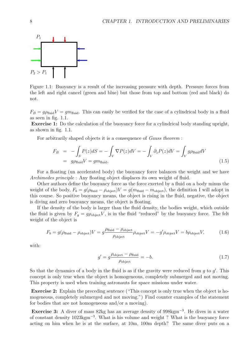
P1
P2 > P1
Figure 1.1: Buoyancy is a result of the increasing pressure with depth. Pressure forces fromthe left and right cancel (green and blue) but those from top and bottom (red and black) donot.
FB = gρfluidV = gmfluid. This can easily be verified for the case of a cylindrical body in a fluidas seen in fig. 1.1.Exercise 1: Do the calculation of the buoyancy force for a cylindrical body standing upright,as shown in fig. 1.1.
For arbitrarily shaped objects it is a consequence of Gauss theorem :
FB = −∫
S
P (z)dS = −∫
V
∇P (z)dV = −∫
V
∂zP (z)dV =
∫
V
gρfluiddV
= gρfluidV = gmfluid, (1.5)
For a floating (un accelerated body) the buoyancy force balances the weight and we haveArchimedes principle : Any floating object displaces its own weight of fluid.
Other authors define the buoyancy force as the force exerted by a fluid on a body minus theweight of the body, Fb = g(ρfluid − ρobject)V = g(mfluid −mobject), the definition I will adopt inthis course. So positive buoyancy means, the object is rising in the fluid, negative, the objectis diving and zero buoyancy means, the object is floating.
If the density of the body is larger than the fluid density, the bodies weight, which outsidethe fluid is given by Fg = gρobjectV , is in the fluid “reduced” by the buoyancy force. The feltweight of the object is
Fb = g(ρfluid − ρobject)V = gρfluid − ρobject
ρobjectρobjectV = −g′ρobjectV = bρobjectV, (1.6)
with:
g′ = gρobject − ρfluid
ρobject= −b. (1.7)
So that the dynamics of a body in the fluid is as if the gravity were reduced from g to g′. Thisconcept is only true when the object is homogeneous, completely submerged and not moving.This property is used when training astronauts for space missions under water.
Exercise 2: Explain the preceding sentence (“This concept is only true when the object is ho-mogeneous, completely submerged and not moving.”) Find counter examples of the statementfor bodies that are not homogeneous and/or a moving).
Exercise 3: A diver of mass 82kg has an average density of 998kgm−3. He dives in a waterof constant density 1023kgm−3. What is his volume and weight ? What is the buoyancy forceacting on him when he is at the surface, at 10m, 100m depth? The same diver puts on a
1.2. BUOYANCY OF AN OBJECT IN HETEROGENEOUS FLUID 9
weight-belt increasing his average density of 1100kgm−3. What is the buoyancy force acting onhim when he is at 10m, 100m depth, at the surface? How much time does it take him to “fall”too a depth of 100m.
Exercise 4: A floating iceberg which is formed of sea water, is melting. How does this changethe sea-level of the worlds ocean.
Exercise 5: A floating iceberg which is formed of fresh water, is melting. How does thischange the sea-level of the worlds ocean.
Exercise 6: A floating iceberg which is formed of sea water and contains a substantial amountof solid rock, is melting. How does this change the sea-level of the worlds ocean.
Exercise 7: (***) The hull of a boat has a parabolic cross-section, it is 50m large and 50mhigh. Consider the stability of the boat as a function of its density (the boat is supposed to behomogeneous).
Exercise 8: Show that in a homogeneous and incompressible fluid the buoyancy of an (in-compressible) object does not depend on depth nor on the orientation of the object in the fluid(Gauss theorem).
1.2 Buoyancy of an object in heterogeneous fluid
We have seen that the buoyancy force acting on an object is given by: Fb = bV ρ when thefluid has varying density the force is also varying in space. The simplest case of a fluid withvariable density is to consider the case where the density variation is a linear function of depth:ρ(z) = ρ0+(∂zρ)(z−z0), where ∂zρ (< 0) is called the vertical density stratification. If an objectof density ρobject is released in a fluid with a density stratification it will settle at an equilibriumdepth at which the fluid density equals its density zeq = z0 +(ρ0 − ρobject)/(∂zρ), that is, whereits buoyancy vanishes. It will approach this equilibrium by performing oscillations. If frictionis neglected the (angular) frequency of these oscillation is given by:
N =√
∂zb, (1.8)
it is called the buoyancy frequency or Brunt-Vaisala frequency . The period of these oscillationsis T = 2π/N (there is a 2π-factor as it is an angular-frequency). Indeed the buoyancy forceper volume is Fb = g(∂zρ)z, where z is the vertical distance from the neutral density level (notethat ∂zρ < 0). Newtons second law reads: ρ∂ttz = g(∂zρ)z which has solutions of the form:z = A sin(Nt) + B cos(Nt), where N is given by eq. (1.8), the constants A and B depend onthe initial conditions (position and velocity).
In the troposphere N ≈ 10−2s−1 leading to oscillations with a period of ≈ 10min.Exercise 9: In the ocean the thermal expansion coefficient is α ≈ 2 10−4K−1. Calculate N foran ocean with a stratification of: (a) 10−4Km−1 (deep ocean), (b) 10−2Km−1, (c) 10−1Km−1
(thermocline).Exercise 10: A diver of mass 82kg has an average density of 1020kgm−3. He dives in a waterof density 1018kgm−3 at the surface and a density gradient of ∂zρ = −2. 10−2kgm−4. What isthe buoyancy force acting on him when he is floating at the surface, at 10m, 100m and 200mdepth? Give the variation of his depth as a function of time when the diver is initially motionless at the surface. Viscous forces will act on the diver while moving vertically in the water.We suppose that the friction can be described by a linear Rayleigh friction Fr = rm∂tz. Givethe variation of his depth as a function of time when the diver is initially motion less at thesurface for the friction values of r = 1, 5. 10−2 and 10−2s−1.
10 CHAPTER 1. INTRODUCTION AND PRELIMINARIES
Exercise 11: In the ocean water-masses are often separated by rather sharp density interfaces.In this exercise we suppose the density interface to be of vanishing thickness. Suppose thatin the upper 50m the temperature of a water mass is 20oC and below it is 10oC, the thermalexpansion coefficient of sea water is α = 2. 10−4K−1. Discuss the motion of an object of densityρ that is released at a depth z0.
1.3 Equation of State and Potential Temperature and
Density
Temperature is measured in degrees Celsius (oC) and temperature differences in Kelvin (K),oceanographers are however slow in adapting to the SI unit Kelvin to measure temperaturedifferences.
The temperature of the world ocean typically ranges from −2oC (−1.87oC freezing point forS = 35 at surface) (freezing temperature of sea water) to 32oC. About 75% of the world oceanvolume has a temperature below 4oC. Before the opening of the Drake Passage 30 million yearsago due to continental drift, the mean temperature of the world ocean was much higher. Thetemperature difference in the equatorial ocean between surface and bottom waters was about7K compared to the present value of 26K. The temperature in the Mediterranean Sea is above12oC even at the bottom and in the Red Sea it is above 20oC.
If one takes a mass of water at the surface and descends it adiabatically (without exchangingheat with the environment) its in situ (Latin for: in position; the temperature you actuallymeasure if you put a thermometer in the position) temperature will increase due to the increaseof pressure. Indeed if you take a horizontal tube that is 5km long and filled with water of salinityS = 35psu and temperature T = 0oC and put the tube to the vertical then the temperature inthe tube will monotonically increase with depth reaching T = 0.40oC at the bottom. To get ridof this temperature increase in measurements oceanographers often use potential temperatureθ (measured in oC) that is the temperature of a the water mass when it is lifted adiabaticallyto the sea surface. It is always preferable to use potential temperature, rather than in situtemperature, as it is a conservative tracer. Differences between temperature and potentialtemperature are small in the ocean < 1.5K, but can be important in the deep ocean wheretemperature differences are small.
In the previous sections we looked at objects of constant density in a fluid of varying density.Things become more involved if the submerged object is itself subject to density changes dueto changes in pressure, temperature or other influences. This is the case for a fluid parcelsubmerged in a fluid. One difficulty is that the density of a fluid parcel is not a quantitythat is conserved with the flow. If a parcel of fluid is displaced vertically in the fluid columnits density changes due to pressure changes. Another difficulty is that density is difficult tomeasure directly for air in the atmosphere or sea water in the ocean. The first step is to obtainthe density of a fluid as a function of a certain number of its properties. Such a relation iscalled an equation of state:
ρ = ρ(S, T, P ) (1.9)
where the density of sea water, chosen here as an example, is a function S,T,P, that is salinity,temperature and pressure, respectively. It can be shown that the density of sea water and airis determined by three independent physical properties. For the case of the atmosphere thedensity is a function of temperature, humidity (water content) and pressure. For an avalanchethe density is mostly determined by temperature and water (snow) content. The density is often
1.4. STATIC STABILITY 11
a non-linear and complicated function of the other fluid properties which is mostly determinedempirically in laboratory experiments and looked up in tables or calculated by functions whichare a best fit to laboratory measurements.
If one takes a mass of water at the ocean surface or a mass of air at high altitude anddescends it adiabatically (without exchanging heat with the environment) its in situ (Latinfor: in position; the density you actually measure if you put a thermometer in the position)density will increase due to the increase of pressure. To get rid of this density increase inmeasurements scientists often use potential density ρθ that is the density of a fluid parcel whenit is moved adiabatically to a reference level (the sea level). It is always preferable to usepotential density, rather than in situ density, as it is a conservative tracer. Differences betweendensity and potential density are unimportant in the laboratory (why?), but can be importantin the atmosphere and the deep ocean.
The same concept applies to temperature of sea water or air in the atmosphere. When a massof fluid is moved adiabatically downward the increase in pressure will increase the temperature(≈ 10K/km for the dry and ≈ 5K/km for the moist atmosphere). The potential temperature θis thus introduced. It is the temperature of the fluid when moved adiabatically to a referencepressure (level). A consequence is that the potential density is given as a function of potentialtemperature. An adiabatic atmosphere is an atmosphere where the potential temperature θ isconstant, an isothermal atmosphere is when (T = const).
Exercise 12: A diver who weighs 82kg has an average density of 1015kgm−3. He dives ina water of density 1018kgm−3 at the surface and a density gradient of ∂zρ = −2. 10−2kgm−4.At the surface he has 6litres of air (perfect gas)in his lounges. What is his density, weight andcompressibility ? What is the buoyancy force acting on him at 0m, 10m, 100m depth? Whathappens if he dives to a depth of 10m and exhales half of the air in his lounges?
Exercise 13: Explain the physics of a “Cartesian diver”.
1.4 Static Stability
A mass of fluid subject to gravitational acceleration is in equilibrium if the gravitational force isbalanced by the pressure force this is called the hydrostatic equilibrium as expressed by eq. (1.4).This shows that for a static fluid the density has to be constant in every horizontal plane, ashorizontal pressure differences create horizontal pressure gradients which can not be balanced bya vertical gravitational force (in rotating flows the Coriolis force can balance horizontal pressuregradients leading to a “geostrophic equilibrium”). If lighter fluid superposes heavier fluid thisequilibrium is stable as restoring forces counter act to departures of this equilibrium. In theinverse case forces destroy the unstable equilibrium and a stable equilibrium will be establishedafter some time, after a redistribution of fluid masses due to (turbulent) fluid motion occurred.This, often violent, vertical exchange of water masses is called convection. (Warning: In olderliterature and in the engineering community the term “convection” is often used for what istoday called “advection”)
Exercise 14: Is an isothermal atmosphere stable?
Exercise 15: Is an atmosphere of constant density stable?
Convection is a process of paramount importance in the ocean and atmosphere as it ex-changes fluid masses in the vertical.
Static stability and static stability parameters are of great importance to scientist to un-derstand convective weather patterns in the atmosphere and circulation patterns in the ocean.
12 CHAPTER 1. INTRODUCTION AND PRELIMINARIES
If the atmosphere is well mixed it has a constant potential temperature and a constantpotential density. In this case the atmosphere is called neutrally stable as no forces (exceptfriction) act to oppose vertical movement and no energy is necessary to exchange or movearound fluid parcels. Considering the stability by adiabatic movement of fluid parcels is calledthe parcel method. The parcel is a hypothetical expandable box that does not allow anytransfer of heat into or out of the box. The stability of the parcel is dependent upon theparcel’s motion after a forced displacement from its original location. A parcel that is forcedback to its original position is considered stable while one that is forced away from its originalposition is unstable. One that is displaced with no force acting on it is considered neutral.An important quantity to investigate the stability is the laps rate Γ = −∂zT , which gives thedecrease of temperature with height. If the potential temperature θ is constant the atmosphereis adiabatic (Γadiabatic ≈ 10K/km) and the atmosphere is neutrally stable, if Γ < Γadiabatic theatmosphere is stable (the temperature decreases less rapidly than for a mixed atmosphere) andunstable if Γ > Γadiabatic.Exercise 16: Further complication arise because Γadiabatic is a function of potential tempera-ture and humidity. What is the meaning of absolute stability, absolute instability, conditionalinstability and potentially unstable.
Exercise 17: What is the layer method of determining stability
1.5 Buoyancy in a fluid of varying density
Gravity is constantly seeking to put fluid in a stably stratified equilibrium. This process is coun-teracted by other phenomena constantly trying to perturb this equilibrium. The competitionbetween this tendencies creates fluid motion.
Buoyancy is the product of density and gravity, the latter shows only minor variationswithin the thin layer of fluid motion at the surface of our planet and can thus be treated asa constant for applications in environmental fluid dynamics. Variations in buoyancy are thusequivalent to density variations.
There are conceptually two ways of changing the buoyancy of a fluid parcel, the first is tochange its properties as for example pressure, temperature, salinity (for water) and humidity(for air) by displacement, fluxes of heat and fluxes of fresh water (rain) evaporation. Anotherway is to mix to masses of fluid of different density. Mixing is not possible for an object in afluid and we will see that mixing plays an important part in the dynamics of buoyancy drivenflows in the environment.
1.6 Boussinesq approximation
Density differences in fluids are usually small and their influence on the inertia of a fluid canoften be neglected. In the ocean potential density variations are mostly smaller than 3/1000and in the atmosphere variations of potential density are typically small in the troposphere.The small density differences are however important when considering the buoyancy of fluidvolumes. At every horizontal level the average buoyancy force is counter acted by a pressureforce due to the presence of horizontal boundaries and only the deviations of buoyancy from thehorizontal mean (the relative buoyancy) is dynamically important. The Boussinesq approxima-tion consists in neglecting density differences in the equations except if they are multiplied byg which is usually much bigger than the vertical accelerations within the fluid. The Boussinesqapproximation is made in the major part of this lecture.
1.7. HEAT TRANSPORT 13
The buoyancy is a convenient quantity when writing down the Bousinesq equations wherethe acceleration term per fluid volume is usually divided by a reference density. When thebuoyancy force per fluid volume is usually divided by a reference density it is buoyancy, so thatthe equations read:
d
dtw = ...+ b, (1.10)
so the main motivation to introduce buoyancy is to make equations look easier.When the fluid is homogeneous, of constant density, the gravity force is often omitted in the
equations and calculations. This is possible as there is a the hydrostatic pressure gradient thatbalances the gravitational force ∂zPhydrostat = −gρ0. The real preassure can than be written asP = Phydrostat+P
′. Replacing P by P ′ and omitting gravity in the equations leads to the samesolutions. If there are density differences in the fluid this is no-longer possible.
1.7 Heat Transport
Heat (thermal energy) can be transported by three different mechanisms.Radiation: Thermal radiation is generated by the thermal motion of charged particles in
matter. Every object is radiating heat at a rate which is proportional to the fourth power ofits temperature P = σ ·A ·T 4 where σ = 5.670373(21) 10−8W m−2 K−4 is the StefanBoltzmannconstant, A the surface area of the object and T its temperature measured in Kelvin.
Molecular transport: is the transport of heat due to molecular motion it is given byits thermal diffusivity κ, which depends on the substance and its physical parameters as forexample temperature, pressure, composition κair ≈ 2. 10−5m2s−1, κair ≈ 1. 10−7m2s−1. It isequivalent to thermal conduction in solids.
Convection: is the advective transport of heat by fluid motion.Exercise 18: A spherical air parcel of radius of 1m has a temperature anomaly depending onthe radius r of T = 1K(1− r/(1m)) + 20oC in a surrounding fluid of 20oC and is moving witha speed of 1ms−1. Compare the loss of heat due to radiation, diffusion and the convection dueto the motion of the parcel.
14 CHAPTER 1. INTRODUCTION AND PRELIMINARIES
Chapter 2
Hydraulics
In this chapter we will suppose that the the fluid is incompressible, that is, density does notdepend on pressure. If the density of a fluid is constant the conservation of mass leads to theconservation of volume, that is, the flow is divergence free. We furthermore suppose that theflow is time independent.
2.1 Bernoulli Equation
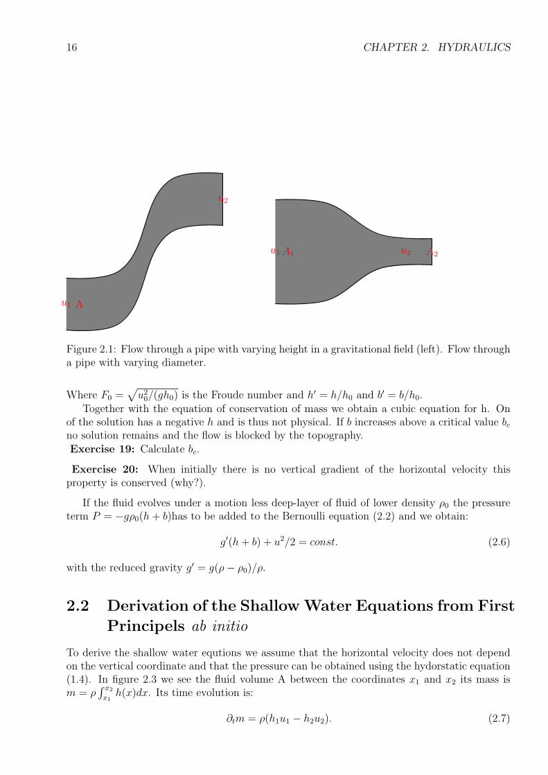
In this section we will consider a stationary (=time-independent) flow in tubes of varying sectionin a gravitational field. We neglect friction in the flow due to viscosity. The conservation ofvolume states that the transport of volume at a time interval ∆t through every cross sectionis equal along the flow (∆t u1A1 = ∆t u2A2). This leads to: uA = const along the tube. Thismeans that in parts of the tube with a smaller cross-section the fluid has to move faster. Letslook at a fluid volume between cross-section 1 and 2. If a fluid particle has moved ∆l1 atlocation 1 a particle at location 2 has moved ∆l2. The change of kinetic energy of the fluidvolume is: ∆Ekin = (ρ/2)(∆l2A2u
22 −∆l1A1u
21). The force that accelerates the fluid is due to
the pressure difference at P2 and P1. The difference of work done at location 2 and 1 by thepressure is: ∆W = P1A1∆l1−P2A2∆l2. Conservation of energy gives: P1−P2 = (ρ/2)(u22−u21)or P1+(ρ/2)u21 = P2+(ρ/2)u22. The same reasoning can be made for the work done by pressureagainst gravity and we obtain: P1 + gρh1 + (ρ/2)u21 = P2 + gρh2 + (ρ/2)u22 or more generally:
P + ρgh+ (ρ/2)u2 = const. (2.1)
along any stream-line, which is the Bernoulli equation.If we consider a flow with a free surface than the Bernoulli equation can be applied to the
free surface, which is a streamline with no pressure, and we get
g(h+ b) + u2/2 = const. (2.2)
We now consider the flow over a topographic obstacle as shown in fig. 2.2. Far from theobstacle we have the velocity u0 and the layer thickness h0. Bernoulli equation teaches us that:g(h(x) + b(x)) + u(x)2/2 = gh0 + u20/2 = const. for all x. This leads to:
g(h+ b)
u20+
u2
2u20=gh0u20
+1
2(2.3)
gh0u20
(h′ + b′) +1
2h′2=gh0u20
+1
2(2.4)
h′ +F 20
2h′2= 1− b′ +
F 20
2(2.5)
15
16 CHAPTER 2. HYDRAULICS
Au1
u2
A1u1 A2u2
Figure 2.1: Flow through a pipe with varying height in a gravitational field (left). Flow througha pipe with varying diameter.
Where F0 =√
u20/(gh0) is the Froude number and h′ = h/h0 and b′ = b/h0.Together with the equation of conservation of mass we obtain a cubic equation for h. On
of the solution has a negative h and is thus not physical. If b increases above a critical value bcno solution remains and the flow is blocked by the topography.Exercise 19: Calculate bc.
Exercise 20: When initially there is no vertical gradient of the horizontal velocity thisproperty is conserved (why?).
If the fluid evolves under a motion less deep-layer of fluid of lower density ρ0 the pressureterm P = −gρ0(h+ b)has to be added to the Bernoulli equation (2.2) and we obtain:
g′(h+ b) + u2/2 = const. (2.6)
with the reduced gravity g′ = g(ρ− ρ0)/ρ.
2.2 Derivation of the ShallowWater Equations from First
Principels ab initio
To derive the shallow water equtions we assume that the horizontal velocity does not dependon the vertical coordinate and that the pressure can be obtained using the hydorstatic equation(1.4). In figure 2.3 we see the fluid volume A between the coordinates x1 and x2 its mass ism = ρ
∫ x2
x1
h(x)dx. Its time evolution is:
∂tm = ρ(h1u1 − h2u2). (2.7)
2.3. FROM THE NAVIER-STOKES TO THE SHALLOW WATER EQUATIONS 17
subcriticalu1, h1 u2, h2
supercriticalu1, h1 u2, h2
subcritical
supercriticalu1, h1 u2, h2
Figure 2.2: Shallow water flow over an obstacle
If ∆x = x2 − x1 is very small we see that to first order m = ρh∆x, where h is a value of theheight within the interval [x1, x2]. Introducing this in eq. (2.7) and supposing that the variablesare sufficiently smooth, gives:
∂th+ ∂x(uh) = 0. (2.8)
The inertia of the volume A is M = ρ∫ x2
x1
u(x)h(x)dx. Its time evolution is:
∂tM = ρ(
h1u21 − h2u
22 +
g
2(h21 − h22)
)
. (2.9)
The last term is the pressure force acting at x1 and x2, it is calculated using hydrostaticity.The above equation is Newtons second law applied to the are A. If ∆x is very small we see thatto first order M = ρhu∆x. In troducing this in eq. (2.9) gives:
∂tuh+ ∂x(u2h) + gh∂xh = 0. (2.10)
Exercise 21: Show that the system given by eqs. (2.8) and (2.10) is equivalent to eq. (2.8)and ∂tu+ u∂xu+ g∂xh = 0.
2.3 From the Navier-Stokes to the Shallow Water Equa-
tions
The dynamics of and incompressible fluid is described by the Navier-Stokes equations:
∂tu+ u∂xu+ v∂yu+ w∂zu+1ρ0∂xP = ν∇2u (2.11)
∂tv+ u∂xv + v∂yv + w∂zv +1ρ0∂yP = ν∇2v (2.12)
∂tw+ u∂xw + v∂yw + w∂zw + 1ρ0∂zP = −g ρ
ρ0+ ν∇2w (2.13)
∂xu+ ∂yv + ∂zw = 0 (2.14)
+ boundary conditions
where u is the zonal, v the meridional and w the vertical (positive upward even in oceanography)velocity component, P the pressure, ρ density, ρ0 the average density, ν viscosity of sea water,g gravity, and ∇2 = ∂xx + ∂yy + ∂zz is the Laplace operator.
18 CHAPTER 2. HYDRAULICS
A
x1 x2
u1, h1
u2, h2
Figure 2.3: Shallow water layer
The equation of a scalar transported by a fluid is:
∂tT+ u∂xT + v∂yT + w∂zT = κT∇2T (2.15)
+boundary conditions (2.16)
∂tS+ u∂xS + v∂yS + w∂zS = κS∇2S (2.17)
+boundary conditions ,
where T is temperature, S is salinity and κT , κS are the diffusivities of temperature and salinity.The state equation:
ρ = ρ(S, T, P ) (2.18)
allows to obtain the density from salinity, temperature and pressure.The above equations describe the motion of the ocean to a very high degree of accuracy,
but they are much too complicated to work with, even today’s and tomorrows numerical oceanmodels are and will be based on more or less simplified versions of the above equations.
These equations are too complicated because:
• Large range of scales; from millimetre to thousands of kilometres
2.3. FROM THE NAVIER-STOKES TO THE SHALLOW WATER EQUATIONS 19
A large part of physical oceanography is in effect dedicated to finding simplifications of theabove equations. In this endeavour it is important to find a balance between simplicity andaccuracy.
How can we simplify these equations? Two important observations:
• The ocean is very very flat: typical depth (H=4km) typical horizontal scale (L=10 000km)
• Sea water has only small density differences ∆ρ/ρ ≈ 3 · 10−3
X
Z
H
η
Figure 2.4: Shallow water configuration
Using this we will try to model the ocean as a shallow homogeneous layer of fluid, and seehow our results compare to observations.
Using the shallowness, equation (2.14) suggests that w/H is of the same order as uh/L,where uh =
√u2 + v2 is the horizontal speed, leading to w ≈ (Huh)/L and thus w ≪ uh. So
that equation (2.13) reduces to ∂zP = −gρ which is called the hydrostatic approximation asthe vertical pressure gradient is now independent of the velocity in the fluid.
Using the homogeneity ∆ρ = 0 further suggest that:
∂xzP = ∂yzP = 0. (2.19)
If we derive equations (2.11) and (2.12) with respect to the vertical direction we can see that if∂zu = ∂zv = 0 at some time this property will be conserved such that u and v do not vary withdepth (We have neglected bottom friction). Putting all this together we obtain the followingequations:
∂tu+ u∂xu+ v∂yu+1ρ∂xP = ν∇2u (2.20)
∂tv+ u∂xv + v∂yv +1ρ∂yP = ν∇2v (2.21)
∂xu+ ∂yv + ∂zw = 0 (2.22)
with ∂zu = ∂zv = ∂zzw = 0 (2.23)
+ boundary conditions
What are those boundary conditions? Well on the ocean floor, which is supposed to vary onlyvery slowly with the horizontal directions, the vertical velocity vanishes w = 0 and it varieslinearly in the fluid interior (see eq. 2.23). The ocean has what we call a free surface with aheight variation denoted by η. The movement of a fluid particle on the surface is governed by:
dHdtη = w(η) (2.24)
20 CHAPTER 2. HYDRAULICS
where dHdt
= ∂t + u∂x + v∂y is the horizontal Lagrangian derivation. We obtain:
Using the hydrostatic approximation, the pressure at a depth d from the unperturbed freesurface is given by: P = gρ(η + d), and the horizontal pressure gradient is related to thehorizontal gradient of the free surface by:
∂xP = gρ∂xη and ∂yP = gρ∂yη (2.27)
Some algebra now leads us to the shallow water equations (sweq):
∂tu+ u∂xu+ v∂yu+ g∂xη = ν∇2u (2.28)
∂tv+ u∂xv + v∂yv + g∂yη = ν∇2v (2.29)
∂tη+ ∂x [(H + η)u] + ∂y [(H + η)v] = 0 (2.30)
+boundary conditions .
All variables appearing in equations (2.28), (2.29) and (2.30) are independent of z!
2.4 The Linearised One Dimensional ShallowWater Equa-
tion
We will now push the simplifications even further, actually to its non-trivial limit, by consideringthe linearised one dimensional shallow water equations. If we suppose the dynamics to beindependent of y and if we further suppose v = 0 and that H is constant, the shallow waterequations can be written as:
∂tu+ u∂xu+ g∂xη = ν∇2u (2.31)
∂tη+ ∂x [(H + η)u] = 0 (2.32)
+ boundary conditions.
if we further suppose that u2 ≪ gη that the viscosity ν ≪ gηL/u and η ≪ H then:
∂tu+ g∂xη = 0 (2.33)
∂tη +H∂xu = 0 (2.34)
+boundary conditions,
which we combine to:
∂ttη = gH∂xxη (2.35)
+boundary conditions.
This is a one dimensional linear non-dispersive wave equation. The general solution is givenby:
η(x, t) = η−0 (ct− x) + η+0 (ct+ x) (2.36)
u(x, t) =c
H(η−0 (ct− x)− η+0 (ct+ x)), (2.37)
2.5. REDUCED GRAVITY 21
where η−0 and η+0 are arbitrary functions of space only. The speed of the waves is given byc =
√gH and perturbations travel with speed in the positive or negative x direction. Note
that c is the speed of the wave not of the fluid!Rem.: If we choose η−0 (x) = η+0 (−x) then initially the perturbation has zero fluid speed,
and is such only a perturbation of the sea surface! What happens next?An application of such equation are Tsunamis if we take: g = 10m/s2, H = 4km and
η0 = 1m, we have a wave speed of c = 200m/s= 720km/h and a fluid speed u0 = 0.05m/s.What happens when H decreases? Why do wave crests arrive parallel to the beach? Why dowaves break?
You see this simplest form of a fluid dynamic equation can be understood completely. Ithelps us to understand a variety of natural phenomena.
Exercise 22: Does the linearised one dimensional shallow water equation conserve energy?
Exercise 23: Is it justified to neglect the nonlinear term in eq. (2.31) for the case of aTsunami?
2.5 Reduced Gravity
Suppose that the layer of fluid (fluid 1) is lying on a denser layer of fluid (fluid 2) that isinfinitely deep. H2 → ∞ ⇒ c2 → ∞, that is perturbations travel with infinite speed. Thisimplies that the lower fluid is always in equilibrium ∂xP = ∂yP = 0. The lower fluid layer ispassive, does not act on the upper fluid but adapts to its dynamics, so that η1 =
ρ1−ρ2ρ1
η2. If weset η = η1 − η2 then η = ρ2
ρ2−ρ1η1 and the dynamics is described by the same sweqs. 2.28, 2.29
and 2.30 with gravity g replaced by the reduced gravity g′ = ρ2−ρ1ρ2
g (“sw on the moon”).
Example: g′ = 3 · 10−3g, H = 300m, η0 = .3m we get a wave speed c =√g′H = 3m/s and
a fluid speed of u = 1m/s.
X
Z
ρ1
ρ2
∂xP1 = gρ1∂xη1
∂xP2 = gρ1∂xη1 + g(ρ2 − ρ1)∂xη2 = 0
η1
η2
Figure 2.5: Reduced gravity shallow water configuration
Comment 1: When replacing gη by g′η it seems, that we are changing the momentumequations, but in fact the thickness equation is changed, as we are in the same time replacing
22 CHAPTER 2. HYDRAULICS
the deviation of the free surface η (which is also the deviation of the layer thickness in not-reduced-gravity case) by the deviation of the layer thickness η , which is (ρ2 − ρ1)/ρ2 timesthe surface elevation in the reduced gravity case. This means also that every property whichis derived only from the momentum equations not using the thickness equation is independentof the reduced gravity.
Comment 2: Fig. 2.5 demonstrates, that the layer thickness can be measured in twoways, by the deviation at the surface (η1) or by density structure in the deep ocean (η2). Forocean dynamics the surface deviation for important dynamical features, measuring hundredsof kilometres in the horizontal, is usually less than 1 m whereas variations of (η2) are usuallyseveral hundreds of meters. Historically the measurement of the density structure of the oceanto obtain η2 are the major source of information about large scale ocean dynamics. Nowadayssatellites measure the surface elevation of the ocean (altimetry) at a spatial and temporaldensity unknown before and are today our major source of information.
2.6 Bernoulli Revisited
Lets take a second look at the 1D Bernoulli equation which can now be derived from thestationary and in-viscid shallow water equations:
u∂xu+ g∂xη = 0 ; (∂xu2)/2 + g∂xη = 0 ; (u2)/2 + g(h+ b) = B = const. (2.38)
∂x [hu] = 0 ; hu = Q = const, (2.39)
where h = H + η − b, thickness of the fluid layer. We combine these two equations to:
Q2
2h2+ g(h+ b) = B ; P (h) = gh3 + (gb−B)h2 +
Q2
2= 0 (2.40)
this cubic polynome has one or three real solutions. The local extrema of the cubic are at
3gh2 + 2(gb−B)h = 0 ; h1 = 0 and h2 =2(B − gb)
3g(2.41)
As P (h1) > 0, one solution for P (h) = 0 is negative, which is not physical. At h2 we getFr = 1:
h2 =2(B − gb)
3g=u22 + 2gh2
3g; 3gh2 = u22 + 2gh2 ; Fr2 =
u2
gh2= 1 (2.42)
There is no real positive solution if gh32 + (gb−B)h22 +Q2/2 > 0, one solution for equality andtwo solutions (a sub-critical and a super-critical one), when the inequality is inverted. If forb = 0 we have two solutions and B = B0 then the maximum value for b to have at least onesolution is when:
B0 − gb =3gh22
; b =2B0 − 3gh2
2g. (2.43)
For higher topographies the flow is blocked.
2.6.1 Hydraulic Jump
When a super critical flow is slowed down by an obstacle or a change in the slope, it can suddenlybecome sub-critical. This phenomena is called a hydraulic jump. They can be observed in rivers,
2.6. BERNOULLI REVISITED 23
h
B − gb
h2 = 2(B − gb)/3g
3gh2/2
gh
√
2(B − gb)/Q
conjugateddepths
alternativedepths
Figure 2.6: The two positive solutions of the thickness h as a function of B − gb are given.The asymptotics for long and small h are also shown. The green arrow indicates the hydraulicjump.
24 CHAPTER 2. HYDRAULICS
especially after a flow has passed from sub to super-critical over a dam and then recovers tosub-critical afterwards. It has many applications in this context (reducing energy, mixing,sediment transport, oxygenizing, ...). In the atmosphere and ocean hydraulic jumps also occurat many locations. They are important in fluid dynamics as they lead to very violent mixingof the fluid, because the energy lost to the mean flow is put into small scale turbulent motion.The hydraulic jump is an example of a very localised mixing process.
This phenomena can NOT be described by the shallow water equations as the horizontalvelocity is no longer independent of the vertical direction. Energy is not conserved but destroyedby the jump. The quantities conserved are the mass and the momentum. Please note that inthe shallow water context the conservation of momentum and mass leads to a conservation ofenergy, if no forces (by the topography) are applied. Note also that if over a topography theflow tansits from sub- to super-critical momentum is not conserved as the topography exerts aforce, but energy is conserved as, in the absence of friction, there are no dissipative processesacting on the flow. When both momentum and energy are conserved over a flat bottom flow,neither velocity nor layer thickness can change. Before the jump we have (u1, h1) and after thejump (u2, h2). The Bernoulli function is no longer conserved. The jump provides a dissipativeprocess. Transport
u1h1 = u2h2 (2.44)
is conserved (the jump does not make water disappear) and the momentum budget
h1u21 + gh21/2 = h2u
22 + gh22/2 (2.45)
(momentum per density is uhl and the momentum per density passing at the point 1 per timeis h1u
21, the depth-averaged pressure per density at point 1 is gh1/2 and force difference acting
at point 1 and point 2 is gh21/2− gh22/2. Note that in a hydraulic jump the (turbulent) surfacedoes not excert an acceleration force on the water colomn as the flow is not hydrostatic. Theabove leads to (Belanger equation):
u1u2
=h2h1
= (Fr1Fr2
)2/3 =
√
1 + 8Fr21 − 1
2. (2.46)
First equality is an immediate consequence of conservation of transport as is the second.
Exercise 24: Show the third equality
For the third equality
h1u21 + gh21/2 = h2u
22 + gh22/2 ; 2u21(h1 −
h21h2
) + g(h21 − h22) = 0
; 2Fr21(1−h1h2
) + (1− h22h21
) = 0 ; 2Fr21 =h2h1
(1− h1
h2
)(1 + h2
h1
)
(1− h1
h2
)
;h2h1
(h2h1
+ 1)− 2Fr1 = 0 (2.47)
The change in B is:
∆B = g(h2 − h1)
3
4h2h1. (2.48)
Exercise 25: Calculate ∆B
Hydraulic jumps are used in engineering applications to dissipate energy or to entrain airinto the water. A sub-critical flow can not suddenly become super-critical because this wouldrequire a sudden increase of energy.
2.7. BERNOULLI IN 2D 25
high pressure low pressure
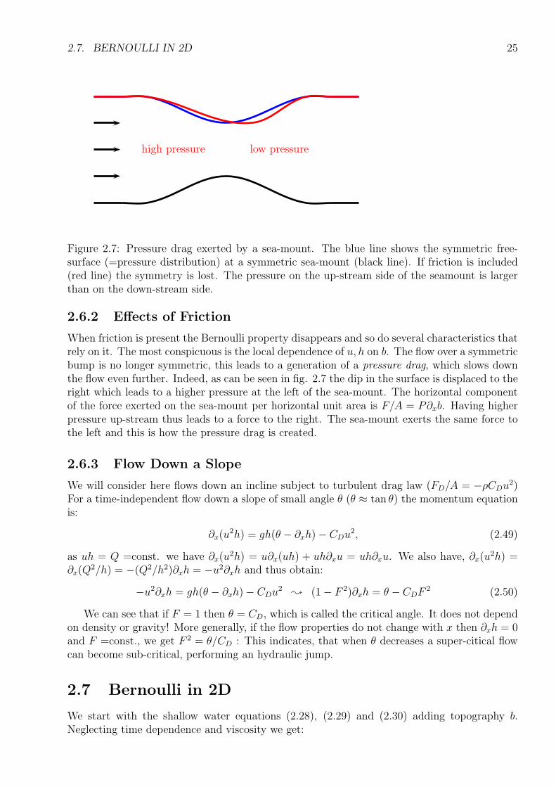
Figure 2.7: Pressure drag exerted by a sea-mount. The blue line shows the symmetric free-surface (=pressure distribution) at a symmetric sea-mount (black line). If friction is included(red line) the symmetry is lost. The pressure on the up-stream side of the seamount is largerthan on the down-stream side.
2.6.2 Effects of Friction
When friction is present the Bernoulli property disappears and so do several characteristics thatrely on it. The most conspicuous is the local dependence of u, h on b. The flow over a symmetricbump is no longer symmetric, this leads to a generation of a pressure drag, which slows downthe flow even further. Indeed, as can be seen in fig. 2.7 the dip in the surface is displaced to theright which leads to a higher pressure at the left of the sea-mount. The horizontal componentof the force exerted on the sea-mount per horizontal unit area is F/A = P∂xb. Having higherpressure up-stream thus leads to a force to the right. The sea-mount exerts the same force tothe left and this is how the pressure drag is created.
2.6.3 Flow Down a Slope
We will consider here flows down an incline subject to turbulent drag law (FD/A = −ρCDu2)
For a time-independent flow down a slope of small angle θ (θ ≈ tan θ) the momentum equationis:
∂x(u2h) = gh(θ − ∂xh)− CDu
2, (2.49)
as uh = Q =const. we have ∂x(u2h) = u∂x(uh) + uh∂xu = uh∂xu. We also have, ∂x(u
2h) =∂x(Q
2/h) = −(Q2/h2)∂xh = −u2∂xh and thus obtain:
−u2∂xh = gh(θ − ∂xh)− CDu2
; (1− F 2)∂xh = θ − CDF2 (2.50)
We can see that if F = 1 then θ = CD, which is called the critical angle. It does not dependon density or gravity! More generally, if the flow properties do not change with x then ∂xh = 0and F =const., we get F 2 = θ/CD : This indicates, that when θ decreases a super-citical flowcan become sub-critical, performing an hydraulic jump.
2.7 Bernoulli in 2D
We start with the shallow water equations (2.28), (2.29) and (2.30) adding topography b.Neglecting time dependence and viscosity we get:
26 CHAPTER 2. HYDRAULICS
u∂xu+ v∂yu+ g∂xη = 0 (2.51)
u∂xv + u∂xv + g∂yη = 0 (2.52)
∂x [(H + η − b)u] + ∂y [(H + η − b)v] = 0, (2.53)
note that (H + η) = h+ b. If we define the Bernoulli function as:
B = g(H + η) +u2 + v2
2(2.54)
we obtain using eqs. (2.51), (2.52) and (2.53) that
u∂xB + v∂yB = 0 (2.55)
which states that the Bernoulli function is conserved along stream lines in a 2D stationarynon-viscous shallow water flow.Exercise 26: Show that the Bernoulli function is conserved along stream lines in a 2Dstationary non-viscous shallow water flow.
An interesting feature is that the solutions of (u, η) depend locally on b, that is if you knowb at a location in 2D space and the Bernoulli constant and the transport along a stream lineyou can calculate u and η (well you have the choice between the sub and the super criticalsolution) and you do not have to care what happens at other locations. This nice property islost when friction is considered.
Chapter 3
Vector Fields
3.1 Two Dimensional Flow
We have seen in the previous sections, that the dynamics of a shallow fluid layer can bedescribed by the two components of the velocity vector (u(x, y, t), v(x, y, t)) and the surfaceelevation η(x, y, t) (these are called the dynamic variables). The vertical velocity w(x, y, t), isin this case, determined by these 3 variables (it is called a diagnostic variable). . The verticalvelocities in a shallow fluid layer are usually smaller than their horizontal counterparts and wehave to a good approximation a two dimensional flow field.
The dynamics of a fluid is described by scalar (density, pressure) and vector quantities(velocity). These quantities can be used to construct other scalar quantities (tensors, of orderzero) vectors (tensors, of order one) and higher order tensors. Higher order tensors can than becontracted to form lower order tensors. An example is the velocity tensor (first order) whichcan be used to calculate the speed (its length), it is a tensor of order one. The most useful scalarquantities are those which do not change when measured in different coordinate systems, whichmight be translated by a given distance or rotated by a fixed angle. Such quantities are calledwell defined . For example it is more reasonable to consider the length of the velocity vector(the speed, well defined) rather than the first component of the velocity vector (ill defined),which changes when the coordinate system is rotated. The length of the velocity vector is usedto calculate the kinetic energy. The most prominent second order tensor is the strain tensor,considering the linear deformation of a fluid volume. In two dimension it is:
(∇ut)t =
(
∂xu ∂yu∂xv ∂yv
)
(3.1)
if a coordinate system e′ is rotated by an angle α with respect to the original coordinate systeme the components in the new system are given by:
(
u′
v′
)
=
(
cosα sinα− sinα cosα
)(
uv
)
= Au (3.2)
and u = Atu′. Note that At = A−1.For a scalar field (as for example temperature) we can express in the two coordinate systems:
f ′(x′, v′) = f(x(x′, v′), y(x′, v′)) we have:
∂x′f ′ =∂f ′
∂x′=∂x
∂x′∂f
∂x+∂y
∂x′∂f
∂y(3.3)
its gradient transforms as:
(∂x′f ′, ∂y′f′) = (∂xf, ∂yf)
(
cosα − sinαsinα cosα
)
= (∇f)At (3.4)
27
28 CHAPTER 3. VECTOR FIELDS
and we can write by just adding a second line with a function g (say salinity)
(
∂x′f ′ ∂y′f′
∂x′g′ ∂y′g′
)
=
(
∂xf ∂yf∂xg ∂yg
)(
cosα sinα− sinα cosα
)
= (∇(
fg
)
)At (3.5)
Now u, v are not scalar functions as are g, f but components of a vector so we have to rotatethem from the prime system. And we obtain for the transformation of the strain tensor
where s = sinα and c = cosα. The well defined scalar quantities that depend linearly onthe strain tensor are the trace of the tensor d = ∂xu + ∂yv and the skew-symmetric part ofthe tensor, which gives the vorticity ζ = ∂xv − ∂yu. this can be easily verified looking at eq.(3.6). A well defined quadratic quantity is the determinant of the tensor D = ∂xu∂yv−∂yu∂xv.Other well defined quadratic quantities are the square of vorticity which is called enstrophy,the square of all components of the strain matrices H = d2+ζ2+2D or the square of the strainrate s2 = d2 + ζ2 − 2D, the Okubo-Weiss parameter OW = ζ2 − s2. they are all dependenton the trace, vorticity and determinant. You can construct your own well-defined quantity andbecome famous!
Exercise 27: Show that the vorticity is well defined.
Exercise 28: Show that every well defined quantity which is a linear combination of thecomponents of the strain tensor, is a linear combination of the divergence and the vorticity.
If a variable does not depend on time it is called stationary. The trajectory of a smallparticle transported by a fluid is always tangent to the velocity vector and its speed is givenby the magnitude of the velocity vector. In a stationary flow its path is called a stream line. Ifthe flow has a vanishing divergence it can be described by a stream function Ψ with v = ∂xΨand u = −∂yΨ. If the flow has a vanishing vorticity it can be described by a potential Θ withu = ∂xΘ and v = ∂yΘ. Any vector field in 2D can be written as u = ∂xΘ−∂yΨ, v = ∂yΘ+∂xΨ,this is called the Helmholtz decomposition.
Exercise 29: Show that every flow that is described by a stream function has zero divergence.
Exercise 30: Show that every flow that is described by a potential has zero vorticity.
Exercise 31: Express the vorticity in terms of the stream function.
Exercise 32: Express the divergence in terms of the potential.
Exercise 33: Which velocity fields have zero divergence and zero vorticity?
Exercise 34: draw the velocity vectors and streamlines and calculate vorticity and divergence.Draw the a stream function where ever possible:
(
uv
)
=
(
−x−y
)
;
(
y0
)
;
(
−yx
)
;
(
−xy
)
;1
x2 + y2
(
−yx
)
;
(
cos ysin x
)
. (3.7)
3.2. THREE DIMENSIONAL FLOW 29
3.2 Three Dimensional Flow
Conceptually there is not much different when going from two to three dimensions. divergenceis: d = ∇ · u = ∂xu+ ∂yv + ∂zw. vorticity is no longer a scalar but becomes a vector:
ζ = ∇× u =
ζ1ζ2ζ3
=
∂yw − ∂zv∂zu− ∂xw∂xv − ∂yu
. (3.8)
30 CHAPTER 3. VECTOR FIELDS
Chapter 4
Buoyancy Driven Flows
4.1 Molecular Transport
The molecular thermal diffusivity of sea water is κ ≈ 10−7m2s−1. The diffusion equation in thevertical is given by,
∂tT = ∂z(κ∂zT ). (4.1)
We further suppose that there is a periodic heat flux of magnitude Q at the surface (boundarycondition), that is:
∂zT |z=0 =Q
cpρκcos(2πt/τ + π/4), (4.2)
limz→−∞
∂zT = 0. (4.3)
The linear equation (4.1) with the boundary conditions (4.3) has the solution:
T (z, t) = TAez/L cos(2πt/τ + z/L), (4.4)
with:
TA =Q
cpρ
√
τ
2πκand L =
√
τκ
π. (4.5)
Where Q ≈ 200Wm−2, cp = 4000JK−1kg−1, ρ = 1000kgm−3 if we take τ to be one day we get:TA ≈ 20K and L = 5.2cm, this means that the surface temperature in the ocean varies by 40Kin one day and the heat only penetrates a few centimetres. If τ is one year, considering theseasonal cycle, TA ≈ 400K and L ≈ 1m. This means that the surface temperature in the oceanvaries by 800K in one year and the heat only penetrates about one meter. This does not at allcorrespond to observation!
Exercise 35: Derive eqs. (4.4) and (4.5).
When using the molecular viscosity, ν we can also calculate the thickness of the Ekmanlayer δ =
√
2ν/f which is found to be a few centimetres. The observed thickness of the Ekmanlayer in the ocean is however over 100 times larger.
This shows that molecular diffusion can not explain the vertical heat transport, and molec-ular viscosity can not explain the vertical transport of momentum! But what else can?
31
32 CHAPTER 4. BUOYANCY DRIVEN FLOWS
4.2 Turbulent Transport
In the early 20th century fluid dynamicists as L. Prandtl suggested that small scale turbulentmotion mixes scalars and momentum very much like the molecular motion does, only thatthe turbulent mixing coefficients are many orders of magnitude larger than their molecularcounterparts. This is actually something that can easily be verified by gently poring a littlemilk into a mug of coffee. Without stirring the coffee will be cold before the milk has spreadevenly in the mug, with a little stirring the coffee and milk are mixed in less than a second.
In this section we like to have a quantitative look at the concept of eddy diffusivity in a verysimplified frame work that nevertheless contains all the important pieces. The starting point ofour investigation is the transport equation of a scalar (2.15). We start by considering the twodimensional motion in the x−z-plane. Motion and dependence in the y direction are neglectedonly to simplify the algebra, and do not lead to important changes. We further suppose thatthe large scale scalar field depends only on the z-direction and that the large-scale flow in thez direction vanishes. The x and z component of the motion is given by u and w, respectively.
(
uw
)
=
(
U(z) + u′
w′
)
and s = S(z) + s′ (4.6)
with U(z) = 〈u〉x, W (z) = 〈w〉x and S(z) = 〈s〉x.The 〈.〉x operator denotes the average over a horizontal slice:
A(y) = 〈a(x, z)〉x =1
L
∫
L
a(x, z)dx (4.7)
In the sequel we will use the following rules:
〈λ(z)a〉x = λ(z)〈a〉x (4.8)
〈∂za〉x = ∂z〈a〉x (4.9)
and
〈∂xa(x, z)〉x =1
x2 − x1
∫ x2
x1
∂xa(x, z)dx =a(x2, z)− a(x1, z)
x2 − x1, (4.10)
which vanishes if a(x, z) is bounded and we take the limit of the averaging interval L = (x2−x1) → ∞. But of course:
〈ab〉x 6= 〈a〉x〈b〉x. (4.11)
If we suppose u′ = w′ = 0, that is no turbulence, the transport equation (see eq. (2.15)becomes:
∂tS = κ∂zzS. (4.12)
If we allow for small scale turbulent motion we get:
If we now compare eqs. (4.12) and (4.16) we see that the small scale turbulent motion addsone term to the large scale equations. The value of this term depends on the small scaleturbulence and the large scale flow and is usually unknown. There are now different ways toparametrise this term, that is, express it by means of the large scale flow. The problem offinding a parametrisation is called closure problem.
None of the parametrisations employed today is rigorously derived from the underlyingNavier-Stokes equations, they all involve some “hand-waving.” We will here only discuss thesimplest closure, the so called K-closure (also called Boussinesq assumption).
S
S(z)
s′ < 0w′ > 0
s′ > 0w′ < 0
Figure 4.1: K-closure
The K-closure assumes the turbulent flux term to be proportional to the large-scale gradientof S:
〈w′s′〉x = −κ′eddy∂zS (4.17)
where −κ′eddy is the proportionality coefficient. Looking at fig. 4.1 this choice seems reasonable:firstly the coefficient should be negative as upward moving fluid transport a fluid parcel thatoriginates from an area with a lower average S value to an area with a higher average S , suchthat s′ is likely to be negative. The reverse is true for downward transport. Such that 〈w′s′〉x islikely to be negative. Secondly, a higher gradient is likely to increase |s′| and thus also −〈w′s′〉x.
Using the K-closure we obtain:
∂tS = (κ+ κ′eddy)∂zzS, (4.18)
which is identical to eq. (4.12) except for the increased effective diffusivity κeddy = κ + κ′eddycalled the eddy diffusivity.
Exercise 36: Perform the calculations without neglecting the motion and dependence in they-direction.
34 CHAPTER 4. BUOYANCY DRIVEN FLOWS
4.3 Rayleigh-Benard Convection
The conceptually simplest convective situation is when we have two horizontal plates whichare separated by a distance d. The lower one is heated and the upper one cooled. For smalltemperature differences, cooling rates, the heat transport is done by molecular diffusion ata rate −κ∂zT = κ(Thot − Tcold)/d (minus sign because the flux is down gradient). Whenthe temperature difference increases above a certain threshold fluid motion sets in leading to a“turbulent” transport of heat which ads to the molecular transport. Averaged over a horizontalplane we obtain for the tempreature transport H(z) = 〈wT − κ∂zT 〉x,y. In a statisticallystationary state we can also average over time and the heat transport H becomes independentof z. The turbulent transport is most efficient far from the plates, where the friction of theplates transmitted by viscosity of the fluid is less felt, and w has large values. Please note,that in an incompressible fluid the average vertical velocity is vanishing 〈w〉x,y = 0 and theheat transport is well defined (independent on whether temperature is measured in Celsius orKelvin). In the vicinity of the plates the heat transport is still governed by molecular motionand thus less efficient than in the turbulent interior. This leads to strong temperature gradientsat the plates showing that the overall heat transport in the turbulent case is determined by theboundary layer dynamics (see fig. 4.2).
The external parameters of the system are: diffusivity κ, viscosity ν, distance between theplates d, temperature difference between the plates Thot − Tcold, gravity g and the thermalexpansion coefficient α of the fluid. The last three are combined to form a buoyancy differenceb = gα(Thot − Tcold). Two non dimensional parameters can be formed, the Prandtl numberPr = ν/κ and the Rayleigh number:
Ra =bd3
νκ=gα(Thot − Tcold)d
3
νκ, (4.19)
it is the ratio of two time scales squared t2molec/t2buoyancy. Where tmolec =
√
d4/νκ is the character-
istic time scale of the stabilising action of molecular viscosity and diffusion and tbuoyancy =√
d/bis the characteristic time scale of the destabilising buoyancy gradient. For small Rayleigh num-bers molecular exchange coefficients lead to stability for large Rayleigh numbers the buoyancygradient wins. In problems where diffusion can be neglected or is unimportant the Grashofnumber Gr = Ra/Pr, is defined in which the diffusivity in the Rayleigh number is replacedby viscosity. The Rayleigh-Benard convection can be understood as a competition of buoyancyversus dissipation.
In laboratory experiments the heat flux between the plates is given as a function of thetemperature differences. This can be done in two ways, keeping the temperature differenceconstant and measuring the heat flux or imposing the heat flux and measuring the temperaturedifferences.
The measured heat flux H divided by the molecular heat flux is called the Nusselt number,
Nu =Hd
κ(Thot − Tcold), (4.20)
it is an increasing function of the Rayleigh number. To determine the behaviour of the Nusseltnumber as a function of the Rayleigh number no fluid measurement is necessary, only the heattransport and the temperature difference at the plates has to be measured. This makes theRayleigh-Benard experiment so appealing as fluid measurements are difficult and have usuallylarger error bars than measurements of power input and temperature of a solid.
4.3. RAYLEIGH-BENARD CONVECTION 35
Thot
Tcold
d
Thot
Tcold
δ
δ
Figure 4.2: Temperature profile between to plates in Rayleigh-Benard convection with onlydiffusive transport, no fluid motion (left) and with convective fluid motion and formation ofboundary layers on the plates (right).
Dimensional Analysis
Above I stated that there are only two external independent dimensional parameters in thesystem, Ra and Pr. How can I be so sure, how can this statement be derived systematically?
There are four dimensional external parameters, b, d, ν, κ, if we use the symbols [.] to denote“dimension of” then: [be1 ] = [b]e1 =me1s−2e1 , [de2 ] =me2 , [νe3 ] =m2e3s−e3 and [κe4 ] =m2e4s−e4 .All these units are formed by the fundamental units m and s, so that: [be1de2νe3κe4 ] =mlms−ls .If we write the exponents as a vector we can see that:
(
lmls
)
=
(
1 1 2 2−2 0 −1 −1
)
e1e2e3e4
or ~l = B~e, (4.21)
and we have reduced the problem to linear algebra. Finding the non-dimensional parametersis equivalent to determining the kernel of B. As the two lines of B are independent thedimension of the kernel is 2. It is easily verified, that the Ra and the Pr are in the kernel asthe corresponding vectors of exponents are:
13−1−1
and
001−1
. (4.22)
As these vectors are linearly independent they span the kernel of B and every other vector is alinear combination of these two vectors. In terms of non-dimensional parameters that means,that every non-dimensional parameter can be formed by a combination of Ra and Pr. Thesedimensional considerations are usually revered to as Buckingham-Pi theorem .
4.3.1 Instability
An Example in 1D
For those who have never calculated the stability of a state, here an example from mechanics.Suppose a glider at position x of mass one in a gravitational field on a surface of the formP (x) = x3/3− x (see fig. 4.3). The governing equation equation is,
∂ttx = −∂xP = 1− x2. (4.23)
36 CHAPTER 4. BUOYANCY DRIVEN FLOWS
x1 x2
Figure 4.3: Two blocks on a surface at stationary points, the green block is stable, the redblock is unstable.
The two stationary solutions are x1 = −1 and x2 = 1. We now suppose that the solutions areslightly perturbed (at t = 0) by x(0) = xi + ǫx′(0), with ǫ≪ 1. Equation (4.23) now reads:
ǫ∂ttx′ = −(xi + ǫx′)2 + 1. (4.24)
At O(1) the equation is trivial and at O(ǫ) it is:
∂ttx′ = −2xix
′. (4.25)
which has the solution:
x′(t) = x′(0) exp(√−2xit). (4.26)
This shows that at x1 the solution is unstable (grows exponentially in time) and for x2 itperforms oscillations with a constant amplitude. This is called “overstability”, the restoringforce is so strong that the block over-shoots from the stable situation, this is characteristic fora stable state in a non-dissipative system.
Exercise 37: Perform the above calculations including linear friction: ∂ttx = 1− x2 −D∂tx,where the constant D is the inverse of a friction time.
Exercise 38: Discuss the stability of: ∂ttx = λ− x2 as a function of λ. Show the stable andunstable stationary solutions in a λ− x-diagram (bifurcation diagram).
Rayleigh-Benard (∞D)
For simplicity we will consider the problem in two dimensions (x, z)-plane and suppose thatv = 0 (the first is not a loss of generality, as you can always turn your coordinate system such
4.3. RAYLEIGH-BENARD CONVECTION 37
that the normal modes do not depend on y, whereas the second is). Results of 3D calculationsshow, however, that the most unstable mode is purely 2D and such included in our calculations).The governing equations are:
∂tu+ u∂xu+ w∂zu+ ∂xP = ν∆u (4.27)
∂tw + u∂xw + w∂zw + ∂zP = ν∆w + gαT (4.28)
∂tT + u∂xT + w∂zT = κ∆T (4.29)
∂xu+ ∂zw = 0 (4.30)
with ∆ = ∂xx + ∂zz. We now linearise the equations around the basic state. This means thatwe write every variable a = ab + ǫa and introduce them in the above equations. The variableswith the subscript b represent the time independent basic state and ǫa are the perturbations.When we now write the equations we see that at O(1) we obtain the stationary part of theequations above, which are satisfied by the basic flow. At O(ǫ) we obtain the equations ofthe perturbations linearised around the basic flow. Higher order in ǫ are neglected. As theequations at O(ǫ) are linear, we can consider the temporal behaviour of the eigen modes, if atleast one mode grows (exponentially) in time the flow is unstable, if all eigen modes decay theflow is stable. The instability of RB-convection is especially easy as the basic flow is vanishing.so at O(ǫ) we get:
∂tu+ ∂xP = ν∆u (4.31)
∂tw + ∂zP = ν∆w + gαT (4.32)
∂tT + w∂zTb = κ∆T (4.33)
∂xu+ ∂zw = 0. (4.34)
Using a stream-function u = −∂zψ, w = ∂xψ eliminates pressure, Γ = −∂zTb = (Thot −Tcold)/d (note that Γ > 0):
∂t∆ψ = ν∆2ψ + g∂xαT . (4.35)
∂tT − Γ∂xψ = κ∆T (4.36)
If we use the dimensionless variables: (x′, z′) = (x, z)/d, t′ = tν/d2 (viscous time), ψ′ = ψ/νand T ′ = T /(Thot − Tcold), we obtain:
∂t′∆′ψ′ = ∆′2ψ′ + Ra
Pr∂x′T ′
; (∂t′ −∆′)∆′ψ′ =Ra
Pr∂x′T ′ (4.37)
Pr∂t′T′ = ∆′T ′ + Pr∂x′ψ′
; (Pr∂t′ −∆′)T ′ = Pr∂x′ψ′ (4.38)
As the differential equations are linear with constant coefficients and as there are no bound-ary conditions in x we look for the stability of solutions of the form.
ψ′ = Ψ(z, k) exp(ikx+ σt) (4.39)
T ′ = Θ(z, k) exp(ikx+ σt), (4.40)
where i =√−1 and obtain:
−(σ + k2 − ∂2z )(k2 − ∂2z )Ψ = ik
Ra
PrΘ (4.41)
(σPr + k2 − ∂2z )Θ = ikPrΨ (4.42)
38 CHAPTER 4. BUOYANCY DRIVEN FLOWS
Thot
Tcold
Figure 4.4: Circulation pattern of the most unstable mode in Rayleigh-Benard convection.
Please note that the Prandtl number Pr appears only in front of the stability parameter σand as instability occurs when σ crosses zero, the stability of the flow does not depend on thePrandtl number.
Boundary conditions: are Θ = 0, no temperature anomalie at the interface. At a free-slipboundary are w = 0 and ∂zzw = 0 (∂zzw = −∂xzu eq. (4.34) and ∂zu = 0 along free slipboundary). This translates to Ψ = 0 and ∂zzΨ = 0. We can furthermore use eqs. (4.41) and(4.42) to show that all even derivations of Ψ with respect to z have to vanish at the boundaries.
Exercise 39: Show that all even derivatives of Ψ vanish (∂2nzzΨ = 0)
At a no-slip boundary we have Ψ = 0 and ∂zΨ = 0.Free-slip boundaries are easier to consider as one can set Ψ(k, z) = A(k, j) sin(πjz) and look
at the stability for all pairs (k, j).Looking for marginally stable solutions (σ = 0) in eq. (4.43) (It can be shown that if the
real-part of σ vanishes, so does the imaginary part, this is called exchange of stability.) weobtain:
(k2 + π2j2)3 − k2Ra = 0, and (4.44)
Ra =(π2j2 + k2)3
k2(4.45)
We can see that Ra(j = 1) < Ra(j = 2) < Ra(j = 3)... if all other parameters are kept fix.Meaning that the most unstable mode occures for j = 1.
Exercise 40: Think of a physical argument explaining why the most unstable mode occursat j = 1.
To obtain the lowest value for which the r.h.s. of the Rayleigh number for which instabilityoccurs we calculate the critical wavelength kc for which ∂kRa = 0 put the value (kc = π/
√2)
into eq. (4.45) and obtain the critical Rayleigh number Rac = 27π4/4 ≈ 657.5.
Exercise 41: Derive kc and Rac from eq. (4.45)
Please note, that the horizontal scale of the most unstable mode is√23d only slightly
larger than twice the the plate distance, so the rolls formed by this instability are only slightlyflattened ellipses. The most unstable mode is (in dimensional variables):
ψ = ψ0 sin
(
πx√2d
)
sin(πz
d
)
(4.46)
T = θ0 cos
(
πx√2d
)
sin(πz
d
)
. (4.47)
4.3. RAYLEIGH-BENARD CONVECTION 39
For no-slip boundary conditions the problem is mathematically more involved, the criticalRayleigh number in this case is Ra = 1707.7 and the critical wavelength kc = π/(1.008d), sothat the rolls have a horizontal scale that equals almost perfectly the plate distance.
For one free-slip and one no-slip boundary condition the critical Rayleigh number is Ra =1100.7 and the critical wavelength kc = 2.682Exercise 42: What makes the no-slip case more complicated?Exercise 43: My kitchen stove has a heating power of 1500W and the plate has a diameterof 22cm. In the pan on the stove there is a layer of water which is 2cm thick. We suppose thatthe transport is performed only by molecular diffusion. (a) What is the temperature differencebetween the top and the bottom of the fluid layer? (b) What is the Ra?, What do you thinkabout the initial hypothesis, that the transport is performed only by molecular diffusion.
4.3.2 Coherent Structures and Patterns
We have seen that the first instability in Rayleigh-Benard convection leads to roll structures.Such structures are often observed in the atmosphere and the ocean (rolls in the atmosphere andocean are not always created by convection). When the Rayleigh number is further increased(typically a few percent above to a few times the critical value) these roll structures start tomove and evolve. For the evolution and the stability of the roll structures the Prandtl numberis very important, although it was unimportant in the instability leading to the rolls. ThePrandtl number is around 1/100 for liquid metals, around one for most gases, ranges from 2 to12 for water and is several 1000s for silicone oils. At even higher Rayleigh number the motionbecomes chaotic in time but still shows a coherent (roll or hexagonal cell) picture in space. Ateven higher Rayleigh number the coherent rolls break up and their appearance becomes moreand more intermittent. The spatial structure of the flow looses its coherence becomes chaoticin time and space, a state called turbulence . Convective plumes start to appear which are thedominant structures in turbulent Rayleigh Benard convection.
4.3.3 Chaos and the Lorenz Model
Based on the most unstable modes for the stream function eq. (4.46) and the temperatureperturbation eq. (4.47) E. Lorenz designed a simple mathematical model to study the chaoticevolution of the coherent structures. The starting point are eqs. (4.27 - 4.30) using the streamfunction and neglecting the non-linear terms in the momentum equations but not in the tem-perature equation one gets:
∂t∆ψ = ν∆2ψ + gα∂xT (4.48)
∂tT = ∂xψ(Γ + ∂zT ) + ν∆T (4.49)
We then consider two modes, the fist is the most unstable mode: m1 = sin(
πx√2d
)
sin(
πzd
)
and
the second mode is the first mode in the vertical direction: m2 = sin(
2πzd
)
. The dynamics ofthe stream function projected on m1 and the dynamics of temperature annomaly projected onm1 and m2 is considered. This model relies on only three time dependent real scalar variablesgiving the amplitude of the stream function X(t), the amplitude of the temperature differencebetween ascending and descending motion Y (t) and the distortion of the vertical temperatureprofile from linearity Z(t):
ψ = λ1X(t)m1 (4.50)
T = λ2Y (t)(∂xm1) + λ3Z(t)m2. (4.51)
40 CHAPTER 4. BUOYANCY DRIVEN FLOWS
We furthermore use the trigonometric relations:
(∂xm1)(∂xzm1) =π3
8d3m2 + oh (4.52)
(∂xm1)(∂zm2) = −πd(∂xm1) + oh (4.53)
where the last term stands for other harmonics. When put into equations (4.48) and (4.49)and choosing λi suitably they become:
X = −σX + σY (4.54)
Y = −XZ + rX − Y (4.55)
Z = XY − bZ. (4.56)
Where σ = Pr, r = Ra/Rac the normalised Rayleigh number, b > 0 some geometric factor andthe dot presents differentiation with respect to a normalised time. This Lorenz model is themost famous and well studied and used model for chaotic dynamics.Exercise 44: Determine λ1, λ2 and λ3
The model has some elementary properties:(i) All solutions are bounded and large values of X, Y, Z are damped towards zero.(ii) The phase space volume ∂XX + ∂Y Y + ∂ZZ = −σ − 1− b < 0 contracts at a constant
rate(iii) for 0 < r < 1 the origin is the only fixed point, it is attracting. This corresponds to
steady-state heat conduction in RB convection. for r > 1 the origin looses stability and twonew fixed points arise they are attracting up to r = r2 = 470/19. This corresponds to steadyconvection heat conduction in RB convection. For r > r2 all three points are unstable andthere is no single point attractor. The system is chaotic, that is, two infinitesimal close pointsin phase space separate exponentially when the two systems are integrated forward in time fora very long time.Exercise 45: Show that the three points, (0,0,0) and (±
√
b(r − 1),±√
b(r − 1), r − 1) arestationary solutions. Discuss their stability.
4.3.4 Turbulence, Soft and Hard (Scaling Theory)
For sub-critical Rayleigh numbers Ra < Rac, there is no fluid motion and Nu = 1. After thatthe fluid motion increases with the Rayleigh number and so does the Nusselt number. Boundarylayers develop on both plates (see fig.4.4) and their maximal thickness can be estimated byimposing that the Rayleigh number based on the boundary layer thickness δ (rather than platedistance d), is sub-critical Raδ < Rac. In this case the heat transport becomes independent ofd as all dependence lies in the boundary layers. This is equivalent to state that Nu ∝ d (see eq.(4.20)) and thus Nu ∝ Ra1/3 (see eq. (4.19)) where the factor of proportionality depends onthe Pr number. The thickness of the boundary layer δ (see fig. 4.2) is such that the Rayleighnumber based on the boundary layer thickness is critical Raδ = gα(Thot − Tcold)δ
3/(νκ) ≈ 1100where we chose a value close the no-slip-free-slip case. Note that Ra/Raδ = d3/δ3. If theheat flux is dominated by the molecular flux though the boundary layer we have Nu ∝ d/δ =(Ra/Rac)
1/3. Such type of turbulent scaling (so with an exponent smaller than 1/3) is observedfor Rayleigh numbers larger 2× 10⁵.
It is further supposed that for very high Ra numbers the dynamics is so violent, that itdestroys the boundary layers and the scaling of the heat transport becomes independent of νand κ and thus Nu ∝ Ra1/2Pr1/2. This scaling is often called, the ultimate state of thermal
4.4. HORIZONTAL CONVECTION 41
convection. Such scaling has never been observed in Rayleigh Benard laboratory experiments,even at very high Rayleigh number as obtained in liquid helium. At Ra ≈ 1011 a transition tosteeper scalings than Nu ∝ Ra1/3 is observed in some experiments. For such Rayleigh numberthe Nusselt number is Nu ≈ 100. This scaling is important in geophysical applications for tworeasons: (a) it describes the behaviour in the interior of the flow, away from boundaries; (b)at the ocean surface when there are strong winds there is no thin thermal boundary layer asthe the breaking waves stir the flow mechanically and constantly thicken the boundary layer.In this case its boundary-layer thickness is not determined by the heat flux but by the wavebreaking.
The ultimate state of thermal convection applies in the centre region of the domain awayfrom the boundaries, the scaling of the heat transport is ∝ Ra1/2. In the boundary layer thescaling is ∝ Ra1/3, which is a slower increase with the Rayleigh number. With increasingRayleigh number the heat transport is, therefore, increasingly dominated by the behaviour inthe boundary layer.
Around a Rayleigh number Ra ≈ 4 × 10⁷, another transition from soft to hard turbulenceoccurs abruptly. The Nusselt number at this transition is around 30. Soft turbulence is char-acterised by a Gaussian statistics of the temperature distribution while hard turbulence showstemperature statistics with an exponential tail. This means that in hard turbulence extremeevents are more likely as compared to Gaussian dynamics. A good fit (for soft and hard tur-bulence) to some experimental data is given by Nu = 0.2Ra0.28 for Pr ≈ 1. This behaviouris however not reproduced in other experiments. Many aspects of Rayleigh-Benard convectionare not well understood today.
There is also a dependence on the Prandtl number (not discussed here), as it governs therelative thicknesses of the viscous and the thermal boundary layer.
4.4 Horizontal Convection
In Rayleigh-Benard convection the heating and cooling act at a different geo-potential height.The height difference in height d, in a gravitational field g is the governing parameter indynamics of the system, which can be seen by the fact that its third power appears in theRayleigh number. In the environment the heating and cooling is often acting at locationswhich are separated in the horizontal but not in the vertical direction. Examples are heatingand cooling of the atmosphere at the surface of the earth. At large scales the hotter surfaceof the earth near the equator and the colder surface at high latitudes leads to the atmosphericcirculation. At smaller scale, the sea-breeze is generated by the different surface temperatureover land and sea. The same is true for the ocean which is heated and cooled at its surface, atthe same geo-potential height but at a large variety of horizontal scales. The situation in theocean is similar to the atmosphere turned upside-down. Such kind of situation with heatingand cooling at the same geo-potential height is referred to as horizontal convection.
4.4.1 Governing Equations
When we restrict ourselves to the two dimensional case the governing equations are:
∂tu+ u∂xu+ w∂zu+ ∂xP = ν∆u (4.57)
∂tw + u∂xw + w∂zw + ∂zP = ν∆w + gαT (4.58)
∂tT + u∂xT + w∂zT = κ∆T (4.59)
∂xu+ ∂zw = 0 (4.60)
42 CHAPTER 4. BUOYANCY DRIVEN FLOWS
Thot Tcold
l
d
Thot Tcold
l
d
Figure 4.5: Horizontal convection of the “ocean type” (cooling-heating at the upper surface)with “intuitive” circulation pattern (green). The left panel shows low Ra case with a symmetricand deep circulation. At high Ra (right panel) the circulation flattens and becomes moreasymmetric with a localised and strong downward convection and extended and slow up-welling.
At the boundary we can either prescribe the temperature TB = T or the temperature fluxH = ∂nT (where n is the vector normal to the boundary). We suppose that H = 0 exceptat the upper boundary (see fig. 4.5). Please note that the heat flux through the boundaryis H = κ∂nT . Often the temperature at the boundary is relaxed to some value T ∗ (whichvaries along the boundary) and the boundary condition becomes: H = λ(T ∗ − T ) where λis the inverse of a relaxation time. Please note that for a stationary state the integral of theheat flux around the domain has to vanish. I again choose to write the equations in termsof temperature rather than buoyancy b = gαT which is strictly equivalent when the thermalexpansion coefficient α is constant.
The governing dimensional parameters are gα(Thot − Tcold), ν, κ, l and h. The three non-dimensional parameters are now the Rayleigh number:
Ra =gα(Thot − Tcold)l
3
νκ, (4.61)
where the important length scale is the distance of the separation of the cold and hot source,that is the distance in the horizontal. The Prandtl number Pr = ν/κ and the aspect ratio ofthe domain l/d.
Exercise 46: In the Rayleigh-Benard case there was no dependence on the aspect ratio ofthe domain. What is different here?
When the horizontal convection experiment is performed there are several important obser-vations: The “critical” Rayleigh number is vanishing. The tiniest temperature gradient leadsto a horizontal pressure gradient, which leads to motion. So a horizontal temperature gradientmeans acceleration, means motion. There are thermal boundary layers at the surface, whereheating and cooling is applied. The hottest and coldest temperatures are found in this bound-ary layer. The coldest water is densest and sinks. At depth the box fills up with dense fluidformed at the surface. On its way down diffusion and mixing leads to a certain warming of thewater. Diffusion of heat downward under the heated surface also heats the deep layers. Thereis a competition between accelerating downward flow due to buoyancy differences and mixingand viscous and dissipative processes opposing the downward acceleration. It is observed thatthe downwelling (convective) region are smaller in size than the up-welling regions and thatthere is a single overturning cell, with cold waters descending in a small region under the cooledsurface area and rising water on a larger region under the heated surface area. The differencein size of the up and downwelling increases with the Rayleigh number.
4.4. HORIZONTAL CONVECTION 43
4.4.2 Energetics (Sandstrom theorem)
I first define the horizontal average by the 〈.〉x and the vertical by 〈.〉z the potential energy (peraverage density and per unit volume) is given by:
Epot = −gα〈z〈T 〉x〉z (4.62)
and the kinetic energy (per average density and per unit volume):
Exercise 47: Show that −〈u∂xxu+ u∂zzu+w∂xxw+w∂zzw〉xz = 〈(∂xu)2 +(∂zu)2 +(∂xw)
2 +(∂zw)
2〉xz (When we have free slip boundary conditions in a rectangular box).
Please not that choosing z = 0 at the upper boundary the forcing of the potential energyvanishes and the fluxes at the upper boundary do not appear. The last term in first equationabove results from: 〈z∆T 〉xz = 〈〈z∂zz〈T 〉x〉z = −〈〈∂z〈T 〉x〉z as 0 = 〈∂z(z∂zT )〉z = 〈z∂zzT 〉z +〈∂zT 〉z.
We see that when high temperature (less dense) fluid is moved upward, potential energyis transfered to kinetic energy, with a conservation of the sum. When considering the totalenergy (pot +kin) we see that the only source of energy is due to diffusion and the averagetemperature difference between the top and the bottom of the box and the sink of energy isthe dissipation of kinetic energy by viscosity.
Exercise 48: If a water-body is 1km deep and if the surface is on average 10K hotter thanthe bottom, what is the mechanical work done by diffusion (κ = 10−7m2s−1)?
If there is no dissipation of heat a steady circulation can only be maintained against frictionif the heat source is located at a lower height than the cooling. This statement is called theSandstrom theorem.
From the above result we can derive the so called non-turbulence theorem. In a turbulentflow we suppose that the kinetic-energy flux to smaller scales (ǫ) stays constant in the limit ofthe viscosity going to zero. When Prandtl number is fixed than horizontal convection can not beturbulent as the energy injection goes to zero with the viscosity and so does the kinetic-energyflux to smaller scales.
We next discuss the connection between the surface heat flux and the surface temperature.We start by multiplying eq. (4.59) by temperature T and using (4.60) we obtain:
1
2
(
∂tT2 + ∂x(uT
2) + ∂z(wT2))
= Tκ∆T. (4.68)
44 CHAPTER 4. BUOYANCY DRIVEN FLOWS
When we average over the whole box and if we suppose that the averages are in a statisticallystationary state (=time averages over long enough time intervals do not depend on time) theleft side vanishes and we get:
Where we used that the temperature gradient normal to the boundary vanishes everywhereexcept at the surface. This tells us that 〈T∂zT |z=0〉xzt > 0 which says that temperature andtemperature flux has to be positively correlated, heat enters through hot surface areas. Thiscomes at no surprise, for buoyancy driven flows we need buoyancy differences, which can onlybe created at the surface. Buoyancy differences can only be created by making more buoyantfluid more buoyant and less buoyant fluid less buoyant.
The extensive use of averaging over the whole domain has several reasons: (i) Integrating(averaging) of quantities is necessary as the energy is only conserved if integrated over a closedsystem. (ii) Non integrated quantities are often difficult to determine and their knowledge isoften of secondary importance. (iii) Integrating systems often requires knowledge of variables(or their derivatives) only at the boundaries, which are often well known.
4.4.3 Scaling of the Circulation Depth
We have not considered the vertical extension of the flow so-far. The aspect ratio of the box andthus the vertical extension of the flow were introduced in the beginning of the section as oneof the non-dimensional parameters, but we have not used it so-far. The picture of horizontalconvection is given in fig. 4.5. with increasing buoyancy forcing (Ra number) the circulationcell becomes: (i) more asymetric (fast and localized down-ward movement and slow upwardmovement over a large area) and (ii) the circulation cell becomes flatter, so that the determiningvertical scale is not the depth of the box d but a scale h which is a result of the dynamics ratherthan an external parameter. Our starting point is again eqs. (4.57) – (4.60). The verticalacceleration is gα(Thot − Tcold) and it happens on a horizontal length scale proportional to h(strong assymetry of descending and ascending motion. The horizontal acceleration is thusgα(Thot − Tcold)h/l. The major retarding acceleration is due to vertical shear of the horizontalvelocity νu/h2. Equation (4.59) shows that the upwelling velocity wup ∼ κ/h (where ∼ means“scales as”) and w = (l/h)wup and also u = (l/h)wup due to (4.60). So that the accelerationscales as gα(Thot − Tcold)h/l which is balanced by κνl/h4.
gα(Thot − Tcold)h/l ∼ κνl/h4 ; Ra ∼ l5/h5 (4.71)
As every parameter is fixed except the vertical extension of the motion h we get h/l ∼ Ra−1/5
That is the thickness of the circulation cell is a (slowly) decreasing function of the Rayleighnumber, but Ra is usually huge in nature. This shows that for large Rayleigh number flow thevertical extension of the domain (d) is no longer an important parameter of the circulation asthe dynamics creates its own vertical scale (h < d).
4.4.4 Horizontal Convection in the Ocean and Atmosphere
In the ocean and atmosphere the Rayleigh numbers are huge, so we expect the overturningcirculation in the ocean to be very shallow.
Exercise 49: Estimate the Rayleigh number for the ocean circulation in the North Atlantic.
4.5. CONVECTION INTO A STABLE ENVIRONMENT 45
Exercise 50: Estimate the Rayleigh number for the atmospheric circulation at global scale.
Exercise 51: Estimate the Rayleigh number for a sea breeze.
The overturning circulation of the ocean and atmosphere diverts from the simple pictureof horizontal convection. The major difference in the atmosphere is, that it is mostly heatedat its lower boundary but cooled also above it. Clouds radiate energy into space and cool theatmosphere. So, on average, heating occurs at a lower geopotential level than cooling and theconvection has some vertical-convection-component (Rayleigh-Benard convection) and there isa clear input of mechanical energy from heating and cooling.
For the ocean the convection is completely horizontal, but the mechanical forcing of thedynamics due to wind shear at the surface is important as it injects mechanical energy atlarge and small scales. At large scale it entrains a large scale circulation and at small scale itincreases the mixing, leading to a stronger and deeper overturning circulation as predicted bypurely horizontal convection.
4.4.5 Boussinesq Approximation (revisited)
In our calculations we used the Boussinesq approximation in which the conservation of massis replaced by the conservation of volume (zero divergence). In this context heating meansreducing the mass and cooling increasing it. So when the integrated heating is vanishing, massis transported (by smurfs) from the heating to the cooling area, this is of course non-physical.If the mass is subtracted and added at the same geopotential height, no net work is done onthe system. In the real world the density is reduced in the heated area by expansion of the fluidparcel, meaning that the expansion does work on the system given by Wh =
∫
phdVh and theopposite happens in the cooling area Wc =
∫
pcdVc, where now the volume decreases dVc < 0.We see now that if cooling equals (minus) heating, if the thermal expansion coefficient isconstant and if it happens at the same geopotential height (ph = pc) then no net work is done onthe system. If heating and cooling is done at different levels the input of work in the Boussinesqapproximation is: g∆h∆m and without it is ∆W = (pc−ph)∆V = g∆hρ0∆V = g∆h∆m whereρ0 is some average density. This shows that energetically it is justified to leading order (meaningthat using a average density ρ0 is a good approximation) to use the Boussinesq approximation.The water masses produced by the heating with or without the Boussinesq approximation arealso identical to leading order. So in both cases the the effect of heating and the work done onthe system is the same (when the thermal expansion coefficient is constant and if variations ofdensity are small) and it is (to my opinion) justified to use the Boussinesq approximation.
4.5 Convection into a Stable Environment
In many applications a mass of fluid subject to heat fluxes is initially in a stable situation (see fig4.6). If such kind of fluid is heated from above or cooled from below the stratification becomeseven more stable and there is no convective motion if the surface heat fluxes is homogeneous.If the flux is inhomogeneous the cooled mass of fluid spreads along the boundary in form of agravity current (discussed latter in this “guided tour”).
If a stable environment is cooled from above (or heated from below) the stable stratificationis destroyed. Indeed a convective front is established which progresses downward (upward) intothe fluid leaving an almost perfectly mixed water-mass behind (see fig. 4.6). The turbulentmotion above the front creates a small scale turbulent motion that leads to an increased eddydiffusivity which completely homogenises the water masses above the front. The velocity of
46 CHAPTER 4. BUOYANCY DRIVEN FLOWS
Temp
z
Figure 4.6: When cooling an ocean with a positive temperature gradient (stable) at the oceansurface, a well mixed layer appears above the stratified region. Initial temperature profile ingreen followed in time by yellow, orange and red. A mixed layer develops above the stratifieddeeper ocean. The depth of the mixed layer increases in time.
advancement of the front can (to first order) be easily obtained using only the conservation ofheat and the fact that the water above the stratified zone is well mixed.
Exercise 52: Suppose that the ocean near the surface has a temperature stratification of∂zT = 10−2Km−1 is subject to a heat flux of 500Wm−2. Calculate the descent of the mixed-layer depth. (A typical value of the heat capacity of sea water is cp = 4000.Jkg−1K−1)
A closer look reveals, however, that the descending water overshoots and entrains waterfrom the stratified region into the mixed layer leading to a temperature jump at the interfacebetween the mixed layer and the stratified region (see right of fig. 4.6).
4.6 Convection from point sources
So far we have considered convection from a spatial extended, large scale surfaces, we will nowconsider the opposite case of spatial localised point sources. Applications are numerous in theenvironment. We can roughly distinguish two cases (see fig. 4.7): a sudden release of buoyancy(“point” source also in time) and release of heat that is continuous in time. In the former case athermal is created and in the latter we have a plume. The case of a starting plume, the suddenstart of a continuous buoyancy release is somehow between this two cases. In all these casesthe flow will be axis symmetric when averaged over a sufficient time scale (or many realizationsof the experiment). In the sequel we will use dimensional arguments in the determination ofthe flow field. In all the cases considered the flow structure will expand when released fromthe point source. Strictly speaking, the flow at the point source is singular as the buoyancyanomaly is infinite at that point. At some distance above a small source the flow behaves asif it originated from such a virtual point source. So the notion of a point source is a usefultheoretical concept. I will always suppose here that buoyancy is positive, the case of negativebuoyancy is obtained by inverting the z-direction.
We further suppose that the height z above the point source the Reynolds number Re =(ur)/ν is large so that the flow is turbulent. Where u and r are the velocity and the horizontalscale, respectively, at the height z and ν is viscosity.
4.6. CONVECTION FROM POINT SOURCES 47
Figure 4.7: Sketch of three situations of convection from a point source (red dots): plume (left),thermal (middle) and starting plume (right).
4.6.1 Plume
The only governing physical parameter is the buoyancy production per time F0 of the pointsource measured in m4s−3 (volume × buoyancy per time). Please note that the time averagedbuoyancy flux through every cross section z is equal to F0. There is no non-dimensionalparameter.
So a typical velocity scale at a distance at z is given by:
w ∝ F1/30 z−1/3 (4.72)
g′ ∝ F2/30 z−5/3. (4.73)
Using the fact that the system is axial symmetric we get:
w = F1/30 z−1/3f1(r) (4.74)
b = F2/30 z−5/3f2(r) (4.75)
r =
√
x2 + y2
z2(4.76)
where r is the distance from the axis divided by the height. In experiments it is found that:
f1(r) ≈ 4.7 exp(−96r2) (4.77)
f2(r) ≈ 11 exp(−71r2) (4.78)
(4.79)
Note that the conservation of buoyancy is assured by∫
Af1(r)f2(r)dxdy = 1 and that buoyancy
has a slightly wider spread than momentum. I emphasise once more, that the above descriptionis for values averaged over very long time or many realizations of the experiment (ergodicity).
48 CHAPTER 4. BUOYANCY DRIVEN FLOWS
If in a system the averages over many realizations (repeating the same experiment manytimes) equals time averages in one realization of the experiment, the experiment is called ergodic.Most systems are supposed to be ergodic but it is mathematically proofed only for very fewsystems. A supposed ergodicity is used in most laboratory and numerical experiments.
If we consider the upward mass transport W we obtain:
W (z) = FWF1/30 z5/3 (4.80)
which is an increasing function of height. This leads to a vertical divergence of ∂zW ∝ z2/3. Thismass is entrained from the surrounding fluid. A visual inspection of plumes (cigarette smoke)shows the there are large eddies that capture surrounding fluid which is then quickly mixed andhomogenised by smaller turbulence within the plume. As the circumference is proportional toz, we find that the entrainment velocity, that is the velocity with which the outside fluid passesinto the plume is proportional to the plume velocity uE = αw, where α is the entrainmentconstant. It is this entrainment constant that determines the plume dynamics, its value mustbe obtained from experiment.
If we suppose that the plume has a top-hat structure ((w, g′) = 0) outside the plume and= (w(z), g′(z))) inside. If we further suppose that the angle of the plume boundary to thevertical is γ we have:
W (z) = w(z)πR(z)2 = w(z)πγ2z2 = F1/30 πf1γ
2z5/3 and (4.81)
dW
dz=
5
3F
1/30 γ2πf1z
2/3 (4.82)
considering the entrainment we have:
dW
dz= uE(z)2πR(z) = uE(z)2πγz = αw(z)2πγz = 2πγαF
1/30 f1z
2/3 (4.83)
Equating eq. (4.82) and eq. (4.83) leads to:
γ =6
5α (4.84)
Applied to our Gaussian case with γ ≈ 1/9 we get α ≈ 0.1 which is very close to observedvalues. In the Gaussian case it is however ambiguous to define a plume boundary and a plumevelocity.
4.6.2 Thermal
If there is an initial buoyancy anomaly of a fluid volume B0 = g′V0 ([B0] =m4s−2, dimensionalanalysis gives:
w ∝ B1/20 z−1 (4.85)
g′ ∝ B10z
−3. (4.86)
When the dependence of time is considered we get:
w ∝ t−1/2 (4.87)
r ∝ t1/2. (4.88)
The shape of a thermal is a slightly flattened sphere with a vortex ring in its interior. Itssurrounding flow is that of a flow around a sphere with a superimposed constant inflow and noboundary layer is present as it would be sucked into the thermal.
4.6. CONVECTION FROM POINT SOURCES 49
4.6.3 Forced Plume
In the previous subsection we considered the dynamics that develops above a source of buoyancy(plume). We now combine what happens when the source also emits momentum. A source ofmomentum without buoyancy leads to a jet. The case in between this two extremes is a forcedplume. There are now two parameters, buoyancy production F0 and momentum productionρ0M0. With units: [F0] = m4s−3, [M0] =m4s−2. Note that a length scale is given by z0 =
M3/40 F
−1/20 .
The vertical velocity in a vertical jet scales as
wjet =M1/20 z−1 (4.89)
and the spread is given by 2α.
Exercise 53: Show that for a “top-hat” jet the velocity scales as eq. (4.89), and the spreadis 2α.
We can discuss two cases F0 and M0 have the same sign or opposite signs. In the formercase the forced plume starts as a jet and becomes a plume after a distance that scales with z0,it starts with a spread of 2α which reduces to (6/5)α. If M0 > 0 and F0 < 0 (fountain case) aheavy upward jet with its upward momentum which is continuously reduced by buoyancy untilthe jet reverses at a height of about 1.3z0 (found from experiments).
Exercise 54: Why is the entrainment flux into the plume and not out of the plume (detrain-ment) ?
4.6.4 Buoyant Vortex Ring (Forced Thermal)
When a fluid volume is pushed into a motionless surrounding fluid, a vortex ring is created.
4.6.5 Starting Plume
When a buoyancy source is suddenly turned on we have a starting plume. Its form stays thesame but its size is increasing in time. At some distance behind the top of the starting plumethe dynamics is that of a plume. At the front is behaves as a thermal which is constantly fedby buoyancy and momentum from behind, so the plume cap dilutes slower.
In the flows considered so far, convective flows, buoyancy had a destabilising effect, was atthe origin of the (turbulent) fluid motion. We will now consider situations where the buoyancyhas a stabilising effect, opposing instability.
4.6.6 Plume in a stable stratified environment
When a plume rises in a stratified environment the buoyancy flux is no longer constant, as thesurrounding density is a function of height.
There are two dimensional parameters the buoyancy production F0 and square of the BruntVasaila frequency G = N2. So we can define a length scale z0 = F
1/40 G3/8. Experimental results
show that the plume at values of z < 2z0 the effect of stratification is small. At z ≈ 3z0 theplume starts to extend horizontally and the maximal height of the plume is given by z ≈ 5z0.
50 CHAPTER 4. BUOYANCY DRIVEN FLOWS
4.7 Richardson Number
In the flows considered so far, convective flows, buoyancy had a destabilising effect, was at theorigin of the (turbulent) fluid motion. We will now consider situations where the buoyancy hasa stabilising effect, opposing instability.
U
B
A
δz
ρ
Figure 4.8: Exchanging volumes A and B in a sheared stably stratified flow.
When considering the vertical mixing in the ocean we usually have a large scale horizontalflow that has a vertical shear ∂zU which has a tendency to destabilise the flow and generateturbulence. On the other hand the flow usually has a stable stratification that suppressesinstability and also turbulence. This means that there are two competing phenomena and it iskey for vertical mixing to determine under which circumstances one of the processes dominates.To this end we look at a stably stratified sheared flow, and consider the energy budget whento equal volumes A and B, as shown in fig. 4.8, separated by a distance δz are exchanged. Thepotential energy ∆Epot, necessary to exchange the heavier and lower volume B with the lighterand higher volume A is supposed to be provided by the kinetic energy ∆Ekin, in the shear. Forthis to be possible it is clear, that ∆Etotal = ∆Ekin +∆Epot > 0, which are given by,
∆Ekin = 2ρV
2((δz/2)∂zU)
2 (4.90)
∆Epot = −gV (δz)2∂zρ. (4.91)
Indeed, Epot = gh∆m, and for our case h = δz and m = δzV ∂zρ, is the mass difference betweenvolume B and A. ∆Etotal > 0 if the Richardson number ,
Ri =g ∂zρ
ρ(∂zU)2<
1
4, (4.92)
or if we write δU = δz ∂zU and δρ = δz ∂zρ we obtain,
Ri =g δρ δz
ρ(δU)2<
1
4, (4.93)
Which means that using the kinetic energy of the volumes A and B it is possible to interchangethe volumes A and B when Ri < 1/4. Although that this calculation is very simple, onlycomparing kinetic to potential energy, and does not tell us how the volumes A and B shouldbe exchanged, it is found in laboratory experiments that sheared stratified flow does indeedbecome unstable around a critical Richardson number of one quarter.
The above, and more involved, calculations together with laboratory experiments andoceanic observations have led to a variety of parametrisations of the vertical mixing basedon the Richardson number.
4.8. GRAVITY CURRENTS 51
One of the simplest, and widely used, parametrisations for vertical mixing based on theRichardson number was proposed by Philander and Pacanowski (1981):
νeddy =ν0
(1 + αRi)n+ νb, (4.94)
where typical values of the parameters, used in today’s numerical models of the ocean dynamics,are ν0 = 10−2m2s−1, νb = 10−4m2s−1, α = 5 and n = 2.
Exercise 55: Explain the meaning of “Slippery Sea”.
4.8 Gravity Currents
Examples are katabatic winds, dense ocean currents on the ocean floor after passage througha strait. The buoyancy transport per unit cross-stream-distance is A = g′hU with units m3s−3
and the angle α (no units) are the only external parameters. So dimensional analysis says:
U ∝ A1/3x0 = A1/3 (4.95)
g′ ∝ A2/3x−1 (4.96)
h ∝ x1 (4.97)
(4.98)
where the constant of proportionality depends on the angle α. Note also that g′h ∝ x0 is con-stant. In a stationary entraining gravity current which entrainment constant E, the continuityand momentum equations (neglecting friction) are:
dUh
dx= EU (4.99)
dU2h
dx= g′h sinα, (4.100)
When we used eq. (4.95) we see that dU/dx = 0. So that the entrainment is given by:
E =g′hsinα
U2= Ri tanα (4.101)
and entrainment is a function of the Richardson number
Ri =g′h cosα
U2(4.102)
52 CHAPTER 4. BUOYANCY DRIVEN FLOWS
Chapter 5
Mixing
In previous chapters we have seen that it seems impossible to describe the motion of a turbulentfluid in all its detail. Furthermore, such description, if found, would not be to useful as weare often only interested in what happens on average or at large scales. To entangle that largescale, or average, behaviour we have extensively used averaging and dimensional analysis in theprevious chapters. We will now introduce the mathematical concept of stochastic process toinvestigate the turbulent motion further.
If we flip a coin we can calculate its trajectory and also the outcome (“head” or “tail”)when we know all the parameters involved (initial location, speed, rotation, friction, ...) to asufficient accuracy. This is rarely the case we always have some degree of uncertainty in allthe variables and so the outcome of the experiment appears random. We however know thatif we toss the coin, say a hundred times, with a high probability the outcome will be thatheads appear between 40 and 60 times. The same concept appears to turbulent flow, which isalways observed with some uncertainty and so it can be mathematically described as a randomexperiment. When a random variable is evolving in time it is called a random process.
5.1 Random Walk
A drunken person coming out of a bar is often taken as the analogy of a random walk. If onesupposes that at every time interval ∆t the drunkard does a step forward or backward, withequal probability, the average (averaged over many drunkards) displacement of the drunkardwill be vanishing. The average square-displacement however will be an increasing function oftime, that is, with increasing time he is likely to be further away from the bar.
The position of the drunkard X(n∆t) at the discrete time n∆t (n = 0, 1, 2, 3, ...) can bedescribed as a (discrete) random process. When we have many drunkards (called realizations)we can give them numbers ω ∈ Ω. The position of drunkard ω, at time n∆t, is Xω(n∆t). Theaverage of a function f of X over all the elements is given by
〈f(X)〉Ω =1
|Ω|∑
Ω
f(Xω) =1
|Ω|
∫
Ω
f(Xω)dω (5.1)
if we assign a probability P (ω) to every drunkard we get in the general case:
〈f(X)〉Ω =
∫
Ω
f(Xω)dP (ω) (5.2)
where P (ω) is called a probability measure that has∫
ΩdP (ω) = 1.
53
54 CHAPTER 5. MIXING
So coming back to our drunkards we can say: 〈X〉Ω = 0, meaning that the centre of gravityof all drunkards does not move. Indeed,
Xω((n+ 1)∆t) = Xω(n∆t) + ζω(t)∆x (5.3)
with ζω(t) = ±1 with probability 1/2, so that 〈ζω(t)〉Ω = 0. so that,
What about the square distance to the bar: 〈X2〉Ω = 0? We have, using eq. (5.3):
X2ω((n+ 1)∆t) = Xω(n∆t)
2 + 2Xω(n∆t)ζω(t)∆x+ (ζω(t)∆x)2 (5.6)
and
〈X2ω((n+ 1)∆t)〉Ω = 〈Xω(n∆t)
2〉Ω + 2〈Xω(n∆t)ζω(t)∆x〉Ω + 〈(ζω(t)∆x)2〉Ω (5.7)
= 〈Xω(n∆t)2〉Ω + (∆x)2 = (n+ 1)(∆x)2 + 〈X2
ω(0)〉Ω. (5.8)
Where the second term in the first line vanishes as 〈Xω(n∆t)ζω(t)〉Ω = 〈Xω(n∆t)〉Ω〈ζω(t)〉Ω,the random variables are statistically independent and 〈ζω(t)〉Ω = 0.
So the average square distance of the drunkard from the bar grows linearly at a rate(∆x)2/∆t. If we take the limits ∆x → 0 and ∆t → 0 with keeping c = (∆x)2/∆t fixed,our discrete random walk converges towards a Wiener process.
If many steps are taken the distribution of a random walk approaches a Gaussian.
Exercise 56: Calculate 〈Xmω ((n+1)∆t)〉Ω for all positive integersm, supposing that 〈Xm
ω (0)〉Ω =0.
Random walks have different properties of which, I want to mention the two most important.A stochastic process is called a Markov process if for the prediction of a system from a presentstate X(t0) to the future X(t1) the knowledge of X(t) at times t < t0 leads to no improvement.A stochastic process is called a martingale, if the average of a stochastic process starting at t0from X0 = X(t0) is X0. A random walk is a Markov process and a martingale.
So far we have considered only the 1D-random walk. The generalisation to 2 or 3 di-mensions is straightforward, by taking a different random variable for each dimension X(t) =(X(t), Y (t), Z(t)).
5.2 From the Random Walk to Diffusion
We can modify the random walk introduced above by allowing each particle to stay at itslocation with probability (1−D) and to move a distance ∆x to the left with a probability D/2and to move a distance ∆x to the right with a probability D/2, during the time interval ∆t.We have discretised space (x = i∆x) and time (t = n∆t). If we denote by Tn(i) the density ofparticles at location i at time n we can write:
This equation is also referred to as the master equation of the statistical process. It is thediscretized form of the diffusion equation:
∂tT (x, t) = κ∂xxT (x, t) with κ =D(∆x)2
2∆t. (5.10)
Equation (5.10) is the continuous macroscopic version of the discretised microscopic randomwalk.
Exercise 57: What is the macroscopic equation (equivalent of eq. (5.10)) if the probabilityof a particle to move left is A to move right B and to stay 1− A−B?
It is straightforward to generalise the above derivations to two and three dimensions.
Exercise 58: Derive eq. (5.10) for the two dimensional case.
5.3 Detailled balance
In the previous section we wrote the master equation for the symmetric random walk in dis-cretized space and time (5.9). Its general form is:
Pn+1(i) =∑
j
W (j → i)Pn(j). (5.11)
Where the variable Pn(i) is the probability of a particel to be at cite i at time n and W (j → i)is the probability of a particel at cite j to move to cite i in a time-step. From the definition ofprobability it is clear that:
∑
i
Pn(i) = 1 ∀n (5.12)
∑
i
W (j → i) = 1 ∀j (5.13)
From the above it follows that:
Pn+1(i)− Pn(i) =∑
j
[W (j → i)Pn(j)−W (i→ j)Pn(i)] . (5.14)
Exercise 59: Show equation 5.14
A system is in a stationarry state if Pn+1(i)−Pn(i) = 0 ∀i A system is said to have detailedbalance if:
W (j → i)Pn(j) = W (i→ j)Pn(i) (5.15)
That is, on average, the flux from point i to point j is compensated by the flux in the oppositedirection.
In many systems the transition probalility matrix is symmetric W (j → i) = W (i→ j)
Exercise 60: Discuss the symmetry of the transition probalility matrix as a function of Aand B if the probability of a particle to move left is A to move right B and to stay 1−A−B?
The entropy of the system is given by:
Sn = −∑
i
Pn(i) lnPn(i) (5.16)
Its variation in time is:
Sn+1 − Sn = −∑
i
Pn+1(i) lnPn+1(i) + Pn(i) lnPn(i) (5.17)
56 CHAPTER 5. MIXING
5.4 Solutions of the Diffusion Equation
An explicit example: If the tracer is initially in a single point, that is, represented by a deltafunction, then its density at all times is given by:
T (x, t) =T0√4πκt
exp(−x2/(4κt)) (5.18)
and its mean-square displacement (variance) is:
〈X2〉 = H0√4πκt
∫ +∞
−∞x2 exp(−x2/(4κt)dx = 2κtT0. (5.19)
In three dimensions the same example becomes:
T (r, t) =T0
(√4πκt)3
exp(−r2/(4κt)) (5.20)
and its mean-square displacement is:
〈X2〉 = T04π
(√4πκt)3
∫
R3
r2 exp(−r2/(4κt)dr = 6κtT0, (5.21)
which shows, again, that the mean-square displacement grows linearly in time.
Exercise 61: Show that eqs. (5.18) and (5.20) are the solutions of the heat equation in oneand three dimensions, respectively.
Exercise 62: Show eqs. (5.19) and (5.21).
Exercise 63: Calculate the equivalent of equations (5.20) and (5.21) in two dimensions.
Exercise 64: In a cylindrical container filled with water which is standing upright you keepthe temperature Tb constant at the bottom and the top Tt > Tb. You wait a long time. Howdoes the temperature change along the vertical. What happens when the container is a cone(cross-section changing linearly with the vertical). What is the differnce of a case withoutgravity and strong gravity which forces the iso-density lines to be horizontal? (We supposethat the diffusion constant is independent of temperature).
5.5 Solutions of the Advection-Diffusion Equation
5.5.1 2D
Let u = (u, 0, 0) and C the concentration of some passive tracer, which is injected at a pointsource at a constant rate S. At large enough velocity u the stream-wise diffusion is negligible.The dominant term in the time-independent tracer equations are:
u∂xC = κ∂yyC (5.22)
We can introduce x = ut and we reduced the problem to a one dimensional heat equation (inthe y-direction) the point source broadens in time as:
C(t, y) =S
u√4πκt
exp
(
− y2
4κt
)
(5.23)
5.6. TURBULENT DIFFUSION (ONE PARTICLE) 57
Re-replacing t = x/u the solution in 2D-space is:
C(x, y) =S
√
4πκx/uexp
(
− y2u
4κx
)
(5.24)
Exercise 65: At what rate does the average density decrease along the centre line (x, 0, 0).
5.5.2 3D
Exercise 66: Do the calculations for the 3D case.
Exercise 67: At what rate does the average density decrease along the centre line (x, 0, 0).
We will learn in the next two sections that in a turbulent flow, the diffusion coefficientdepends on the size of the structure (relative diffusion) so that the plume spreads faster andthe average concentration decreases faster than predicted by the above calculations.
Exercise 68: Why is there no entrainment?
5.6 Turbulent Diffusion (one particle)
In the previous section the diffusion process was derived from a random walk in which there wasno correlation between two consecutive steps, the correlation time was vanishing (〈ζω(t1)ζω(t2)〉Ω =0 if t1 6= t2). Turbulent motion is different as there is motion on different scales, in time andspace. A particle is captured by small and larger eddies that move it around. In 3D turbu-lence larger eddies have larger correlation times and the exact displacement law of one particledepends of how strong are the eddies of a certain size.
The velocity of a particle is:
∂tX(t) = V (t) (5.25)
where V (t) is the (Lagrangian) velocity of the particle at time t. The displacement of a particleis then:
X(t) = X(0) +
∫ t
0
V (t′)dt′, (5.26)
and the square displacement
X2(t) =
∫ t
0
∫ t
0
V (t′1)V (t′2)dt′1dt
′2. (5.27)
When an ensemble average is taken we have:
〈X2(t)〉 =∫ t
0
∫ t
0
〈V (t′1)V (t′2)〉dt′1dt′2. (5.28)
If the system is stationary we have the correlation v2R(t2 − t1) = 〈V (t′1)V (t′2)〉, where v2 =〈V (t)2〉 = 〈V (0)2〉 is a constant and R(t2 − t1) is the velocity auto-correlation function withR(τ) = R(−τ), τ = t2 − t1. We obtain by change of variables (and using R(τ) = R(−τ)):
〈X2(t)〉 = v2∫ t
0
∫ t
0
R(t′2 − t′1)dt′1dt
′2 = v2
∫ t
0
∫ t−t′
−t′R(τ)dτdt′. (5.29)
58 CHAPTER 5. MIXING
In a turbulent flow R(τ) is a decreasing function of τ as the the particle “forgets” its velocityfrom long time ago. The way R(τ) decreases determines the diffusion process. A correlationtime
τcorr =
∫ ∞
0
R(τ)dτ =1
2
∫ ∞
−∞R(τ)dτ (5.30)
can be calculated.
Exercise 69: Show the second equality of eq. (5.29).
For the behaviour of 〈X2(t)〉 two limiting cases can be considered: t ≪ τcorr, in this caseR(τ) ≈ 1 leading to:
〈X2(t)〉 = v2t2. (5.31)
such (advective) transport where the distance is proportional with time is also called ballistic.For the case t≫ τcorr we can see that
∫ t
0R(t2 − t1)dt
′1 ≈ (1/2)
∫∞−∞R(t2 − t1)dt
′1 leading to:
〈X2(t)〉 = 2v2τcorrt (5.32)
for the second case we can, looking at eq. (5.19), define the turbulent diffusion coefficient tobe:
κturb = v2τcorr. (5.33)
This shows that for times larger than the correlation time the transport is diffusive with:
〈X2(t)〉 = 2κturbt. (5.34)
(in 3D). If we introduce a correlation length scale lcorr = (v2)1/2τcorr we get κturb = vrmslcorr(vrms = (v2)1/2 root-mean-square). So for long times (much larger than τcorr), and large dis-tances, the behaviour of a fluid particle resembles that of a random-walk leading to a diffusiveprocess.
The case between the two extremes is relevant for turbulent transport, where the largeeddies transport ballistically over times shorter than their characteristic time scale and smalleddies lead to diffusion over times longer than their characteristic time scale.
5.7 Turbulent Diffusion (two particles)
All the above does not, however, tell us how a cloud of fluid spreads as we have only consideredthe behaviour in time, but not the effect of separation in space. The calculations in theprevious section apply to random processes with no spatial correlation, as the random walkof drunkards (the displacement between two drunkards is un-correlated whether they are closeof or not) or the case where the displacement is constant in space. In the former case theaverage square-distance between two realisations (drunkards) grows proportional to 〈Y 2(t)〉 =〈(X1(t)−X2(t))
2〉 ∝ t, in the latter it is constant.The analysis performed in the one-particle case is not possible as the separation depends
now on time and the spacial separation of the two particles. Indeed:
Y (t) = X1(0)−X2(0) +
∫ t
0
V1(t′)− V2(t
′)dt′, (5.35)
5.8. ABSENCE OF EXTREMA AND HOMOGENIZATION 59
〈Y 2(t)〉 = 〈(X1(0)−X2(0))2〉+
∫ t
0
∫ t
0
〈(V1(t′)− V2(t′))(V1(t
′′)− V2(t′′))〉dt′dt′′. (5.36)
the expression in the integral is now a function of difference in time and distance in space whichprohibits a simple analysis.
We can however distinguish again three cases: (i) the separation between the particles islarger than all the turbulent length scales; (ii) the separation between the particles is withinthe turbulent length scales and (iii) the separation between the particles is smaller than all theturbulent length scales;
In the first case we have diffusive separation of the particles and the mean-square-separationis ∝ t. In case (iii) there is, to first order a linear variation of the relative velocity of the twoparticles and the mean-square-separation is ∝ t2. Case (ii) is the most involved.
In the energy cascade (3D and large scales in 2D) we have: In a turbulent flow the largereddies lead to advection the smaller eddies have a diffusive effect and the eddies of size compara-ble to the cloud of particles has some effect in between these two regimes. Richardson found in1926 that the evolution of such a cloud can be modelled with a size dependent eddy-diffusivitycoefficient. This phenomena is usually revered to as relative diffusion. He determined thatthe eddy-diffusivity coefficient κturb ∝ l4/3, where l is the size of the cloud. The constant ofproportionality depends on the strength of the turbulence measured by the energy dissipationrate. Indeed, using dimensional analysis we have:
d〈Y 2〉dt
= Aǫ1/3〈Y 2〉2/3, (5.37)
where ǫ ([ǫ] =m2s−3, [Y ] =m) is the energy dissipation rate (per unit mass) and A a non-dimension constant. Integrating the above equation in time gives: 〈Y 2〉 ∝ t3. In a diffusiveprocess we also have d(〈Y 2〉)/dt ∝ κ and so κturb ∝ 〈Y 2〉2/3.
In the enstrophy cascade (2D) we have:
d〈Y 2〉dt
= Bη1/3〈Y 2〉, (5.38)
where η ([η] =s−3) is the enstrophy cascade rate and 〈Y 2〉 ∝ exp(Bη1/3t). and so the separationis exponential and κturb ∝ Y 2.
5.8 Absence of Extrema and Homogenization
An advected and diffused scalar is governed by the equation:
dθ
dt= ∇ · (κ∇θ), (5.39)
where κ is the diffusivity. If the flow is incompressible and stationary, we get:
∇ · (uθ) = ∇ · (κ∇θ). (5.40)
Suppose that there is an extrema (say a maximum) of θ = θmax in the flow. Then there existsa isoline of θ = θmax − ǫ, such that ∇θ ·n < 0, with n the outward normal vector to the isolineof θ = θmax − ǫ. The left hand side of equation (5.40) integrated over the domaine within theisoline of θ = θmax − ǫ, gives:
∫
A
∇ · (uθ)dA =
∮
(uθ) · ndl = (θmax − ǫ)
∮
(u) · ndl = (θmax − ǫ)
∫
A
∇ · udA = 0. (5.41)
60 CHAPTER 5. MIXING
Whereas the right hand side gives:∫
A
∇ · (κ∇θ)dA =
∮
κ∇θ · ndl < 0. (5.42)
So eq. (5.40) can not be true and we conclude, that a stationary diffusive flow can not have anextrema in the interior, that is, all extremas are on the boundary.
The above is true in any dimension. In two dimensions we can go even further. If Ψ is thestream function of a divergence free stationary flow we can write the equation governing thedynamics of a stationary scalar as:
J(Ψ, θ) = ∇ · (κ∇θ) (5.43)
If the Peclet number Pe = lu/κ≫ 1 then J(Ψ, θ) ≈ 0 and θ ≈ G(Ψ) wher G is some function.This means that isolines of θ are stream lines. Combining with the absence of extrema (due tothe effect of (small) diffusion) this means that θ is constant within a closed stream line meaningthat it is homogenized within every closed stream-line.
5.9 Turbulent Mixing in Stratified Fluids
So far we have considered the mixing of a passive tracer, one that does not act on the velocitydynamics. We will now look at the case of an active trace, that acts on the velocity due to itsbuoyancy.
Mixing of a substance involves a non-reversible process that is usually provided by moleculardiffusion. Mixing usually acts in three phases: (i) initially the two phases are clearly separatedwith a small interface between them, not much happens. (ii) The velocity field distorts thesubstance and leads to an increase in the length and the magnitude of gradients (stirring-phase).(iii) Molecular motion can then act along this gradient in an efficient way, gradients suddenlydisappear and the mixture becomes homogeneous. When there is no such molecular diffusiontaking place the process is reversible and mostly referred to as stirring rather than mixing. Anice example is when a mixture of oil and water is stirred. If the motion ceases oil and waterre-separate, no mixing has occured.
5.9.1 Mixing in Shear Free Turbulence
This situation is often explored using the “mixing-box experiment” (see fig. 5.1).The entrainment mechanism was studied using vortex rings which were directed towards
the interface. The vortex rings hit the interface. A Richardson number can be formed usingthe buoyancy jump across the interface ∆b the scale of the vortex ring l and its velocity u:
Ri =∆bl
u2. (5.44)
For small values of Ri < 1 we have splashing. The ring hits the interface, water from the otherside of the interface splashes and is rapidly mixed into the turbulent fluid. Ri > 15 collisionwith “rigid” interface, the ring is squeezed but waves are created on the interface. For largeRichardson number Ri > 30 entrainment due to interfacial wave breaking (Kelvin-Helmholtzinstability) in highly strained regions of the internal waves can happen. This heigh Richardsonnumber entrainment does not contradict the critical Richardson number criteria derived in thecontext of shear flows as, in the mixing-box experiment, there is a constant (external) sourceof energy, measured by its power P .
5.9. TURBULENT MIXING IN STRATIFIED FLUIDS 61
u*
h
Figure 5.1: Mixing-box experiment: a box is filled with a fluid with two densities separatedby an interface (green line). The upper fluid is stirred to generate turbulence. The resultingentrainment flux moves the interface downward as turbulent fluid “eats” itself into the non-turbulent fluid. The entrainment flux also increases the density in the upper layer, which stayshomogeneous due to the turbulent motion. If the lower layer is stirred the interface movesupward.
In the mixing-box experiment a wide variety of scaling laws for the entrainment constant,
e =uEu
∝ Riα, (5.45)
often contradicting each other, have been observed. The exponents, put forward, range withinα ∈ [−1.75,−1.]. In other experiments a scaling depending on the Richardson number Ri andthe Peclet number Pe = ul/κ was found:
e =uEu
∝ Ri−3/2(K1 +K2(Ri/Pe)1/2), (5.46)
where K1 and K2 are non-dimensional constants.In the mixing-box experiment power Pinput is provided by mechanical stirring. Part of this
power (Ppot) is used up by irreversibly increasing the potential energy Ediff through mixing andpart is irreversibly dissipated by viscosity Pvisc. The ratio:
Rf =Ppot
Pinput
, (5.47)
is called the mixing efficiency or the Richardson flux number. Its knowledge is of paramountimportance in the parameterisation of mixing. It is a key quantity when the energy cycle in theocean and atmosphere is considered. Its value is often fixed to 0.2 but evidence for such a value isscant. For unstably stratified cases (convection) it can reach up to 0.4. Observations, laboratoryexperiments and numerical experiments suggest that Rf depends on Re,Ri, Pr and on how theturbulence is generated. In the mixing-box experiments Rf is only constant when e ∝ Ri−1
62 CHAPTER 5. MIXING
time
scale
1 2 3 4 time
scale
Figure 5.2: Evolution of turbulent length scales: 10 × Kolmogorov scale, largest turbulentlength scale, Ozmidov scale and Corsin scale. Left picture: shows the evolution of length scalesin stratified turbulence phases 1-4 are explained in the text. Right picture: shows the evolutionof length scales in shear turbulence.
as: The power (all per unit surface area) injected is equal to the energy flux Pinput = CDdρu3∗,
where u∗ is the speed of the generating device (see Fig.5.1) and d is the area of its cross-section.The potential energy is Epot = ag(∆ρ)h2/2, where h is the height of the interface (see Fig.5.1).Note that (∆ρ)h = const. and we obtain Epot = Ppot = agh∆ρuE/2 = −ahρbuE/2, where a isthe surface area of the container and so:
Rf =Ppot
P∝ hbuE
u3∗∝ Ri
uEu∗. (5.48)
which says that Rf is independent of Ri iff e ∝ Ri−1.
5.9.2 Mixing in Stratified Shear Flow
If in a stratified fluid a shear flow is present instability occurs when the Richardson numberfalls below 1/4. The primary large scale instability is the 2 dimensional Kelvin-Helmholtzinstability, depending on the Reynolds number secondary (3D) instabilities occur. When theReynolds number Re > 104, the mixing transition is passed, a 3D turbulent inertial rangedevelops and the mixing completely homogenises the fluid captured by the Kelvin-Helmholtzinstability. Below this Reynolds number some of the fluid “un-mixes”, heavy droplets moveback down to reunite with the dense fluid and light droplets move back up to reunite with thelight fluid.
In the following we will suppose, that the mixing transition has passed and we have a stateof stratified turbulent motion. The stationary turbulence is characterised by the energy transfer(at scale l) and the dissipation rate:
ǫ =4
5
〈u3l 〉l
= ν〈∑
i,j
(∂iuj + ∂jui)2〉 (5.49)
(〈u3l 〉 is the third-order longitudinal structure function). The stratification is characterised bythe Brunt-Vaisala frequency N . As their units are [ǫ] =m2s−3 and [N ] =s−1 we can form theOzmidov scale LOz =
√
ǫ/N3. Turbulent eddies larger than LOz are strongly influenced by thestratification while smaller eddies are less. If the stirring is very strong so that LOz is much
5.9. TURBULENT MIXING IN STRATIFIED FLUIDS 63
larger than the largest scale in the flow the stratification has a minor influence. In decayingturbulence the Ozmidov scale will decrease, so that buoyancy will eventually become important,deforming the largest scales first and the smaller scales later. When turbulence is impulsivelygenerated in a layer of thickness h (by instability) the resulting decaying turbulence can thusbe partitioned in four phases (see fig. 5.2):(1) the largest scales h grows and turbulence isuneffected by stratification, (2) largest scales h grow and are effected by stratification whenthey are larger than the Ozmidov scale and (3) turbulence is suppressed by buoyancy on allscales larger than about ten times the Kolmogorov scale η = (ν3/ǫ)1/4. This stage is also called“fossil turbulence”. Phase (4) is when all the motion is damped by viscosity as it is on scalessmaller than 10 times η. The passage from phase (1) to (2) is called “onset of buoyancy control”and the transition from (2) to (3) the “buoyancy-inertial-viscous (BIV) transition” as buoyancyand viscous damping are equally important at the intersection of LOz and 10η.
When the turbulence is dominated by large scale shear S the important length scale isthe Corsin scale LCo =
√
ǫ/S3. Shear, however does the opposite to buoyancy, it enhancesturbulence, makes ǫ grow. So LCo increases in time and the range of scales between LCo andthe Kolmogorov scale (the inertial range) grows.
Note that the bulk Richardson number is given by the ratio:
Ri =N2
S2=
(
LCo
LOz
)4/3
(5.50)
and
Rb =
(
LOz
η
)4/3
=ǫ
νN2(5.51)
is called the buoyancy Reynolds number. If it is large, there is space between the scales whereturbulence is attenuated by buoyancy (at large scale) and viscosity (at small scale), so thatturbulent motion is possible. In experiment it is found that for values of Rb > 20 turbulentflow is possible. In analogy a shear turbulent Reynolds number
RS =
(
LCO
η
)4/3
=ǫ
νS2(5.52)
can be defined.
Another important length scale is the parcel-displacement scale also called Thorpe displace-ments LTh(z). It is computed by adiabatically reordering a discretised vertical profile so as torender it stable. More precisely, if a heavier fluid superposes a lighter fluid they are exchangeduntil we obtain a stable stratification. The distance a parcel at height z has to be displaced inthe vertical to obtain a stable stratification, is the Thorpe displacement LTh(z). This reorder-ing can be done for every (x, y) (one dimensional reordering) or over the whole domain (3Dreordering leading to L3D
Th(z)).
Exercise 70: Discuss the difference of LTh(z) and L3DTh(z) for waves, that is, why are these
two scales used to distinguish between wave motion and overturning motion
Comment: It is often impossible to exactly determine L3DTh(z) when the equation of state is
non-linear and depends on three or more variables (P,T and salinity in the ocean or P,T andhumidity in the atmosphere). There can also be several stable configurations.
64 CHAPTER 5. MIXING
5.9.3 Combination
In nature we often have a combination of turbulence created away from the interface andmigrating towards it and turbulence created by the shear at the interface. One example is themixed layer in the ocean: wave breaking at the surface creates turbulence as does the shear atthe interface to the deep ocean. The atmospheric mixed layer is another example, turbulencegenerated at the rough boundary and shear at its interface to the upper troposphere combineto entrain fluid.
5.9.4 Double Diffusion and Salt-fingering (an Exercise)
Three water masses are given: M1 with T1 = 0.0C, S1 = 32.5; M2 with T2 = 140C, S2 = 34;M3 with T3 = 70C, S3 = 37.
1: Draw these water masses in the diagram: (All drawings in this exam have to be donewith extreme care):
2: An equal volume of two of the water masses are carefully placed in a recipient (of adepth of one meter) one above the other, so that there is initially no fluid motion:
5.9. TURBULENT MIXING IN STRATIFIED FLUIDS 65
Mx
MY
When ignoring diffusion:
Placing M1 above M2 is : 2 stable 2 unstable
Placing M1 above M3 is : 2 stable 2 unstable
Placing M2 above M1 is : 2 stable 2 unstable
Placing M3 above M2 is : 2 stable 2 unstable
For the rest of the exam we suppose that initially there is no fluid movement and thus nomixing by turbulent motion (but there is of course molecular motion). Viscosity is neglectedin the following.
3: (Molecular) diffusion of salt and heat at the interface between the two water massesleads to an exchange of heat and salinity. We now suppose that the diffusivity of temperatureequals the diffusivity of salt κT = κS. We place M2 above M1. Draw the subset L1 in theT-S-diagram on which will be found all measurements during the molecular exchange of heatand salt. If we wait for a very long time the two fluids will perfectly mix and form one watermass M4. Mark M4 in the diagram.
4: However, the diffusivity of temperature is about 100 times larger than the diffusivityof salt κS ≪ κT ! This is called “double diffusion” and leads to several important (and strange)phenomena in ocean dynamics. In the following we will suppose that κS = 0 (κT > 0 of course).We place M2 above M1. Draw (carefully) the subset L2 in the T-S-diagram on which will befound all measurements during the molecular exchange of heat (we suppose that there is NOfluid motion). WARNING: This is different of what you saw in my course, where we supposedthe (turbulent) diffusivities to be equal.
In the following questions we allow for possible fluid motion due to instability.
5: What happens during the process described in question 4 when we include the possibilityof fluid motion due to instability? The process is called “salt fingering”, why?
6: We now place M1 above M3 and still suppose κS = 0 (κT > 0). What happens(stability!)? why is this process called “double diffusive convection”?
66 CHAPTER 5. MIXING
We now place M2 above M3 and still suppose κS = 0 (κT > 0). What happens (stability!)?
Chapter 6
Solution of Exercises
Exercise ??:
Brunt-Vaisala frequency: The restoring buoyancy force per mass of the particle (of density ρdisplaced by a distance z from the equilibrium in a fluid of stratification ∂zb is is Fb/m = (∂zb)z.Newtons second law leads to ∂ttz = −(∂zb)z which has solutions of the form: z(t) = A cos(ωt)+B sin(ωt) with ω =
özb.
Exercise 11:
The energy of a fluid of density ρ between the two points a and b in a channel of width L iscomposed of kinetic energy: