A hands-on lesson on classical spectroscopic methods Maria Tsantaki Osservatorio Astrofisico di Arcetri-INAF 22 September 2021 Stellar spectroscopy and Astrophysical parametrisation from Gaia to Large Spectroscopic surveys, 21-23 September 2021 1 / 52
Transcript
A hands-on lesson on classical spectroscopicmethods
Maria Tsantaki
Osservatorio Astrofisico di Arcetri-INAF
22 September 2021
Stellar spectroscopy and Astrophysical parametrisation from Gaia to LargeSpectroscopic surveys, 21-23 September 2021
1 / 52
Outline
- How to create a synthetic spectrum
- How to derive atmospheric parameters with spectral synthesis(Teff , log g , [M/H], vmic, vmac, vsini)
- How to derive chemical abundances with spectral synthesis
- How to derive atmospheric parameters from the EW of iron(Teff , log g , [Fe/H], vmic)
- Examples
2 / 52
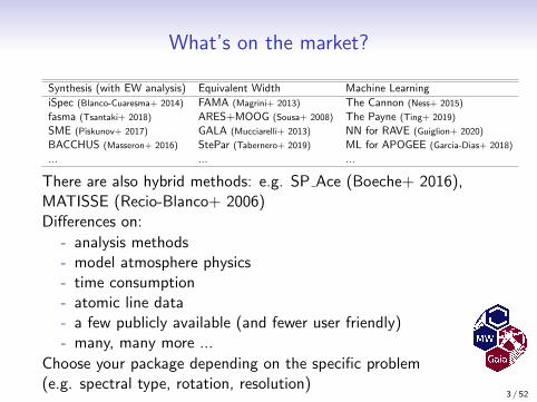
What’s on the market?
Synthesis (with EW analysis) Equivalent Width Machine Learning
iSpec (Blanco-Cuaresma+ 2014) FAMA (Magrini+ 2013) The Cannon (Ness+ 2015)
fasma (Tsantaki+ 2018) ARES+MOOG (Sousa+ 2008) The Payne (Ting+ 2019)
SME (Piskunov+ 2017) GALA (Mucciarelli+ 2013) NN for RAVE (Guiglion+ 2020)
BACCHUS (Masseron+ 2016) StePar (Tabernero+ 2019) ML for APOGEE (Garcia-Dias+ 2018)
... ... ...
There are also hybrid methods: e.g. SP Ace (Boeche+ 2016),MATISSE (Recio-Blanco+ 2006)Differences on:
- analysis methods- model atmosphere physics- time consumption- atomic line data- a few publicly available (and fewer user friendly)- many, many more ...
Choose your package depending on the specific problem(e.g. spectral type, rotation, resolution)
3 / 52
1. How to create a synthetic spectrum
4 / 52
1. How to get the flux at the top of the photosphere
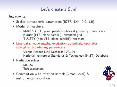
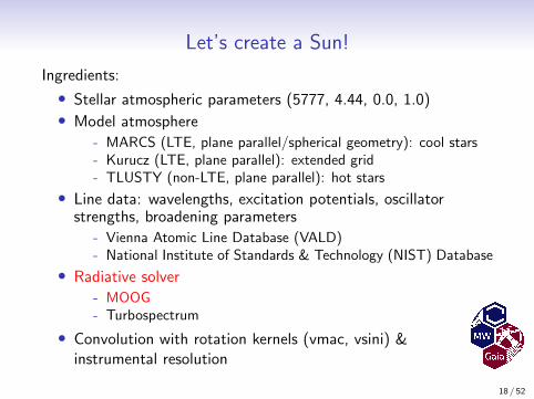
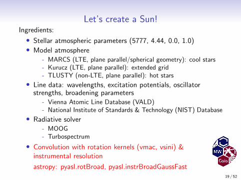
Ingredients:
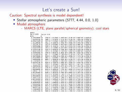
• Stellar atmospheric parameters (Teff , log g , [M/H], vmic)• Model atmosphere
+ optical depth at standard wavelengths+ temperature in K+ number density of free electrons+ number density of all other particles= Calculate the radiative transfer equation → Flux
10 / 52
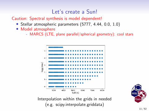
Let’s create a Sun!Caution: Spectral synthesis is model dependent!• Stellar atmospheric parameters (5777, 4.44, 0.0, 1.0)• Model atmosphere
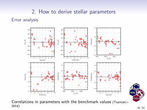
Correlations in parameters with the benchmark values (Tsantaki+2014)
36 / 52
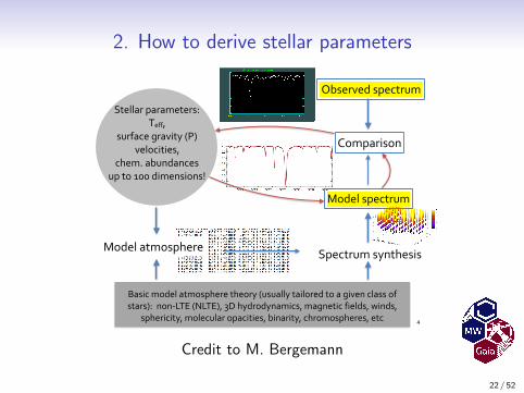
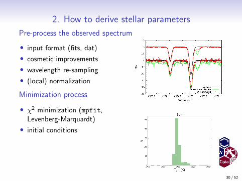
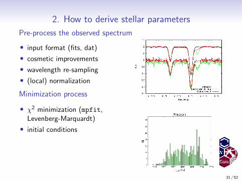
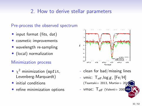
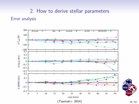
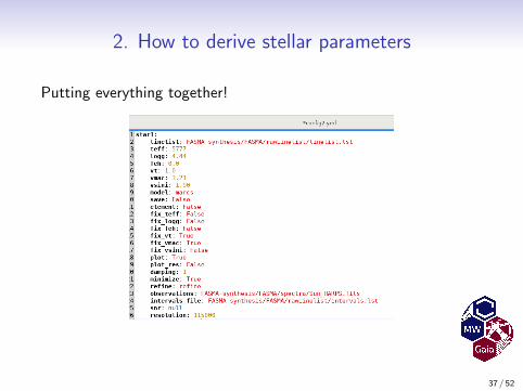
2. How to derive stellar parameters
Putting everything together!
37 / 52
Questions?
38 / 52
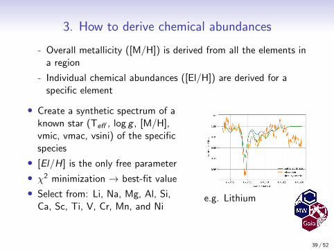
3. How to derive chemical abundances
- Overall metallicity ([M/H]) is derived from all the elements ina region
- Individual chemical abundances ([El/H]) are derived for aspecific element
• Create a synthetic spectrum of aknown star (Teff , log g , [M/H],vmic, vmac, vsini) of the specificspecies
• [El/H] is the only free parameter
• χ2 minimization → best-fit value
• Select from: Li, Na, Mg, Al, Si,Ca, Sc, Ti, V, Cr, Mn, and Ni
e.g. Lithium
39 / 52
3. How to derive chemical abundances
Putting all together!
40 / 52
Questions?
41 / 52
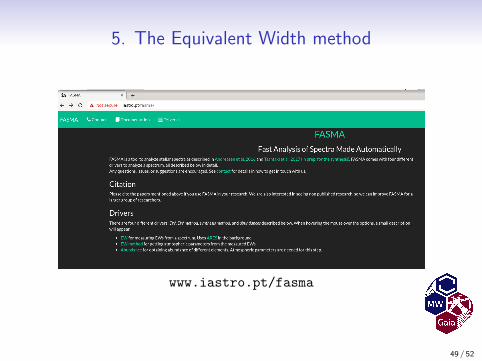
5. The Equivalent Width method
Ingredients:
• Line list of neutral (FeI) and ionized species (FeII)
• EW measurements (IRAF, daospec, ARES)
• Calculate [Fe/H] from the curve of growth
• Model atmospheres (MARCS, Kurucz)
• excitation balance of FeI lines → Teff
ionization balance of FeI and FeII lines → log g
42 / 52
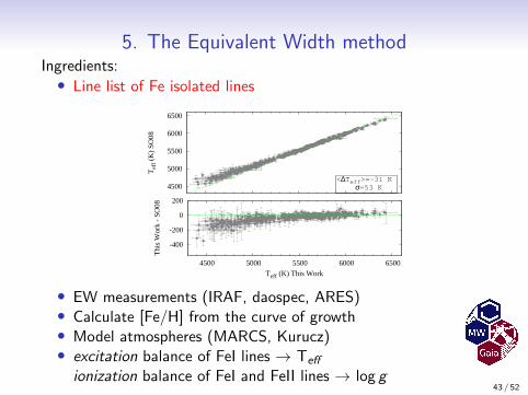
5. The Equivalent Width methodIngredients:• Line list of Fe isolated lines
-400
-200
0
200
4500 5000 5500 6000 6500
Thi
s W
ork
- SO
08
Teff (K) This Work
4500
5000
5500
6000
6500
Tef
f (K
) SO
08
<∆Teff
>=-31 K
σ=53 K
• EW measurements (IRAF, daospec, ARES)• Calculate [Fe/H] from the curve of growth• Model atmospheres (MARCS, Kurucz)• excitation balance of FeI lines → Teff
ionization balance of FeI and FeII lines → log g43 / 52
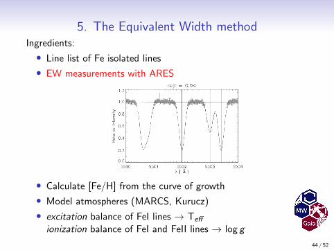
5. The Equivalent Width methodIngredients:
• Line list of Fe isolated lines
• EW measurements with ARES
• Calculate [Fe/H] from the curve of growth
• Model atmospheres (MARCS, Kurucz)
• excitation balance of FeI lines → Teff
ionization balance of FeI and FeII lines → log g
44 / 52
5. The Equivalent Width method
Ingredients:
• Line list of Fe isolated lines
• EW measurements with ARES
• Calculate [Fe/H] from the curve of growth: MOOG+MARCS
• excitation balance of FeI lines → Teff
ionization balance of FeI and FeII lines → log g
45 / 52
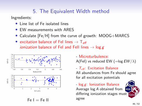
5. The Equivalent Width methodIngredients:
• Line list of Fe isolated lines
• EW measurements with ARES
• Calculate [Fe/H] from the curve of growth: MOOG+MARCS
• excitation balance of FeI lines → Teff
ionization balance of FeI and FeII lines → log g
7.1 7.2 7.3 7.4 7.5 7.6 7.7 7.8
0 1 2 3 4 5
A(F
e I)
E.P. (eV)
7.1 7.2 7.3 7.4 7.5 7.6 7.7 7.8
-5.8 -5.6 -5.4 -5.2 -5 -4.8 -4.6
A(F
e I)
Reduced EW
Fe I = Fe II
- Microturbulence:A(FeI) vs reduced EW (=log EW /λ)
- Teff : Excitation BalanceAll abundances from Fe should agreefor all excitation potentials
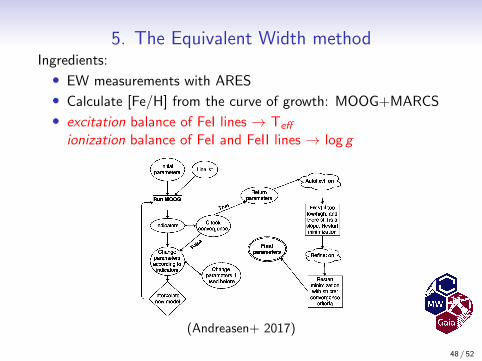
5. The Equivalent Width methodIngredients:• EW measurements with ARES• Calculate [Fe/H] from the curve of growth: MOOG+MARCS• excitation balance of FeI lines → Teff
ionization balance of FeI and FeII lines → log g
(Andreasen+ 2017)47 / 52
5. The Equivalent Width methodIngredients:
• EW measurements with ARES
• Calculate [Fe/H] from the curve of growth: MOOG+MARCS
• Atomic data / Line lists- NIST (Kramida+ 2020)- VALD (Ryabchikova+ 2015)- Kurucz (Kurucz 1995)- Surveys: Gaia-ESO, APOGEE- Specific for K-type (Tsantaki+