Accepted Manuscript

A Health Evaluation Method of Multicopters Modeled by Stochastic Hybrid System

Zhiyao Zhao, Quan Quan, Kai-Yuan Cai

PII: S1270-9638(17)30825-8DOI: http://dx.doi.org/10.1016/j.ast.2017.05.011Reference: AESCTE 4024

To appear in: Aerospace Science and Technology

Received date: 25 January 2016Revised date: 29 January 2017Accepted date: 4 May 2017

Please cite this article in press as: Z. Zhao et al., A Health Evaluation Method of Multicopters Modeled by Stochastic Hybrid System,Aerosp. Sci. Technol. (2017), http://dx.doi.org/10.1016/j.ast.2017.05.011

This is a PDF file of an unedited manuscript that has been accepted for publication. As a service to our customers we are providingthis early version of the manuscript. The manuscript will undergo copyediting, typesetting, and review of the resulting proof before it ispublished in its final form. Please note that during the production process errors may be discovered which could affect the content, and alllegal disclaimers that apply to the journal pertain.

1

A Health Evaluation Method of Multicopters

Modeled by Stochastic Hybrid SystemZhiyao Zhao*, Quan Quan, and Kai-Yuan Cai

Abstract

For multicopters, failures may abort missions, crash multicopters, and moreover, injure or even kill people.

In order to guarantee flight safety, a system of prognostics and health management should be designed to

prevent or mitigate unsafe consequences of multicopter failures, where health evaluation is an indispensable

module. This paper proposes a health evaluation method of multicopters based on Stochastic Hybrid System

(SHS). In the SHS model, different working conditions (health statuses) of multicopters are modeled as discrete

states, and system behaviors of different working conditions are modeled as continuous dynamics under discrete

states. Then, the health of multicopters is quantitatively measured by a definition of health degree, which is

a probability measure describing an extent of system degradation from an expected normal condition. On this

basis, the problem of multicopter’s health evaluation is transformed to a hybrid state estimation problem. In this

case, a modified interacting-multiple-model algorithm is proposed to estimate the real-time distribution of hybrid

state, and evaluate multicopter’s health. Finally, a case study of multicopter with sensor anomalies is presented

to validate the effectiveness of the proposed method.

Index Terms

Health evaluation, multicopter, stochastic hybrid system, interacting multiple model, health degree, sensor

anomaly.

This work is supported by the National Natural Science Foundation of China (Grant No. 61473012 and No. 61603014)

The authors are with School of Automation Science and Electrical Engineering, Beihang University, Beijing 100191, China (e-mail:

zzy buaa@buaa.edu.cn; qq buaa@buaa.edu.cn; kycai@buaa.edu.cn)

May 10, 2017 DRAFT

2

NOTATION

x Process variable vector

y Observation

px, py, pz Multicopter’s position in the earth-fixed frame

w,Γw,Q Process noise, its covariance matrix and driven matrix

v,Γv,R Measurement noise, its covariance matrix and driven matrix

q Discrete state

f (·) Probability density distribution

H (·) Health degree

P {·} Probability measure

Tr Mission trajectory

Π Transition probability matrix

π Transition probability

x Estimate of x

P Covariance matrix of x

T Sample time

N (·) Gaussian distribution

I. INTRODUCTION

A. Motivation and outline

Multicopters have attracted close attention in the field of aircraft engineering. They are well-suited to a wide

range of mission scenarios, such as search and rescue [1], [2], package delivery [3], border patrol [4], military

surveillance [3], [5] and agricultural application [6], [7]. From a safety perspective, multicopter failures cannot

be absolutely avoided, including communication breakdown, sensor failure and propulsion system anomaly, etc.

These failures may abort missions, crash multicopters, and moreover, injure or even kill people. In order to

guarantee flight safety, a system of Prognostics and Health Management (PHM) should be designed to prevent

or mitigate unsafe consequences caused by multicopter failures [8]. As shown in Fig. 1, health evaluation is

a key component in the PHM system, which has been highly concerned in the field of system engineering

[9]-[12]. Information obtained from health evaluation can be used to understand the system behavior, also as a

reference for operating a safety decision-making [13].

The current research of health evaluation commonly focuses on a component level [14]. Fault diagnosis

[15]-[19] and fault-tolerant control [20]-[25] related to specific components have been extensively studied

for enhancing the flight safety of aircrafts. Different from fault diagnosis, health evaluation research should

concentrate on a performance of the whole aircraft rather than a fault occurred in local onboard components

[12], [26]. For multicopters, different onboard components such as actuators and sensors are correlated through

the autopilot. Sensor measurements are sent to the autopilot, analyzed in the autopilot, and then the control

instructions are sent to actuators from the autopilot. In this case, the health of multicopters cannot only consider

onboard component faults, but also the whole system behavior directed by the autopilot. However, there is little

May 10, 2017 DRAFT

3

Plant

Sensing apparatus

Observed behavior

Management

Prediction

Evaluation

PHMsystem

Fig. 1. PHM framework.

study concerning multicopter’s health evaluation from a system behavior perspective. The main reason lies in

two aspects: 1) a quantitative definition of system health is lacked. Residuals are always viewed as a quantitative

index to characterize a fault [27]-[30] in fault diagnosis research, while PHM research always uses different

kinds of physical and mathematical quantities as health indicators, such as sensor measurements [31], [32],

features [33], [34] and reliability indices [35]-[38]. However, a unified mathematical definition to describe and

quantitatively measure system health is lacked and required to be proposed. 2) A multicopter model for both

health evaluation and safety decision-making research is lacked. The current research always separately studied

health evaluation and safety decision-making of multicopters by using different models. Actually, accurate health

evaluation is a key premise of correct safety decision-making, while safety decision-making is the final purpose

of health evaluation. Thus, it is required to study a model which can be used for both health evaluation and

safety decision-making research.

Stochastic Hybrid System (SHS) can be used to analyze and design complex systems that operate in the

presence of uncertainties, and contain multiple working modes [39]-[41]. It can model multicopter’s dynamic

behavior and performance degradation, because it interacts continuous dynamics and discrete dynamics [42],

[43]. These characteristics enable SHS to be used in designing multicopter’s autopilot for the purpose of both

health evaluation and safety decision-making. In this case, this paper proposes an SHS-based health evaluation

method for multicopters. In the SHS model, different working conditions (health statuses) of multicopters are

modeled as discrete states, and system behaviors of different working conditions are modeled as continuous

dynamics under discrete states. Then, the health of multicopters is quantitatively measured by a definition of

health degree, which is a probability measure describing an extent of system degradation from an expected

normal condition. On this basis, the problem of multicopter’s health evaluation is transformed to a hybrid state

estimation problem. In this case, a modified interacting-multiple-model (IMM) algorithm is proposed to estimate

the real-time distribution of hybrid state, and the health degree is further calculated. Finally, a case study of a

multicopter with sensor anomalies is simulated to validate the effectiveness of the proposed method, and some

comparative studies are also made and discussed.

May 10, 2017 DRAFT

4

B. Related work

The UAV health can be characterized into four categories [14]:

1) Structure/Actuator health. This category focuses on damage of structure and actuator components of UAVs.

For structure health, flight data and vibration signals from airframe including wings [44], [45], blades [46] and

tail booms [47] are usually collected and analyzed by data-driven approaches to detect anomalies in both time

and frequency domain [48]. For actuator health, filtering-based methods are always used to estimate an additive

fault [49], [50] or a degradation of control efficiency [51], where residuals [27]-[30] and controllability index

[52] are viewed as health indices. On this basis, fault-tolerant algorithms dealt with such failures [20]-[25] are

widely studied.

2) Sensor health. This category focuses on failure of onboard sensor-hardwares such as barometers, gyro-

scopes, etc. Sensor failure may include loss of signal, signal stuck, drift, big noise interference, etc. Similar as

actuators, the health evaluation of sensors can be also based on observers and filtering-based methods [53]-[55].

Meanwhile, data-driven approaches [56] and fusion approaches [57], [58] are also proposed to detect sensor

faults. Based on fault detection results, fault-tolerant algorithms dealt with such a failure [59], [60] are also

studied.

3) Communication health. This category concentrates on the functionality of the signal transmission between

the UAV and the remote controller or ground control station, even among multiple UAVs. Interference, loss

of contact and degraded contact quality are commonly appeared during flight. In this area, most works study

the decision-making, coordination and cooperation of a UAV team when communication anomaly occurs [61].

Meanwhile, there exists research about mission planning for communication constraint situation [5]. In addition,

civilian-purposed UAVs are vulnerable to malicious data interference. This leads to a game-theoretical analysis

of attack and anti-attack of UAVs by using communication channels [62]-[64].

4) Fuel health. Battery is commonly-seen as a power source of small UAVs. State-of charge and state-of-

health are two indices reflecting the remaining capacity and residual life of batteries [65]. There exists amounts

of research on the evaluation and prediction of these indices [66]-[69]. For safety and reliability purpose, battery

management system is also studied and developed [70]-[72]. For other type of fuel, the emphasis is on the

mission planning when the fuel quantity drops below a certain threshold [73], [74].

To sum up, the existed PHM methods of UAVs are mainly focused on the fault detection and identification at

the component level and the corresponding mission planning scheme. In these methods, sensor measurements,

features, residuals and reliability indices are used as health indicators. Different from the mentioned research,

this paper introduces a concept of health degree as a unified health indicator to evaluate health of multicopters,

where the value quantitatively reflects the performance deviation from the expected normal condition. Since

the health degree is calculated based on the distribution of system process (continuous) variables, the proposed

method is a health evaluation method at a system behavior level.

The remainder of this paper is organized as follows. Section II proposes an SHS-based model of multicopters,

and quantitatively defines its health by introducing the definition of health degree. Section III proposes a modified

IMM algorithm to evaluate the health of the multicopter. Section IV presents a case study of multicopter with

sensor anomalies to validate the effectiveness and advantages of the proposed health evaluation method, where

simulation results are given and discussed. Section V gives a conclusion, and indicates future development of

May 10, 2017 DRAFT

5

the proposed method.

II. AN SHS-BASED MODELING OF MULTICOPTER AND ITS HEALTH DEFINITION

In this section, preliminaries of discrete-time SHS model [40]-[43] are presented. Then, two kinds of models,

namely “Stochastic Continuous System (SCS)-based model” and “SHS-based model”, are presented to model

the multicopter for the purpose of health evaluation. On this basis, a health definition of multicopters is proposed.

A. Preliminaries

Let (Ω,F ,Ft,P) be a complete probability space with a sample space Ω, a σ-field of the events F , a natural

filtration Ft and a natural probability measure P : F −→ [0, 1]. Let B (·) denotes the Borel σ-algebra.

Definition 1. In the probability space (Ω,F ,Ft,P), a general discrete-time SHS model is a tuple H =

(Q, n, Init, Tx, Tq, R), which is detailed as follows:

1) Q : = {q1, q2, · · · , qm} is a finite set of discrete states for m ∈ N.

2) n : Q −→ N which assigns each discrete state q ∈ Q a continuous state space Rn(q). Then, the hybrid

state s = (q,x) is defined in the hybrid state space S = Q×Rn(q).

3) Init : B (S)−→ [0, 1] represents the initial distribution of the hybrid state space S.

4) Tx : B (R

n(·))× S −→ [0, 1] is a Borel-measurable stochastic kernel on Rn(·) given S, which assigns to

each s ∈ S a probability measure on the Borel space(R

n(q),B (R

n(q)))

: Tx (· |s ).5) Tq : Q × S −→ [0, 1] is a discrete stochastic kernel on Q given S, which assigns to each s ∈ S a

probability distribution over Q : Tq (· |s ).6) R : B (

Rn(·))×S ×Q −→ [0, 1] is a Borel-measurable stochastic kernel on R

n(·) given S ×Q, that assigns

to each s ∈ S, and q′ ∈ Q a probability measure on the Borel space(R

n(q′),B(R

n(q′)))

: R (· |s, q′ ).

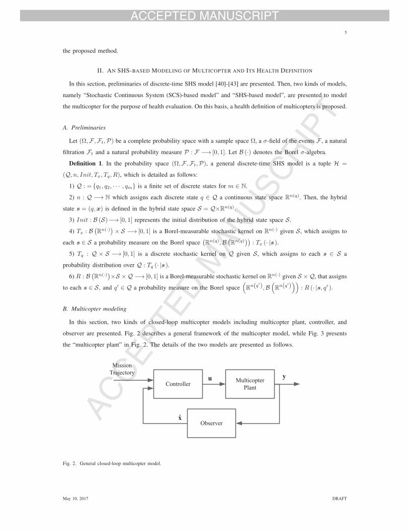
B. Multicopter modeling

In this section, two kinds of closed-loop multicopter models including multicopter plant, controller, and

observer are presented. Fig. 2 describes a general framework of the multicopter model, while Fig. 3 presents

the “multicopter plant” in Fig. 2. The details of the two models are presented as follows.

Controller MulticopterPlant

Observer

MissionTrajectory

u

x

y

Fig. 2. General closed-loop multicopter model.

May 10, 2017 DRAFT

6

� � � � � �� � � �� � � � � �

2 2,

2

2

22 ,

1 ,

1

k k k k

k k k

� � �

� � �w

v

x f x u w

y x v

Γ

C Γ

2 : GPS anomaly stateq

� � � � � �� � � �� � � � � �

1 1,

1

1

11 ,

1 ,

1

k k k k

k k k

� � �

� � �w

v

x f x u w

y x v

Γ

C Γ

1 : fully healthy stateq

� � � � � �� � � �� � � � � �

3 3,

3

3

33 ,

1 ,

1

k k k k

k k k

� � �

� � �w

v

x f x u w

y x v

Γ

C Γ

3 : barometer anomaly stateq� � � � � �� � � �� � � � � �

4 4,

4

4

44 ,

1 ,

1

k k k k

k k k

� � �

� � �w

v

x f x u w

y x v

Γ

C Γ

4 : compass anomaly stateq

11�21� 12�

22�

24�

44�

42�

33�

23�

32�

31�13�

34�

43�

14� 41�

� � � � � �� � � �� � � � � �

1 ,

1

k k k k

k k k

� � �

� � �w

v

x f x u w

y x v

Γ

C Γ

(a) SCS-based model plant (b) SHS-based model plant

Fig. 3. Model plant.

1) SCS-based model: Scholars have studied the dynamics of multicopters [49], [50], [75]-[77]. Equation (1)

presents a general dynamic model:

px = vx

py = vy

pz = vz

vx = −uz (cosφ sin θ cosψ + sinφ sinψ) /m

vy = −uz (cosφ sin θ sinψ − sinφ cosψ) /m

vz = −uz cosφ cos θ/m+ g

φ = vφ + tan θ (vψ cosφ+ vθ sinφ)

θ = vθ cosφ− vψ sinφ

ψ = sec θ (vψ cosφ+ vθ sinφ)

vφ = (Jy − Jz) vψvθ/Jx + uφ/Jx

vθ = (Jz − Jx) vφvψ/Jy + uθ/Jy

vψ = (Jx − Jy) vφvθ/Jz + uψ/Jz︸ ︷︷ ︸x = G (x,u)

(1)

where the vector x = (px, py, pz, vx, vy, vz, φ, θ, ψ, vφ, vθ, vψ)T ∈ R

12×1 contains process variables of the

multicopter. The components px, py, pz represent the multicopter’s position in the earth-fixed frame; the com-

ponents vx, vy, vz represent the multicopter’s velocity in the earth-fixed frame; the components φ, θ, ψ represent

May 10, 2017 DRAFT

7

the angles of roll, pitch and yaw, respectively; the components vφ, vθ, vψ represent the angular velocity of φ, θ, ψ,

respectively; The parameters Jx, Jy, Jz are the moments of inertia along x, y, z directions, respectively; m is

the mass of the multicopter; g is the acceleration of gravity. The positive direction of z-axis of the earth-fixed

frame points to the ground. The control input u = [uz, uφ, uθ, uψ]T includes a total lift and moments of angles

φ, θ, ψ, respectively.

With the estimated x by a designed observer and an expected control target xd = [px,d, py,d, pz,d, ψd]T, the

control input u = [uz, uφ, uθ, uψ]T can be calculated by a PD controller as

uz = −kP,z (pz,d − pz) + kD,z vz +mg

uφ = kP,φ

(φd − φ

)− kD,φvφ

uθ = kP,θ

(θd − θ

)− kD,θvθ

uψ = kP,ψ

(ψd − ψ

)− kD,ψ vψ,

(2)

where ⎡⎣ θd

φd

⎤⎦ = g−1

⎛⎝ cos ψ sin ψ

sin ψ − cos ψ

⎞⎠

−1⎛⎝KPa

⎡⎣ px − px,d

py − py,d

⎤⎦+KDa

⎡⎣ vx

vy

⎤⎦⎞⎠ . (3)

Equations (2) and (3) describe a position controller of the multicopter. To obtain the discrete-time dynamic

model of the multicopter, equation (1) is discretized through the Euler method [78] as

x (k) = x (k − 1) + TG (x (k − 1) ,u (k)) , (4)

where T is the discretized time. Combining (4) with an observation equation and related noise items, we have

x (k) = f (x (k − 1) ,u (k)) + Γww (k)

y (k) = Cx (k − 1) + Γvv (k)(5)

where the function f (x (k − 1) ,u (k)) = x (k − 1) + TG (x (k − 1) ,u (k)) ; the vector y contains system

measurements, and C is the corresponding parameter matrix. Without loss of generality, let C = I12 be an

identity matrix, which means all process variables are directly measured. The items w and v are the process

noise and measurement noise, satisfying that⎧⎨⎩

w (·) ∼ N (0,Q) ,v (·) ∼ N (0,R) , ∀kcov [w (k) ,v (j)] = E

[w (k)vT (j)

]= 0, ∀k, j

, (6)

where Q and R are the covariance matrices. The matrices Γw and Γv are the corresponding noise driven

matrices. Note that equation (5) is a discrete-time stochastic continuous (variable) system.

Remark 1. The presented model in this part, namely “SCS-based model”, only models the multicopter system

when the multicopter is in a fully healthy status. However, for the purpose of health evaluation, the multicopter

contains different health statuses, where transitions might occur among them. Considering the SHS model has

discrete dynamics as well as continuous dynamics, an SHS-based multicopter is presented for the purpose of

health evaluation.

2) SHS-based model: An SHS-based multicopter model is constructed as shown in Fig. 3(b). For simplicity,

we have two assumptions as follows.

Assumption 1. Sensors including GPS, barometer and compass are considered to be possibly unhealthy in

the SHS-based model. The other onboard components such as propulsion system, communication system and

other sensors are all considered to be healthy.

May 10, 2017 DRAFT

8

Assumption 2. There will be at most one anomaly occurred in either GPS, barometer or compass at the

same time, which means it is impossible that two sensors are simultaneously unhealthy.

Remark 2. Assumption 1 confines the discrete dimension of the SHS-based model, which leads to convenient

understanding of the SHS-based model structure and the subsequent health evaluation algorithm. Assumption

2 also confines the discrete dimension. This is reasonable, because there is little chance that two sensors are

both unhealthy at the same time for a qualified multicopter product. Actually, Assumptions 1&2 can be relaxed

by introducing more discrete states of SHS (health statuses). This relaxation has little influence on the health

evaluation algorithm.

According to Assumptions 1&2, four discrete states are considered in the SHS-based multicopter model.

Following Definition 1, we have

Q = {q1, q2, q3, q4} ,

where q1 is a fully healthy status, q2 is a GPS anomaly status, q3 is a barometer anomaly status, and q4 is a

compass anomaly status, respectively. For ∀qj ∈ Q, the continuous dynamics is

x (k) = f j (x (k − 1) ,u (k)) + Γw,jwj (k)

y (k) = Cjx (k − 1) + Γv,jvj (k), (7)

where ⎧⎪⎪⎪⎨⎪⎪⎪⎩

f1 (·) = f2 (·) = f3 (·) = f4 (·) = f

Γw,1 = Γw,2 = Γw,3 = Γw,4 = Γw

f (w1) = f (w2) = f (w3) = f (w4) = f (w)

.

The symbol f (w) is the probability density function (pdf) of w. Note that f j (·) contains the controller same

as (2). As to the observation equation, for state q1, we have⎧⎪⎪⎪⎪⎪⎪⎪⎪⎪⎨⎪⎪⎪⎪⎪⎪⎪⎪⎪⎩

C1 =

⎡⎢⎢⎢⎢⎢⎢⎣

c1

c2...

c12

⎤⎥⎥⎥⎥⎥⎥⎦

Γv,1 = Γv

, (8)

where ci is the ith row vector of C1. For state q2 representing GPS anomaly, the components {px, py} of x

may be incorrectly measured, even the GPS measurements are completely lost. Then, we have

C2 = C1\⎡⎣ c1

c2

⎤⎦ , (9)

which is interpreted that C2 is the rest part of subtracting the rows c1 and c2 from C1. The meaning of C2 is

that when a GPS anomaly occurs, the continuous dynamics under state q2 does not consider GPS measurements,

despite whether the GPS can generate measurements or not. According to this principle, for states q3 and q4,

we haveC3 = C1\e3C4 = C1\e9

, (10)

because the height pz and the yaw angle ψ are the 3rd and 9th components of x, respectively. The observation

noise v and the corresponding noise driven matrix Γv under states q2, q3 and q4 can be also obtained following

the similar variation of the matrix Cj .

May 10, 2017 DRAFT

9

It should be indicated that (7) determines the stochastic kernel Tx (· |s ). Note that the stochastic kernel

Tx (· |s ) is different for different health statuses, because the forms of Cj and Γv,jvj are inconsistent for

different health statuses. For the stochastic kernel Tq (· |s ), it reflects the transitions among different health

statuses. Here, the discrete dynamics is a first-order Markov chain with transition probabilities as

P {qj (k + 1) |qi (k)} = πij (k) , ∀qi, qj ∈ Q,

andm∑j=1

πij (k) = 1, i = 1, 2, · · · ,m.

The failure rate or anomaly rate of onboard components in a multicopter and the related reliability test data

are helpful for determining the value of the transition probability πij . For the stochastic kernel R (· |s, q′ ), we

can let R (· |s, q′ ) = Tx (· |s ). This indicates that during the time step when the discrete transition occurs, the

system process variables keep evolving according to the continuous dynamics of the previous discrete state

before the transition.

Up to now, two kinds of multicopter model are presented. Table I summarizes the model information presented

in this section.

Table I Multicopter model information

Type SCS-based model SHS-based model

Plant described in (5) and Fig. 3(a) described in (7) and Fig. 3(b)

Controller described in (2)&(3) described in (2)&(3)

Observer Extended Kalman Filter (EKF) a modified IMM-based algorithm

Remark 3. The sub-model of state q1 in the SHS-based model is an SCS-based model. This indicates that

the SHS-based model is a more general model, which fits the requirement of health evaluation.

Remark 4. The SHS-based model can be extended for considering more kinds of unhealthy situations. For

example, other sensors such as gyroscope anomaly can be also modeled as a new health status following the

principles above. For propulsion system anomaly, especially for actuator anomaly, the form of the nonlinear

function f (·) with a control effectiveness matrix and the noise item Γww can be modified to generate new

health statuses.

C. Health definition

In order to quantitatively evaluate the performance of the multicopter, a definition of the health degree

is proposed for a multicopter. “Health” can be defined as an extent of system degradation or performance

deviation from an expected normal condition [79]. A dynamical system is considered healthy if suitable for its

intended purpose for an extended period of time and considered unhealthy if damaged or approaching a status

of failure for its intended purpose [80]. In this case, an mathematical definition of health degree is proposed

for a multicopter by referring to the safety assessment in SHS theory [40], [41] and the real-time reliability

evaluation in reliability theory [35]-[37].

A multicopter is always expected to execute a mission from the assignment of users. The mission can be

described by a sequence of waypoints, indicating a mission trajectory. From a perspective of health of dynamical

May 10, 2017 DRAFT

10

systems, a multicopter is considered healthy if it flies following the trajectory without deviation. Thus, the health

degree is defined as a probability that the multicopter follows the mission trajectory. Suppose a multicopter has a

predefined mission trajectory Tr ={(

pMx , pMy , pMz), k

∣∣(pMx (k) , pMy (k) , pMz (k)) ∈ R

3, for k = 0, 1, 2, · · · } .Then, we propose definitions of instantaneous health degree and interval health degree.

Predefined missiontrajectory rT

radius:�

Fig. 4. Diagram of the predefined mission trajectory Tr and the tolerant threshold ε.

Definition 2 (Instantaneous health degree). Given a mission trajectory Tr and the real position (px (k) , py (k) , pz (k))

of a multicopter at time k. Let

Δp (k) =∥∥(px (k) , py (k) , pz (k))− (

pMx (k) , pMy (k) , pMz (k))∥∥

2.

The instantaneous health degree at time k is defined as

H (k) = P {Δp (k) � ε |∀qj ∈ Q} , (11)

where ε > 0 represents the tolerant threshold of behavior deviation caused by anomalies as shown in Fig. 4.

Definition 3 (Interval health degree). Given a mission trajectory Tr and the real position (px, py, pz) of a

multicopter over a time interval [k1, k2]. The interval health degree over a time interval [k1, k2] is defined as

H (k1, k2) = P {Δp (j) � ε, ∀j ∈ [k1, k2] |∀qj ∈ Q} . (12)

Remark 5. As shown in Fig. 4, the envelope generated by the mission trajectory Tr and the tolerant threshold

ε is called as a health set, which is similar as the safe set definition in the safety assessment research. For an

assigned mission, its trajectory is predefined and known, and the tolerant threshold ε should be appropriately

selected based on specific user requirements and engineering experience. On this basis, the instantaneous health

degree is the probability that the multicopter remains within the health set at time k, no matter which discrete

state it belongs to. It uses an instantaneous behavior of multicopter to measure its health, and the health

degradation can be obtained immediately after the anomaly occurs. Furthermore, the interval health degree is

the probability that the multicopter remains within the health set over the time interval [k1, k2], no matter which

discrete state it belongs to. It focuses on a behavior over a time interval to evaluate system health, and it treats

system health as a process indicator representing system features over a time interval. Both the definitions have

their own advantages.

May 10, 2017 DRAFT

11

III. HEALTH EVALUATION OF MULTICOPTER

A. Problem formulation

For the presented SHS-based multicopter model H = (Q, n, Init, Tx, Tq, R) , an initial distribution of the

hybrid state s (0) = (q (0) ,x (0)) can be described as⎧⎨⎩

f (x (0) |qj (0) ) = N (xj (0) ,Pj (0))

P {qj (0)} = μj (0), j = 1, 2, · · · ,m,

where μj (0) � 0 for ∀qj ∈ Q, and∑m

j=1 μj (0) = 1. Let Yk = {y (0) ,y (1) , · · · ,y (k)} represent the

sequence of sensor measurements up to time k. In order to calculate the health degree at time k by Definition

2, the distribution of the hybrid state s should be accurately estimated, including the pdf f(x (k)

∣∣qj (k) ,Yk)

(i.e. distribution of process variables x (k) conditional on discrete state qj (k) and Yk) and the discrete state

probability P (q (k)

∣∣Yk). By the theorem of total probability, we have

f(x (k)

∣∣Yk)=

m∑j=1

f(x (k)

∣∣qj (k) ,Yk) · Pj

(qj (k)

∣∣Yk). (13)

Then, the health degree at time k is calculated as

H (k) =

∫Ω

f(x (k)

∣∣Yk)dx, (14)

where Ω is a polyhedron with a center(pMx (k) , pMy (k) , pMz (k)

)and a radius ε. For the health degree over a

time interval [k1, k2], assuming the time index conforms to uniform distribution for simplicity, we have

H (k1, k2) =k2∑

i=k1

H (i)

k2 − k1. (15)

According to (13)-(15), the key of the health degree calculation is to accurately estimate the distribution

of the hybrid state s. In this case, an IMM-based algorithm [81] is employed here to achieve hybrid state

estimation.

B. IMM-based health evaluation

1) Classic IMM algorithm: The classic IMM algorithm is a recursive estimator [81]. In each recursive cycle,

it consists of four major steps: 1) model-conditional reinitialization (interacting or mixing of the estimates),

where the input to the filter of each mode is obtained by mixing the estimates of all filters at the previous

time under the assumption that the system is in this particular mode at the present time; 2) model-conditional

filtering, performed in parallel for each mode; 3) mode probability update, based on the model-conditional

likelihood functions; 4) estimate fusion, which yields the overall state estimate as the weighted sum of the

updated state estimates of all filters. The procedure of the classic IMM algorithm is shown in Table II. Note

that the concept of mode in the IMM algorithm corresponds to the concept of discrete states in the SHS-based

multicopter model.

Remark 6. For performing the classic IMM algorithm on the health evaluation of a multicopter with the

SHS-based model, there are two deficiencies which are required to be modified. i) In the classic IMM algorithm,

the transition probability is assumed to be constant over the studied time interval, and the transition probability

from any particular anomaly mode to the normal mode is generally and artificially set larger than others in order

to prevent a false fault diagnosis [82]. However, the unchanged transition probability can mislead the mode

May 10, 2017 DRAFT

12

identification to intermittently declare a false alarm, especially when a fault-tolerant controller works well after

the first anomaly occurs. This is because the model probability of the healthy mode tends to increase again

as the current anomalous system converges to a steady state by the fault-tolerant control law after an anomaly

occurs [83]. ii) Following the classic IMM algorithm, the real-time distribution of f(x (k)

∣∣qj (k) ,Yk)

cannot

be approximated as a Gaussian distribution, because the mixing covariance in Step 1 will change the covariance

of x under mode qj in a non-Gaussian way. This will lead to a difficulty in the health degree calculation due

to a non-Gaussian distribution of f(x (k)

∣∣qj (k) ,Yk).

In this case, two modifications are made to the classic IMM algorithm, and the health evaluation algorithm

based on the modified IMM algorithm is proposed as follows.

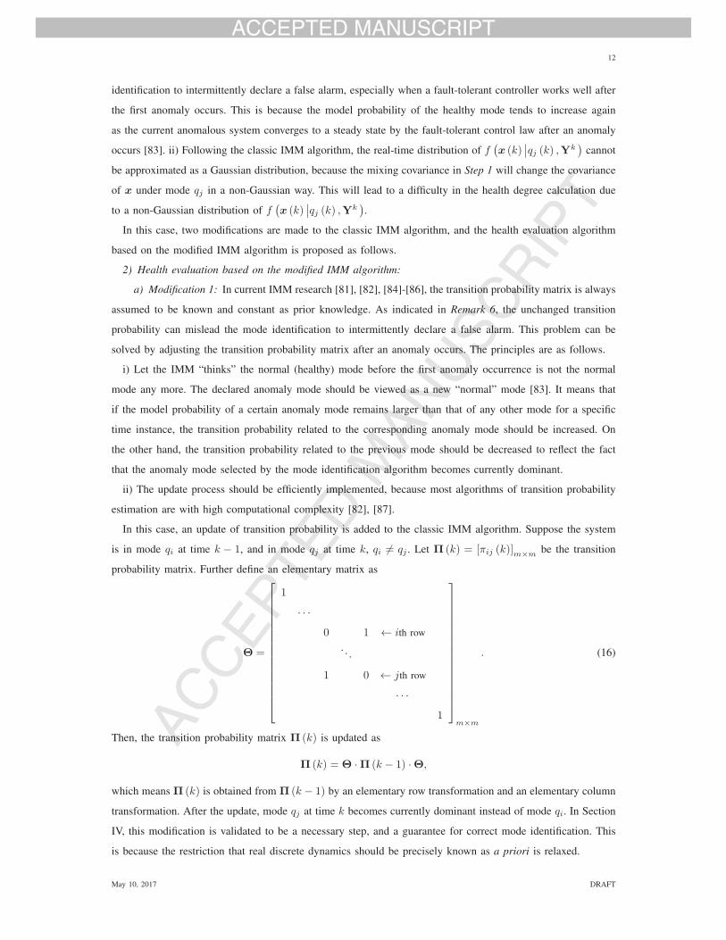
2) Health evaluation based on the modified IMM algorithm:

a) Modification 1: In current IMM research [81], [82], [84]-[86], the transition probability matrix is always

assumed to be known and constant as prior knowledge. As indicated in Remark 6, the unchanged transition

probability can mislead the mode identification to intermittently declare a false alarm. This problem can be

solved by adjusting the transition probability matrix after an anomaly occurs. The principles are as follows.

i) Let the IMM “thinks” the normal (healthy) mode before the first anomaly occurrence is not the normal

mode any more. The declared anomaly mode should be viewed as a new “normal” mode [83]. It means that

if the model probability of a certain anomaly mode remains larger than that of any other mode for a specific

time instance, the transition probability related to the corresponding anomaly mode should be increased. On

the other hand, the transition probability related to the previous mode should be decreased to reflect the fact

that the anomaly mode selected by the mode identification algorithm becomes currently dominant.

ii) The update process should be efficiently implemented, because most algorithms of transition probability

estimation are with high computational complexity [82], [87].

In this case, an update of transition probability is added to the classic IMM algorithm. Suppose the system

is in mode qi at time k − 1, and in mode qj at time k, qi �= qj . Let Π (k) = [πij (k)]m×m be the transition

probability matrix. Further define an elementary matrix as

Θ =

⎡⎢⎢⎢⎢⎢⎢⎢⎢⎢⎢⎢⎢⎢⎢⎢⎣

1

· · ·0 1 ← ith row

. . .

1 0 ← jth row

· · ·1

⎤⎥⎥⎥⎥⎥⎥⎥⎥⎥⎥⎥⎥⎥⎥⎥⎦m×m

. (16)

Then, the transition probability matrix Π (k) is updated as

Π (k) = Θ ·Π (k − 1) ·Θ,

which means Π (k) is obtained from Π (k − 1) by an elementary row transformation and an elementary column

transformation. After the update, mode qj at time k becomes currently dominant instead of mode qi. In Section

IV, this modification is validated to be a necessary step, and a guarantee for correct mode identification. This

is because the restriction that real discrete dynamics should be precisely known as a priori is relaxed.

May 10, 2017 DRAFT

13

Table II Procedure of the classic IMM algorithm

1. Interacting (for j = 1, 2, · · · ,m)

1) predicted mode probability: μj (k|k − 1) � P {qj (k) |Yk−1

}=∑

i πijμi (k − 1)

2) mixing probability: μi|j (k − 1) � P {qi (k − 1) |qj (k) ,Yk−1

}= πijμi (k − 1) /μj (k|k − 1)

3) mixing estimate: x0j (k − 1|k − 1) � E

[x (k − 1) |qj (k) ,Yk−1

]=∑

i xi (k − 1|k − 1)μi|j (k − 1)

4) mixing covariance: P0j (k − 1|k − 1) �cov

[x0j (k − 1|k − 1)

∣∣qj (k) ,Yk−1]=∑

i [Pi (k − 1|k − 1)

+[x0j (k − 1|k − 1)− xi (k − 1|k − 1)

] [x0j (k − 1|k − 1)− xi (k − 1|k − 1)

]T ]μi|j (k − 1)

2. Model-conditional filtering (for j = 1, 2, · · · ,m)

1) predicted state: xj (k|k − 1) � E[x (k) |qj (k) ,Yk−1

]= f j

(x0j (k − 1|k − 1) ,u (k)

)2) predicted covariance: Pj (k|k − 1) �cov

[xj (k|k − 1)

∣∣qj (k) ,Yk−1]

= Aj (k − 1)P0j (k − 1|k − 1)AT

j (k − 1) + Γw,jQjΓTw,j , where Aj (k − 1) =

∂fj

∂x

∣∣∣x0j (k−1|k−1),u(k)

3) measurement residual: rj � y (k)− E[y (k) |qj (k) ,Yk−1

]= y (k)−Cj (k) xj (k|k − 1)

4) residual covariance: Sj �cov[rj

∣∣qj (k) ,Yk−1]= Cj (k)Pj (k|k − 1)CT

j (k) + Γv,jRjΓTv,j

5) filter gain: Kj = Pj (k|k − 1)CTj (k)S−1

j

6) updated state: xj (k|k) � E[x (k) |qj (k) ,Yk

]= xj (k|k − 1) +Kjrj

7) updated covariance: Pj (k|k) �cov[xj (k|k)

∣∣qj (k) ,Yk]= Pj (k|k − 1)−KjS

Tj Kj

3. Mode probability update (for j = 1, 2, · · · ,m)

1) likelihood function: Lj (k) = N (rj ;0,Sj) =1√

|(2π)Sj |exp

(− 12r

Tj S

−1j rj

)2) mode probability: μj (k) � P {

qj (k) |Yk}=

μj(k|k−1)Lj(k)∑i μi(k|k−1)Li(k)

3) mode estimation: μj (k) = maxi μi (k)

⎧⎨⎩

� μT =⇒ The system is in mode qj

< μT =⇒ No mode is recognized

4. Estimate fusion (for the output purpose)

1) overall estimate: x (k|k) � E[x (k) |Yk

]=∑

j xj (k|k)μj (k)

2) overall covariance: P (k|k) � E[[x (k)− x (k|k)] [x (k)− x (k|k)]T |Yk

]=∑

j

[Pj (k|k) + [x (k|k)− xj (k|k)] [x (k|k)− xj (k|k)]T

]μj (k)

5. k = k + 1

b) Modification 2: As indicated in Remark 6, the real-time distribution of f(x (k)

∣∣qj (k) ,Yk)

cannot

be approximated as a Gaussian distribution following the classic IMM algorithm. In this case, a modification is

performed on the IMM algorithm by let P0j (k − 1|k − 1) = Pj (k − 1|k − 1) in Table II. Actually, without the

covariance mixing process, it will not degrade the performance of the IMM algorithm in our research, which

will be shown in Section IV. Thus, the pdf f(x (k)

∣∣qj (k) ,Yk)

can be approximated as [88], [89]

f(x (k)

∣∣qj (k) ,Yk)= N (xj (k|k) ,Pj (k|k)) .

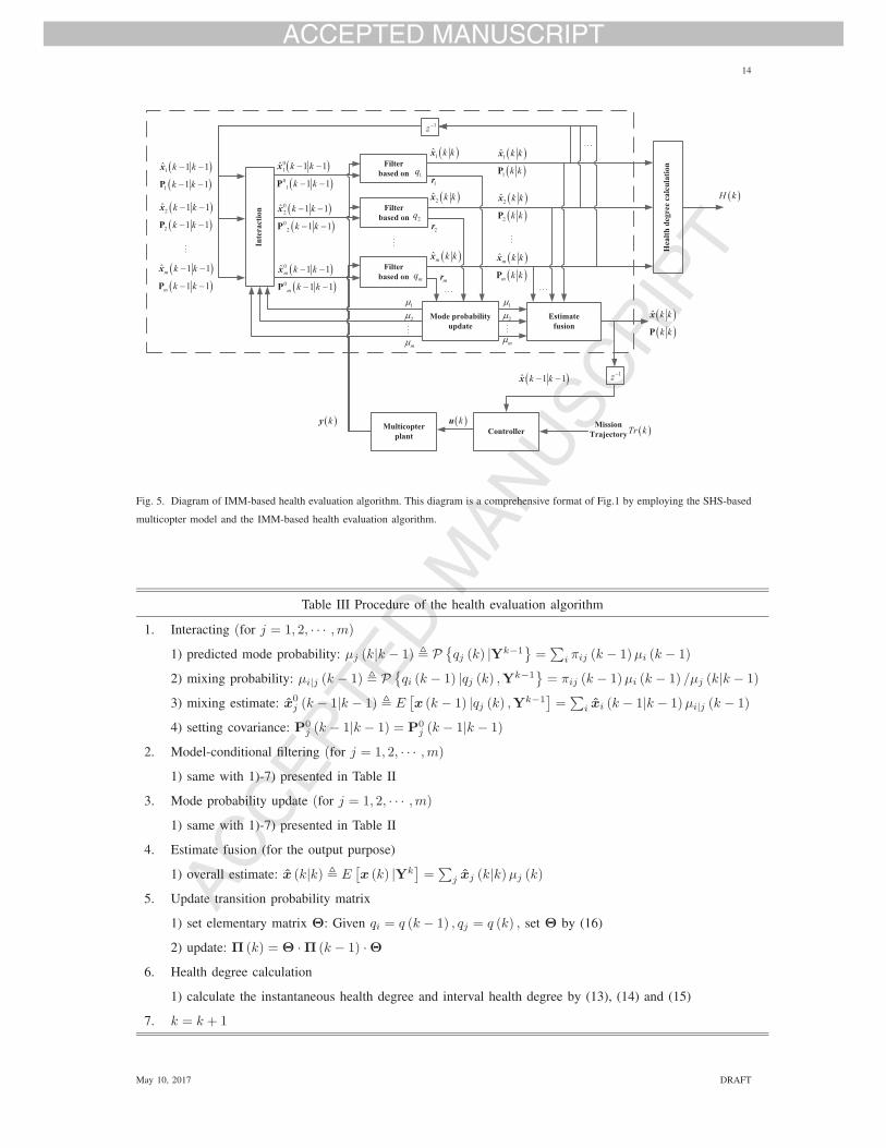
By applying Modifications 1&2 to the classic IMM algorithm, the health evaluation is performed on the

SHS-based multicopter model based on the modified IMM algorithm. The diagram of the health evaluation

process is shown in Fig. 5, and the details of the algorithm are presented in Table III.

May 10, 2017 DRAFT

14

Filterbased on 2q

Filterbased on 1q

Filterbased on mq

Interaction

� �� �

1

1

ˆ 1 1

1 1

k k

k k

� �

� �

x

P

� �� �

2

2

ˆ 1 1

1 1

k k

k k

� �

� �

x

P

� �� �

ˆ 1 1

1 1m

m

k k

k k

� �

� �

x

P

� �� �

01

01

ˆ 1 1

1 1

k k

k k

� �

� �

x

P

� �� �

02

02

ˆ 1 1

1 1

k k

k k

� �

� �

x

P

� �� �

0

0

ˆ 1 1

1 1m

m

k k

k k

� �

� �

x

P

� �� �

1

1

ˆ k k

k k

x

P

� �� �

2

2

ˆ k k

k k

x

P

� �� �

ˆm

m

k k

k k

x

P

� �ky

� �1ˆ k kx

� �2ˆ k kx

� �ˆm k kx

Mode probabilityupdate

Estimatefusion

1r

2r

mr

1

2

m

1

2

m

� �� �ˆ k k

k k

x

P

ControllerMulticopterplant

MissionTrajectory

� �ku� �Tr k

� �ˆ 1 1k k� �x

Healthdegreecalculation

� �H k

1z�

1z�

Fig. 5. Diagram of IMM-based health evaluation algorithm. This diagram is a comprehensive format of Fig.1 by employing the SHS-based

multicopter model and the IMM-based health evaluation algorithm.

Table III Procedure of the health evaluation algorithm

1. Interacting (for j = 1, 2, · · · ,m)

1) predicted mode probability: μj (k|k − 1) � P {qj (k) |Yk−1

}=∑

i πij (k − 1)μi (k − 1)

2) mixing probability: μi|j (k − 1) � P {qi (k − 1) |qj (k) ,Yk−1

}= πij (k − 1)μi (k − 1) /μj (k|k − 1)

3) mixing estimate: x0j (k − 1|k − 1) � E

[x (k − 1) |qj (k) ,Yk−1

]=∑

i xi (k − 1|k − 1)μi|j (k − 1)

4) setting covariance: P0j (k − 1|k − 1) = P0

j (k − 1|k − 1)

2. Model-conditional filtering (for j = 1, 2, · · · ,m)

1) same with 1)-7) presented in Table II

3. Mode probability update (for j = 1, 2, · · · ,m)

1) same with 1)-7) presented in Table II

4. Estimate fusion (for the output purpose)

1) overall estimate: x (k|k) � E[x (k) |Yk

]=∑

j xj (k|k)μj (k)

5. Update transition probability matrix

1) set elementary matrix Θ: Given qi = q (k − 1) , qj = q (k) , set Θ by (16)

2) update: Π (k) = Θ ·Π (k − 1) ·Θ6. Health degree calculation

1) calculate the instantaneous health degree and interval health degree by (13), (14) and (15)

7. k = k + 1

May 10, 2017 DRAFT

15

IV. A CASE STUDY: MULTICOPTER WITH SENSOR ANOMALIES

In this section, the proposed health evaluation method is performed on a multicopter with sensor anomalies.

The sensors GPS, barometer and compass are considered alternately unhealthy in the simulation. The SHS-

based model configuration, simulated flight data generation and health evaluation results are presented. Also,

discussions and some comparisons are given in this section.

A. Model configuration

The parameters in the SHS-based model presented in Section II are listed in Table IV.

Table IV Multicopter model parameters

m 1.535kg

Jx, Jy, Jz 0.0411, 0.0478, 0.0599 kg ·m2

g 9.8 m/s2

T 0.01 s

kP,z, kD,z 10, 8

kP,φ, kD,φ 5, 0.8

kP,θ, kD,θ 5, 0.8

kP,ψ, kD,ψ 5, 0.4

KPa,KDa I2, 2I2

Remark 7. For ease of visualization, the controllers of different health statuses are identical, which will

make readers easy to view the performance deviation from the expected normal condition. Actually, for the

purpose of safety decision-making, the controller of different health statuses should be set to be different. For

example, when the GPS anomaly is detected, the controller should be changed to perform returning home or

landing rather than continue to execute the predetermined mission.

For the system noise w and the noise driven matrix Γw, set

w (·) ∼ N (0,Q)

Γw = diag {0, 0, 0, 1, 1, 1, 0, 0, 0, 1, 1, 1}where

Q = diag {0.01, 0.01, 0.01, 0.01, 0.01, 0.01, 0.001, 0.001, 0.001, 0.001, 0.001, 0.001} .

For measurement noise vj and noise driven matrix Γv,j under each state qj , set

q1 :

⎧⎪⎪⎪⎨⎪⎪⎪⎩

v1 (·) ∼ N (0,R1)

R1 = diag {0.2, 0.2, 0.2, 0.5, 0.5, 0.5, 0.001, 0.001, 0.001, 0.001, 0.001, 0.001}Γv,1 = diag {1, 1, 1, 1, 1, 1, 1, 1, 1, 1, 1, 1}

.

For states q2, q3 and q4, the matrices Rj and Γv,j can be obtained following the principles as presented in

(8)-(10). Referring to [81], [82], [84], [85], the transition probability matrix representing discrete dynamics is

May 10, 2017 DRAFT

16

set as

Π =

⎡⎢⎢⎢⎢⎢⎢⎣

0.97 0.01 0.01 0.01

0.1 0.9 0 0

0.1 0 0.9 0

0.1 0 0 0.9

⎤⎥⎥⎥⎥⎥⎥⎦.

It can be seen that the state q1 is dominant in the configuration of Π. However, the transition probability matrix

will be updated in the modified IMM algorithm. Thus, the restriction that real discrete dynamics should be

precisely known as a priori is relaxed.

B. Simulated flight data generation

Here, equation (7) is used to generate real flight data under different anomalies, including true values of

process variables of the multicopter and their measurements. In the simulation, different anomalies occur

alternately as shown in Table V. The whole simulation time is 160s, and the sample time T = 0.01s.

Table V Simulated flight data generation

Time interval 0-6s 6s-20s 20s-30s

Anomaly type fully healthy GPS measurement with big noise fully healthy

Time interval 30s-40s 40s-50s 50s-60s

Anomaly type barometer measurement with big noise compass measurement with big noise GPS measurement drift

Time interval 60s-70s 70s-90s 90s-100s

Anomaly type fully healthy barometer measurement drift fully healthy

Time interval 100s-130s 130s-160s

Anomaly type barometer measurement lost GPS measurement lost

The observation equation of (7) is used to generate system measurements under the fully healthy status.

For simulating GPS measurement with big noise, the related parameters of covariance matrix R1 of v1 (·) is

temporally increased as

R1 (1, 1) = R1 (2, 2) = 2.2.

For GPS measurement drift, add a random value to the measurements px and py as shown below⎧⎪⎪⎪⎪⎪⎪⎪⎪⎪⎨⎪⎪⎪⎪⎪⎪⎪⎪⎪⎩

y (k) = C1x (k − 1) + Γv,1v1 (k) + Δp (k)

Δp (k) = [Δpx (k) ,Δpy (k) , 0, · · · , 0]T

Δpx (k) = 1 + ξx (k)

Δpy (k) = 2 + ξy (k)

ξx (·) ∼ N (0, 0.1) , ξy (·) ∼ N (0, 0.1)

.

For loss of GPS measurements, (7) is changed to⎧⎨⎩

y1 (k) = y1 (k − 1)

y2 (k) = y2 (k − 1).

For barometer and compass anomalies, similar process is performed to generate related measurements.

May 10, 2017 DRAFT

17

C. Health evaluation results

The proposed health evaluation algorithm is performed on the SHS-based multicopter with the generated flight

data in Table V. The results are shown in Figs. 6-11. According to Definition 2&3, the components {px, py, pz}in x are most concerned in the health evaluation of multicopters. Fig. 6 shows the variation of measurements and

the estimated values of {px, py, pz}. Fig. 7 depicts true values, expected values and estimated values with 95%

confidence interval of {px, py, pz}. Fig. 8 compares the estimation results by using the SHS-based model and

the SCS-based model. From Figs. 6-8, it can be concluded that: 1) despite the incorrect system measurements,

even measurements lost, the process variables x can be also estimated. 2) When sensor anomaly (especially

measurements lost) occurs, the estimated values will deviate from the true values for related components in

x. 3) The estimated values are close to the expected values, because the controller of the multicopter always

“thinks” that it makes the multicopter fly along the expected trajectory, despite the true trajectory deviates. 4)

By using the modified IMM algorithm, both the estimate values of x and the covariance matrix are obtained.

Thus, a 95% confidence interval is displayed in Fig. 7, which covers the true trajectory of the multicopter.

Note that when the estimate values of x are precise, the confidence interval is narrow, which cannot be clearly

depicted. 5) Compared with the estimation results with the SCS-based model, system variables can be estimated

with smaller errors in a short time horizon with the SHS-based model after anomaly happens. It means that the

SHS-based model is better and more robust than a single dynamic model for the purpose of health evaluation.

0 20 40 60 80 100 120 140 160-10

0

10

20

time/s

p x

0 20 40 60 80 100 120 140 160-10

0

10

20

time/s

p y

0 20 40 60 80 100 120 140 160-10

0

10

20

time/s

p z

measured estimated

Fig. 6. Measurements and estimates of {px, py , pz} .

Figs. 9&10 present the probabilities of different health statuses and state identification results based on the

modified IMM algorithm, and the performance is compared with the classic IMM algorithm. The result shows

that by updating the transition probability matrix, the modified IMM algorithm performs better than the classic

May 10, 2017 DRAFT

18

true expected

estimated 95% confidence interval

(a) (b)

time/s

p x

Whole time interval [0,160]

20 40 60 80 100 120 140 160

-5

0

5

10

time/s

p y

20 40 60 80 100 120 140 160

-5

0

5

10

time/s

p z

20 40 60 80 100 120 140 1600

5

10

15

time/s

p x

A local view of time interval [120,160]

120 130 140 150 160

5

10

15

time/s

p y

120 130 140 150 160

5

10

15

time/s

p z

120 130 140 150 1600

5

10

15

Fig. 7. True values, expected values, and estimates with 95% confidence interval of {px, py , pz}.

one. After obtaining the pdf f(x (k)

∣∣qj (k) ,Yk)

and the probability P (q (k)

∣∣Yk)

of (13) as shown in Figs.

7&9, the health degree can be calculated according to (14) and (15). Here, the tolerant threshold ε in Definition

2&3 is set to 0.3m. The instantaneous health degree is calculated for each sample time T , and the interval

health degree is calculated for every 5 seconds interval. The result is shown in Fig. 11. From Fig. 11, it can

be seen that the health degree will decrease when sensor anomalies occurs, which proves the variation of

health degree is able to reflect system anomalies and performance degradation. Here, two comparative health

evaluation results are also presented. 1) As shown in Fig. 8, the distribution of process variables can be also

obtained by EKF based on the SCS-based model. On this basis, the health degree is calculated and depicted in

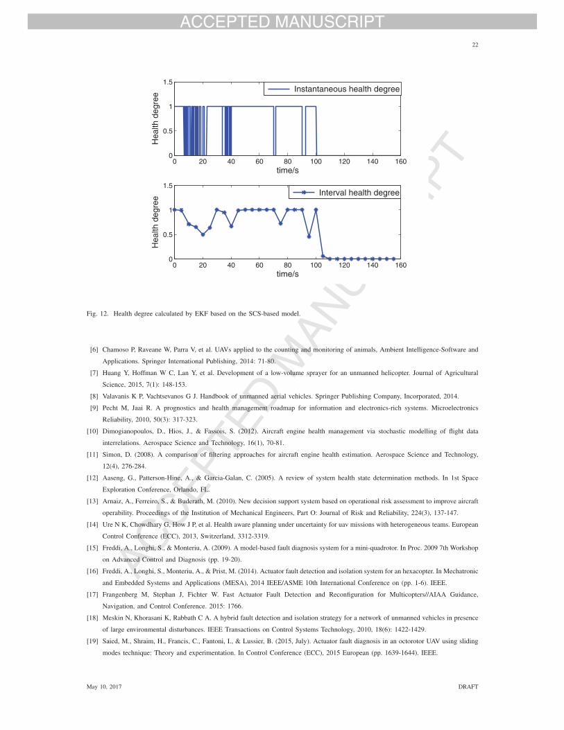
Fig. 12. Comparing Fig. 11 with Fig. 12, it indicates that the health degree calculated by the modified IMM

algorithm and the SHS-based model is more accurate than that calculated by EKF and the SCS-based model.

This is because the distribution of process variables estimated by the modified IMM algorithm is more accurate

than that estimated by EKF, which has been shown in Fig. 8. 2) Fig. 6 shows the estimate of {px, py, pz}.

Existed research usually gets the health information of a dynamical system by comparing the estimated value of

process variables with a health set. If the values of process variables at a time index or over a time interval are

in the range of the health set, the system is considered healthy (the health degree is 1); otherwise, the system is

May 10, 2017 DRAFT

19

0 50 100 150-20

0

20

time/sp x

SHS-based Model

0 50 100 150-20

0

20

time/s

p y

0 50 100 150-20

0

20

time/s

p z0 50 100 150

-2000

0

2000

time/s

p x

SCS-based Model

0 50 100 150-20

0

20

time/s

p y

0 50 100 150-500

0

500

time/sp z

true estimated(a) (b)

Fig. 8. Process variable estimation based on the SHS-based model and the SCS-based model.

considered unhealthy (the health degree is 0). Following this principle, the estimated values of {px, py, pz} are

compared to the health set, and the result is shown in Fig. 13. Comparing Fig. 11 with Fig. 13, it reflects that the

health degree is more sensitive to anomalies than the health evaluation result merely obtained by a comparison

between system process variables and the health set. This is because the definition of health degree introduces

the probability measure to health evaluation by considering uncertainties, which is more appropriate for health

evaluation of dynamical systems. As to the practical application of the proposed method, since the IMM-based

algorithm is based on filtering techniques, it is easy to implement the whole algorithm in practical engineering.

As to the instantaneity, the presented case study is simulated by MATLAB R2010b on a desktop. The average

operating time of each cycle is less than 1ms, meaning that compared to the sample time T = 0.01s, the

proposed health evaluation method is able to satisfy the instantaneity requirement.

V. CONCLUSION

This paper proposes a health evaluation method of multicopters. The multicopter is modeled by SHS, and its

health is quantitatively measured by introducing a definition of health degree. Then, a modified IMM algorithm

is proposed to estimate real-time hybrid state distribution. On this basis, the health degree is calculated. A case

study of multicopter with sensor anomalies is presented to validate the effectiveness of the proposed method. The

advantages of the SHS-based multicopter modeling and the health evaluation method presented in this paper are

summarized in three aspects: 1) the SHS-based modeling concerns the safety issue of multicopters. The discrete

and continuous dynamics in SHS can model different health statuses and corresponding dynamic behaviors. The

simulation results show that the performance of the SHS-based model behaves better than the SCS-based model.

May 10, 2017 DRAFT

20

0 20 40 60 80 100 120 140 1600

0.2

0.4

0.6

0.8

1

time/s

prob

abili

ty

The modified IMM algorithm

0 20 40 60 80 100 120 140 1600

0.2

0.4

0.6

0.8

1

time/s

prob

abili

ty

The classic IMM algorithm

q1 q2 q3 q4(a) (b)

Fig. 9. Health status probability obtained by the modified IMM algorithm and the classic IMM algorithm.

0 20 40 60 80 100 120 140 1600

0.5

1

1.5

2

2.5

3

3.5

4

time/s

Mod

e

The modified IMM algorithm

trueestimated

0 20 40 60 80 100 120 140 1600

0.5

1

1.5

2

2.5

3

3.5

4

time/s

Mod

e

The classic IMM algorithm

trueestimated

(a) (b)

Fig. 10. Health status identification result obtained by the modified IMM algorithm and the classic IMM algorithm.

2) The health degree introduced in this paper gives a quantitative indicator of system performance, which is

beneficial to pilots for understanding the working condition of multicopters. 3) The modified IMM algorithm

outputs the multivariate Gaussian distribution of system process variables rather than just the estimated values,

which provides more useful information about multicopter performance, especially when anomaly occurs. In

future research, the proposed method can be extended in three aspects: 1) other anomalies such as propulsion

system anomaly and communication breakdown can be added into the SHS-based multicopter model to extend

May 10, 2017 DRAFT

21

0 20 40 60 80 100 120 140 1600

0.5

1

1.5

time/s

Hea

lth d

egre

e

Instantaneous health degree

0 20 40 60 80 100 120 140 1600

0.5

1

1.5

time/s

Hea

lth d

egre

e

Interval health degree

Fig. 11. Health degree calculated by the modified IMM algorithm based on the SHS-based model.

the applicability of the proposed method. 2) Since the health degree is calculated on the system process variables,

the health evaluation result is sensitive to external disturbances, which bring fluctuations to process variables.

In order to solve this problem, the wind model should be added in the SHS-based multicopter model, or a

health evaluation algorithm of a homogeneous multicopter team should be established. The two manners can

effectively evaluate the amplitude and form of the external disturbance, and eliminate its influence on health

degree calculation. 3) After health evaluation, health prediction and management is the next procedures of the

PHM system as shown in Fig. 1. The concept of stochastic reachability has been already presented to predict

system behavior in SHS research [41], [90]. Combining the health prediction and stochastic reachability to

extend the current work is an emphasis of future research. As to the management level, a multicopter failsafe

mechanism dealt with multiple failures will be also established based on health evaluation results in future

research.

REFERENCES

[1] Tomic T, Schmid K, Lutz P, et al. Toward a fully autonomous UAV: Research platform for indoor and outdoor urban search and

rescue. IEEE robotics & automation magazine, 2012, 19(3): 46-56.

[2] Goodrich M A, Morse B S, Gerhardt D, et al. Supporting wilderness search and rescue using a camera-equipped mini UAV. Journal

of Field Robotics, 2008, 25(1-2): 89-110.

[3] Agha-mohammadi A, Ure N K, How J P, et al. Health aware stochastic planning for persistent package delivery missions using

quadrotors//2014 IEEE/RSJ International Conference on Intelligent Robots and Systems. IEEE, 2014: 3389-3396.

[4] Girard A R, Howell A S, Hedrick J K. Border patrol and surveillance missions using multiple unmanned air vehicles//Decision and

Control, 2004. CDC. 43rd IEEE Conference on. IEEE, 2004, 1: 620-625.

[5] Bethke B, How J P, Vian J. Multi-UAV persistent surveillance with communication constraints and health management//AIAA

Guidance, Navigation, and Control Conference (GNC). 2009.

May 10, 2017 DRAFT

22

0 20 40 60 80 100 120 140 1600

0.5

1

1.5

time/s

Hea

lth d

egre

e

Instantaneous health degree

0 20 40 60 80 100 120 140 1600

0.5

1

1.5

time/s

Hea

lth d

egre

e

Interval health degree

Fig. 12. Health degree calculated by EKF based on the SCS-based model.

[6] Chamoso P, Raveane W, Parra V, et al. UAVs applied to the counting and monitoring of animals, Ambient Intelligence-Software and

Applications. Springer International Publishing, 2014: 71-80.

[7] Huang Y, Hoffman W C, Lan Y, et al. Development of a low-volume sprayer for an unmanned helicopter. Journal of Agricultural

Science, 2015, 7(1): 148-153.

[8] Valavanis K P, Vachtsevanos G J. Handbook of unmanned aerial vehicles. Springer Publishing Company, Incorporated, 2014.

[9] Pecht M, Jaai R. A prognostics and health management roadmap for information and electronics-rich systems. Microelectronics

Reliability, 2010, 50(3): 317-323.

[10] Dimogianopoulos, D., Hios, J., & Fassois, S. (2012). Aircraft engine health management via stochastic modelling of flight data

interrelations. Aerospace Science and Technology, 16(1), 70-81.

[11] Simon, D. (2008). A comparison of filtering approaches for aircraft engine health estimation. Aerospace Science and Technology,

12(4), 276-284.

[12] Aaseng, G., Patterson-Hine, A., & Garcia-Galan, C. (2005). A review of system health state determination methods. In 1st Space

Exploration Conference, Orlando, FL.

[13] Arnaiz, A., Ferreiro, S., & Buderath, M. (2010). New decision support system based on operational risk assessment to improve aircraft

operability. Proceedings of the Institution of Mechanical Engineers, Part O: Journal of Risk and Reliability, 224(3), 137-147.

[14] Ure N K, Chowdhary G, How J P, et al. Health aware planning under uncertainty for uav missions with heterogeneous teams. European

Control Conference (ECC), 2013, Switzerland, 3312-3319.

[15] Freddi, A., Longhi, S., & Monteriu, A. (2009). A model-based fault diagnosis system for a mini-quadrotor. In Proc. 2009 7th Workshop

on Advanced Control and Diagnosis (pp. 19-20).

[16] Freddi, A., Longhi, S., Monteriu, A., & Prist, M. (2014). Actuator fault detection and isolation system for an hexacopter. In Mechatronic

and Embedded Systems and Applications (MESA), 2014 IEEE/ASME 10th International Conference on (pp. 1-6). IEEE.

[17] Frangenberg M, Stephan J, Fichter W. Fast Actuator Fault Detection and Reconfiguration for Multicopters//AIAA Guidance,

Navigation, and Control Conference. 2015: 1766.

[18] Meskin N, Khorasani K, Rabbath C A. A hybrid fault detection and isolation strategy for a network of unmanned vehicles in presence

of large environmental disturbances. IEEE Transactions on Control Systems Technology, 2010, 18(6): 1422-1429.

[19] Saied, M., Shraim, H., Francis, C., Fantoni, I., & Lussier, B. (2015, July). Actuator fault diagnosis in an octorotor UAV using sliding

modes technique: Theory and experimentation. In Control Conference (ECC), 2015 European (pp. 1639-1644). IEEE.

May 10, 2017 DRAFT

23

0 20 40 60 80 100 120 140 1600

0.5

1

1.5

time/s

Hea

lth d

egre

e

Instantaneous health degree

0 20 40 60 80 100 120 140 1600

0.5

1

1.5

time/s

Hea

lth d

egre

e

Interval health degree

Fig. 13. Health evaluation calculated by a comparison between system process variables and the health set.

[20] Blanke, M., Staroswiecki, M., & Wu, N. E. (2001). Concepts and methods in fault-tolerant control. In American Control Conference,

2001. Proceedings of the 2001 (Vol. 4, pp. 2606-2620). IEEE.

[21] Falconi G P, Holzapfel F. Adaptive fault tolerant control allocation for a hexacopter system//American Control Conference (ACC),

2016. American Automatic Control Council (AACC), 2016: 6760-6766.

[22] Dydek Z T, Annaswamy A M, Lavretsky E. Adaptive control of quadrotor UAVs: A design trade study with flight evaluations. IEEE

Transactions on control systems technology, 2013, 21(4): 1400-1406.

[23] Zhang Y, Jiang J. Integrated design of reconfigurable fault-tolerant control systems. Journal of Guidance, Control, and Dynamics,

2001, 24(1): 133-136.

[24] Raabe, C. T., & Suzuki, S. (2013). Adaptive failure-tolerant control for hexacopters. In AIAA Infotech@ Aerospace Conference, ser.

Guidance, Navigation, and Control and Co-located Conferences. American Institute of Aeronautics and Astronautics.

[25] Gao, C., & Duan, G. (2014). Fault diagnosis and fault tolerant control for nonlinear satellite attitude control systems. Aerospace

Science and Technology, 33(1), 9-15.

[26] Sheppard, J. W., Kaufman, M., & Wilmer, T. J. (2009). IEEE standards for prognostics and health management. Aerospace and

Electronic Systems Magazine, IEEE, 24(9), 34-41.

[27] Venkatasubramanian, V., Rengaswamy, R., Yin, K., & Kavuri, S. N. (2003). A review of process fault detection and diagnosis: Part

I: Quantitative model-based methods. Computers & chemical engineering, 27(3), 293-311.

[28] Gao Z, Cecati C, Ding S X. A survey of fault diagnosis and fault-tolerant techniques-Part I: fault diagnosis With model-based and

signal-based approaches. IEEE Transactions on Industrial Electronics, 2015, 62(6): 3757-3767.

[29] Wang G, Huang Z. Data-driven fault-tolerant control design for wind turbines with robust residual generator. IET Control Theory &

Applications, 2015, 9(7): 1173-1179.

[30] Sun, Z., Qin, S. J., Singhal, A., & Megan, L. (2012, June). Control performance monitoring via model residual assessment. In

American Control Conference (ACC), 2012 (pp. 2800-2805). IEEE.

[31] Bai, G., Wang, P., & Hu, C. (2015). A self-cognizant dynamic system approach for prognostics and health management. Journal of

Power Sources, 278, 163-174.

[32] Zio, E., & Di Maio, F. (2010). A data-driven fuzzy approach for predicting the remaining useful life in dynamic failure scenarios of

a nuclear system. Reliability Engineering & System Safety, 95(1), 49-57.

[33] Feng, Z., Liang, M., & Chu, F. (2013). Recent advances in time-frequency analysis methods for machinery fault diagnosis: A review

May 10, 2017 DRAFT

24

with application examples. Mechanical Systems and Signal Processing, 38(1), 165-205.

[34] Henriquez, P., Alonso, J. B., Ferrer, M., & Travieso, C. M. (2014). Review of automatic fault diagnosis systems using audio and

vibration signals. Systems, Man, and Cybernetics: Systems, IEEE Transactions on, 44(5), 642-652.

[35] Lu, H., Kolarik, W. J., & Lu, H. (2001). Real-time performance reliability prediction. Reliability, IEEE Transactions on, 50(4),

353-357.

[36] Cai, K., Introduction to Fuzzy Reliability. NewYork,NY,USA: Kluwer Academic Publishers, 1996.

[37] Xu, Z., Ji, Y., & Zhou, D. (2009). A new real-time reliability prediction method for dynamic systems based on on-line fault prediction.

Reliability, IEEE Transactions on, 58(3), 523-538.

[38] Zhao Z, Quan Q, Cai K Y. A profust reliability based approach to prognostics and health management. IEEE Transactions on

Reliability, 2014, 63(1): 26-41.

[39] Koutsoukos, X. D., & Riley, D. (2008). Computational methods for verification of stochastic hybrid systems. Systems, Man and

Cybernetics, Part A: Systems and Humans, IEEE Transactions on, 38(2), 385-396.

[40] Abate, A., Katoen, J. P., Lygeros, J., & Prandini, M. (2010). Approximate model checking of stochastic hybrid systems. European

Journal of Control, 16(6), 624-641.

[41] Abate, A., Prandini, M., Lygeros, J., & Sastry, S. (2008). Probabilistic reachability and safety for controlled discrete time stochastic

hybrid systems. Automatica, 44(11), 2724-2734.

[42] Liu, W., & Hwang, I. (2012, June). A stochastic approximation based state estimation algorithm for stochastic hybrid systems. In

American Control Conference (ACC), 2012 (pp. 312-317). IEEE.

[43] Liu, W., & Hwang, I. (2014). On hybrid state estimation for stochastic hybrid systems. Automatic Control, IEEE Transactions on,

59(10), 2615-2628.

[44] Discalea F L, Matt H, Bartoli I, et al. Health monitoring of UAV wing skin-to-spar joints using guided waves and macro fiber

composite transducers. Journal of intelligent material systems and structures, 2007, 18(4): 373-388.

[45] Oliver J A, Kosmatka J B, Farrar C R, et al. Development of a composite UAV wing test-bed for structural health monitoring

research//The 14th International Symposium on: Smart Structures and Materials & Nondestructive Evaluation and Health Monitoring.

International Society for Optics and Photonics, 2007.

[46] Jiang Y, Zhiyao Z, Haoxiang L, et al. Fault detection and identification for quadrotor based on airframe vibration signals: A data-driven

method//Control Conference (CCC), 2015 34th Chinese. IEEE, 2015: 6356-6361.

[47] Kressel I, Handelman A, Botsev Y, et al. Evaluation of flight data from an airworthy structural health monitoring system integrally

embedded in an unmanned air vehicle//6th European Workshop on Structural Health Monitoring. 2012: 193-200.

[48] Kressel I, Balter J, Mashiach N, et al. High speed, in-flight structural health monitoring system for medium altitude long endurance

unmanned air vehicle//EWSHM-7th European Workshop on Structural Health Monitoring. 2014.

[49] Cen, Z., Noura, H., & Al Younes, Y. (2013). Robust fault estimation on a real quadrotor UAV using optimized adaptive Thau observer.

In Unmanned Aircraft Systems (ICUAS), 2013 International Conference on (pp. 550-556). IEEE.

[50] Lu, P., Van Kampen, E. J., & Yu, B. (2014). Actuator fault detection and diagnosis for quadrotors. In IMAV 2014: International

Micro Air Vehicle Conference and Competition 2014, Delft, The Netherlands, August 12-15, 2014. Delft University of Technology.

[51] Garcia D, Moncayo H, Perez A, et al. Low cost implementation of a biomimetic approach for UAV health management//American

Control Conference (ACC), 2016. IEEE, 2016: 2265-2270.

[52] Du G X, Quan Q, Yang B, et al. Controllability analysis for multirotor helicopter rotor degradation and failure. Journal of Guidance,

Control, and Dynamics, 2015, 38(5): 978-985.

[53] Heredia G, Ollero A, Bejar M, et al. Sensor and actuator fault detection in small autonomous helicopters. Mechatronics, 2008, 18(2):

90-99.

[54] Lu P, van Kampen E J, de Visser C, et al. Nonlinear aircraft sensor fault reconstruction in the presence of disturbances validated by

real flight data. Control Engineering Practice, 2016, 49: 112-128.

[55] Ansari A, Bernstein D S. Aircraft sensor fault detection using state and input estimation//American Control Conference (ACC), 2016.

IEEE, 2016: 5951-5956.

[56] Yun-hong G, Ding Z, Yi-bo L. Small UAV sensor fault detection and signal reconstruction//Mechatronic Sciences, Electric Engineering

and Computer (MEC), Proceedings 2013 International Conference on. IEEE, 2013: 3055-3058.

[57] Rudin K, Ducard G J J, Siegwart R Y. A sensor fault detection for aircraft using a single Kalman filter and hidden Markov models//2014

IEEE Conference on Control Applications (CCA). IEEE, 2014: 991-996.

[58] Abbaspour A, Aboutalebi P, Yen K K, et al. Neural adaptive observer-based sensor and actuator fault detection in nonlinear systems:

Application in UAV. ISA transactions, 2016.

May 10, 2017 DRAFT

25

[59] Lopez-Estrada F R, Ponsart J C, Theilliol D, et al. Robust sensor fault diagnosis and tracking controller for a UAV modelled as LPV

system//Unmanned Aircraft Systems (ICUAS), 2014 International Conference on. IEEE, 2014: 1311-1316.

[60] Caliskan F, Hajiyev C. Active fault-tolerant control of UAV dynamics against sensor-actuator failures. Journal of Aerospace

Engineering, 2016.

[61] Jeong J, Son Y, Jung J, et al. An election scheme for cooperative UAVs with fault tolerance. Advanced Science and Technology

Letters, 2015, 110: 79-82.

[62] Birnbaum Z, Dolgikh A, Skormin V, et al. Unmanned aerial vehicle security using behavioral profiling//Unmanned Aircraft Systems

(ICUAS), 2015 International Conference on. IEEE, 2015: 1310-1319.

[63] Bhattacharya S, Basar T. Game-theoretic analysis of an aerial jamming attack on a UAV communication network//Proceedings of the

2010 American Control Conference. IEEE, 2010: 818-823.

[64] Bhattacharya S. Differential game-theoretic approach for spatial jamming attack in a UAV communication network//In 14th

International Symposium on Dynamic Games and Applications. 2010.

[65] Kim J, Cho B H. State-of-charge estimation and state-of-health prediction of a Li-ion degraded battery based on an EKF combined

with a per-unit system. IEEE Transactions on Vehicular Technology, 2011, 60(9): 4249-4260.

[66] Barre A, Deguilhem B, Grolleau S, et al. A review on lithium-ion battery ageing mechanisms and estimations for automotive

applications. Journal of Power Sources, 2013, 241: 680-689.

[67] Charkhgard M, Farrokhi M. State-of-charge estimation for lithium-ion batteries using neural networks and EKF. IEEE transactions

on industrial electronics, 2010, 57(12): 4178-4187.

[68] Sepasi S, Ghorbani R, Liaw B Y. Improved extended Kalman filter for state of charge estimation of battery pack. Journal of Power

Sources, 2014, 255: 368-376.

[69] Zhang J, Lee J. A review on prognostics and health monitoring of Li-ion battery. Journal of Power Sources, 2011, 196(15): 6007-6014.

[70] Goebel K, Saha B, Saxena A, et al. Prognostics in battery health management. IEEE instrumentation & measurement magazine, 2008,

11(4): 33.

[71] Rahimi-Eichi H, Ojha U, Baronti F, et al. Battery management system: an overview of its application in the smart grid and electric

vehicles. IEEE Industrial Electronics Magazine, 2013, 7(2): 4-16.

[72] Saha B, Koshimoto E, Quach C C, et al. Battery health management system for electric UAVs//Aerospace Conference, 2011 IEEE,

2011: 1-9.

[73] Bethke B, How J P, Vian J. Group health management of UAV teams with applications to persistent surveillance//2008 American

Control Conference. IEEE, 2008: 3145-3150.

[74] Valenti M, Bethke B, How J P, et al. Embedding health management into mission tasking for UAV teams//American control conference.

2007: 5777-5783.

[75] Izadi, H. A., Zhang, Y., & Gordon, B. W. (2011). Fault tolerant model predictive control of quad-rotor helicopters with actuator fault

estimation. In Proceedings of the 18th IFAC World Congress (Vol. 18, No. 1, pp. 6343-6348).

[76] Sadeghzadeh, I., & Zhang, Y. M. (2011). A review on fault-tolerant control for unmanned aerial vehicles (UAVs). Infotech@ Aerospace,

St. Louis, MO.

[77] Chamseddine, A., Theilliol, D., Zhang, Y. M., Join, C., & Rabbath, C. A. (2015). Active fault-tolerant control system design with

trajectory re-planning against actuator faults and saturation: Application to a quadrotor unmanned aerial vehicle. International Journal

of Adaptive Control and Signal Processing, 29(1), 1-23.

[78] Braun, M., & Golubitsky, M. (1983). Differential equations and their applications (pp. 343-350). New York: Springer.

[79] Vichare, N. M., & Pecht, M. G. (2006). Prognostics and health management of electronics. Components and Packaging Technologies,

IEEE Transactions on, 29(1), 222-229.

[80] Beigi, H., Betti, R., & Balsamo, L. (2014). U.S. Patent Application No. 14/297,595.

[81] Zhang, Y., & Li, X. R. (1998). Detection and diagnosis of sensor and actuator failures using IMM estimator. Aerospace and Electronic

Systems, IEEE Transactions on, 34(4), 1293-1313.

[82] Zhao, S., Huang, B., & Liu, F. (2015). Fault detection and diagnosis of multiple-model systems with mismodeled transition

probabilities. Industrial Electronics, IEEE Transactions on, 62(8), 5063-5071.

[83] Zhou, Y., Wang, D., Huang, H., Li, J., & Yi, L. (2011). Fuzzy logic based interactive multiple model fault diagnosis for PEM fuel

cell systems. INTECH Open Access Publisher.

[84] Compare, M., Baraldi, P., Turati, P., & Zio, E. (2015). Interacting multiple-models, state augmented particle filtering for fault

diagnostics. Probabilistic Engineering Mechanics, 40, 12-24.

May 10, 2017 DRAFT

26

[85] Tudoroiu, N., Sobhani-Tehrani, E., & Khorasani, K. (2006). Interactive bank of unscented Kalman filters for fault detection and

isolation in reaction wheel actuators of satellite attitude control system. In IEEE Industrial Electronics, IECON 2006-32nd Annual

Conference on (pp. 264-269). IEEE.

[86] Jeon, D., & Eun, Y. (2014). Distributed asynchronous multiple sensor fusion with nonlinear multiple models. Aerospace Science and

Technology, 39, 692-704.

[87] Jilkov, V. P., & Li, X. R. (2004). Online Bayesian estimation of transition probabilities for Markovian jump systems. Signal Processing,

IEEE Transactions on, 52(6), 1620-1630.

[88] Seah, C. E., & Hwang, I. (2009). Stochastic linear hybrid systems: Modeling, estimation, and application in air traffic control. Control

Systems Technology, IEEE Transactions on, 17(3), 563-575.

[89] Blom, H. A., & Bar-Shalom, Y. (1988). The interacting multiple model algorithm for systems with Markovian switching coefficients.

Automatic Control, IEEE Transactions on, 33(8), 780-783.

[90] Bujorianu, L. M. (2012). Applications of stochastic reachability. In Stochastic Reachability Analysis of Hybrid Systems (pp. 203-207).

Springer London.

May 10, 2017 DRAFT

本文献由“学霸图书馆-文献云下载”收集自网络，仅供学习交流使用。

学霸图书馆（www.xuebalib.com）是一个“整合众多图书馆数据库资源，

提供一站式文献检索和下载服务”的24 小时在线不限IP

图书馆。

图书馆致力于便利、促进学习与科研，提供最强文献下载服务。

图书馆导航：

图书馆首页 文献云下载 图书馆入口 外文数据库大全 疑难文献辅助工具