ORIGINAL ARTICLE

A high-accuracy trajectory following controllerfor pneumatic devices

J. Falcão Carneiro & F. Gomes de Almeida

Received: 30 June 2011 /Accepted: 10 October 2011# Springer-Verlag London Limited 2011

Abstract The use of pneumatic devices is widespreadamong different industrial fields, in tasks like handling orassembly. Pneumatic systems are low-cost, reliable, andcompact solutions. However, its use is typically restricted tosimple tasks due to the poor performance achieved inapplications where accurate motion control is required. Thispaper presents a novel nonlinear controller, using neuralnetwork-based models, that allows the use of commonindustrial servopneumatic components in applicationswhere fine trajectory following tasks is required. Furthermore,several experimental trials show that the system is highlyrobust to payload variation without any controller retuning.These results encourage the use of pneumatics actuators in aset of applications for which they have not been traditionallyconsidered.

Keywords Servopneumatic systems . Trajectory followingindustrial tasks . Artificial neural networks . Nonlinearcontrol

1 Introduction

Pneumatic devices are inexpensive, clean, do not overheat,do not produce magnetic fields, and present a high power toweight ratio. Furthermore, pneumatic energy is readilyavailable in most manufacturing facilities. Despite thesefacts, pneumatic systems are seldom used in applicationswhere fine motion control is needed, like for example

welding, robotic manipulation, or fluid injection. This iscaused by the highly nonlinear behavior of pneumatic systemsthat makes them very difficult to model and control. Theevolution in computer processing of recent decades endorsedthe possibility of applying highly evolved nonlinear controland modeling techniques to servopneumatics. This factoralong with the appearance of certain applications for whichpneumatic systems are a natural choice gave rise to a refreshedinterest of researchers around the world on this subject. Forinstance, in [1], Kagawa et al. describe an application wherethe fast and fine positioning of semiconductor wafers mustbe obtained in an environment without electromagnetic fieldsor excessive heat generation. These requirements arenaturally fulfilled by pneumatic actuators.

There are several challenging problems in servopneumaticsystemsmodeling. For instance, the model of a servovalve canbe developed to be used in valve design and onlinemonitoringof valve operating conditions [2] or more dedicated to controlpurposes [3–6]. Regarding the mechanical model, friction isperhaps the most challenging task. The control engineer isusually faced with a difficult tradeoff: how to balance thesimplicity required to synthesize the control law whilemaintaining the complexity necessary for a realistic frictiondescription. Several studies in literature can be found,ranging from the simple, static, Karnopp friction model [7],to the more complex, dynamic, Lugre model [8] and itsevolutions [9].

The model of each pneumatic chamber can be obtainedusing thermodynamic laws and is a second-order modelwith temperature and pressure as state variables [10]. Thismodel is usually simplified by neglecting the temperaturedynamics and considering a polytropic process. Guidelineson which reduced order model to use can be found in [11].It is also possible to find in literature studies with a highlevel of detail in mechanical modeling. For instance, the

J. F. Carneiro (*) : F. G. de AlmeidaIDMEC, Faculdade de Engenharia, Universidade do Porto,Rua Dr. Roberto Frias, s/n,4200-465, Porto, Portugale-mail: jpbrfc@fe.up.pt

Int J Adv Manuf TechnolDOI 10.1007/s00170-011-3695-6

model developed in [12] accounts for the end of strokecylinder cushioning and the model developed in [10]accounts for the connecting tube pressure dynamics.

Very different control strategies, ranging from classical PID[13] to fuzzy logic [14], are used to handle servopneumaticsystems challenges. One of the most used control strategiesis state feedback. It is possible to find studies using linearstate feedback since the 1980s ([15, 16]) up until morerecently [17]. Nonlinear state feedback techniques [18, 19]have also been applied to servopneumatics for instance byRichard and Scavarda in [3] and, more recently, by Richardand Outbib [20]. This technique can also be found in a recentstudy by Xiang and Wikander [21] where excellentexperimental results are reported in positioning tasks.Despite this fact, it is not possible to find in [21] eithertrajectory following results or robustness tests to parametricchanges. Other interesting control techniques also applied toservopneumatics are gain scheduling techniques [22, 23] andadaptive control [24–27].

In order to cope with the high uncertainty of pneumaticsystem modeling, several studies use variable structurecontrollers (VSC) [19]. For instance, Drakunov et al. [28]developed an interesting control architecture that integratesdifferent techniques for the mechanical and the pressuredynamics: a VSC controller is used for the pressuredynamics and a nonlinear state feedback is used for themechanical dynamics. Other studies using VSC controllerswhere developed by Pandian et al. in [29] and by Richerand Hurmuzlu in [30]. It is also possible to findapplications of high-order sliding mode controllers [31] inpneumatics, for example in the study developed by Smaouiet al. in [32].

Another approach that has been tested in servopneumaticsystems is the use of artificial neural networks (ANN) andfuzzy logic-based control [14]. For instance, in [33], Junboet al. developed a controller that is an online-trained three-layer ANN with a non-conventional training algorithm alsodeveloped in [33]. This study has also an interestingparticularity: the valves attached to the cylinder areproportional pressure-reducing valves. In a more recentstudy, Lee et al. [34] use ANN to compensate frictioneffects, in a similar way to the one followed in the presentwork. Sinusoidal position references with different amplitudes(30 to 70mm) and frequencies (0.1 and 0.5 Hz) are used to testthe performance of the controlled system. The maximumtracking error is found to be between 6 and 16 mm.

The costs associated with servovalves can be reduced byusing less expensive ON/OFF valves [23]. In [35] thisapproach was applied to a pneumatic system comprising adouble-acting cylinder and two ON/OFF valves with 5 msswitching time. The control law is a PID with frictioncompensation. The reported experimental results are veryinteresting since that even with a sixfold mass variation the

trajectory following error is below 2 mm. In another work[36], one of the strategies proposed in [35] is enhanced andtested in a vertically mounted pneumatic actuator. Althoughfaster valves are used in [36] (2 ms switching time), resultsare worse than those obtained in [35], namely a maximumerror of about 4 mm when following a ramp reference.

In most of the above described studies the errors intrajectory following tasks are of a few millimeters andheavily depend on the load. In the present work, aninnovative servopneumatic device is presented that canachieve an error below 1 mm, without any controllerretuning, when following variable frequency sinusoids withloads ranging from 2.69 to 13.1 kg.

This paper is organized as follows. In Section 2 theexperimental setup is described and its complete modelpresented. Section 3 is dedicated to the presentation of aninnovative nonlinear controller which is subsequently testedin Section 4. Finally, Section 5 discusses the mainconclusions drawn from this work.

2 Servopneumatic system

2.1 Experimental setup

The experimental setup used in this work includes twosubsystems: (1) the data acquisition and control hardware/software and (2) the electropneumatic components. The dataacquisition and control system comprises a PC with dataacquisition boards and all the hardware/software needed forsignal conditioning. The electropneumatic system presentedin Fig. 1 includes an air treatment unit, two servovalves, apneumatic actuator driving the carriage of a monorailguideway, two pressure transducers, an accelerometer and a

Actuator

Servovalves

Air treatment unit

Carriage

Fig. 1 Experimental setup

Int J Adv Manuf Technol

position encoder integrated in the guidance system. Theencoder is manufactured by Rexroth, has a resolution of5 μm and an accuracy of ±30 μm. The pneumatic actuator ismanufactured by Asco-Joucomatic and has a stroke length of400 mm, a piston diameter ϕ=32 mm and a rod diameterϕh=16 mm. Both servovalves are manufactured by Festo(MPYE-5-1/8-HF-010-B), are used as three-orifice valvesand have a nominal mass flow of 700 slpm. Table 1 resumesthe main system parameters.

2.2 System model

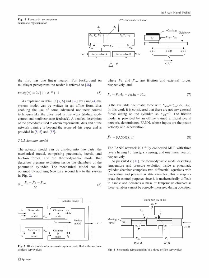
Figure 2 presents a schematic representation of thepneumatic servosystem where P, T, V, and A representpressure, temperature, volume, and area of each chamber,respectively. The moving mass M can be changed from2.69 to 13.1 kg and the source pressure Ps is set at Ps=7 bar. The mass of air flowing into/from each chamber( �mA and �mB) is modulated by two servovalves A and B byvarying the control action uA and uB, respectively. Noticethat although the use of a single five-orifice servovalve ismore common in pneumatic literature (see for instance [10,28, 30]), considering two servovalves allows an extradegree of freedom that can be exploited to enhance theperformance of the system, as it will be presented inSection 3.2.

The analysis of the mathematical model of this systemreveals three main blocks (see Fig. 3): the servovalves, theactuator chambers, and the motion model.

2.2.1 Servovalves

Consider the three-orifice servovalve represented in Fig. 4.The port connected to chamber A or chamber B of thepneumatic actuator is called the work port, port S isconnected to the pressure source and port M to atmosphere.xv(u) is the valve moving spool position and u is thecommand input.

Assuming that (1) the variations of the cylinderchambers temperature with respect to ambient temper-ature are negligible, (2) the pressure source is atambient temperature, and (3) that ambient pressure,ambient temperature, and source pressure only suffersmall deviations from their nominal values, the mass

flow through the work port can be written as: [3, 5, 6,37]

�m ¼ 8 u;P;Patm;Ps; Tambð Þ � 8 u;Pð Þ ð1Þ

The knowledge of φ therefore establishes a direct modelof the servovalve: given the working pressure P and thecommand input u, the mass flow crossing the work orificecan be determined. Conversely, for a given pressure P, thefunction 8-1 defined in (2) must exist since the relationbetween u and �m is biunivoque under normal workingconditions (Patm � P � Ps).

u ¼ 8�1ð �m;PÞ ð2Þ

The knowledge of 8 -1 allows the use of Eq. 2 todetermine an inverse model of the servovalve: the controllerof the system provides a desired mass flow and given theworking pressure P, the inverse model delivers u so that �mis achieved. It is important to mention that the assumptionof a constant supply pressure is consistent with commonservopneumatic practice since an air accumulator istypically inserted in the circuit feeding line. Furthermore,this assumption avoids an extra degree of freedom in Eqs. 1and 2, making the mapping of 8 and 8−1 less complex. In[5] and [6], artificial neural networks were used toapproximate 8 and 8−1, leading to a direct artificial neuralnetwork (DANN) and an inverse artificial neural network(IANN) model as presented in Eqs. 3 and 4.

�mA;B ¼ DANNðuA;B;PA;BÞ ð3Þ

uA;B ¼ IANNð �mA;B;PA;BÞ ð4Þ

In this work the interest is focused on IANN since itprovides the servovalve inverse model that will be used todetermine the control action. This network is a fullyconnected multilayer perceptron (MLP) with three layers:the first one has 10 hyperbolic tangent sigmoid—tansig, seeEq. 5—neurons, the second one has six tansig neurons and

Table 1 System parameters

Actuator Servovalves

Manufacturer Stroke l Piston diameter ϕ Rod diameter ϕh Reference Nominal maximum mass flow

Asco-Joucomatic 0.4 m 32 mm 16 mm FESTO MPYE-5-1/8-HF-010-B 700 slpm

Int J Adv Manuf Technol

the third has one linear neuron. For background onmultilayer perceptrons the reader is referred to [38].

tansigðaÞ ¼ 2 1þ e�2a� �� �1 ð5Þ

As explained in detail in [5, 6] and [37], by using (4) thesystem model can be written in an affine form, thusenabling the use of some advanced nonlinear controltechniques like the ones used in this work (sliding modecontrol and nonlinear state feedback). A detailed descriptionof the procedures used to obtain experimental data and of thenetwork training is beyond the scope of this paper and isprovided in [5, 6] and [37].

2.2.2 Actuator model

The actuator model can be divided into two parts: themechanical model, comprising pneumatic, inertia, andfriction forces, and the thermodynamic model thatdescribes pressure evolution inside the chambers of thepneumatic cylinder. The mechanical model can beobtained by applying Newton’s second law to the systemin Fig. 2:

��x ¼ Fp � Ffr � Fext

Mð6Þ

where Ffr and Fext are friction and external forces,respectively, and

Fp ¼ PAAA � PBAB � Fatm ð7Þ

is the available pneumatic force with Fatm=Patm(AA−AB).In this work it is considered that there are not any externalforces acting on the cylinder, so Fext=0. The frictionmodel is provided by an offline trained artificial neuralnetwork, denominated FANN, whose inputs are the pistonvelocity and acceleration:

bFfr ¼ FANNð �x; ��xÞ ð8Þ

The FANN network is a fully connected MLP with threelayers having 10 tansig, six tansig, and one linear neuron,respectively.

As presented in [11], the thermodynamic model describingtemperature and pressure evolution inside a pneumaticcylinder chamber comprises two differential equations withtemperature and pressure as state variables. This is inappro-priate for control purposes since it is mathematically difficultto handle and demands a mass or temperature observer asthese variables cannot be correctly measured during operation.

Patm

Port M

Ps

Port S

R1R2

xv(u)

Work port (A or B)

2m 1m

m , P

Moving spool

Fig. 4 Schematic representation of a three-orifice servovalve

PBuB

PA

Bm

uA

Am

Servovalve B

model

Chamber A

model

Chamber B

model

Fext

Servovalve A

model

Motion model x, x , x

Actuator model

Fig. 3 Block models of a pneumatic system controlled with two threeorifices servovalves

Pneumatic actuator

Ps

Servovalve A Servovalve B

Guideway

BmAm

PA, TA, VA

AA AB

Ffr

Fext + Fatm

x = 0 x < 0 x > 0

l

Carriage

PB,Tb, VB

uA uB

M

Fig. 2 Pneumatic servosystemschematic representation

Int J Adv Manuf Technol

Due to these reasons, the thermodynamic model is usuallysimplified, leading to reduced order models. Temperature isthe natural state variable to remove since force and motionstate directly depend on pressure (see Eq. 6).

This work will use the results obtained in [11], where acomparison study between several reduced order modelsexisting in literature and some new ones was performed.The model given by Eqs. 9 and 10 with n=1.35 wasselected as the best model in [11], and will consequently beused in this work to describe the evolution of pressureinside each chamber. The value of the heat transferconductance k0 was experimentally determined using theprocedure presented in [39].

T ¼ T0P

P0

� �n�1n

ð9Þ

dP

dt¼ �g

P

V

dV

dtþ g

R

VT �min � �moutð Þ � g � 1

Vk0 T � Tambð Þ

ð10Þ

3 Nonlinear controller

The block diagram presented in Fig. 5 describes thecontroller architecture developed in this work. Given atrajectory reference (xref ;

�xref ; ��xref ) and the friction force

estimate bFfr given by (8), the motion controller provides apneumatic force reference Fpref. Since two servovalves areused, the choice on how to determine each chamber forcereference (FAref and FBref, see (11)) is made by a forcedivision block. Both force controllers provide a desiredmass flow reference which is then input to the inversemodel of the servovalves to determine the control action—see previous section.

Fpref ¼ FAref � FBref � Patm AA � ABð Þ ð11Þ

This control structure presents several innovations. First,the separation between force and motion control allows theuse of adequate control laws for each of them. In fact, motiondynamics require a robust control law as there is highuncertainty due to load variation and friction modeling errors.On the contrary, the force dynamic model is less uncertain dueto the work developed in [11] and [39], so a more model-dependent control law can be used, like the nonlinear statefeedback (NSF) presented in the next section. This allows forvelocity effects on force dynamics to be explicitly accountedfor (cf. Section 3.1), leading to a higher bandwidth forcecontrol. Notice that this is an original control architecturealthough other researchers have also separated motion andforce control [21], [28]. In fact, in [21] an NSF-basedstrategy has been used in both controllers while in [28] thestrategy followed was somehow inverse to the one followedin this work: motion control was NSF based and forcecontrol was VSC based. Another unique feature of thiscontroller relies on the force division block. As will bepresented in Section 3.2, this block uses the extra degree offreedom granted by the use of two servovalves to maximizethe force range of the cylinder. To the best of the authors’knowledge, this is the only control architecture that uses anextra servovavalve to enhance a system propriety other thanenergy consumption. Another original feature of this controlleris the use of inverse servovalve models. In fact, as presented inSection 2.2.1, these models enable the force control variableto be the mass flow each servovalve must provide, thusseparating the nonlinearities of the force dynamics from thenonlinearities of the servovalve model. All these featuresconcur to a higher controller performance as will be shown inSection 4.

3.1 Force controller

Each chamber force controller has two control loops aspresented in Fig. 6. The inner loop contains a nonlinearstate feedback [19] controller in order to linearize the forcedynamics. The control laws were synthesized using thepressure dynamic model given by Eqs. 9 and 10, leading toEqs. 14 and 15.

PB

Bm

Motion control

refrefref ,, xxx Fpref

Am

Chamber B force control

FAref

FBref

Force division block

IANN A uA

PA

uB

Chamber A force control

frF̂

IANN B

FANNxx,

Fig. 5 Controller architecture

Int J Adv Manuf Technol

The outer loop is based on a proportional control action.Feed forward of the filtered derivative of the force referencewas used in order to increase the bandwidth of the closedloop force dynamics. Equations 12 to 15, where s denotesthe Laplace transform operator, present the final controllaws obtained.

uA ¼ kpFAðFAref � FAÞ þ s

s wFA= þ 1FAref ð12Þ

uB ¼ kpFBðFBref � FBÞ þ s

s wFB= þ 1FBref ð13Þ

�mA ¼ xþ xAmgRTA

uA þ g �xxþ xAm

FA � g � 1

xþ xAmk0ðTamb � TAÞ

� �ð14Þ

�mB ¼ xBm � x

gRTBuB � g �x

xBm � xFB � g � 1

xBm � xk0ðTamb � TBÞ

� �ð15Þ

With

xAm ¼ l=2þ VAd=AA ð16Þ

xBm ¼ l=2þ VBd=AB ð17Þ

where VAd and VBd represent chamber A and B deadvolumes, respectively, and TA and TB are calculatedusing (9).

3.2 Force division block

The use of two servovalves allows an extra degree offreedom that can be used to enhance the systemperformance. For instance, in [40] and [41] twoservovalves were used in order to reduce the energyconsumption, a critical factor in autonomous pneumaticsystems. On the contrary, the use of an energy drivenforce division policy is not straightforward in the presentcase since it necessarily implies a reduction of theequilibrium pressures and therefore a decrease in thecylinder stiffness. The policy followed in this work triesto maximize the force range of the cylinder by avoidingforce saturation of the cylinder chambers. Notice that theavailable pneumatic force inside a pneumatic cylinderchamber is dependent not only on the maximum available

FA FB

FAref

FBref

Pneumatic system

Nonlinear state feedback controller

Filtered derivative

+

++

-

Proportional controller

A

B

Am

Bm

x , x

Fig. 6 Force control in each chamber

FAmax = Ps AA

FAmin = Patm AA

FA

FA0 = PA0 AA

FBmax = Ps AB

FBmin = Patm AB

FB

FB0 = PB0 AB

Patm (AA-AB)

ΔA Fpref

(1-ΔA) Fpref

FAref

FBref

Fig. 7 Range of pneumaticforces in each cylinderchamber

Int J Adv Manuf Technol

pressure but also on the piston velocity. In fact, at steadystate conditions, Eq. 10 can be written for each chamberas:

�xFA

RTA¼ �mA ð18Þ

for chamber A and as

��xFB

RTB¼ �mB ð19Þ

for chamber B. Equations 18 and 19 show that for a givenmass flow, the available pneumatic force decreases withan increase of velocity. This effect cannot nevertheless beincluded in a force division policy since the mass flowitself depends on the working pressure. Consequently, itis only possible to take into account the effect of themaximum positive and negative available pneumaticforces Fþ

pmax and F�pmax:

Fþpmax ¼ FAmax � FBmin � PatmðAA � ABÞ

¼ ðPs � PatmÞAA ð20Þ

F�pmax ¼ FBmax � FAmin þ PatmðAA � ABÞ

¼ ðPs � PatmÞAB ð21Þ

where FAmax, FBmax, FBmin, and FAmin are represented in thediagrams of Fig. 7.

For positive force references Fpref, define the forcedeveloped by chamber A (FAref) as a fraction ΔA of thetotal force Fpref plus an equilibrium force FA0=PA0AA (cf.Fig. 7). For Fpref<0, define the force developed by chamberB (FBref) as an equilibrium force FB0=PB0AB minus afraction ΔB of the total force Fpref:

FAref ¼ ΔAFpref þ FA0;Fpref > 0 ð22Þ

FBref ¼ FB0 �ΔBFpref ;Fpref < 0 ð23Þ

To ensure that positive pneumatic force referencesare accomplished, the force developed by chamber B

(FBref) around the equilibrium force FB0=PB0AB isdefined as:

FBref ¼ � 1�ΔAð ÞFpref þ PB0AB ð24Þ

In a similar way, to ensure that negative pneumatic forcereferences are accomplished, the force developed by chamberA (FAref) around the equilibrium force FA0=PA0AA must bedefined as:

FAref ¼ 1�ΔBð ÞFpref þ PA0AA ð25Þ

IfΔA is high, then for positive pneumatic force references it islikely that chamber A saturates. Similarly, if ΔB is high, thenfor negative pneumatic force references it is likely thatchamber B saturates. One way to avoid saturation is to ensurethat conditions (26), (27), (28), and (29) hold:

FAref jFpref¼Fþpmax

¼ ΔAFþpmax þ FA0 � FAmax ð26Þ

FBref jFpref¼Fþpmax

¼ � 1�ΔAð ÞFþpmax þ PB0AB � FBmin ð27Þ

FBref jFpref¼F�pmax

¼ FB0 �ΔBF�pmax � FBmax ð28Þ

FAref jFpref¼F�pmax

¼ 1�ΔBð ÞF�pmax þ PA0AA � FAmin ð29Þ

Imposing equality on conditions (26) and (28), thefollowing definitions for ΔA and ΔB result:

ΔA ¼ PS � PA0ð ÞAA Fþpmax

.ð30Þ

ΔB ¼ PB0 � Psð ÞAB F�pmax

.ð31Þ

Notice that substituting (30) and (31) in (27) and (29)ensures the equality condition on these two inequalities.Consequently, for positive force references Fpref, chamber Aand B force references FAref and FBref are thereforedetermined using (22) and (24), respectively. For negativeforce references, FAref and FBref are determined using (23)and (25), respectively. Equilibrium pressures PA0 and PB0

Int J Adv Manuf Technol

where calculated in order to fulfill two conditions: (1)symmetry around the pressure range average value (P=4×105 Pa) and (2) static force equilibrium. The finalvalues obtained where PA0=3.78×10

5 Pa and PB0=4.22×105 Pa.

3.3 Motion controller

The motion controller is a variable structure controller withan adjustable thickness boundary layer ϕ around theswitching surface σ in order to reduce chattering. Applyingthe classical VSC approach presented in [19] to system (6),the following control law results:

Fpref ¼ bM ��xref �bF frbM þ 2Λ �eþ Λ2eþ kvscsat

sϕ

� � !ð32Þ

with the moving mass estimate bMdefined as:

bM ¼ MmaxMminð Þ1=2 ð33Þ

where Mmin and Mmax are the minimum and maximummass bounds of the system, respectively. The motionfollowing errors are defined by

e ¼ xref � x ð34Þ

�e ¼ �xref � �x ð35Þ

and kvsc is the discontinuous component gain that mustconform Eq. 36 so that attractiveness to the boundary layeris ensured [19].

kvsc > ðb � 1Þ ��xref þ 2Λ �eþ Λ2e þ 1bM efrj jmax þ hb ð36Þ

In Eq. 36 efrj jmax is the absolute maximum error of thefriction force prediction and β is dependent on theuncertainty on the moving mass of the system:

b ¼ Mmax

Mmin

� �1=2

ð37Þ

The sliding surface used in this particular work is definedby Eq. 38.

s ¼ �eþ 2Λeþ Λ2ðt0

e dr ¼ 0 ð38Þ

An interesting feature of the boundary layer thicknessvariation law used in this work (see Eq. 39) is thatit varies according to the approach angle θ of thesystem state to the sliding surface, as explained in detailin [42].

ϕ ¼ ϕmin þ kq qj j ð39Þ

4 Experimental results

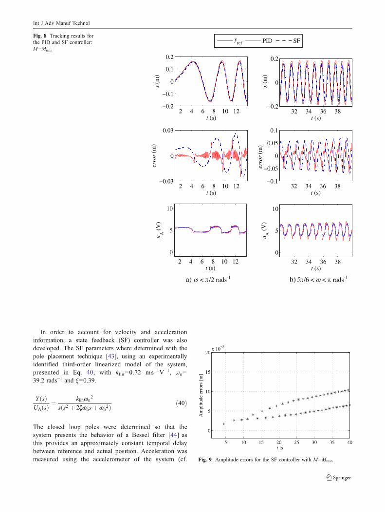
In order to establish the performance of the controllerdeveloped in this work, several trajectory following taskswere tested with three different loads:M=Mmin=2.69kg, M=Mmed=5.9kg, and M=Mmax=13.1 kg. The position referenceis a sinusoid with amplitude of 0.16 m and a progressivelyincreasing frequency at a rate of 0.0286×π rads−1/s (up to ca.π rad/s). For the sake of comparison, the trajectoriesfollowing tasks were tested not only with the controllerdeveloped in this work but also with two referencecontrollers: a PID and a state feedback controller, presentedin the next section.

4.1 Datum controllers

Both reference controllers where tuned for the minimummass configuration as this leads to the system maximumbandwidth. Furthermore, symmetrical control actions wereapplied to the servovalves, i.e., uA=−uB. The PID wastuned in two steps: first the Ziegler Nichols rules [43]where applied and then a fine experimental adjustment wasperformed. The final controller parameters are presented inTable 2.

Table 2 PID and SF controller parameters

PID kp=25.2 Vm−1 Td=0.02 s Ti=0.08 s

SF k1=462.7 Vm−1 k2=12.9 Vm−1 s k3=0.15 Vm−1 s2

Int J Adv Manuf Technol

In order to account for velocity and accelerationinformation, a state feedback (SF) controller was alsodeveloped. The SF parameters where determined with thepole placement technique [43], using an experimentallyidentified third-order linearized model of the system,presented in Eq. 40, with klin=0.72 ms−1V−1, ωn=39.2 rads−1 and ξ=0.39.

Y ðsÞUAðsÞ ¼

klinwn2

sðs2 þ 2xwnsþ wn2Þ ð40Þ

The closed loop poles were determined so that thesystem presents the behavior of a Bessel filter [44] asthis provides an approximately constant temporal delaybetween reference and actual position. Acceleration wasmeasured using the accelerometer of the system (cf.

2 4 6 8 10 12−0.2

−0.1

0

0.1

0.2

t (s)

x (m

)

2 4 6 8 10 12−0.03

0

0.03

t (s)

erro

r (m

)

2 4 6 8 10 12

0

5

10

t (s)

u A (

V)

32 34 36 38−0.2

0

0.2

t (s)

x (m

)

32 34 36 38−0.1

−0.05

0

0.05

0.1

t (s)

erro

r (m

)32 34 36 38

0

5

10

t (s)u A

(V

)

yref PID SF

a) < /2 rads-1 b) 5 /6 < < rads-1

Fig. 8 Tracking results forthe PID and SF controller:M=Mmin

5 10 15 20 25 30 35 40

0

5

10

15

20x 10

−3

t [s]

Am

plitu

de e

rror

s [m

]

Fig. 9 Amplitude errors for the SF controller with M=Mmin

Int J Adv Manuf Technol

Section 2.1) and velocity was measured using a stateobserver as presented in [45]. Table 2 resumes the SFparameters.

Figures 8 and 9 present results of the PID and SFcontrollers for Mmin, Fig. 10 for Mmed, and Fig. 11 Mmax.Notice that with the PID and M=Mmax, the piston collidedseveral times with the cylinder heads so the trial wasstopped after only ca. 10 s. Regarding the PID results, it ispossible to see that for M=Mmin the maximum followingerror is ca. 15 mm for low frequencies and ca. 50 mm forhigher frequencies. The maximum error occurs mainlywhen velocity changes sign, emphasizing the important rolethat static friction plays in the system. The PID performancewhen M=Mmed and M=Mmax is significantly deteriorated, afact that is expected since the PID does not accommodate

significant parameter variation. These trials highlight theneed of a PID retuning for each different mass used.Concerning the SF controller, overall results are clearlybetter than the ones obtained with the PID, revealing theimportance of velocity and acceleration feedback. In order toremove the influence of the time delays between referenceand measured positions from the analysis, Fig. 9 presents theerrors between the amplitude values of xref and the amplitudevalues of x for the trial of Fig. 8. It can be seen that the errorranges from ca. 2 mm to ca. 10 mm and steadily increaseswith frequency. Another noticeable feature is that the SFcontroller results appear to be highly independent of the loadfor the frequency range considered. This fact may once againbe justified by the existence velocity and accelerationfeedback.

2 4 6 8 10 12−0.2

−0.1

0

0.1

0.2

t (s)

x (m

)

2 4 6 8 10 12−0.03

0

0.03

t (s)

erro

r (m

)

2 4 6 8 10 12

0

5

10

t (s)

u A (

V)

32 34 36 38−0.2

−0.1

0

0.1

0.2

t (s)

x (m

)

32 34 36 38−0.1

−0.05

0

0.05

0.1

t (s)

erro

r (m

)32 34 36 38

0

5

10

t (s)u A

(V

)

yref PID SF

a) < /2 rads-1 b) 5 /6 < < rads-1

Fig. 10 Tracking results for thePID and SF controller: M=Mmed

Int J Adv Manuf Technol

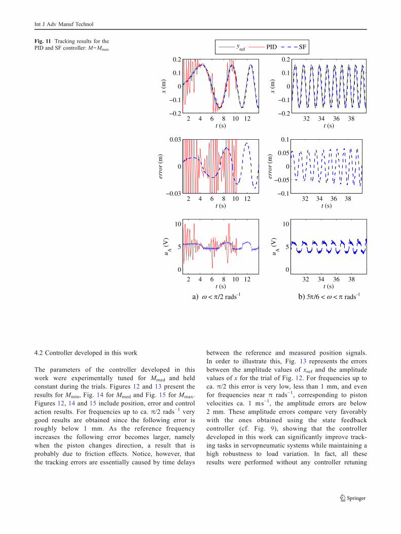
4.2 Controller developed in this work

The parameters of the controller developed in thiswork were experimentally tuned for Mmed and heldconstant during the trials. Figures 12 and 13 present theresults for Mmin, Fig. 14 for Mmed and Fig. 15 for Mmax.Figures 12, 14 and 15 include position, error and controlaction results. For frequencies up to ca. π/2 rads−1 verygood results are obtained since the following error isroughly below 1 mm. As the reference frequencyincreases the following error becomes larger, namelywhen the piston changes direction, a result that isprobably due to friction effects. Notice, however, thatthe tracking errors are essentially caused by time delays

between the reference and measured position signals.In order to illustrate this, Fig. 13 represents the errorsbetween the amplitude values of xref and the amplitudevalues of x for the trial of Fig. 12. For frequencies up toca. π/2 this error is very low, less than 1 mm, and evenfor frequencies near π rads−1, corresponding to pistonvelocities ca. 1 ms−1, the amplitude errors are below2 mm. These amplitude errors compare very favorablywith the ones obtained using the state feedbackcontroller (cf. Fig. 9), showing that the controllerdeveloped in this work can significantly improve track-ing tasks in servopneumatic systems while maintaining ahigh robustness to load variation. In fact, all theseresults were performed without any controller retuning

2 4 6 8 10 12−0.2

−0.1

0

0.1

0.2

t (s)

x (m

)

2 4 6 8 10 12−0.03

0

0.03

t (s)

erro

r (m

)

2 4 6 8 10 12

0

5

10

t (s)

u A (

V)

32 34 36 38−0.2

−0.1

0

0.1

0.2

t (s)

x (m

)

32 34 36 38−0.1

−0.05

0

0.05

0.1

t (s)

erro

r (m

)

32 34 36 38

0

5

10

t (s)

u A (

V)

yref PID SF

a) < /2 rads-1 b) 5 /6 < < rads-1

Fig. 11 Tracking results for thePID and SF controller: M=Mmax

Int J Adv Manuf Technol

although the load varies almost 500%. Regardingcontrollers developed in other research studies, a directcomparison is not possible as the reference type,amplitude, and frequency may differ substantially fromthe ones used in this work. However, and as detailedin Section 1, most studies present following errors in therange between 2 and 10 mm, so it is believed that theresults obtained in this work may represent a significantstep towards a more ample use of servopneumaticsystems in trajectory following industrial applications.A final remark to underline that the results presented inthis section are representative of the system performancesince similar conclusions were obtained with referencesof different amplitudes and shapes.

2 4 6 8 10 12

−0.1

0

0.1

t (s)

x (m

)

2 4 6 8 10 12−0.002

−0.001

0

0.001

0.002

t (s)

erro

r (m

)

2 4 6 8 10 12

0

5

10

t (s)

u (V

)

32 34 36 38

−0.1

0

0.1

t (s)

x (m

)

32 34 36 38−0.01

−0.005

0

0.005

0.01

t (s)

erro

r (m

)32 34 36 38

0

5

10

t (s)u

(V)

yref y

uA

uB

a) < /2 rads-1 b) 5 /6 < < rads-1

Fig. 12 Tracking results for thecontroller developed in thiswork: M=Mmin

5 10 15 20 25 30 35 40−2

−1.5

−1

−0.5

0

0.5

1

1.5

2x 10

−3

t [s]

Am

plitu

de e

rror

s [m

]

Fig. 13 Amplitude errors for M=Mmin

Int J Adv Manuf Technol

5 Conclusions

This paper presented an innovative controller for a pneumaticservosystem that achieves high performance in trajectoryfollowing tasks. After presenting the neural network-basedsystem model, an original control architecture with threecomponents (motion controller, force division block, andforce controller) was developed. The controller performancewas subsequently assessed in an experimental setup usingstandard industrial servopneumatic components. For compar-ison purposes two datum controllers (PID and state feedback)

were also developed and experimentally tested. Resultsshowed that a sinusoidal position reference with varyingfrequency can be followed, for frequencies up to π rads−1

(corresponding to piston velocities of ca. 1 ms−1), with errorsof only a few millimeters. This performance is much betterthan the one obtained with the datum controllers andcompares very favorably with existing literature results.Furthermore, the controlled system exhibited high robustnessto parameter variation since high accuracy results wereobtained without any controller retuning even though thepayload varied from 2.6 to 13.1 kg.

2 4 6 8 10 12

−0.1

0

0.1

t (s)

x (m

)

2 4 6 8 10 12

−1

0

1

x 10−3

t (s)

erro

r (m

)

2 4 6 8 10 12

0

5

10

t (s)

u (V

)

32 34 36 38

−0.1

0

0.1

t (s)

x (m

)

32 34 36 38

−5

0

5

x 10−3

t (s)

erro

r (m

)

32 34 36 38

0

5

10

t (s)

u (V

)

yref y

uA

uB

a) < /2 rads-1 b) 5 /6 < < rads-1

Fig. 14 Tracking results for thecontroller developed in thiswork: M=Mmed

Int J Adv Manuf Technol

References

1. Kagawa T, Tokashiki L, Fujita T (2000) Accurate positioning of apneumatic servosystem with air bearings. In: Proc. of the BathWorkshop on Power Transmission and Motion Control, Bath, UK,2000. pp 257–268

2. Sorli M, Figliolini G, Almondo A (2010) Mechatronic model andexperimental validation of a pneumatic servo-solenoid valve.ASME J Dyn Syst, Meas, Control 132(5):054503

3. Richard E, Scavarda S (1996) Comparison between linear andnonlinear control of an electropneumatic servodrive. ASME J DynSyst, Meas, Control 118(2):245–252

4. Thomasset D, Scavarda S, Sesmat S, Belgharbi M (1999)Analytical model of the flow stage of a pneumatic servo-distributor for simulation and nonlinear control. In: Proc. of theSixth Scandinavian International Conference on Fluid PowerTampere, Finland, May 26–28 1999. pp 848–860

5. Carneiro JF, Almeida FG (2006) Modeling Pneumatic Servo-valves using Neural Networks. In: Proc. of the 2006 IEEEConference on Computer Aided Control Systems Design, Munich,Germany, 2006. pp 790–795

6. Carneiro JF, Almeida FG (2006) Pneumatic servovalve modelsusing artificial neural networks. In: Johnston N, Edge K (eds)Proc. of the Bath Symposium on Power Transmission and MotionControl. Bath, UK, pp 195–208

7. Karnopp D (1985) Computer simulation of stick-slip friction inmechanical dynamic systems. ASME J Dyn Syst, Meas, Control107(1):100–107

8. Canudas de Wit C, Olsson H, Astrom K, Lischinsky P (1995) Anew model for control of systems with friction. IEEE Transactionson Automatic Control 40(3):419–425

9. Swevers J, Al-Bender F, Ganseman CG, Prajogo T (2000) Anintegrated friction model structure with improved preslidingbehavior for accurate friction compensation. IEEE Transactionson Automatic Control 45(4):675–686

2 4 6 8 10 12

−0.1

0

0.1

t (s)

x (m

)

yref y

2 4 6 8 10 12

−1

0

1

x 10−3

t (s)

erro

r (m

)

2 4 6 8 10 12

0

5

10

t (s)

u (V

)

32 34 36 38

−0.1

0

0.1

t (s)

x (m

)

32 34 36 38−5

0

5x 10

−3

t (s)

erro

r (m

)

32 34 36 38

0

5

10

t (s)

u (V

)

uA

uB

b) 5 /6 < < rads-1a) < /2 rads-1

Fig. 15 Tracking results for thecontroller developed in thiswork: M=Mmax

Int J Adv Manuf Technol

10. Richer E, Hurmuzlu Y (2000) A high performance pneumaticforce actuator system: part I—nonlinear mathematical model.ASME J Dyn Syst, Meas, Control 122(3):416–425

11. Carneiro JF, Almeida FG (2006) Reduced order thermodynamicmodels for servopneumatic actuator chambers. Proc Instn MechEngrs, Part I, Journal of Systems and Control Engineering 220(4):301–314

12. Najafi F, Morteza F, Saadat M (2009) Dynamic modelling ofservo pneumatic actuators with cushioning. International Journalof Advance Manufacturing Technology 42(7–8):757–765

13. Saleem A, Abdrabbo S, Tutunji T (2009) On-line identificationand control of pneumatic servo drives via a mixed-realityenvironment. International Journal of Advanced ManufacturingTechnology 40(5–6):518–530

14. Takosoglu J, Dindorf R, Laski P (2010) Rapid prototyping offuzzy controller pneumatic servo-system. International Journal ofAdvanced Manufacturing Systems 40(3–4):349–361

15. Pu J, Weston RH (1988) Motion control of pneumatic drives.Microprocessors and Microsystems 12(7):373–382

16. Ionnidis I, Nguyen T (1986) Microcomputer-controlled servo-pneumatic drives. In: Seventh International Fluid Power Sympo-sium, September 1986. pp 155–164

17. Ning S, Bone G (2002) High Steady-State Accuracy PneumaticServo Positioning System with PVA/PV Control and FrictionCompensation. In: Proc. of the 2002 IEEE International Confer-ence on Robotics and Automation, Washington DC, USA, 2002.pp 2824–2829

18. Isidori A (1995) Nonlinear control systems 3rd edn. Springer,New York

19. Slotine JJ, Li W (1991) Applied nonlinear control. Prentice-Hall,New Jersey

20. Outbib R, Richard E (2000) State feedback stabilization of anelectropneumatic system. ASME J Dyn Syst, Meas, Control 122(3):410–415

21. Xiang F, Wikander J (2004) Block-oriented approximate feedbacklinearization for control of pneumatic actuator system. ControlEngineering Practice 12(4):387–399

22. Situm Z, Pavkovic D, Novakovic B (2004) Servo pneumaticposition control using fuzzy PID gain scheduling. ASME J DynSyst, Meas, Control 126(2):376–387

23. Taghizadeh M, Najafi F, Ghaffari A (2010) Multimodel PD-control of a pneumatic actuator under variable loads. Intern-tional Journal of Advanced Manufacturing Technologies48:655–662

24. Bobrow JE, Jabbari F (1991) Adaptive pneumatic force actuationand position control. ASME J Dyn Syst, Meas, Control 113(2):267–272

25. Shih M-C, Shy-I T (1994) Pneumatic servo-cylinder positioncontrol by PID-self-tuning controller. Japan Society of MechanicalEngineers International Journal 37(3):565–572

26. Ferraresi C, Giruado P, Quaglia G (1994) Non-conventionaladaptive control of a servopneumatic unit for vertical loadpositioning. In: Proc. of the 46th National Conference on FluidPower, 1994. pp 319–333

27. Richardson R, Plummer A, Brown M (2001) Self-tuning controlof a low-friction pneumatic actuator under the influence ofgravity. IEEE Transactions on Control Systems Technology 9(2):330–334

28. Drakunov S, Hanchin GD, Su WC, Ozguner U (1997) Nonlinearcontrol of a rodless pneumatic servoactuator, or sliding modesversus Coulomb friction. Automatica 33(7):1401–1408

29. Pandian S, Hayakawa Y, Kanazawa Y, Kamoyama Y, KawamuraS (1997) Practical design of a sliding mode controller forpneumatic actuators. ASME J Dyn Syst, Meas, Control 119(4):666–674

30. Richer E, Hurmuzlu Y (2000) A high performance pneumaticforce actuator system: part II—nonlinear controller design. ASMEJ Dyn Syst, Meas, Control 122(3):426–434

31. Levant A (1993) Sliding order and sliding accuracy in slidingmode control. International Journal of Control 58(6):1247–1263

32. Smaoui M, Brun X, Thomasset D (2004) Robust Position Controlof an Electropneumatic System Using Second Order SlidingMode. In: Proc. of the 2004 IEEE International Symposium onIndustrial Electronics, Ajaccio, France, 2004. pp 429–434

33. Junbo S, Xiaoyan B, Ishida Y (1997) An application of MNNtrained by MEKA for the position control of pneumatic cylinder.In: Proc. of the IEEE International Conference on NeuralNetworks, Houston, USA, 1997. pp 829–833

34. Lee HK, Choi GS, Choi GH (2002) A study on tracking positioncontrol of pneumatic actuators. Mechatronics 12(6):813–831

35. Varseveld R, Bone GM (1997) Accurate position control of apneumatic actuator using on/off solenoid valves. IEEE/ASMETransactions on Mechatronics 2(3):195–204

36. Reina G, Giannoccaro NI, Gentile A (2002) Experimental tests onposition control of a pneumatic actuator using on/off solenoidvalves. In: Proc. of the IEEE International Conference onIndustrial Technology, Bangkok, Thailand, 2002. pp 555–559

37. Carneiro JF, Gomes de Almeida F (2011) Pneumatic servo valvemodels based on artificial neural networks. Proceedings of theInstitution of Mechanical Engineers, Part I: Journal of Systemsand Control Engineering 225(3):393–411. doi:10.1177/2041304110394498

38. Noorgard M, Ravn O, Poulsen NK, Hansen LK (2003) Neuralnetworks for modelling and control of dynamic systems: apractitioner’s handbook. Springer Verlag, London

39. Carneiro JF, Almeida FG (2007) Heat transfer evaluation onindustrial pneumatic cylinders. Proc Instn Mech Engrs, Part I,Journal of Systems and Control Engineering 221(1):119–128

40. Brun X, Thomasset D, Bideaux E (2002) Influence of the processdesign on the control strategy: application in electropneumaticfield. Control Engineering Practice 10(7):727–735

41. Barth EJ, Goldfarb M, Al-Dakkan KA (2003) Energy SavingControl for Pneumatic Servo Systems. In: Proc. of the 2003 IEEE/ASME International Conference on Advanced Mechatronics,Kobe, Japan, 2003. pp 284–289

42. Carneiro JF, Almeida FG (2011) Vsc approach angle based boundarylayer thickness: a new variation law and its stability proof. In:Accepted for publication on the 2011 Bath/ASME Symposium onFluid Power and Motion Control, Arlington, VA, 2011.

43. Ogata K (2001) Modern control engineering 4th edn. PrenticeHall,

44. Schaumann R, Valkenburg MEV (2001) Design of analog filters.Oxford University Press, Inc., New York

45. Lopes AM, Almeida FG (2007) Acceleration-based force-impedance control of a six-dof parallel manipulator. IndustrialRobot: An International Journal 34(5):386–399

Int J Adv Manuf Technol