A High-Purity Germanium Imaging System By Desmond...

A High-Purity Germanium Imaging Systemfor Limited-Angle Nuclear Breast Tomography

By

Desmond L. Campbell

Dissertation

Submitted to the Faculty of the

Graduate School of Vanderbilt University

in partial fulfillment of the requirements

for the degree of

DOCTOR OF PHILOSOPHY

in

Physics

May, 2015

Nashville, Tennessee

Approved:

Professor Todd Peterson

Professor Arnold Burger

Professor David Ernst

Professor Julia Velkovska

Professor Thomas Yankeelov

To my loving family,

to my friends near and far

and

to my supportive wife

ii

ACKNOWLEDGMENTS

The work discussed in this dissertation has been supported by the following en-

tities and funding sources: NIH/NIBIB R44EB15889, NIH/NCI R25CA136440, the

Graduate Assistance in Areas of National Need fellowship, the Department of Physics

and Astronomy, and the Southern Region Education Board. The work was conducted

in part using the resources of the Advanced Computing Center for Research and Ed-

ucation at Vanderbilt University, Nashville, TN.

I have thoroughly enjoyed my time at Vanderbilt. The past six years learning and

working with Dr. Todd Peterson has afforded me some of the best experiences of my

life. I am eternally grateful for his guidance and assistance with this work. I would

also like to extend my thanks to the members of my dissertation committee, Dr.

Arnold Burger, Dr. David Ernst, Dr. Julia Velkovska, and Dr. Thomas Yankeelov,

for their insightful comments and suggestions during my graduate tenure. I would

also like to thank all current and former members of the Ionizing Imaging group,

Dr. Lindsay Johnson, Dr. Sepideh Shokouhi, Dr. M. Noor Tantawy, Dr. Benjamin

McDonald, Oleg Ochinnikov, and Rose Perea. Additionally, I would like to recognize

the Vanderbilt University Institute of Imaging Science for their graduate education

and training programs, which have enriched my understanding of physics and the

biomedical sciences. I also greatly appreciate the efforts made by Ethan Hull at

PHDs Co. and Ben Welch at Dilon Technologies and thank them for their support

and assistance through this work.

iii

The support offered by the faculty, post-docs, coordinators, and members of the

Fisk-Vanderbilt Bridge program have sustained me through this journey. The people

of the ”Bridge Family” are incredible and it has been an honor to learn and grow

with all of you. To my friends near and far, thank you as well. Your encouragement

and kind words have provided me with strength to endure all challenges. And finally

to my family, thank you for your continuous and unyielding faith in me. I hope I

have made you proud.

iv

TABLE OF CONTENTS

Page

DEDICATION . . . . . . . . . . . . . . . . . . . . . . . . . . . . . . . . . . . iii

ACKNOWLEDGMENTS . . . . . . . . . . . . . . . . . . . . . . . . . . . . . v

LIST OF TABLES . . . . . . . . . . . . . . . . . . . . . . . . . . . . . . . . . viii

LIST OF FIGURES . . . . . . . . . . . . . . . . . . . . . . . . . . . . . . . . ix

Chapter

I. Introduction and Background . . . . . . . . . . . . . . . . . . . . . . . 1

1.1. Radionuclide Imaging Overview . . . . . . . . . . . . . . . . . . . . 51.1.1. Relevant Imaging Properties . . . . . . . . . . . . . . . . . . . . 7

1.2. Radiation Detectors . . . . . . . . . . . . . . . . . . . . . . . . . . . 91.2.1. Scintillators . . . . . . . . . . . . . . . . . . . . . . . . . . . . . 91.2.2. Semiconductors . . . . . . . . . . . . . . . . . . . . . . . . . . . 12

1.3. Germanium Gamma Camera History . . . . . . . . . . . . . . . . . 181.4. Breast Cancer Imaging . . . . . . . . . . . . . . . . . . . . . . . . . 23

1.4.1. X-Ray Mammography . . . . . . . . . . . . . . . . . . . . . . . 231.4.2. Alternative Imaging Modalities . . . . . . . . . . . . . . . . . . 261.4.3. Nuclear Breast Imaging Methods . . . . . . . . . . . . . . . . . 291.4.4. Limited-Angle Nuclear Breast Tomography . . . . . . . . . . . . 41

II. General Radiation Transport and Analysis Methods . . . . . . . . . . . 48

2.1. Monte-Carlo N-Particle Simulator . . . . . . . . . . . . . . . . . . . 482.1.1. MCNP5 Overview . . . . . . . . . . . . . . . . . . . . . . . . . . 482.1.2. MCNP5 Inputs . . . . . . . . . . . . . . . . . . . . . . . . . . . 492.1.3. Particle Track Output Card . . . . . . . . . . . . . . . . . . . . 60

2.2. MATLAB PTRAC Parser . . . . . . . . . . . . . . . . . . . . . . . 632.3. Imaging Metrics and Analysis . . . . . . . . . . . . . . . . . . . . . 64

2.3.1. Pulse Height Spectrum . . . . . . . . . . . . . . . . . . . . . . . 642.3.2. Image Formation . . . . . . . . . . . . . . . . . . . . . . . . . . 65

2.4. Chapter Summary . . . . . . . . . . . . . . . . . . . . . . . . . . . . 67

v

III. Germanium Detector Characterization . . . . . . . . . . . . . . . . . . 68

3.1. Introduction . . . . . . . . . . . . . . . . . . . . . . . . . . . . . . . 683.2. Materials and Methods . . . . . . . . . . . . . . . . . . . . . . . . . 70

3.2.1. System Specifications . . . . . . . . . . . . . . . . . . . . . . . . 703.2.2. Intrinsic Detector Measurements . . . . . . . . . . . . . . . . . . 723.2.3. Camera Measurements . . . . . . . . . . . . . . . . . . . . . . . 75

3.3. Experimental Results . . . . . . . . . . . . . . . . . . . . . . . . . . 793.3.1. Intrinsic Detector Measurements . . . . . . . . . . . . . . . . . . 793.3.2. Camera Measurements . . . . . . . . . . . . . . . . . . . . . . . 84

3.4. Discussion . . . . . . . . . . . . . . . . . . . . . . . . . . . . . . . . 893.5. Chapter Summary . . . . . . . . . . . . . . . . . . . . . . . . . . . . 91

IV. Investigating Potential Benefits of Germanium Cameras for Breast Imaging 93

4.1. Introduction . . . . . . . . . . . . . . . . . . . . . . . . . . . . . . . 934.2. Monte Carlo Model Development . . . . . . . . . . . . . . . . . . . 95

4.2.1. HPGe Camera Model . . . . . . . . . . . . . . . . . . . . . . . . 964.2.2. Experimental Validation . . . . . . . . . . . . . . . . . . . . . . 97

4.3. Nuclear Breast Imaging Simulations . . . . . . . . . . . . . . . . . . 1004.3.1. Breast Phantom Parameters . . . . . . . . . . . . . . . . . . . . 1004.3.2. CZT Camera Model . . . . . . . . . . . . . . . . . . . . . . . . 1024.3.3. Simulation Measurements and Analysis . . . . . . . . . . . . . . 103

4.4. Experimental and Simulation Results . . . . . . . . . . . . . . . . . 1044.4.1. Experimental Validation . . . . . . . . . . . . . . . . . . . . . . 1044.4.2. Generated Energy Spectral Analysis . . . . . . . . . . . . . . . . 1074.4.3. Simulated Images . . . . . . . . . . . . . . . . . . . . . . . . . . 1104.4.4. Image Performance . . . . . . . . . . . . . . . . . . . . . . . . . 1124.4.5. Equal Sensitivity Imaging Performance . . . . . . . . . . . . . . 112


V. Parallel-Hole Collimator Design and Selection for Germanium Detectors 123

5.1. Introduction . . . . . . . . . . . . . . . . . . . . . . . . . . . . . . . 1235.2. Materials and Methods . . . . . . . . . . . . . . . . . . . . . . . . . 125

5.2.1. Collimator Designs . . . . . . . . . . . . . . . . . . . . . . . . . 1255.2.2. Simulation Details . . . . . . . . . . . . . . . . . . . . . . . . . 131

5.3. Simulation Results . . . . . . . . . . . . . . . . . . . . . . . . . . . 1355.3.1. NBI Energy Spectra . . . . . . . . . . . . . . . . . . . . . . . . 1355.3.2. NBI Projections . . . . . . . . . . . . . . . . . . . . . . . . . . . 1375.3.3. Contrast-Detail Simulations . . . . . . . . . . . . . . . . . . . . 141

5.4. Discussion . . . . . . . . . . . . . . . . . . . . . . . . . . . . . . . . 144

vi

5.5. Chapter Summary . . . . . . . . . . . . . . . . . . . . . . . . . . . . 149

VI. Limited-Angle Tomographic Breast Imaging with a HPGe Camera . . . 151

6.1. Introduction . . . . . . . . . . . . . . . . . . . . . . . . . . . . . . . 1516.2. Methods . . . . . . . . . . . . . . . . . . . . . . . . . . . . . . . . . 152

6.2.1. Limited-Angle Tomography . . . . . . . . . . . . . . . . . . . . 1526.2.2. System Matrix Generation . . . . . . . . . . . . . . . . . . . . . 1556.2.3. Simulation Details . . . . . . . . . . . . . . . . . . . . . . . . . 156

6.3. Results . . . . . . . . . . . . . . . . . . . . . . . . . . . . . . . . . . 1586.3.1. NBI Simulations . . . . . . . . . . . . . . . . . . . . . . . . . . 1586.3.2. Contrast-Detail Simulations . . . . . . . . . . . . . . . . . . . . 161


VII. A Dual-Head Germanium Imaging System . . . . . . . . . . . . . . . . 171

7.1. Introduction . . . . . . . . . . . . . . . . . . . . . . . . . . . . . . . 1717.2. Methods . . . . . . . . . . . . . . . . . . . . . . . . . . . . . . . . . 174

7.2.1. OSEM Reconstruction . . . . . . . . . . . . . . . . . . . . . . . 1757.2.2. Phantom Details . . . . . . . . . . . . . . . . . . . . . . . . . . 1767.2.3. Simulation Measurements and Analysis . . . . . . . . . . . . . . 178

7.3. Results . . . . . . . . . . . . . . . . . . . . . . . . . . . . . . . . . . 1797.3.1. NBI Simulations . . . . . . . . . . . . . . . . . . . . . . . . . . 1797.3.2. Contrast-Detail Simulations . . . . . . . . . . . . . . . . . . . . 192


VIII. Reflections and Conclusions . . . . . . . . . . . . . . . . . . . . . . . . 207

8.1. Dissertation Summary . . . . . . . . . . . . . . . . . . . . . . . . . 2078.2. Future Considerations and Endeavors . . . . . . . . . . . . . . . . . 212

REFERENCES . . . . . . . . . . . . . . . . . . . . . . . . . . . . . . . . . . . 215

vii

LIST OF TABLES

Table Page

1. Properties of select scintillators . . . . . . . . . . . . . . . . . . . . . . 12

2. Properties of select semiconductors . . . . . . . . . . . . . . . . . . . . 15

3. MCNP5 Surface Cards . . . . . . . . . . . . . . . . . . . . . . . . . . 50

4. MCNP5 Source Variables for the SDEF card . . . . . . . . . . . . . . 58

5. MI4 Flood Field Uniformity Measurements . . . . . . . . . . . . . . . 81

6. GGC Flood Field Uniformity Measurements . . . . . . . . . . . . . . 81

7. MI4 Spatial Response at 6.0 cm from the Parallel-Hole Collimator . . 86

8. GGC Spatial Response at 6.7 cm from the Parallel-Hole Collimator . . 86

9. Contrast and SNR values for hot spheres in images of the breast phantom 87

10. Source definitions for the breast/torso phantom. . . . . . . . . . . . . 102

11. Performance measures by detector type and energy window. . . . . . . 109

12. Collimator Dimensions and Theoretical Properties. . . . . . . . . . . . 130

13. Collimator performance measures for the ±2.5% energy window. . . . 136

14. Collimator performance measures for the ±1.25% energy window. . . . 136

15. Source definitions for the breast phantom with the dual-head HPGemodel. . . . . . . . . . . . . . . . . . . . . . . . . . . . . . . . . . . . 177

16. Relative count sensitivity, scatter, and torso fraction measurements. . 179

viii

LIST OF FIGURES

Figure Page

1. A schematic diagram of a radionuclide scan after injection of a radio-tracter. . . . . . . . . . . . . . . . . . . . . . . . . . . . . . . . . . . . 6

2. An in-vivo image of a rat thyroid acquired with an orthogonal-stripHPGe camera developed by J.F. Detko. . . . . . . . . . . . . . . . . . 19

3. An example waveform characterizing a single event absorbed in a double-sided strip Germanium detector. . . . . . . . . . . . . . . . . . . . . . 21

4. Photograph of a woman undergoing a conventional scintimammographyscan using general-purpose cameras. . . . . . . . . . . . . . . . . . . . 30

5. Examples of mammography and scintimammography employed to scanthe same patient. . . . . . . . . . . . . . . . . . . . . . . . . . . . . . 31

6. A photograph of a woman undergoing a BSGI scan using the Dilon 6800dedicated breast imager. . . . . . . . . . . . . . . . . . . . . . . . . . 33

7. Comparable images of the same patient acquired using mammographyand BSGI. . . . . . . . . . . . . . . . . . . . . . . . . . . . . . . . . . 34

8. A photograph of the MBI dual-head system, the LumaGem 3200S, uti-lizing CZT detectors. . . . . . . . . . . . . . . . . . . . . . . . . . . . 36

9. Direct comparison of the same breast imaged using standard x-raymammography and MBI. . . . . . . . . . . . . . . . . . . . . . . . . . 39

10. Photograph of the hybrid SPECT/CT breast imaging system. . . . . . 43

11. A photograph of the Dual Modality Tomosynthesis system. . . . . . . 45

12. An schematic illustrating Boolean Operations in MCNP5 . . . . . . . 52

13. A simple MCNP geometry consisting of spheres. Circle numbers aresurfaces and square numbers correspond to cells. . . . . . . . . . . . . 53

14. A timeline illustrating the HPGe systems fabricated and developed byPHDs Co. . . . . . . . . . . . . . . . . . . . . . . . . . . . . . . . . . 69

15. Photographs of the MI4 system. . . . . . . . . . . . . . . . . . . . . . 71

ix

16. Images of the GGC system. . . . . . . . . . . . . . . . . . . . . . . . . 72

17. A photograph of the 6-cm thick breast phantom with 1 mL and 0.25mL spheres inside. . . . . . . . . . . . . . . . . . . . . . . . . . . . . . 77

18. Representative flood illuminated projections from the MI4 and GGCHPGe detectors. . . . . . . . . . . . . . . . . . . . . . . . . . . . . . . 78

19. The pulse-height spectrum of 57Co acquired with the MI4 imaging system. 80

20. The pulse-height spectrum of multiple radinuclides acquired with theGGC imaging system. . . . . . . . . . . . . . . . . . . . . . . . . . . . 81

21. The intrinsic spatial resolution of the MI4 detector measured using theESF method. . . . . . . . . . . . . . . . . . . . . . . . . . . . . . . . . 82

22. The intrinsic spatial resolution of the GGC detector measured usingthe ESF method. . . . . . . . . . . . . . . . . . . . . . . . . . . . . . . 83

23. Processed images of the UFOV from the MI4 and GGC for determiningflood field uniformity. . . . . . . . . . . . . . . . . . . . . . . . . . . . 84

24. Projection images of capillary tubes and line spread functions demon-strating the spatial response of the MI4 and GGC detectors. . . . . . 85

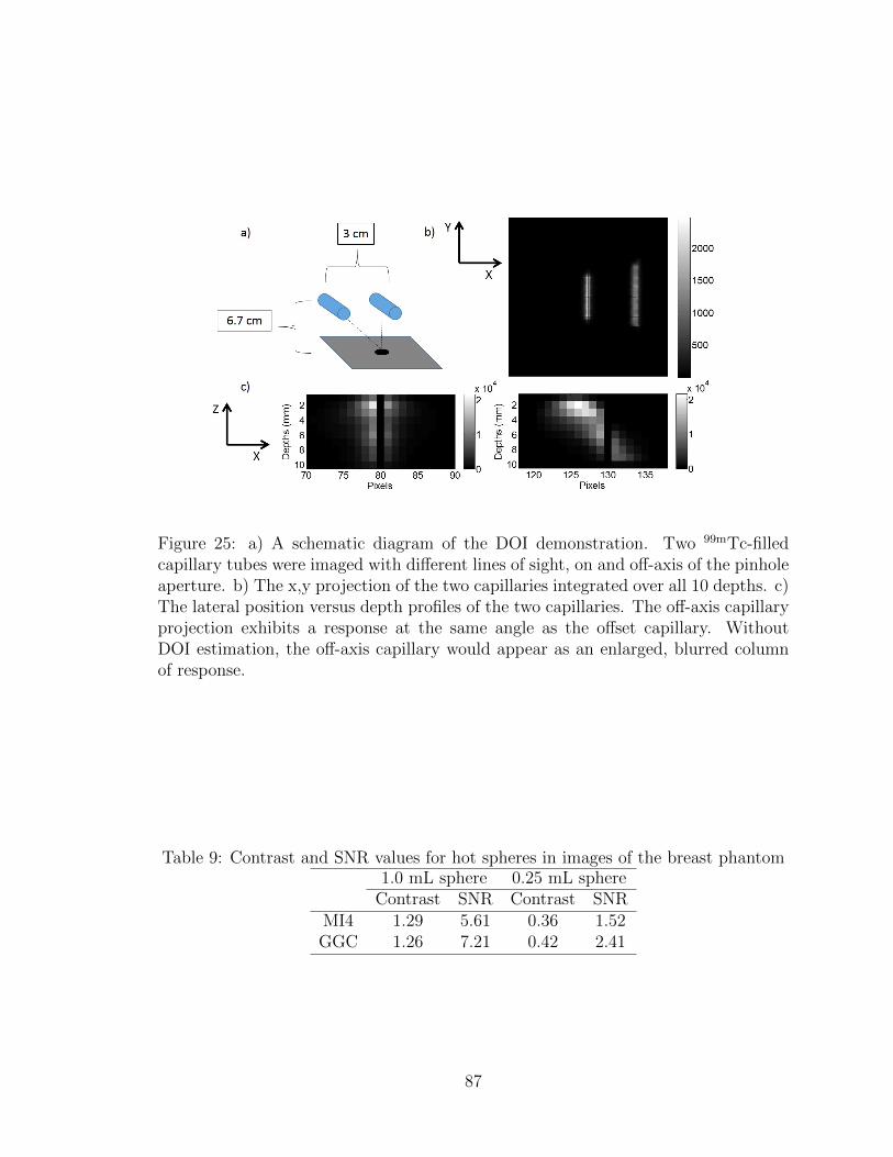
25. A schematic diagram and demonstration of the Depth-Of-Interactioncapabilities of the GGC. . . . . . . . . . . . . . . . . . . . . . . . . . . 87

26. Projection images of the breast phantom containing 0.25 mL and 1 mLhot spheres acquired with the MI4 and GGC. . . . . . . . . . . . . . . 88

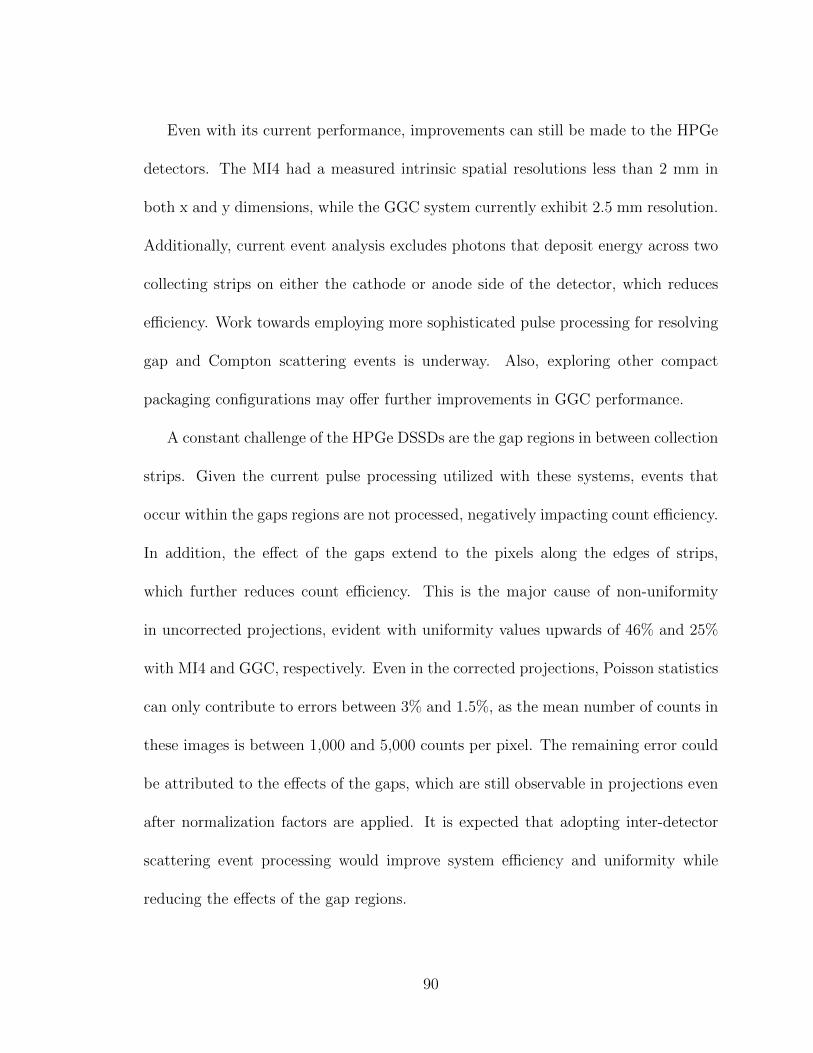
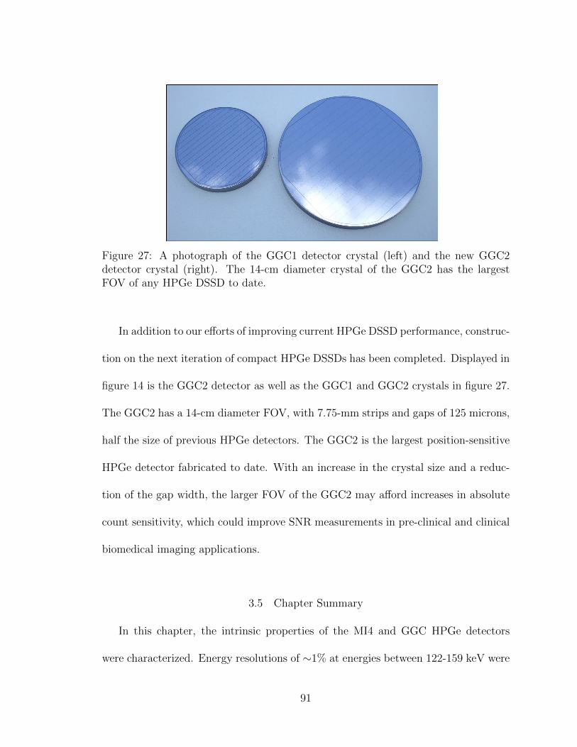
27. A photograph of the GGC1 detector crystal and the new GGC2 detectorcrystal. The GGC2 detector currently has the largest FOV of any HPGedetector to date. . . . . . . . . . . . . . . . . . . . . . . . . . . . . . . 91

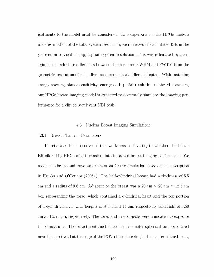
28. A schematic diagram of the geometry for the Monte Carlo breast imag-ing simulation comparing CZT and HPGe cameras. . . . . . . . . . . 101

29. Energy spectra acquired using a 99mTc source with the MI4 HPGe cam-era and the Monte Carlo simulation model. . . . . . . . . . . . . . . . 105

30. The total system resolution measurements along the x-axis and y-axis,and corrected system resolution for the y-axis. . . . . . . . . . . . . . 106

x

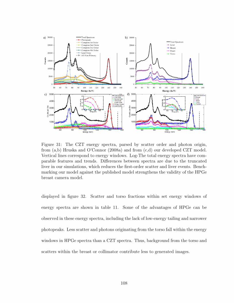
31. The CZT energy spectra from Hruska and O’Connor (2008a) and fromour CZT model. . . . . . . . . . . . . . . . . . . . . . . . . . . . . . . 108

32. Generated energy spectra from the breast imaging simulations. . . . . 109

33. Filtered breast images, with tumors at depths of either 1 cm or 4 cm,generated from one simulation run of the CZT and HPGe models. . . 110

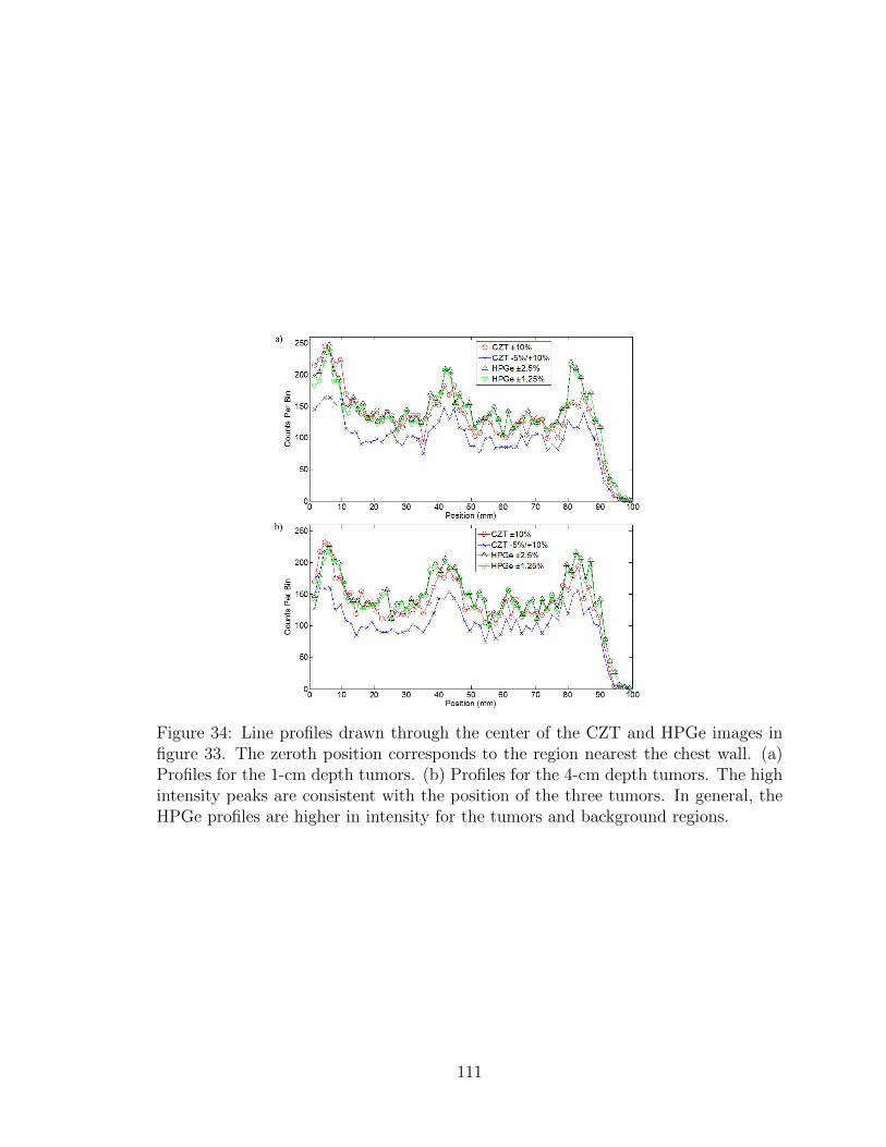
34. Line profiles drawn through the center of the CZT and HPGe imagesin figure 33. . . . . . . . . . . . . . . . . . . . . . . . . . . . . . . . . 111

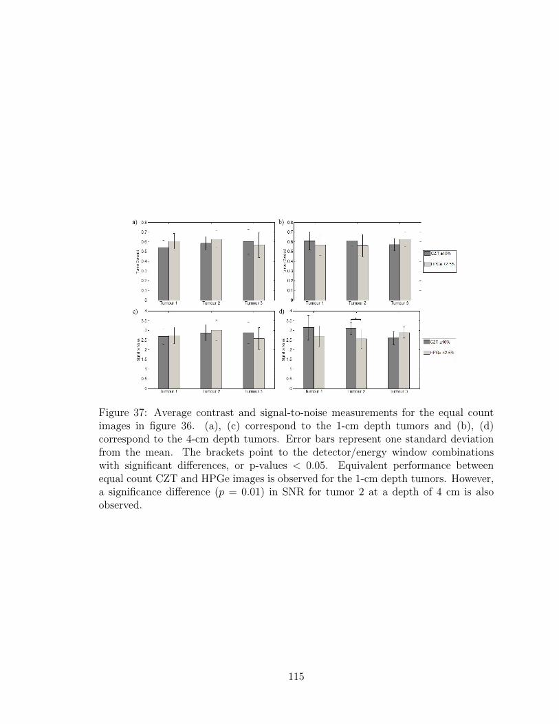
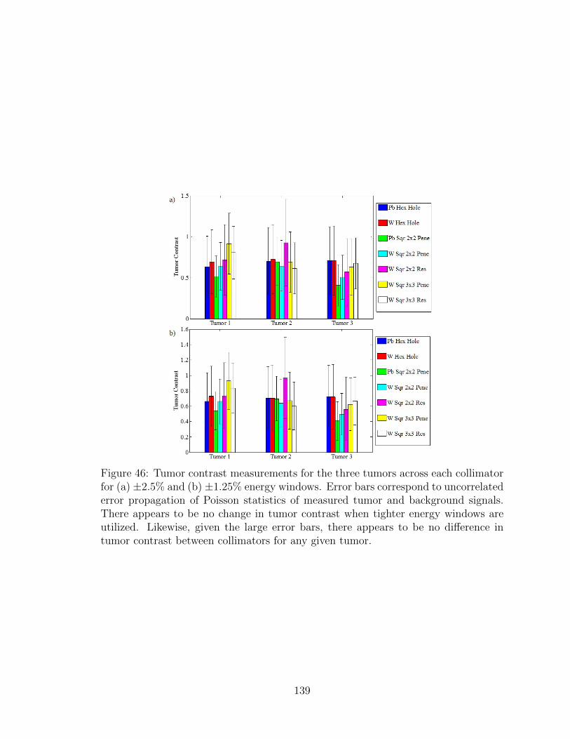
35. Average tumor contrast and signal-to-noise measurements for all com-binations of detector, tumor depth, and energy window across ten in-dependent simulations. . . . . . . . . . . . . . . . . . . . . . . . . . . 113

36. CZT- and HPGe-acquired breast phantom projections with equal countdensities. . . . . . . . . . . . . . . . . . . . . . . . . . . . . . . . . . . 114

37. Average contrast and signal-to-noise measurements for the equal countimages in figure 36. . . . . . . . . . . . . . . . . . . . . . . . . . . . . 115

38. A schematic diagram of the detector and parallel-hole collimator withlabeled parameters. . . . . . . . . . . . . . . . . . . . . . . . . . . . . 126

39. A visual representation of the collimator design process. . . . . . . . . 127

40. [A schematic diagram showing the minimal path length for photon pen-etration through a collimator septum. . . . . . . . . . . . . . . . . . . 128

41. Axial views of the standard lead hexagonal-hole collimator and twotungsten square-hole collimators. . . . . . . . . . . . . . . . . . . . . . 130

42. An axial view of the contrast-detail phantom. . . . . . . . . . . . . . . 132

43. Generated energy spectra parsed by scatter order of the breast/torsophantom acquired with the HPGe model mounted to select collimators. 133

44. Generated energy spectra parsed by event origin of the breast/torsophantom acquired with the HPGe model mounted to select collimators. 134

45. Generated projections of the breast/torso phantom acquired from theHPGe model with each collimator. . . . . . . . . . . . . . . . . . . . . 138

46. Tumor contrast measurements for the three tumors across each colli-mator for the (a) ±2.5% and (b) ±1.25% energy windows. . . . . . . . 139

xi

47. Tumor SNR measurements for the three tumors across each collimatorfor the (a) ±2.5% and (b) ±1.25% energy windows. . . . . . . . . . . 140

48. Generated projections of the contrast-detail phantom acquired with theHPGe model with each collimator. . . . . . . . . . . . . . . . . . . . . 141

49. Horizontal and vertical line profiles through the contrast-detail projec-tion images. (a) 10:1 TBR tumors, (b) 6-mm diameter tumors. . . . . 142

50. Tumor contrast measurements from the contrast-detail phantom pro-jections. (a) 3:1 TBR, (b) 5:1 TBR, (c) 10:1 TBR, (d) 15:1 TBR, (e)20:1 TBR. . . . . . . . . . . . . . . . . . . . . . . . . . . . . . . . . . 143

51. Tumor SNR measurements from the contrast-detail phantom projec-tions. (a) 3:1 TBR, (b) 5:1 TBR, (c) 10:1 TBR, (d) 15:1 TBR, (e) 20:1TBR. . . . . . . . . . . . . . . . . . . . . . . . . . . . . . . . . . . . . 144

52. A Schematic diagram showing the camera geometries with the tradi-tional planar and the limited-angle tomographic acquisition. . . . . . . 153

53. A schematic diagram of the inverse image problem with the voxelizedobject, voxelized detector, and collimator. . . . . . . . . . . . . . . . . 155

54. The NMSE curve with the contrast and SNR curves by iteration for thereconstructed breast image with perfect spatial resolution. . . . . . . . 158

55. The third iteration of the maximum-intensity projection and repro-jected breast image with perfect spatial resolution. . . . . . . . . . . . 159

56. Tumor contrast and SNR measurements for the NBI simulations withperfect spatial resolution. . . . . . . . . . . . . . . . . . . . . . . . . . 160

57. The NMSE curve with the contrast and SNR curves by iteration forreconstructed breast images with an lateral 1.5-mm spatial resolution. 160

58. The planar projection and the third iteration of the maximum-intensityprojection and reprojected breast image with perfect spatial resolution. 161

59. Tumor contrast and SNR measurements for the NBI simulations with1.5-mm spatial resolution. . . . . . . . . . . . . . . . . . . . . . . . . . 162

60. The NMSE curve for the contrast-detail image with perfect spatial res-olution and the axial and coronal slices of the 4th iteration. . . . . . . 162

xii

61. The fourth iteration of the maximum-intensity projection and repro-jected contrast-detail image with perfect spatial resolution. . . . . . . 163

62. Line profiles through the 6-mm and 10:1 TBR hot spots in the repro-jected and MIP contrast-detail images with perfect spatial resolution. 164

63. Tumor detectability based upon SNR and minimum TBR and diameterfor the reconstructed contrast-detail projections with perfect spatialresolution. . . . . . . . . . . . . . . . . . . . . . . . . . . . . . . . . . 164

64. The NMSE curve for the contrast-detail image with 1.5-mm spatialresolution and the axial and coronal slices of the 4th iteration. . . . . 165

65. The planar projection and the fourth iteration of the maximum-intensityprojection and reprojected contrast-detail image with 1.5-mm spatialresolution. . . . . . . . . . . . . . . . . . . . . . . . . . . . . . . . . . 165

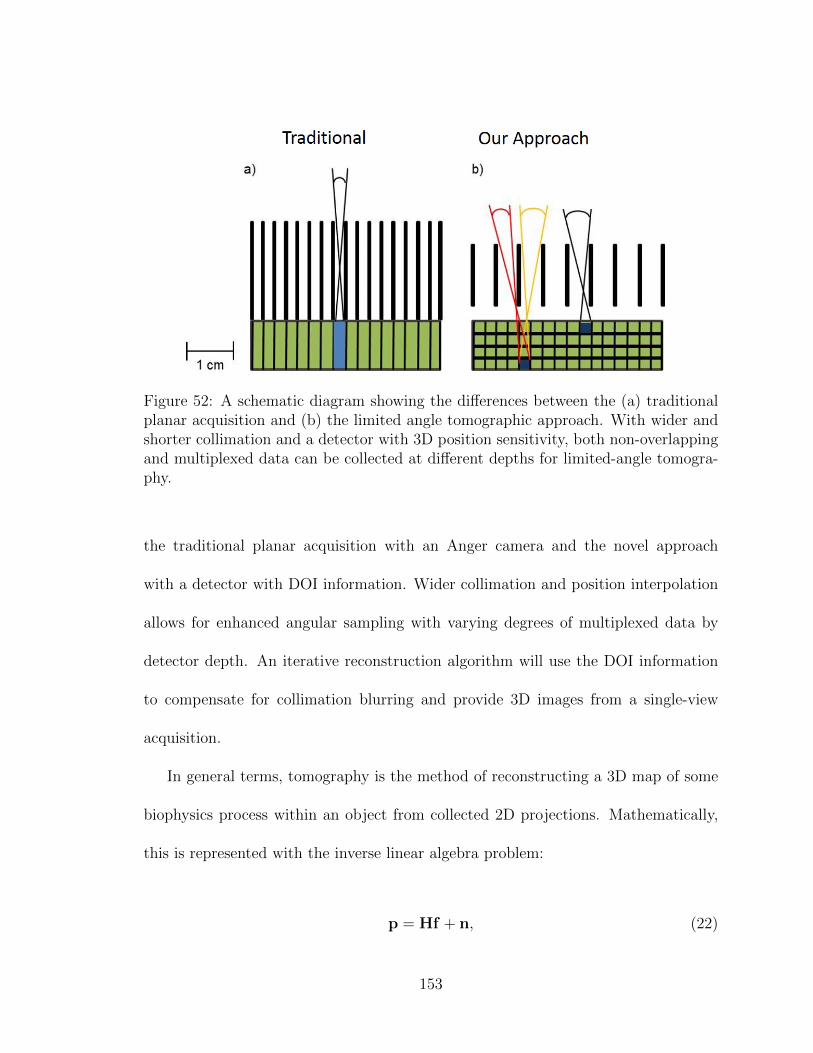
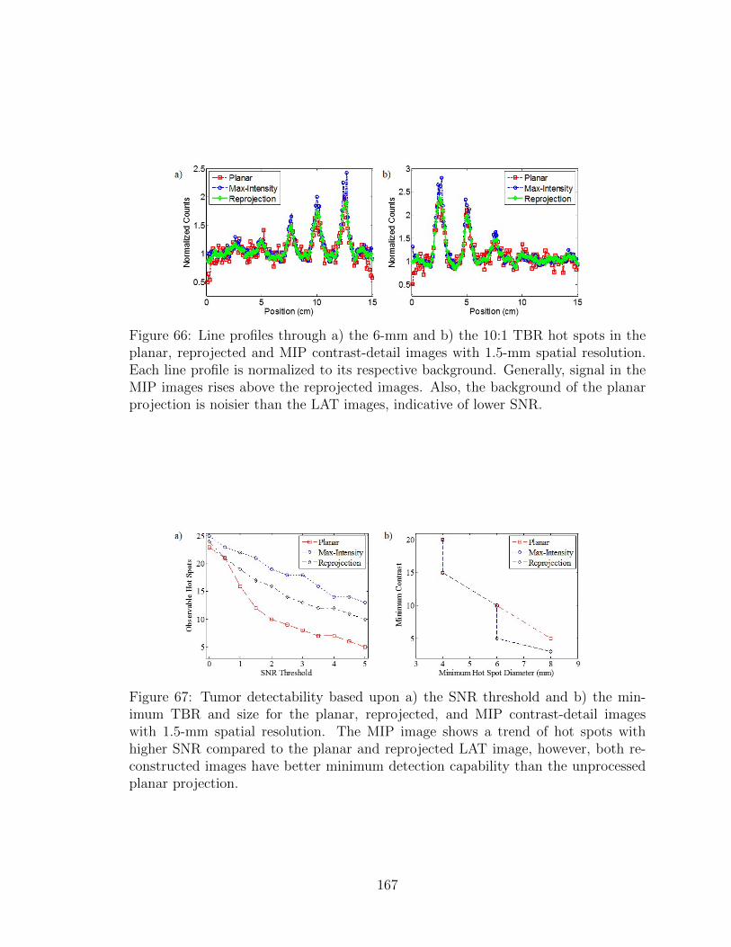
66. Line profiles through the 6-mm and 10:1 TBR hot spots in the pla-nar, reprojected and MIP contrast-detail images with 1.5-mm spatialresolution. . . . . . . . . . . . . . . . . . . . . . . . . . . . . . . . . . 167

67. Tumor detectability based upon SNR and minimum TBR and diameterfor the planar and reconstructed contrast-detail projections with 1.5-mm spatial resolution. . . . . . . . . . . . . . . . . . . . . . . . . . . . 167

68. A schematic diagram of the geometry for the Monte Carlo breast imag-ing simulations with the dual-head HPGe imaging system. . . . . . . . 173

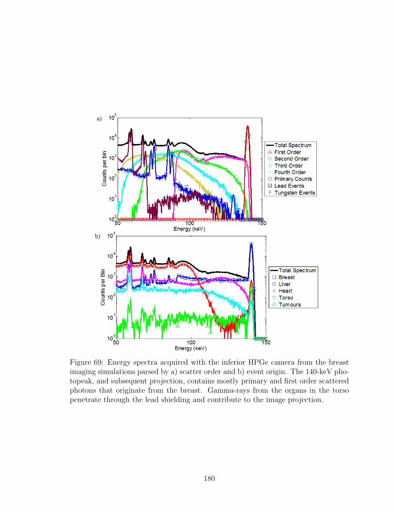
69. Energy spectra acquired with the inferior HPGe camera from the breastimaging simulations. . . . . . . . . . . . . . . . . . . . . . . . . . . . . 180

70. Energy spectra acquired with the superior HPGe camera from thebreast imaging simulations. . . . . . . . . . . . . . . . . . . . . . . . . 181

71. The inferior and superior prefect-resolution projections of the breastphantoms with tumors at depths of 1 cm, 2.25 cm, or 3.5 cm. . . . . . 182

72. Breast images with perfect resolution generated using conjugate count-ing methods. . . . . . . . . . . . . . . . . . . . . . . . . . . . . . . . . 183

73. The NMSE and contrast by iteration curves for the breast images withperfect resolution following OSEM reconstruction. . . . . . . . . . . . 184

74. Reconstructed resolution-free projections of the breast phantom withtumors at varying depths. . . . . . . . . . . . . . . . . . . . . . . . . . 185

xiii

75. Tumor contrast and SNR measurements of hot spots in breast projec-tions with prefect resolution for tumors at varying depths. . . . . . . . 186

76. The inferior and superior breast projections with 1.5-mm spatial reso-lution containing tumors at depths of 1 cm, 2.25 cm, or 3.5 cm. . . . . 187

77. Breast projections with 1.5-mm resolution generated using conjugatecounting methods. . . . . . . . . . . . . . . . . . . . . . . . . . . . . . 189

78. The NMSE and contrast by iteration curves for the breast images with1.5-mm resolution following OSEM reconstruction. . . . . . . . . . . . 190

79. Reconstructed breast projections with 1.5-mm resolution with tumorsat varying depths. . . . . . . . . . . . . . . . . . . . . . . . . . . . . . 191

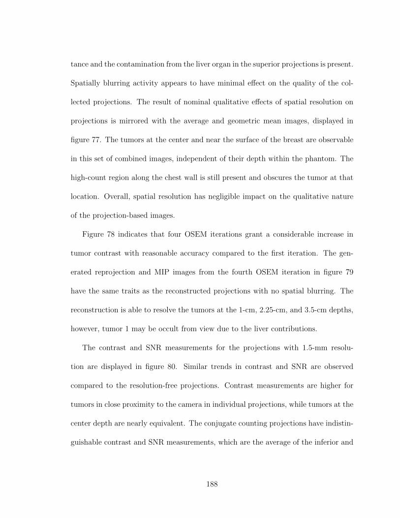
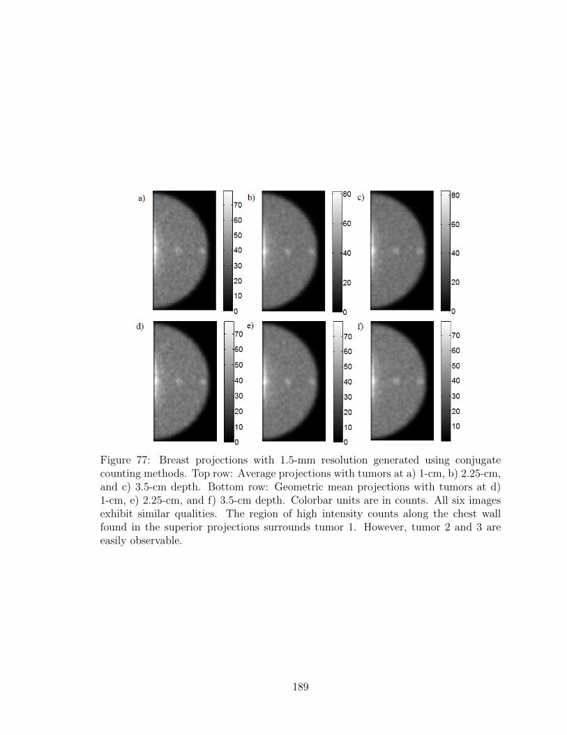
80. Tumor contrast and SNR measurements of hot spots in breast projec-tions with 1.5-mm resolution for tumors at varying depths. . . . . . . 192

81. The NMSE curves for the OSEM reconstructed images with perfectresolution and coronal slices with the lowest NMSE for tumors at the1-cm or 2.25-cm depth. . . . . . . . . . . . . . . . . . . . . . . . . . . 193

82. The contrast-detail projections with perfect spatial resolution for tu-mors at a 1-cm depth. . . . . . . . . . . . . . . . . . . . . . . . . . . . 194

83. The contrast-detail projections with perfect spatial resolution for tu-mors at the center depth of the FOV. . . . . . . . . . . . . . . . . . . 195

84. Tumor detectability curves based upon SNR and minimum TBR anddiameter for the contrast-detail projections with no spatial resolution. 197

85. The NMSE curves for the OSEM reconstructed images with 1.5-mmresolution and coronal slices with the lowest NMSE image for tumorsat a 1-cm or 2.25-cm depth. . . . . . . . . . . . . . . . . . . . . . . . . 198

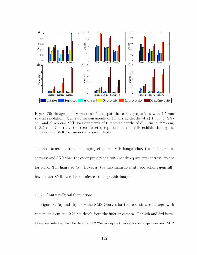
86. The contrast-detail projections with 1.5-mm spatial resolution for tu-mors at a 1-cm depth. . . . . . . . . . . . . . . . . . . . . . . . . . . . 199

87. The contrast-detail projections with 1.5-mm spatial resolution for tu-mors at the center depth of the FOV. . . . . . . . . . . . . . . . . . . 200

88. Tumor detectability curves based upon SNR and minimum TBR anddiameter for the contrast-detail projections with 1.5-mm spatial reso-lution. . . . . . . . . . . . . . . . . . . . . . . . . . . . . . . . . . . . 201

xiv

89. Breast projections acquired by the CZT model and different iterationsof the HPGe model. . . . . . . . . . . . . . . . . . . . . . . . . . . . . 210

90. Measured tumor contrast and SNR from the breast projections gener-ated by different detector models. . . . . . . . . . . . . . . . . . . . . 211

xv

CHAPTER I

INTRODUCTION AND BACKGROUND

The objective of this work is to design and demonstrate the potential imaging

capability of a breast-specific High-Purity Germanium (HPGe) imaging system. Tra-

ditionally, HPGe detectors were used for spectrometry and source identification due

to their superb energy resolution, but the technological challenges of the 1970s limited

biomedical imaging capability. Advancements in amorphous semiconductor contacts,

cryogenics, and readout electronics in the last 40 years have now made HPGe de-

tectors realistic for single-photon imaging. Currently, research with compact HPGe

cameras, fabricated for small-animal imaging, is being conducted; yet extensive work

is needed to determine if HPGe cameras would offer any potential benefit to other

applications.

One application worth exploring is Nuclear Breast Imaging (NBI). The evolution

of NBI has been dictated by the need for improved screening and diagnostic imaging

to better identify disease in women with mammographically dense breast while main-

taining the mammography radiation dose to the patient. Currently, Breast-Specific

Gamma Imaging (BSGI) and Molecular Breast Imaging (MBI) planar acquisition

techniques use specially-designed breast-specific cameras with higher sensitivity and

specificity than screening mammography. MBI employs the state-of-the-art clinical

1

breast imaging system, which utilizes pixellated Cadmium Zinc Telluride (CZT) and

square-hole collimation registered to the pixels for the best spatial resolution and

geometric sensitivity tradeoff. However, the detector capabilities of Germanium de-

tectors have the potential to improve upon breast imaging performance for a few

reasons. The good transport properties of Germanium could overcome the sensitivity

loss due to tailed events observed in CZT. These sensitivity gains would allow for

injecting less of the radiotracer to lower overall radiation dose to the patient. The

energy resolution could suppress scattered events and events originating outside the

field-of-view from degrading image quality. Finally, a Limited-Angle Tomographic

acquisition may be possible with Germanium cameras. Its depth-of-interaction esti-

mation capabilities with mounted wide collimation would grant an HPGe camera a

greater degree of angular sampling around an object without the need of object or

camera rotation. Applying an iterative reconstruction algorithm with the limited-

angle acquisition scheme could result in 3D images with potential enhancements in

contrast and resolution.

To carry out the objective of exploring HPGe-detector potential performance for

NBI, Monte Carlo computational methods will be used to accomplish three specific

aims.

1. To demonstrate the potential benefits Germanium detectors offer to NBI.

2. To develop a breast-specific Germanium imaging system for limited-angle tomog-

raphy.

2

3. To explore the limits of performance for a dual-head limited-angle tomography

HPGe imaging system

The radiation transport package Monte Carlo N-Particle, version 5 (MCNP5) will

be used for all simulations. MCNP5 outputs particle tracking files of position and

photon energies of collisions, which are parsed using MATLAB to retrieve data about

energy deposition and to generate images. Because the computational burden of these

simulations is large, utilizing the campus cluster ACCRE will be essential to expedite

run time.

For aim 1, published findings of simulations modeling a CZT imaging system will

be replicated by generating images with the breast/torso phantom. This system’s per-

formance will be compared against the performance of a generic Germanium system

by substituting the 5-mm CZT for 10-mm HPGe and repeating the measurements.

Experimental characterization and validation of the Germanium camera will be per-

formed and measured system parameters will be incorporated into the HPGe model.

Imaging performance is assessed based on sensitivity (number of absorbed photons),

scatter and torso fractions, and tumor contrast. It is expected that for equivalent

activity imaged, an optimal HPGe breast camera will provide improvements in sen-

sitivity and tumor contrast while better suppressing small-angle scatter events and

background from outside the FOV.

For aim 2, various registered parallel-hole collimators will be evaluated for geome-

3

try sensitivity, resolution and tumor contrast of contrast-detail and breast phantoms.

Limited-angle tomography will be incorporated with the best performing collimator

by generating a system matrix that maps object space to the detector. Applying an

iterative MLEM algorithm will allow previously collected 2D projections with depth

of interaction information to be reconstructed into 3D images. Projections and slices

of the generated 3D images will be compared to the 2D planar images created from

previous simulations and evaluated by tumor contrast and system resolution. It is ex-

pected that the modeled HPGe breast imaging system will provide the advantages of

HPGe detectors observed in aim 1 while providing enhancements in spatial resolution

and tumor contrast due to the addition of tomographic imaging methods.

Finally for aim 3, a dual-head imaging system using two opposing HPGe cameras

will be investigated. Dual-head systems exhibit approximately double system sensi-

tivity over single camera systems and improve spatial resolution close to the second

camera. It has been observed that using opposing dual-head cameras with additional

image processing and analysis can enhance imaging sensitivity as well as the estima-

tion of some tumor properties, including 3D localization and size. Simulations with

opposing HPGe cameras optimized in aim 2 will be conducted to generate planar

images. Applying an OSEM reconstruction with opposing-planar images will provide

tomographic images. It is expected that the combination of depth of interaction infor-

mation from HPGe detectors, attenuation differences between acquired projections,

and application of the OSEM reconstruction algorithm will provide better localization

4

and size of tumors with increased spatial resolution contrast than planar images.

The remainder of the chapter will discuss some essential background for full com-

prehension of this work. Information on biomedical imaging, radiation detectors,

select modalities for breast cancer screening, and the evolution of Germanium detec-

tors will be discussed.

1.1 Radionuclide Imaging Overview

Radionuclide imaging is a biomedical imaging technique designed to acquire the

spatial distribution of a particular biological process of interest. A molecule of in-

terest is labeled with a radioactive atom with a known characteristic emission and

introduced to the subject, usually through injection. The radiotracer is more readily

absorbed where the biological process of interest is occurring at higher rates compared

to other locations within the body. The radioactive atom attached to the molecule of

interest undergoes a radioactive decay process that results in the isotropic emission

of the known characteristic gamma ray. Photons not obstructed or attenuated by the

subject are collected by external gamma cameras. With calibration of the gamma

camera, an energy spectrum of the absorbed photon energies is generated. Placing an

energy window or discriminator for the characteristic energy of emitted photons filters

out scattered or incomplete events, leaving events with full charge collection within

the camera. With position estimation of the energy-filtered events, a projection image

of the radiotracer distribution within the subject can be generated. This information

5

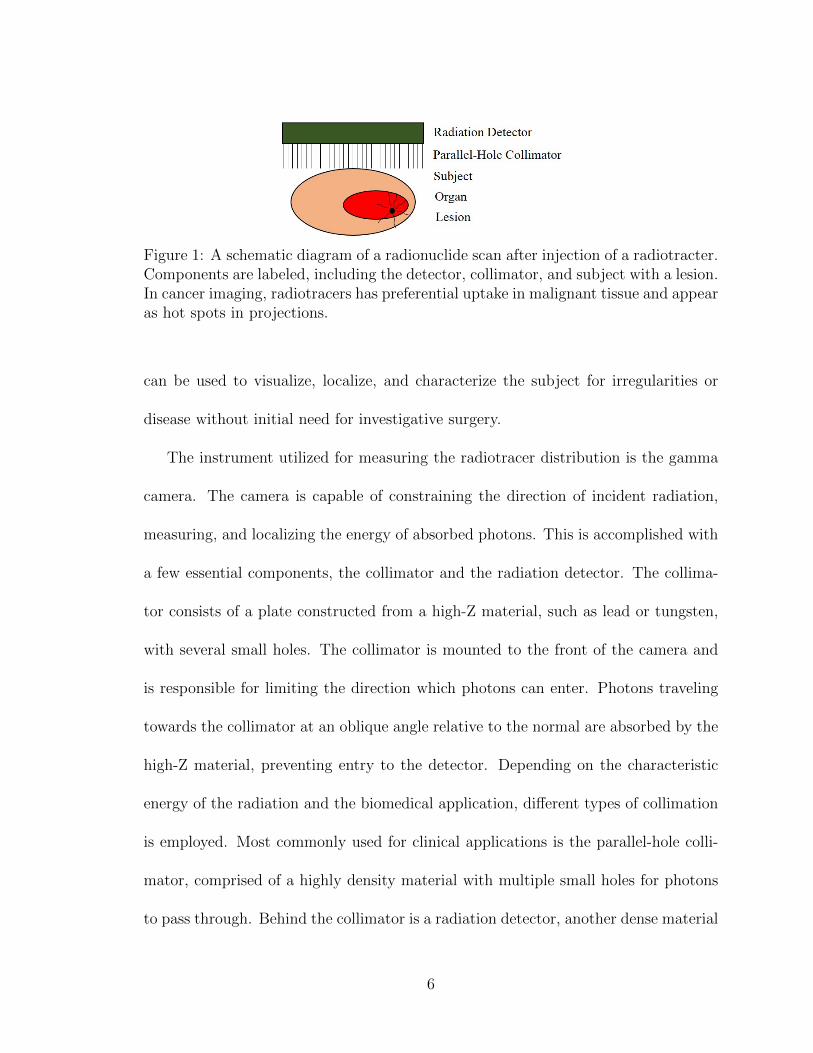
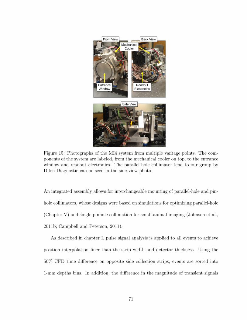
Figure 1: A schematic diagram of a radionuclide scan after injection of a radiotracter.Components are labeled, including the detector, collimator, and subject with a lesion.In cancer imaging, radiotracers has preferential uptake in malignant tissue and appearas hot spots in projections.

can be used to visualize, localize, and characterize the subject for irregularities or

disease without initial need for investigative surgery.

The instrument utilized for measuring the radiotracer distribution is the gamma

camera. The camera is capable of constraining the direction of incident radiation,

measuring, and localizing the energy of absorbed photons. This is accomplished with

a few essential components, the collimator and the radiation detector. The collima-

tor consists of a plate constructed from a high-Z material, such as lead or tungsten,

with several small holes. The collimator is mounted to the front of the camera and

is responsible for limiting the direction which photons can enter. Photons traveling

towards the collimator at an oblique angle relative to the normal are absorbed by the

high-Z material, preventing entry to the detector. Depending on the characteristic

energy of the radiation and the biomedical application, different types of collimation

is employed. Most commonly used for clinical applications is the parallel-hole colli-

mator, comprised of a highly density material with multiple small holes for photons

to pass through. Behind the collimator is a radiation detector, another dense material

6

which absorbs incident photons and converts it into a current pulse. Various radiation

detectors are utilized for radionuclide imaging with gamma cameras, which some of

the most popular are discussed in section 1.2. Some consideration, specifically for

the radiation detector, are the relevant properties that largely dictate gamma camera

performance. These properties are discussed in the following section.

1.1.1 Relevant Imaging Properties

1.1.1.1 Efficiency

An important property of any detector is its sensitivity to radiation, or better

known as its efficiency. The absolute efficiency, which is the ratio of the number

of events recorded to the number of emitted radiation particles, depends on both

characteristics of the detector and the geometry of the system. More widely used

however is the intrinsic efficiency of a detector, also known as the Quantum Detection

Efficiency (QDE), which is defined as the ratio of the number of events recorded to

the number of emitted radiation particles incident on the detector. When primarily

discussing detectors, the intrinsic efficiency is tabulated rather than the absolute

efficiency, as the intrinsic efficiency depends upon the density, electronic density,

stopping power, attenuation coefficient of the material, its thickness and the incident

photon energy (Knoll, 2000; Bushberg and Boone, 2002). The collimator mounted to

the gamma camera also has a geometric efficiency for allowing propagating photons

to pass. This efficiency, also known as sensitivity, for radiation is dependent upon

7

collimator type, material, thickness, and hole dimension. Paralllel-hole collimators

are quite pertinent to clinical gamma cameras, and their geometric efficiency are

discussed more in chapter V.

1.1.1.2 Spatial Resolution

Another important property of a gamma camera is its spatial resolution. Within

the image or detector space, the spatial resolution is the minimum lateral distance

to resolve two distinct hot spots or points. The geometric resolution of the collima-

tor contributes the most to the spatial resolution of an image, on the order of the

collimator pitch. The spatial resolution of the system can be evaluated by acquiring

an image of a point source and measuring the full width at half maximum (FWHM)

of the point spread function (PSF). Single point sources are rare in nature, so line

sources or edge spread functions are acquired instead to measure spatial resolution.

Limits on the intrinsic spatial resolution differ between scintillators and semiconduc-

tor detectors. Pixelated detectors typically have resolution limits on the order of the

detector element size, but energy resolution also influences spatial resolution. Poorer

energy resolution forces utilization of wider energy windows and allows for scattered

events to spread the PSF (Bushberg and Boone, 2002; Cherry et al., 2012; Hendee

and Ritenour, 2003). Energy resolution is discussed further.

8

1.1.1.3 Energy Resolution

An intrinsic property of radiation detectors is the energy resolution; an observable

in detector response distributions. It is a measurement of the spread in a energy

spectrum due to fluctuations in the response of a detector. The energy resolution

is defined as the dimensionless ratio between the FWHM of the photopeak and the

energy of the photopeak. Scintillation detectors have energy resolutions of ∼10% at

140 keV, while semiconductor detectors have superior resolution ranging from 1%-5%

at 140 keV. A general assumption about detector response is that the energy input

is typically linear to its output, which validates the theory that the peak centroid

is proportional to the number of charge carriers created per ionization event. If the

FWHM stays relatively constant, then the energy resolution could be improved with

use of a material that creates more charge carriers per event (Knoll, 2000).

1.2 Radiation Detectors

1.2.1 Scintillators

The technique of observing radiation by the collection of scintillated light created

in materials has been one of the more useful and reliable methods in the study of ra-

diation emission. Scintillation detectors work through a process of converting emitted

radiation into visible light through interactions with an organic or inorganic scintil-

lation material. When radiation interacts with the scintillator, electrons-hole pairs

are created and elevated to higher energy levels. These particles lose some energy

9

through other non-radiative processes and collapse down to activator energy states.

The scintillation light is generated when these electron-hole pairs recombine from

the activator energy states. The emitted scintillator light travels down optical pipes

to photomultiplier tubes (PMT), where the light is converted into photoelectrons at

the cathode. The number of photoelectrons are multiplied through collisions along a

series of dynodes over a variable bias. This avalanche of electrons contributes to the

production of an electrical signal, which undergoes further processing of amplification

and shaping before being collected for analysis (Knoll, 2000; Bushberg and Boone,

2002; Hendee and Ritenour, 2003).

The ideal scintillation detectors hold properties that maximize the efficiency in

converting emitted radiation into the electrical signal. One property of importance

that is unique to scintillator materials is its luminosity, better known as its light yield

or light output. The ideal scintillator would quickly transfer the energy from ionizing

radiation into light with a high efficiency. Also, this conversion of light should be

linearly proportional from the lower energy x-ray to high energy gamma-rays. The

time of the total luminosity should be on the order of nanoseconds for the entire

process of fluorescence and phosphorescence. Highly dense scintillators with high Z

numbers are also favorable for detectors as those materials more readily stop x-rays

and gamma-rays, which leads to shorter attenuation coefficients and higher intrinsic

efficiencies (Bushberg and Boone, 2002).

One of the most popular inorganic scintillators used for radiation detection is

10

Sodium Iodide doped with Thallium as an activator, NaI(Tl). It is considered the gold

standard scintillator material for radiation detector due to its superb light yield and

near linear response over high gamma-ray energies. Because of its superb light yield,

NaI(Tl) also has an excellent energy resolution (∼10% at 140 keV) in comparison

to other inorganic scintillators (Peterson and Furenlid, 2011; Hendee and Ritenour,

2003). Its decay time of 230 ns is average for scintillators, but for use in medical

imaging with high count rates, it is long. In addition, NaI(Tl) undergoes a form

of delayed fluorescence called phosphorescence, which further extends the time of

scintillation within the crystal and limits the timing capability of NaI(Tl) detectors.

It is also a very delicate material that cracks easily and absorbs moisture from the air,

making encasement necessary. Even with some of its shortcomings, it is inexpensive

to produce, and thus has been the basis for the Anger Camera, the clinical standard

for gamma cameras and nuclear medical devices systems (Knoll, 2000; Bushberg and

Boone, 2002).

Table 1 lists the properties of select scintillator crystals used for nuclear medicine

and other applications. A considerable amount of work has been accomplished with

CsI(Tl) and La-based scintillators due to their high light yield, which translates into

good energy resolution. A novel scintillator, SrI2, has emerged as a suitable can-

didate for potential imaging application with high light yield, but decay times are

uncomfortably slow for high count rate acquisitions.

11

Table 1: Properties of select scintillators. Table information acquired from Petersonand Furenlid (2011); Van Loef et al. (2009).

Density Attenuation Coe. MaximumDecay Time (ns)

Light Yield(g/cm3) at 140 keV (cm-1) Emission (nm) (photons/keV)

NaI(Tl) 3.67 3.12 415 230 38CsI(Tl) 4.51 4.53 540 680 (63%), 3340 (37%) 65

LaCl3(Ce) 3.86 2.82 330 20 (70%), 213 (30%) 49LaBr3(Ce) 5.30 3.42 358 35 (90%) 61SrI2(Eu) 4.59 - 435 1110 80

1.2.2 Semiconductors

Semiconductor diode detectors hold great advantages over scintillation crystals

due to their superior energy resolution from the larger number of charge carriers pro-

duced per ionization event. Because of the process of converting ionization energy

into an electric signal for scintillation detectors, energy on the order of 100 eV is

required to produce a charge carrier. However, because semiconductors are able to

directly convert ionizing radiation into an electrical signal, only a few eV, depending

on the semiconductor, is necessary to create an electron-hole pair. As the energy

requirements for producing charge carriers in semiconductors is much lower than in

scintillators, radiation of certain energy will yield more charge carriers in semicon-

ductors than in scintillators. This increase in charge carriers allows for the reduction

in statistical fluctuations and improves upon energy resolution. Semiconductor diode

detectors are also compact in size and have relatively fast timing properties that allow

for the process of pulses in high count rates scenarios.

Semiconductor detectors work on the effects of doping them with materials with

one more valence electron (n-type) and one fewer valence electron (p-type). The

12

addition of these impurities in the semiconductor growth process will form a semi-

conductor junction with an imbalance of electrons and holes; holes being the absence

of electrons. This region is known as the depletion region, which can absorb radi-

ation. The charge imbalance of electrons and holes in the depletion region yields a

small potential (ψ) that satisfies Poisson’s equation:

∇2ψ = − ρ

ε, (1)

where ρ is the volumetric charge density and ε is the dielectric constant of the semicon-

ductor. With a reverse bias applied to the semiconductor, the negative and positive

ions travel away from the junction and increase the width of the depletion region.

This can be seen from the voltage dependence on the width of the depletion region

in (2):

d =

√2V ε

eN. (2)

Thus, applying an appropriate voltage that extends the depletion region throughout

the thickness of the semiconductor maximizes the active volume of the detector and

provides the highest possible efficiency for ionizing radiation.

There are a few important relevant properties of semiconductor diode detectors.

The energy gap between the valence and conduction band, the band gap, is the most

predominant of properties for the semiconductor. For a material to be considered

a semiconductor, its band gap must be small enough, on the order of a few eV,

13

to allow for thermal excitation of electrons. This gives semiconductors their high

conductivity over insulators. The probability of thermally generated electron-hole

pairs in semiconductors heavily depends on the ratio of the band gap energy and the

operation temperature of the detector. For some semiconductor detectors, such as

Germanium, this property creates a necessity to operate them at 70 K to minimize

the number of thermally excited ions. However, this is not the case for Cadmium

Zinc Telluride or Silicon detectors.

The applied electric field in a semiconductor diode detector heavily affects the

migrating of negative and positive charges towards the electrodes for collection. The

net drift velocity of both the electrons and holes are linearly proportional to the

magnitude of the electric field by the mobility of that particle. In most semicon-

ductors, the electron- and hole-mobilities are roughly similar, so collection times for

the electrons and holes are also similar, on the order of tens of nanoseconds. At

higher electric fields, the drift velocity eventually reaches a saturation point, where

increasing the electric field ceases to increase the net drift velocity. For fast detection,

semiconductor diodes are operated at applied electric fields that allow for this drift

velocity saturation, which allow for quick collection times. Diffusion of charge also

affects the collection time, as charge will drift down longer paths while approaching

the anode and cathode, slightly increasing the collection time and altering position

measurements. These effects are minimal in small volume detectors, but cause signif-

icant changes in timing and position measurements in large volume detectors (Knoll,

14

Table 2: Properties of select semiconductor. Table information adopted from Petersonand Furenlid (2011).

Mobility-LifetimeDensity Attenuation Coe. Energy per Electron Hole(g/cm3 at 140 keV (cm-1) e-h pair (eV) (cm2/V) (cm2/V)

Si 2.33 0.02 3.61 0.42 0.22Ge 5.32 0.72 2.98 0.72 0.84

CZT 5.82 3.07 5.0 3× 10−3 5× 10−5

2000).

Trapping and recombination effects due to the presence of impurities can also

affect the total collection of charge and worsen energy resolution. Electrons and holes

can be captured by impurities that contain energy states in between the valence and

conduction bands. In one case of trapping effects, these charge carriers are trapped

and released, but after the measurement of the pulse. In the case of recombination,

an electron and hole recombine and annihilate in the region of an impurity. There

can be also structural defects, such as point or line defects, in the semiconductor that

can contribute to trapping and recombination. These combined effects contribute to

the loss of charge and can cause a decrease in the measurement of the true energy of

x-rays and gamma-rays. This in turn can negatively affect the energy resolution of

the detector (Knoll, 2000; Barber, 1996)

Table 2 lists the properties of select semiconductors used for nuclear imaging. Sili-

con is an appropriate detector for x-ray, CT, and low energy gamma-ray applications,

but is not directly applicable to the work of this document. CZT and HPGe are

discussed in greater detail in the following sections.

15

1.2.2.1 Cadmium Zinc Telluride

Cadmium Zinc Telluride, a compound material of Zinc Telluride and Cadmium

Telluride, is a popular room temperature semiconductor. CZT is a highly dense

material with a density of 6.2 g/cm3. Its band gap energies can range from 1.53 eV to

1.64 eV, depending on the ZnTe and CdTe concentrations. Electron mobility is much

better at 1350 cm2/Vs than its hole mobility at 120 cm2/Vs. CZT has a measured

energy resolution as good as 1.7% at 662 keV and ionization energy of 5.0 eV per

electron-hole pair (Knoll, 2000). These properties allow for more compact systems

with superior energy resolution at room temperature than NaI(Tl) scintillators.

However, CZT suffers from charge carrier transport issues and has high industrial

costs. Improvements have been made through designing different detector geometries

and additional signaling processing with added electronics to account for the poor

hole transport, however, it is unclear if these improvements would work with large

volume detector-arrays. Energy resolution for CZT detectors has been shown to

be superior to most scintillators. Even with better resolution, spectra of CZT can

comprise of long tails that span to the low energy side of the photo peak. This

effect is caused by charge carrier trapping, pixel non-uniformity in charge collection

between the center and boundaries of the pixel, and the slow drift velocity of holes.

The low energy tailing effect can be mitigated by utilizing small pixels sizes in CZT

detector systems. The weighting potential strength near the small contacts with

preferential absorption of gamma rays allows for only negative charge carriers to

16

contribute to signal generation and removes the influence of hole drifting. Adding

collimator walls around the individual pixels to shield against boundary and pixel

sharing effects also improves spectral quality (Wagenaar, 2004; Barrett et al., 1995;

Bolotnikov et al., 2005). Arrays of 3D position-sensitive pixilated CZT spectrometers

have been developed using Application Specific Integration Circuit (ASIC) readout

systems that integrate the energy and timing circuits into a single chipset, but the

spectrometers still suffer from variations in electron trapping, electronic noise, non-

linearity and nonuniformity between pixels (Zhang et al., 2004, 2005).

1.2.2.2 Germanium

Germanium (Ge) is another semiconductor material with major use in several

disciplines requiring gamma-ray spectroscopy. Originally grown using lithium drift

methods as Ge(Li) (read:Jelly) detectors, the development of zone refinement tech-

niques led to ultrahigh purity Germanium, known as HPGe. Ge has a moderate

density of 5.32 g/cm3 with a low bandgap of 0.665 eV at 300 K. The mobilities of

electrons and holes in Germanium at room temperature are superior to CZT with

values of 3900 and 1900 cm2/Vs. However, the low bandgap of Germanium results in

thermal excitations of charge-carriers, making Ge detectors nonoperational at room

temperature. For this reason, traditional Ge detectors are cooled using liquid nitro-

gen or other refrigeration methods to 77 K. This improves Germanium performance

by increasing the mobility of charge-carriers to 3.6×104 and 4.2×104 cm2/Vs for elec-

17

trons and holes, respectively. Combined with generating 2.96 electron-hole pairs per

eV absorbed, Germanium yields the best energy resolution of any radiation detector

at <1% at 140 keV (Knoll, 2000; Johnson et al., 2011a). The challenges of keeping

HPGe detectors at liquid nitrogen temperatures hindered their development. How-

ever, attempts at fabricating and evaluating HPGe gamma cameras have been made

in past and are highlighted in section 1.3.

1.3 Germanium Gamma Camera History

Original designs for Germanium detectors included orthogonal strip contacts on

monolithic slabs of germanium for position sensitivity. One of the first position sensi-

tive HPGe detectors was first tested in the 1960s. J. F. Detko evaluated a 20 mm ×

20 mm × 10 mm orthogonal-strip HPGe in the late 1960s. The system had a 3.27%

energy resolution at 122 keV and a measured spatial resolution of 3 mm (Detko,

1969). Several other HPGe detectors were evaluated by other groups for spatial and

energy resolution, including a detector with a 2 cm × 2 cm area and a thickness of

10 mm. Typical spatial and energy resolutions measured with these detectors were

between 2.2-4.0 mm and 2.5% @ 140 keV on average, respectively (Schlosser et al.,

1974).

These properties were attractive for nuclear medicine, so work towards a clini-

cal system was pursued. The first clinical tests on a prototype gamma-camera were

constructed from lithium-drifted germanium that was 44 mm × 44 mm in area and

18

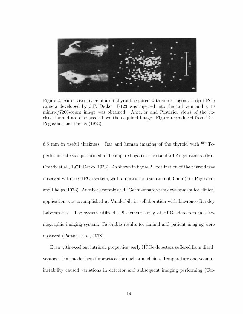
Figure 2: An in-vivo image of a rat thyroid acquired with an orthogonal-strip HPGecamera developed by J.F. Detko. I-123 was injected into the tail vein and a 10minute/7200-count image was obtained. Anterior and Posterior views of the ex-cised thyroid are displayed above the acquired image. Figure reproduced from Ter-Pogossian and Phelps (1973).

6.5 mm in useful thickness. Rat and human imaging of the thyroid with 99mTc-

pertechnetate was performed and compared against the standard Anger camera (Mc-

Cready et al., 1971; Detko, 1973). As shown in figure 2, localization of the thyroid was

observed with the HPGe system, with an intrinsic resolution of 3 mm (Ter-Pogossian

and Phelps, 1973). Another example of HPGe imaging system development for clinical

application was accomplished at Vanderbilt in collaboration with Lawrence Berkley

Laboratories. The system utilized a 9 element array of HPGe detectors in a to-

mographic imaging system. Favorable results for animal and patient imaging were

observed (Patton et al., 1978).

Even with excellent intrinsic properties, early HPGe detectors suffered from disad-

vantages that made them impractical for nuclear medicine. Temperature and vacuum

instability caused variations in detector and subsequent imaging performing (Ter-

19

Pogossian and Phelps, 1973). These designs used diffused dopant contacts, which

were required to sit within cut channels in the detector material to reduce capaci-

tance effects between electrodes and impaired detector efficiency. Also sorting out

multiple-hit events was difficult and often worsened energy resolution. These diffi-

culties halted the development of HPGe cameras for medical imaging applications

(Barber, 1996).

During the mid-90s and through the turn of the century, amorphous-semiconductor

contacts for Germanium detectors were further developed from work completed in

the 1970s (Luke et al., 2000; Hansen and Haller, 1977). The fabrication of these new

contacts is described as a simple process which provides finer pitch electrodes than

diffused Lithium metal contacts (Luke et al., 2000). These new contacts have led

to the development of prototype position-sensitive germanium detectors for imaging

applications in many fields (Amman and Luke, 2000).

The process for obtaining position information from orthogonal strip detectors is

through pulse shape analysis of signal waveforms, shown in figure 3. The electron-

hole pairs generated from absorbed photons induce full signals on the collecting strips.

However, the induction of short-lived transient signals on adjacent neighboring strips

are also generated during charge carrier travel towards the collecting strips. Using a

posteriori knowledge of the ratio between the difference in the maximum or integral

of these transient signals and the deposited energy, position estimation and spatial

resolutions finer than the physical width of the strips can be achieved. Depth in-

20

Figure 3: An example waveform characterizing a single event absorbed in a double-sided strip Germanium detector. Full charge collection over a set of orthogonal stripsforms the large amplitude signals, while charge-carrier motion through electrode po-tential induces transient signals on neighboring strips. Real charge is not collect onneighboring strips, resulting in the quick rise and fall of transient signal. Ratios ofthe transient signals are used for inter-strip interpolation. Figure reproduced fromVetter et al. (2004).

21

formation of photonic interactions can be gathered from the difference in the time

of max signal from charge-carrier collection. Pulse shape analysis of collected signal

waveforms ultimately enables position sensitivity in all three dimensions (Burks et al.,

2004; Vetter et al., 2004).

A disadvantage to double-sided strip detectors is their gaps between the strips.

While wider gaps can decrease capacitance between strips, the additional space can

lead to the trapping of charge-carriers and eventual charge loss. Events that undergo

charge loss are typically deemed unusable and are excluded. Moreover, Compton

events that propagate to adjacent strips or lead to trapped charge-carriers in gaps

are excluded from processing, ultimately decreasing detection efficiency. A significant

amount of work to correct for charge loss due to gaps has been accomplished by

Hayward and Wehe (2007, 2008a,b). They found that interactions that occur within

the gap are complicated by: (1) incomplete charge collection; (2) signal variance due

to charge-carrier cloud size and motion; (3) distinguishing between single interactions

and multiple close interactions to the gap. Haywood and Wehe developed correction

methods for single site interactions and close Compton events depend on the measured

energy from the adjacent strips.

Others have also explored the use of HPGe detectors as imaging cameras. One

study modeled and compared the performance between a Germanium Orthogonal

Strip Detector (GOSD) and an Anger camera with NaI(Tl) scintillation crystals in a

simulated breast study. Their results suggest that GOSD will provide better contrast,

22

SNR and superior spatial resolution with a small sacrifice in sensitivity. However, the

superior energy resolution of Germanium compensates for its relatively modest linear

attenuation coefficient and offers moderate sensitivity compared to the Anger camera

(Gombia et al., 2002).

A group at the University of Liverpool has been exploring the use of Germa-

nium detectors for pre-clinical and other imaging applications. The Small Animal

Reconstruction Tomography for Positron Emission Tomography (SmartPET) system

was developed originally as a proof of principle by using two 20 mm thick HPGe

detectors to measure coincident 511 keV events of 22Na sources. The study lead to

the advancement of event categorization using pulse shape analysis to determine the

order of interactions in each detector. Even with decent energy and spatial resolu-

tion, sensitivity measurements were poor for 511 keV photons (Cooper et al., 2009).

The Liverpool group has explored using the SmartPET system for Compton imag-

ing, which has improved sensitivity for SPECT radionuclide photon energies. The

system may best be optimized when HPGe is used as the scattering detector or as

the analyzing detector (Harkness et al., 2009).

1.4 Breast Cancer Imaging

1.4.1 X-Ray Mammography

Mammography is a radiographic examination that is specialized for detecting

breast tumors. For over 60 years, mammography has been the medical standard for

23

breast imaging for the screening of breast cancer. Although the technique of mam-

mography has not changed since the mid-1950s, several technologic components have

seen advancements and improvements for better contrast and detail. X-ray mammog-

raphy takes advantage of the differences between healthy tissue and cancerous tissue

in the breast. X-rays are sensitive to the changes in electron density of these tissues,

causing linear attenuation differences across the range of x-rays energies. Bombard-

ing x-rays through the breast to analog or digital film produces a planar image of

the attenuation differences, where microcalcifications or other irregularities can be

identified (Bushberg and Boone, 2002).

There are several advantages that make mammography the current standard for

breast imaging. It has a low cost and is widely available across the globe. Using x-ray

mammography, many trained medical professionals are able to deduce and identify

whether a patient is positive for tumors and its level of malignancy or benignancy.

This yields to a high sensitivity percentage of correctly identifying cancers. Most

importantly, mammography delivers a very low dosage of radiation to the body. In a

recent study comparing the absorbed dose in different nuclear breast imaging modal-

ities, the cumulative radiation dose associated with annual screening mammography

in women between 40 and 80 years young was estimated to induce 20-25 cases of can-

cer per 100,000 patients. Mammography is the only technique that has been proven

to lower the risk of terminal breast cancer in women (Hendrick, 2010).

However, mammography is greatly limited in a sub-section of women with dense

24

breast tissue. In these mammographically dense breast patients, the rate of false-

negatives (the misdiagnosis of no cancer when breast tumors are actually present)

increases, causing sensitivity to fall off considerably. Furthermore, the specificity, or

the ability to accurately detect the presence of no cancer or detect benign tumors,

is said to be very low in mammography. This is due to the lack of metabolic or

functional information from mammograms (Rosenberg et al., 1998). Because the

detection of cancer can be poor or inconclusive, an increase of biopsies, a very invasive

procedure that involves removing living tissue to test for the presence of disease, is

seen. Avoiding unnecessary biopsy procedures with severe complications in the case

of false-positive cases (when a cancer diagnosis is given for a healthy patient) can

lower hospital cost, patient cost, and save the patient a load of grief. At the core

of the problem, medical professionals and their patients require novel breast imaging

techniques that will better allow them to identify disease.

This has been the motivation for the improvements made in the technology and

techniques of breast imaging. There is a plethora of breast imaging techniques that

have been developed and seen success in the clinical realm. Many of these modalities

are outside the scope of this paper, as its focus is the development of radiation de-

tectors for the measurement of single-photon emitting tracers. The following section

will briefly highlight alternative breast imaging techniques and how they compare to

mammography.

25

1.4.2 Alternative Imaging Modalities

1.4.2.1 Ultrasonography

Ultrasonography (US) is an ultrasound based technique used to non-invasively

visualize internal structures of the body. When first applied to breast imaging in the

mid-1960s, it was referred to as ultrasound mammography. Ultrasound works through

the emission and absorption of sound waves that propagate through the body and

interact at the boundary of regions with varying density and acoustic properties.

Collection of these reflected waves is used in the reconstruction of an image.

Advantages to breast ultrasonography are its ability to image with decent spatial

resolution and sensitivity with the lack of ionizing radiation dose to the patient. How-

ever, there is a trade-off between the resolution and the depth which one can image

with US. Original work with ultrasonography of breast found that it is more sensitive

than screening mammography, but that there are still issues with diagnosing false pos-

itives due to the lack of specificity of sound waves to determine malignancy (Baum,

1977; Warwick et al., 1988). Because of this, breast ultrasonography is presently

considered a diagnostic tool that can be employed after screening mammography has

been done (Silverstein et al., 2005).

1.4.2.2 Magnetic Resonance Imaging

Magnetic Resonance Imaging (MRI) is another technique used for breast cancer

screening and diagnostic imaging. Instead of using ionizing radiation like mammogra-

26

phy and other nuclear breast imaging techniques, MRI uses magnetic fields and radio

waves to manipulate nuclear magnetization to visualize internal structures with good

spatial resolution and tissue contrast.

MRI has been investigated as a tool for the screening of women with mammo-

graphically dense breasts who have a genetic predisposition to cancer. One study

showed that in women with a high cumulative lifetime risk for cancer, MRI had a

sensitivity of 79.5%, which was more than twice as sensitive as mammography at

33.3% (Kriege et al., 2004). With MRIs superior sensitivity over mammography,

another study continued screening at-risk patients and evaluated tumor progression

and prognosis against a similar group of patients screened with mammography. MRI

discovered smaller, less advance-staged breast tumors than conventional x-ray mam-

mography, and as a result, reduced incidences of late stage tumors by 70% (Warner

et al., 2011). Despite evidence that MRI is less specific than other modalities, includ-

ing mammography, use of MRI screenings enables better differentiation capability of

cancer than mammography (Kriege et al., 2004).

1.4.2.3 Positron Emission Mammography

Positron Emission Mammography (PEM) uses the technology of position emis-

sion tomography (PET) to acquire tomographic images of the biodistribution of 18F-

Fludeoxyglucose (FDG), a glucose derivative highly absorbed in malignant tumors.

Early designs of PEM systems used various highly dense, high Z scintillators such

27

as Bismuth Germanate (BGO) and Gadolinium Oxyorthosilicate (GSO) as planar

detectors. Characterization of these systems using breast phantom with simulated

tumors revealed this technique’s advantages. Overall, the systems are very sensi-

tive and specific to cancerous tissues with spatial resolutions down to 2 - 4 mm.

When light compression of the breast is applied, as opposed to standard prone or

supine positions, detectability of lesions increases such that 5 mm tumors were visi-

ble (Thompson et al., 1995; Raylman et al., 2000). When a BGO PEM system was

first brought to clinical trials with a small number of subjects, 86% sensitivity and

100% specificity were found (Murthy et al., 2000).

Observations of PEMs limitation were the amount of Compton scatter events

recorded (∼12% of events), which only increased as the breast density increased. In-

creases in breast density also caused a decrease in minimum tumor size detectability to

the point where tumors less than 1 cm in diameter were not visible. Furthermore, the

radiation dose involved in PEM has a 20 times higher fatal radiation-induced cancer

risk than screening mammography for women of age 40 and above (Hendrick, 2010).

Absorbed doses can be diminished with better radiation detectors with improved

efficiency, such as Lutetium Oxyorthosilicate (LSO) or even semiconductors, which

would produce images of similar quality with less injected radioactivity. Consensus

among medical professionals states that even though PEM has similar sensitivity and

slightly improved specificity to breast MRI, dose and risk concerns make it an ade-

quate adjunct to mammography only when MRI is unavailable or gives contradicting

28

results from other modalities (Silverstein et al., 2005).

1.4.3 Nuclear Breast Imaging Methods

Nuclear Breast Imaging (NBI) is an umbrella term that is used to encompass

breast imaging modalities that utilize internalized radiopharmaceuticals that emit

high energy gamma-ray radiation and is measured and localized using solid state

detectors. In the following section, the evolution of NBI is outlined with its own

advantages over screening mammography and its current limitations as an imaging

technique.

1.4.3.1 Scintimammography

Scintimammography is best described as breast-specific scintigraphy, where radionuclide-

labeled tracers are injected and more readily absorbed in cancerous tissue than healthy

tissue. Scans are performed by having patients lay on a bed in a prone position with

general-purpose or whole-body gamma cameras that acquire planar images, an exam-

ple of which appears in figure 4. The radiopharmaceutical Technetium-99m sestamibi

(99mTc-MIBI), originally a pharmaceutical for investigating cardiac dynamics, is in-

jected as a tracer for tumors. This system and procedure allows for planar images of

each breast to be taken in similar projections to complement screening mammography

(Khalkhali et al., 1999).

When 99mTc-MIBI was found to be a suitable radiotracer for the identification of

29

Figure 4: Photograph of a woman undergoing a conventional scintimammographyscan using general-purpose cameras. The patient lies in a prone position with camerasimaging laterally from the body. Photo reproduced from www.imaginis.com.

cancer, several centers studied its usefulness in the detection of breast cancer as a

complement to screening mammography. Methods for prone imaging of breast were

followed in many studies that compared screening mammography and scintimam-

mography. Khalkhali found that in a study of 147 women with 153 breast lesions,

his scintimammography techniques were able to detect 92.2% of the malignant tu-

mors accurately (sensitivity) and 89.2% of the benign tumors accurately (specificity)

(Khalkhali et al., 1995). Studies conducted in other centers across the globe (Canada,

Spain, and Texas, USA) using Khalkhali’s method for prone imaging found very simi-

lar results in the performance of scintimammography. Over the course of these studies,

the sensitivity to detecting malignant tumors for scintimammography ranged between

83% and 92%, while specificity of benign tumor detection had a wider range of 79%

to 94% (Taillefer et al., 1995; Villanueva-Meyer et al., 1996; Prats et al., 1999). Ex-

amples of collected images are displayed in figure 5. In many of the studies, patients

30

Figure 5: a) A mammogram presents with a malignant mass and architectural distor-tion with possible metastases at the lymph node. b) The same breast acquired usingscintimammography. Black arrows correlate to cancer masses and white arrows pointto axillary lymph node involvement. Images reproduced from Prats et al. (1999).

were selected based on mammograms that showed inconclusive or abnormal results,

which is a common occurrence in at-risk women with dense breast tissue.

Scintimammography has a couple of advantages over standard x-ray mammogra-

phy. Most importantly, the technique is independent of breast density due to the use

of high energy gamma rays that are better able to penetrate through tissue. The

interference patterns observed in standard mammography often shield small breast

tumors that go undetected, worsening sensitivity and specificity. As such, scintimam-

mography’s sensitivity and specificity are superior to mammography. In the case of

indeterminate or inconclusive mammograms, scintimammography is another tech-

nique better able to detect the presence of malignant cancers rather than pursuing

invasive biopsies.

However, scintimammography also exhibits its own set of limitations. The major

reason for its limitations is inherent to the cameras and the camera position during

31

imaging acquisition. The spatial resolution of the imaging system deteriorates due

to the distance between the camera and the object. Along with the degradation of

spatial resolution, the general-purpose cameras, designed for whole body imaging,

have a large field-of-view. This large FOV can see much of the background from the

torso, including hot regions like the heart and liver, which can further blur images.

Conclusions of studies comparing mammography to scintimammography reference

that cameras with smaller FOVs that center on the breast and chest wall with high

resolution could improve imaging performance Khalkhali et al. (1995); Taillefer et al.

(1995); Villanueva-Meyer et al. (1996); Prats et al. (1999). This need for breast-

specific cameras drove many of the advances in NBI during the turn of the millennium.

1.4.3.2 Breast Specific Gamma Imaging

Breast-Specific Gamma Imaging (BSGI) is a technique currently commercialized

by Dilion Technologies (Newport News, VA). Similar to scintimammography, BSGI

uses a radiotracer, specifically 99mTc-MIBI. The key advantage to BSGI over scin-

timammography is the use of specific radiation detection cameras that have been

optimized for the breast (Majewski et al., 2001; Kieper et al., 2003; Garibaldi et al.,

2006). These breast specific cameras sit much closer to the body in similar fash-

ion to mammography systems, thus recovering much of the sensitivity and spatial

resolution lost in scintimammography. The imaging geometry in practice is shown

in figure 6. With light compression applied, short lesion-to-detector distances can

32

Figure 6: A photograph of a woman undergoing a BSGI scan using the Dilon 6800system. Photo reproduced from Dilon Diagnostics at www.dilon.com.

improve image quality while acquiring projections similar to those of mammography.

The small field-of-view cameras in BSGI also employ the scintillation detector tech-

nology described for scintimammography. However, BSGI cameras employ multiple

10 mm thick NaI(Tl) crystals that are separated by thin reflective septa. This pixel-

based scintillation camera approach does not suffer from edge effects as the monolithic

crystals used in general-purpose cameras (Brem et al., 2002).

Patient studies using breast-specific cameras have quoted higher sensitivity for

detecting breast cancer over other imaging modalities. In the pilot study of a BSGI

system, 50 patients with 58 tumors were scanned for breast cancers with both general-

purpose cameras and an array of 3 mm × 3 mm × 10 mm NaI(Tl) crystals optically

coupled to position-sensitive PMTs, referred to as High-Resolution Breast-specific

Gamma Camera (HRBGC). Results of the study found that the HRBGC outper-

formed the scintimammography camera by detecting 78.6% (22/28) of all malignant

tumors versus 64.3% (18/28) with equal specificity for benign tumors. The salient

33

Figure 7: Comparable images of the same patient with mammography and BSGI.BSGI is capable of localizing high metabolic activity, providing clearer visualizationof potential disease than standard mammography. Photos reproduced from DilonDiagnostics at www.dilon.com.

point made in the study was that the HRBGC found 4 tumors less than 1-cm in di-

ameter that were left undetected by the general purpose camera (Brem et al., 2002).

In other patient studies, the BSGI systems of Dilon Technologies were used as

adjunct modalities in the determination of benign and malignant breast tumors. In

2005, a study was released where 94 high risk women between the ages of 36 and

78 years young with normal mammograms underwent scintimammographic exams.

Those who had abnormal results from BSGI had cancer confirmed with ultrasonog-

raphy (US) or biopsy. Results showed that 16 women with normal mammograms

had some abnormal finding. In 14 of those cases, findings of benign tumors were

confirmed with US or biopsy, while two cases had invasive carcinoma under 1 cm

in size diagnosed with US-guide biopsy (Brem et al., 2005). A retrospective review

of 146 women undergoing BSGI and biopsy has also been performed. Out of 167

lesions, BSGI detected 80 out of 83 malignant tumors for a sensitivity of 96.4%. Of

the other 84 benign tumors, BSGI confirmed 50 of them for a specificity of 59.5%.

34

However, even with high sensitivity and moderate specificity, approximately 30% of

abnormal results were false positives and 3 (∼5%) true negatives were not detected.

Of great importance, BSGI accurately identified 16 of 18 cancers under 1 cm in di-

ameter. Thus, an argument can be made that using breast specific gamma cameras

can detect early stage cancers with high sensitivity (Brem et al., 2008).

The performance of the cameras of BSGI is intrinsically limited by the perfor-

mance of scintillation crystals. NaI(Tl) has been the industry standard for radiation

detection, however, its properties are not ideal for medical imaging. One disadvantage

of NaI(Tl) is its fluorescence time of approximately 230 nanoseconds, which limits the

level of radioactivity that can be measured. Another limitation in scintillator perfor-

mance is the process of converting optical photons to a measurable electrical signal.

On average in scintillators, 100 eV is required to create a single charge carrier. In ad-

dition, the poor light collection yield of the PMT can play a role in the degradation of

energy resolution. Ultimately, these processes limit the energy resolution of NaI(Tl).

A general assumption about detector response is that the energy input is typically

linear to its output, which validates the theory that the peak centroid is proportional

to the number of charge carriers created per ionization event. If the FWHM stays

relatively constant, then the energy resolution could be improved with use of a ma-

terial that creates more charge carriers per event (Ter-Pogossian and Phelps, 1973;

Knoll, 2000).

35

Figure 8: A photograph of the MBI dual-head system, the LumaGem 3200S, whichutilizes CZT detectors. Photo reproduced from Hruska et al. (2008).

1.4.3.3 Molecular Breast Imaging

Molecular Breast Imaging (MBI) is another NBI technique whose investigation

is led by the Mayo Clinic. It is currently marketed not as a replacement for x-ray

mammography, but as a diagnostic technique when mammograms are inconclusive.

MBI utilizes dedicated small field of view gamma cameras for detecting breast cancer.

The design and technology used in MBI is very similar to the techniques of BSGI,

however, MBI employs the room-temperature semiconductor Cadmium Zinc Telluride

crystals instead of conventional scintillation crystals. An example of a modern MBI

system is the LumaGem 3200S, shown in figure 8.

The initial question that the Mayo Clinic addressed was the role of energy reso-

lution for NBI. As previously stated, semiconductors have superior energy resolution

over scintillators, but does the improvement in energy resolution truly translate into

improved image quality and detectability of cancer? In theory, the better energy

36

resolution of CZT should provide better scatter rejection capabilities and separation

between primary photons that do not undergo scatter and scattered photons, which

have lost energy and their original position information. Exclusion of these scatter

photons could reduce its contribution to background levels and improve contrast.

Using pixellated CZT modules, two studies were conducted to investigate energy

resolution’s role in NBI. In their first study, the performance of two NaI and CsI

scintillation imaging systems was compared to a prototype CZT system and a com-

mercial CZT system. A breast phantom with four spherical hot spots of various sizes

representing tumors was employed to acquire images. The energy resolutions of the

two CZT systems were 17.5% and 5.8% at 140 keV and energy windows from ±10%

to -5%/+10% were used for creating images with 250,000 counts. Results showed that

the CZT systems outperformed the NaI and CsI systems in terms of detectability and

tumor contrast of hot spots. However, tumor contrast was similar between the two

CZT modules of differing energy resolution. Contrast did improve when narrower

energy windows were utilized (Hruska and O’Connor, 2006a).

The second study modeled an MBI experiment in simulation. A CZT camera,

comprised of 96 × 128 1.6 mm × 1.6 mm × 5 mm thick pixels, had its energy res-

olution vary from 20% to 3.8% at 140 keV to image a half cylindrical breast/torso

phantom with three tumors placed close to the chest wall, in the center of the breast

and close to the surface. Influenced by previously conducted patient studies, activ-

ity concentrations of the breast, tumors and torso organs were modeled. Tumor to

37

Background ratios varied from 10:1 and 5:1 with varying depths of tumors within the

breast. To make the performance of pixilated CZT more accurate, its tailing effect

was also modeled. Simulation results confirmed that varying the energy resolution

had little effect on the tumor contrast. The authors theorize that this is due to the low

levels of scattered photons that contribute to the images. Without great amounts of

scatter, the superior energy resolution of CZT goes unutilized (Hruska and O’Connor,

2008a).

The Mayo Clinic evaluated CZT imaging systems for MBI applications. One of

their original designs used a single head camera with field of view of 20 cm × 20

cm, using 6400 pixels with dimensions of 2.5 mm × 2.5 mm and 5 mm thick. The

detector was equipped with either a general-purpose collimator (35 mm long bore)

or a 50 mm long bore collimator, both with square holes of 2.3 mm × 2.3 mm

and 2.5 mm pitch. The system was evaluated for detectability of tumors of various

sizes (<1 cm) and tumor to background ratios in breast phantoms and in clinical

studies. When performance was compared to a conventional Anger camera, the CZT

system demonstrated better contrast and sensitivity to tumors under 1 cm in diameter

(Mueller et al., 2003).

Over time, the Mayo Clinic began exploring optimization methods for improving

the sensitivity of breast imaging systems. This included incorporating an additional

opposing dual-head CZT imaging. In simulation, the group developed methods to

use both camera heads to quantify tumor size and depth within breast given various

38

Figure 9: Direct comparison of the same breast imaged using a) standard x-ray mam-mography and b) MBI. The location of the breast tumor is clearly seen in using MBI,while there is some uncertainty associated with the mammogram. Images reproducedfrom Rhodes et al. (2011).

tumor to background ratios (Hruska and O’Connor, 2008b). In a clinical study, sen-

sitivity to tumors under 10 mm in diameter was increased from 68% in single-head

camera to 82% using the opposing dual-head system (Hruska et al., 2008). Another

study provided evidence for using MBI for diagnostic imaging with screening mam-

mography. Example images from this study are shown in figure 9. Women with mam-

mographically dense breast underwent mammography and dual-head gamma imaging

procedures and observed that combining both techniques increased the detectability

of cancers in 7.5 per 1000 women screened (Rhodes et al., 2011).

From these studies, Molecular Breast Imaging excels as a technique for diagnostic

breast imaging. However, there are disadvantages to the technique. One of the pri-

mary disadvantages in MBI is the low energy tailing observed in the energy spectra

of CZT. This effect is due to the poor transport properties of CZT, specifically, the

39

holes. In contrast to an electron drift mobility of ∼1000 cm2/Vs, the hole drift mobil-

ity is much worse at ∼200 cm2/Vs. Corresponding µτ -products of CZT are ∼ 3×10-3

cm2/V and ∼10-5 cm2/V for electrons and holes, respectively. These differences in the

charge-carrier properties lead to trapping and recombination effects within the CZT

crystals, which leads to incomplete charge collection. The amount of charge collected

then registers as less than the energy of the photon that created the charge-carriers,

leading to a tail on the lower energy side of the photopeak in the energy spectrum

(Bolotnikov et al., 2005). The low energy tailing effect can be eliminated by utilizing

smaller pixels sizes in CZT detector systems that remove the influence of hole drifting,

creating an electron charge-carrier detector. Known as the small pixel effect, using

CZT pixels with small sides in relation to the pixel’s thickness can lessen the tailing

effect and improve CZT’s energy resolution (Wagenaar, 2004).

Another concern with NBI in general is the high risk of radiation exposure and

absorbed dose. In annual screening digital and film mammography, there is an average

glandular radiation dose of 4.2 mGy. This correlates to a Lifetime Attributable Risk

(LAR) for fatal breast cancer of approximately 25 cases per 100,000 cases for women

between the ages of 40 and 80 years. For NBI, the recommended injected activity of

99mTc sestamibi, the radiotracer used in NBI, is 20-30 mCi. According to this study,

this level of radioactivity has a LAR of fatal breast cancer that is 20-25 times higher

than the LAR for annual screening mammography in women between the ages of

40 and 80 (Hendrick, 2010). The large difference between these LAR values can be

40

contributed to the differences in the imaging techniques. Mammography uses x-rays

that only contribute dose to the breast, while NBI uses a radiotracer that perfuses

throughout the body and emits 140 keV gamma rays that contributes dose to multiple

organs and tissues. Mammography is the only technique that has been proven to lower

the risk of terminal breast cancer in women. It is for this reason why NBI techniques

are only advertised as diagnostic tools to accompany screening mammography rather

than a replacement for mammography (Rhodes et al., 2011).

In response to the high radiation dose of NBI scans, proof-of-concept studies

varying the injected activity of 99mTc sestamibi down to 4 mCi were performed in

phantoms and patients. Energy windows were widened (-21%/+10%) to provide ad-

ditional enhancements to sensitivity. In phantoms, enhancements in contrast to noise

ratio for tumors at 1-cm and 3-cm depths were observed, in addition to sensitivity

gains at a factor of ∼3 compared to standard imaging protocols, but at the detri-

ment of spatial resolution (Hruska et al., 2012a). In a blind observer clinical trial,

similar improvements in contrast were observed in patient images. Sensitivity and

specificity metrics were constant across low dose images, but evidence for increased

false negatives was present (Hruska et al., 2012b).

1.4.4 Limited-Angle Nuclear Breast Tomography

Current clinical protocols use planar imaging techniques to acquire breast projec-

tions at set angles without applied reconstruction algorithms. However, select groups

41

are exploring limited-angle acquisition schemes to generate tomographic breast im-

ages. Limited angle tomography (LAT) refers to the limited angular sampling range

around an object. The central slice theorem dictates that imaging 180 around an

object fully samples fourier space. Failing to satisfy this criterion leaves portions

of fourier space unmeasured which can generate artifacts in image reconstruction

(Davison, 1983; Barrett, 1990). In addition, the organs within the torso would con-

tribute greatly to projections, suppressing breast signals of interest. Therefore, LAT

approaches to breast scanning may provide informative tomographic images. The

following sections highlight the technology and acquisition development for dual-

modality emission and x-ray systems using limited angle nuclear breast tomography.

1.4.4.1 Hybrid SPECT-CT

Progression of hybrid SPECT-CT system has been led by Martin Tornai at Duke

University. This system acquires breasts tomographic images with the patient in a

prone position while the SPECT and CT systems scan underneath the patient bed.

Figure 10 shows a photograph of the hybird SPECT-CT system.

Initial work with the SPECT device focused on optimization of vertical axis of

rotation (VAOR) trajectories around the prone breast. One major concern for these

trajectories was satisfying Orlov’s criterion for untruncated projection completeness.

To accurately reconstruct a source volume, the arc mapped by the unit vector of

the collecting parallel-hole camera must intersect every great circle on a directional

42

Figure 10: Photograph of the hybrid SPECT/CT breast imaging system. Patient liein an prone position with the breast suspended in air. The gamma camera follows apath that contours to the breast shape. Picture reproduced from Cutler et al. (2010).

sphere (Orlov, 1975). Through experimental and simulated testing of various orbits

with a commercial NaI(Tl) camera, it was determined that VAOR trajectories with

additional orthogonal arcs using a polar-tilted camera head and larger pixels provided

better contrast and SNR of hot spots within phantoms compared to planar imaging

techniques (Pieper et al., 2001; Tornai et al., 2003, 2005). Applying a small number of

iterations in an OSEM reconstruction algorithm provided better SNR and contrast,

as these metrics were inversely correlated to iteration number (Tornai et al., 2003).

With improvements in manufacturing and stability, a CZT-based detector, the

LumaGEM 3200-S, was substituted for the NaI(Tl) detector for SPECT imaging.

Detector characterization and imaging performance with tilted-parallel beam (TPB)

and projected sinusoidal (PROJSINE) trajectories around breast phantoms were ac-

complished with the CZT-based system. Results from (Brzymialkiewicz et al., 2005)

concluded that TPB and PROJSINE both provide good contrast and SNR for hot

43

spots under 1 cm in diameter in breast phantoms. In addition, (Brzymialkiewicz

et al., 2006) showed that when imaging varying breast sizes that TPB trajectories

can potentially visualize smaller tumors during screening scans, while PROJSINE

orbits can be more useful for imaging near the chest wall. Additional support of

Brzymialkiewicz conclusions came from later work using contrast-detail and syringe

phantoms. Overall, TPB orbits were better able to visualize smaller hot spots than

PROJSINE orbits, but PROJSINE trajectories contained projections with a larger

FOV and provided better quantification of reconstructed volumes with less blurring

than TPB orbits (Cutler et al., 2010; Perez et al., 2011).

1.4.4.2 Dual Modality Tomosynthesis

The development of the Dual Modality Tomosynthesis (DMT) system has been

explored through the collaborative efforts between the University of Virginia led by

Mark Williams and Jefferson Labs. This system combines the functional information

acquired from a BSGI scan, named Gamma Emission Breast Tomosynthesis (GEBT)

and the structural information provided by X-ray Breast Tomosynthesis (XBT), a

limited angle x-ray imaging technique, to better correlate and localize disease between

separate x-ray and emission images without moving the patient. Figure 11 shows a

version of an upright DMT system.

An initial phantom study by More et al. (2007) introduced and tested the first

DMT system to best optimize the scanning protocol for performance. For a fixed

44

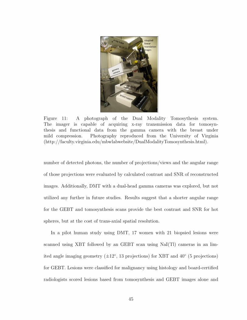
Figure 11: A photograph of the Dual Modality Tomosythesis system.The imager is capable of acquiring x-ray transmission data for tomosyn-thesis and functional data from the gamma camera with the breast undermild compression. Photography reproduced from the University of Virginia(http://faculty.virginia.edu/mbwlabwebsite/DualModalityTomosynthesis.html).

number of detected photons, the number of projections/views and the angular range

of those projections were evaluated by calculated contrast and SNR of reconstructed

images. Additionally, DMT with a dual-head gamma cameras was explored, but not

utilized any further in future studies. Results suggest that a shorter angular range

for the GEBT and tomosynthesis scans provide the best contrast and SNR for hot

spheres, but at the cost of trans-axial spatial resolution.

In a pilot human study using DMT, 17 women with 21 biopsied lesions were

scanned using XBT followed by an GEBT scan using NaI(Tl) cameras in an lim-

ited angle imaging geometry (±12, 13 projections) for XBT and 40 (5 projections)

for GEBT. Lesions were classified for malignancy using histology and board-certified

radiologists scored lesions based from tomosynthesis and GEBT images alone and

45

combined to determined performance metrics. For thresholds listed, x-ray tomosyn-

thesis and GEBT generally had equal sensitivities, but GEBT always provided better

specificity. Results showed that the better specificity provided by GEBT increases

the overall performance of DMT to an accuracy of 95% while better localizing tumors

(Williams et al., 2010).

In an effort to improve upon the quality and quantification of GEBT images

under a limited-angle geometry, an MLEM reconstruction algorithm that utilizes a

priori information was explored. Regularization was applied to object based on XBT

data and attenuation and resolution recovery coefficients were used for projection

operators. Using SIMIND, a Monte Carlo radiation transport simulation package,

projections from a grid pattern of hot spots and a uniform object were generated to

model GEBT scans and reconstructed with and without regularization, attenuation

correction or resolution recovery. Compared to planar projections and previous DMT

studies, accounting for these factors improved quantification of lesion activity and

imaging performance improved with increased angular range, contrast to a previous

DMT study (Gong et al., 2012; More et al., 2007).

The use of DMT has proven to be effective clinically in localizing and identifying

malignant tumors. However, the reconstruction algorithm evaluated in Gong et al.

(2012) as of this writing has yet to be applied to clinically acquired data. In addition,

scatter correction normally accompanies attenuation correction and is noticeable ab-

sence from projection operators. The models and phantoms used in Gong et al. (2012)

46

did not include out-of-view activity, where scattered photons may become more of

a concern for DMT. Nevertheless, DMT may potentially become a valuable clinical

tool for detecting breast cancer.

47

CHAPTER II

GENERAL RADIATION TRANSPORT AND ANALYSIS METHODS

2.1 Monte-Carlo N-Particle Simulator

2.1.1 MCNP5 Overview

The radiation transport code used for the duration of this thesis is Monte Carlo

N-Particle, version five (MCNP5) developed at Los Alamos National Laboratory and

distributed by the Radiation Safety Information Computational Center (RSSIC) at

Oak Ridge National Laboratory (ORNL). The MCNP5 code is capable of neutron,

electron, photon, or simultaneous transport of all three particles through geometries

defined by the user. The strength of this code is the extensive library of point-

wise cross sectional data, which is employed to determine particle interactions. The

MCNP5 code includes all of the physical processes for neutron, electronic, and pho-

tonic interactions, however, only gamma-rays in the low energy regime (< 511 keV)

are simulated in this work. For that reason, neutron and electron dynamics are

not considered. The physical processes included in the MCNP5 code for photons

are photoelectric absorption, incoherent (Compton) and coherent (Thomson) scatter,

and fluorescence. Pair production does not occur in this energy regime and, thus, is

excluded.

The geometry of MCNP is defined in terms of the union, intersection and comple-

48

ments of first and second degree surfaces that bound 3D volumes or cells. The user

defines the physical properties of the cells, including position, elemental composition,

and mass density. The initial conditions for radiative transport, such as the sources

particle type, emission energies, distributions and directions are also defined. Finally,

the user can call a variety of tally types that output information on the particle

dynamics, such as surface flux, and pulse-height spectral measurements. The docu-

mentation that accompanies MCNP5 is extensive, however, the following sections will

outline the basic structure of the MCNP5 input files, which are the cell, surface, and

data cards that define the geometry, source distributions and simulation outputs. It

is recommended that the MCNP5 manual and other primers are consulted for further

details not discussed in this document (Brown et al., 2002; Shultis and Faw, 2011).

2.1.2 MCNP5 Inputs

2.1.2.1 Surface Cards

Surface cards are the building blocks for MCNP simulation geometries. Surfaces

are defined either by functions in Cartesian space [f(x, y, z) = 0] or by a series of

known points that lay on the surface. In this work, defining surfaces functionally

is sufficient to describe all simulation geometries. Table 3 provides a few examples

of simple surfaces cards that have been used in this work. Flat planes, spheres,

cylinders, and other second degree shapes are called using their designated mnemonic

and describing the appropriate coefficients or constants that satisfy the function.

49

Table 3: MCNP5 Surface CardsMnemonic Type Description Equation Card Input

P Plane General Plane Ax+By+Cz−D = 0 ABCDPX Normal to X-axis x−D = 0 DPY Normal to Y-axis y −D = 0 DPZ Normal to Z-axis z −D = 0 DSO Sphere Centered at Origin x2 + y2 + z2−R2 = 0 R

S General Sphere(x−x0)2+(y−y0)2+(z − z0)2 −R2 = 0

x0 y0 z0 R

C/X Cylinder Parallel to X-axis(y−y0)2 +(z−z0)2−R2 = 0

y0 z0 R

C/Y Parallel to Y-axis(x−x0)2+(z−z0)2−R2 = 0

x0 z0 R

C/Z Parallel to Z-axis(x−x0)2+(y−y0)2−R2 = 0

x0 y0 R

CX On the X-axis y2 + z2 −R2 = 0 RCY On the Y-axis x2 + z2 −R2 = 0 RCZ On the Z-axis x2 + y2 −R2 = 0 R

For example, a generalized sphere has the mnemonic, S, and the functional form

(x−x0)2 +(y−y0)2 +(z−z0)2−R2 = 0. To fully describe the generalized sphere, the

coefficients x0, y0, z0, and R are used as inputs. However, a sphere centered at the

origin in Cartesian space would only need R defined, as x0, y0, and z0 are known to

be zero. This has another unique mnemonic, SO. Surfaces have positive and negative

sides, where f(x, y, z) > 0 and f(x, y, z) < 0 are satisfied. For example, considering

a plane normal to the X-axis (PX) at x = 3. For MCNP, the functional form for

this plane is f(x, y, z) = x − 3. Considering the Cartesian point (1, 1, 1), this would

have a negative designation, as 1− 3 = −2. This concept becomes very important in

defining cells in MCNP scripts.

In addition to surfaces, an alternative way to identify cells is with macrobodies, a

50

short hand method for describe 3D regions, comprised of standard surfaces without

explicitly defining each side. This can be accomplished with simple 3D parallelo-

grams, cones, and cylinders. Like standard surfaces, the space within the macrobody

has a negative designation, while all space outside is positive. Taking advantage of

macrobodies when identifying simulation geometries can shorten the MCNP script

and simplify the identification of cells. The following macrobodies described are used

within this work.

RPP: Rectangular Parallelpiped, surfaces normal to major axes

RPP Inputs: Xmin Xmax Y min Y max Zmin Zmax

SPH: Sphere, equivalent to surface equation for general sphere

SPH Inputs: V x V y V z R

where V x V y V z = x, y, z coordinates of center

R = radius

RCC: Right Circular Cylinder

RCC Inputs: V x V y V z Hx Hy Hz R

where V x V y V z = center of base

Hx Hy Hz = cylinder axis vector

R = radius

RHP or HEX: Right Hexagonal Prism

RHP Inputs v1 v2 v3 h1 h2 h3 r1 r2 r3

where v1 v2 v3 = x, y, z coordinates of the bottom of the hex

51

h1 h2 h3 = vector from the bottom to the top

r1 r2 r3 = vector from the axis to the middle of the first facet

The surfaces and macrobodies described here are combined to define and identify the

cell cards. Cell cards are discussed in the next section.

2.1.2.2 Cell Cards

The cell card defines the physical shape, properties, and particle track importance

of an object in the simulation universe. Each cell is uniquely identified by a cell num-

ber, the material or elemental composition, and its mass density. The material can

be substituted for zero to indicate a void cell with no particle track importance, such

as vacuum. Each cell is defined by the surfaces that bound that region. The surfaces

that encapsulate the cell are listed using Boolean logic operators that represent the

unions intersections and complements of surfaces. The union operator (:) is analogous

to the logical OR, while the intersection operator, an empty space ( ), serves as the

Figure 12: An schematic illustrating Boolean Operations in MCNP5. a) The unionof A and B. b) The intersection of A and B

52

logical AND. This is best illustrated with figure 12. The command underneath each

figure describes the highlighted region. The complement operator (#) is analogous

to the logical NOT. Thus the statement #(A B) represents the regions that are not

shared by A and B.

To illustrate how to build cell cards from a set of defined surfaces, a simple example

will be considered. Figure 13 shows two concentric spheres next to a single sphere.

The number inside circles correspond to surface cards and the square numbers are

associated with the cells cards to be built. To start, the surfaces cards for this

geometry are the following.

Figure 13: A simple MCNP geometry consisting of spheres. Circle numbers aresurfaces and square numbers correspond to cells.

15 SO 1.25 $ 1-inch diameter sphere at origin surface

53

16 SO 3.75 $ 3-inch diameter sphere at origin surface

17 S 6.25 0 0 1.25 $ 1-inch diameter sphere along X-axis surface

The identification numbers 15, 16, and 17 are used in the in cell cards to define

the separate 3D regions. Text behind the $ are comments, ignored by MCNP. For

simplicity, the spheres will be void regions with photon importance, but the region

outside the spheres will have no particle importance. The easiest cells to describe are

1 and 3, as these are just the interior of the spheres.

1 0 -15 IMP:P=1 $ 1-inch diameter sphere at origin cell

3 0 -17 IMP:P=1 $ 1-inch diameter sphere along X-axis cell

Recall that the negative in front of the surfaces correspond to inside of the surfaces,

where f(x, y, z) < 0. Cell 2 is simply the union of the outside of surface 15 and the

inside of surface 16.

2 0 15 -16 IMP:P=1 $ 3-inch diameter sphere at origin cell

Finally cell 4, the region outside both spheres, is just the intersection of the outer

sphere surfaces.

4 0 16 : 17 IMP:P=0 $ Outerspace

There are special cell parameter cards that allow for repeated structure capabil-

ity within a simulation geometry. The purpose of these cards is to describe a set

or lattice of cells only once, then define identical structures with slightly different

properties based on the original set. A relevant example of this utilized in this work

is defining the camera collimation, which has several identical septa and bores that

54

would be strenuous to describe individually. The repeated structure capability func-

tions through the Universe Card (U), the Fill Card (FILL) and Lattice Card (LAT).

Cells are given an universe designation with the U card to which those cells belong.

The LAT card can be used to generate a square or hexagonal lattice of cells that can

extend out infinitely within an universe. The FILL card is then used to fill another

cell with the set or lattice of cells within a universe. In the case for collimation, a

septum and bore cell are placed in a universe, which is used to generate a lattice of

septa and bores to fill a rectangular space. These cell parameter cards simplify the

process of generating repeated structures.

2.1.2.3 Data Cards

The data cards include the inputs for the problem type, source definitions, tallies,

materials with element compositions, additional peripheral cards, and the problem

cutoff. One noteworthy peripheral card is the Particle Track Output (PTRAC) card,

which serves as the primary output for these simulations. However, the other data

cards mentioned will be discussed first.

The MODE and PHYS cards are required for specifying which particles are created

and tracked, and what physical processes are needed for the simulation. Both cards

use any permutation of the inputs N, E, and P to signify neutrons, electrons, or

photons particles. The PHYS card has addition inputs for energy and physical process

cutoffs to ignore uninteresting interactions and limit computational burdens. For this

55

work, only photons were required for radiation transport, thus, only MODE:P and

PHYS:P were called for these simulations.

The material specification card (M) is used to define the elemental composition

of cells in the simulation. The inputs for the material card are ZAID values cor-

responding to the atomic number (Z), atomic mass number (A), an identifier (ID),

which is not used in this work, and the atomic fraction or element abundance for that

particular isotope. Another option for specifying materials includes calling neutron

cross sectional libraries, however, these and other cards are not required for gamma

ray transport. The following examples of material cards were used in this work. For

natural water, the ZAID values and material abundances are

M1 1000 2

8000 1

where 1000 and 8000 correspond to hydrogen (Z=1) and oxygen (Z=8) with 1 oxygen

for every 2 hydrogen atoms. A simple material to define is High-Purity Germanium

(Z=32), which is specified as

M2 32000 1.

A more complex material to model is air, which is comprised of a mixture of Carbon

(Z=6), Nitrogen (Z=7), Oxygen, and Argon (Z=18) with atomic fractions of 0.000108,

0.7808, 0.209792, and 0.0093 respectively. Air can be specified in MCNP as

M3 6000 -0.00108

7000 -0.7808

56

8000 -0.209792

18000 -0.0093

where the negative signs denotes atomic fraction instead of element abundances.

The most important and complex data card is the source definition, SDEF. Within

the SDEF card, the user can specify the particles, energies, starting location, emission

direction, and probabilities of emissions in the simulation with source variables. Table

4 shows a condense version of the source variable offered by MCNP5 used in this

work. These variables can be called explicitly as a single value, as an independent

distribution (D), or as a function of another variable distribution. When single values

are not used, but either an independent or dependent distributions are, the source

information (SI), probability (SP), and bias (SB) cards are employed to describe

the distribution. Employing these variables allows for a series of source definitions,

ranging from mono-energetic, isotropic radioactive point sources, or multi-energetic,

collimated volumetric sources.

For this work, the majority of simulated sources are mono-energetic, volumetric,

and isotropic photon emissions, where different cells or objects have different emission

probabilities. Thus, a single energy emission is called using ERG equal to a single

value and the PAR variable is set equal to 2, signifying only photon emission. The

CEL card is used in combination with a distribution number to identify the source

emission probabilities for each cell. The CEL distribution was then used as the

dependent variable to identify the volumetric distribution of the sources. For example,

57

Table 4: MCNP5 Source Variables for the SDEF cardVariable Meaning DefaultCEL cell Determined from Location

and possibly directionERG Energy (in MeV) 14 MeVDIR µ, the cosine of the angles

between VEC and the direc-tion of the source emission

µ is sampled isotropically

VEC Refercen vector for DIR Require unless isotropicemission

POS Reference point for positionsampling, normally center ofobjection

The origin: 0,0,0

RAD Radial distance of the posi-tion from POS to AXS

0

EXT Distance from POS alongAXS

0

AXS Reference vector for EXTand RAD

No direction

X X-coordinate of position No XY Y-coordinate of position No YZ Z-coordinate of position No ZPAR Particle type 1 = neutrons

2 = photons3 = electrons

a box object, like the torso, has its source distribution uniformly defined using the

X, Y, and Z source variables and providing the x-, y-, and z-range for the torso. For

a spherical object, like a tumor or lesion, the POS and RAD variables are called

to identify a sphere’s central position and radius vector, from zero to the radius

magnitude. These variables are called with FCEL, or as a function of the CEL

distribution, such that the source probability within the torso and tumor depend

upon the appropriate volume. In short, the spatial distribution of emission within a

58

cell is defined to be uniform, but its probability of emission is dependent upon the

cell.

Tally cards are called to specify output information from simulations. There are

numerous tallies that are useful for various applications, but related to this work, two

specific tallies are pertinent. The F2 tally calculates the flux average over a surface in

units of particles per centimeter squared. Employing this tally on the front and back

surfaces of a detector can offer insight on the count efficiency of the detector. The F8

tally generates a pulse height distribution of energy deposited into a detector. Two

cards that should be used in combination with the F8 tally are the energy binning

card (E), for sorting out irrelevant low energy interactions and appropriately binning

relevant energy domains, and the Gaussian energy broadening card (FT), to provide

an energy-dependent energy resolution to the pulse height tally. These tallies and

support cards can provide complementary information to the output and analysis of

the PTRAC card.

The final cards required for the MCNP script are the history cutoff (NPS) and

the random number generation card (RAND) cards. The NPS limits the number of

particles to run for the simulation, such that NPS 5000 would end the simulation

after 5000 generated particles. RAND specifies the random number generator used

to initialize the simulations. The GEN keyword uses a type of pseudorandom number

generator, while conversely, the SEED keyword can be used to specify a seed number

to repeat initial conditions.

59

2.1.3 Particle Track Output Card

The Particle Track Output (PTRAC) card is a peripheral card that generates an

ASCII or binary file that lists the entire interaction history for user-filtered events.

PTRAC offers a wealth of information about particle histories that cannot be known

in realistic radiation detection and measurement task. For every collision in a particle

history, the Cartesian position, cell number, material, direction, energy, collision type

and time of interaction for the particle is listed. Without any keyword filters placed

on the PTRAC card, every particle’s event history would be saved, resulting in an

extremely large file with irrelevant information. PTRAC files can be limited by

output control keywords such as MAX, which sets the maximum number of written

event histories, or WRITE, which controls whether all event information or only

position and cell numbers are written to the PTRAC output file. In addition to

output control keywords, event and history filters can be placed on the PTRAC card

to only store relevant events. In particular to this work, only events that deposit

energy in the radiation detector are written to a file. To facilitate event filtering,

the EVENT, TYPE, and TALLY filters are utilized to save necessary information

for pulse-height spectra and image generation. The EVENT keyword specified that

the source emission, collisions, and terminating history are written to the output file.

The TYPE keyword specified that only photons are saved, and the TALLY keyword

ensured that any event that contributed to the pulse height tally on the detector

would write the entire event history to the PTRAC file.

60

The format of the PTRAC output file is nontrivial, but necessary to understand

and extract the pertinent information for an event. Given the filters placed on the

PTRAC card, the output file has the following format for each event.

Particle header: [Particle Number Source Flag (1000) Triggered Filter]

Source header: [Collision flag (4000 or 5000) Node Number Source Type Cell

Number Material Number Number of Collisions]

Source information: [Position Coordinates Direction Vector Energy Weight

Time]

1st collision header: [Collision flag (4000 or 5000) Node Number Cross Section

Info Collision Type Cell Number Material Number Number of Collisions]

1st collision information: [Same format as source information]

...

nth collision header: [Collision flag (5000) Node Number Cross Section Info Col-

lision Type Cell Number Material Number Number of Collisions]

nth collison information: [Same format as source information]

final header: [Collision flag (9000) Node Number Termination Type Branch Num-

ber Cell Number Material Number Number of Collisions]

nth collision information: [Same format as source information]

The particle header consists of the particle number, the source emission flag (1000),

61

and the filter which cause the event to be written to file, in this work, the pulse

height tally. The source header, and most other collision headers, consists of either

the collision flag (4000) or particle termination flag (5000), the type of collision, the

cell and material the photon originated and a single value indicating the number

of collisions in the event thus far. Source and collision information consists of the

Cartesian coordinates or position of the collision, the direction the particle travels,

the energy of the particle, and a time since the beginning of the current event. The

nth collision header and final header have some redundant information, however,

the final header has the final event flag (9000) to indicate that there are no more

events listed in the particle history. After the final head and collision information,

the PTRAC output file would continue with the next particle history, repeating the

PTRAC format.

There is a wealth of information within MCNP5 tallies and the PTRAC that is

not related to parsing the output file for generating images, including cross sectional

library calls, flags for indicating interaction nodes, particle weights, and even timing

information. However, the position, energy, and types of events listed in each particle

history is important and required for generating energy spectra and images. Reducing

the PTRAC output to imaging data requires an understanding of the PTRAC format,

its included information and a method for parsing through all the particle histories.

In the next section, the method and scripts for parsing the PTRAC output from

MCNP5 will be discussed.

62

2.2 MATLAB PTRAC Parser

The program MATLAB (short for MATrix LABoratory) (The MathWorks, Inc,

Natick, MA) was employed for much of the data analysis in this work. Its built-in

functionality makes MATLAB a versatile tool for a range of applications, including

reading ASCII files, image processing, and analysis. The MATLAB script for pars-

ing through MCNP5 PTRAC output files has been adopted from code used by Dr.

Benjamin McDonald. A generalized method for parsing the PTRAC output file for

energy deposited into the detector is described.

1. Open the file for line by line reading. Skip through the PTRAC header and

locate the first particle history by searching for the source header flag, 1000. Initialize

a while loop that tests for the end of the file.

2. Scan/Read the source header line and save as a variable. Initialize another while

loop that will test for the end of the particle history. This can be the next source

header flag, 1000, or the final event header 9000. Setup an alternating scan/read line

commands that reads and saves the collision headers and collision information. This

should end with the termination header and collision information that follows.

3. Determine the energy deposition: For every collision event, first determine if the

interaction occurred in the detector cell. If so, then in general, the energy deposition

for the event is the difference between the particle energy before and after the collision.

If the interaction process is a fluorescence event, then the energy deposition is zero for

the event. If the collision flag has a value of 5000, then the energy deposition is the

63

energy for that event. Any event that follows a 5000 flag that is not accompanied by

a final event flag indicates a re-emission, and thus, energy deposition is the negative

of the event energy. After parsing the particle history, sum the energy deposition

from each event for the total energy deposited.

Once the energy deposition is determined, energy blurring can be applied to sim-

ulate energy resolution and that final energy can be binned to generate the total

pulse-height spectrum. The information within the particle history can also be used

to determine other properties of the particle track, including the type and number

of interactions (photoelectric, incoherent and coherent scatter), x-ray fluorescence

events from shielding, and interaction locations within the detector. Once the loca-

tion of flags for user-defined cells and interactions processes within a particle event

are known, it is trivial to extract that information for use. The relevant properties

of the particle histories for imaging that are scored for this work are discussed in the

next section.

2.3 Imaging Metrics and Analysis

2.3.1 Pulse Height Spectrum

The total pulse height spectrum can be generated from binning the individual

energy depositions for each particle history. Knowing the entirety of the particle

track and its interactions enables us to categorize details about energy spectra that are

normally occult from experimentally-acquired spectra. Within the NBI simulations,

64

we can investigate the nature of scatter contributions and image contamination from

out-of-view sources. Scattered photons that contribute to images have lost their origin

information, becoming a source of noise which could degrade image quality. Scatter

order, or the number of Compton scatters outside the detector, is determined by

totaling the number of incoherent interaction flags (-1) when the cell number is not

equal to the detector cell number. The photon origin is indicated by the cell number

within the source information line of the particle history. With this information on

scatter order and photon origin, specific pulse height spectra can be plotted along

with the total pulse-height spectra. Given an energy discrimination cutoff, or energy

window, around the primary photopeak, scatter and torso fraction can be determined

as the fraction of scattered and torso counts compared to the total number of counts

within the energy window. Lower scatter and torso fraction are desired, as this

signifies more accurate projections and less out-of-view contamination of collected

images.

2.3.2 Image Formation

The main purpose of detecting and collecting photons is the formation of an image

that describes the anatomic and functional differences within a subject. An energy

window is set for events to contribute to images. For events that satisfy the energy

cutoff criterion, the position of the first particle collision within the detector is taken

as the event location. Spatial blurring of the Cartesian coordinates, representing

65

the spatial resolution of the detector, may be applied to simulate detector response

or could be omitted for a detector system with perfect spatial resolution. The new

coordinates of the events are binned to generate an image. For visual display, a

3×3 mean filter is convolved with projection images to highlight prominent features,

however, any imaging-metric calculations are performed on initial, unfiltered images.

The method for visualizing the size and intensity of image features is accomplished

by drawing line profiles through those objects. Line profiles provide a sense of relative

intensity between tumor signal compare to the background of the images, as well as

image noise. In essence, line profiles provide a qualitative assessment of the object

contrast and SNR. Quantitative measures of tumor contrast and SNR can be found

by drawing ROIs (Region of Interest) around areas of background and hot spots

and calculating their average intensity. The following equations are applied to those

averages to determine image contrast and SNR.

Tumor Contrast =Mean Tumor Signal −Mean Background

Mean Background(3)

Tumor SNR =Mean Tumor Signal −Mean Background

STD Background(4)

In general, higher contrast values correspond to detectable variations, which may

be indicative of anatomical or functional changes in the subject. For SNR, the Rose

criterion dictates that tumor SNR values of approximately 5 have a 100% detectability

rate, while SNR values < 5 have a lower chance of detectability (Bushberg and Boone,

66

2002; Cherry et al., 2012).

2.4 Chapter Summary

This chapter describes the generalized simulations methods utilized in this body of

work. The MCNP5 simulation package was described, covering the basic components

for building and evaluating simple imaging geometries. The PTRAC card and output

file are described, which enables the user to save a list of particle histories that satisfy

certain conditions of interests. MATLAB is used for parsing the PTRAC output and

performing analysis upon generated pulse height spectra and images. The energy

spectra are broken down into scatter order and photon origin to determine the source

and magnitude of scatter and artifacts. The methods for generating and analyzing

images with line profiles and image contrast and SNR is also described. These meth-

ods and metrics are utilized for all projection imaging tasks. Other methods specific

to a particular task are described in their chapter in which the method is applied or

employed.

67

CHAPTER III

GERMANIUM DETECTOR CHARACTERIZATION

3.1 Introduction

For the last several years, our research group has collaborated with Pulse Height

Detectors Company (PHDs Co.) (Knoxville, Tennessee) in their efforts to fabricate

position-sensitive Germanium cameras for various applications. A large part of this

collaborative work involves rigorous detector and camera characterization of their sys-

tems. Figure 14 shows a timeline of the HPGe systems PHDs Co. has developed in

recent years. The earliest HPGe systems had attached LN2 dewars, making it imprac-

tical for some imaging applications. Later systems substituted the heavy dewars for a

mechanical cooler, reducing the weight of the detector and making it more compact.

The MI4-series shifted the detector to the front and moved the electronics behind

for an improved imaging geometry, but exposed wires, components and an outlying

power controller made for a less than aesthetic system. The most recent HPGe detec-

tors, the GGC-series, are general-purposed systems, entirely packaged and compactly

sealed with mobile capabilities and integrated mounts for pinhole or parallel-hole

collimation. These advancements have propelled these traditional spectrometers to

commercially viable imaging systems.

In previous studies, our group has characterized the performance of different HPGe

68

Figure 14: A timeline illustrating the HPGe systems fabricated and developed byPHDs Co. Within this time period, HPGe systems have progressed from requiringheavy LN2 dewars attached, to compactly packaged, mobile systems.

detectors, including the NP-, MI4-, and GGC-series (Johnson et al., 2011a,b, 2012;

Campbell et al., 2013). In this chapter, the characterization methods for the MI4.2

and GGC1.1 detectors are discussed, hereafter refer to as MI4 and GGC unless spec-

ified. At the time of characterization, the objectives differed between the two de-

tectors, resulting in slight variations in performed methods between the MI4 and

GGC in this document. The primary goal for characterization of the GGC was to

demonstrate its imaging capability, while measurements on the MI4 are used in the

development of an HPGe detector model for breast imaging (Chapter IV). Despite

this, the intrinsic properties of the HPGe detectors are measured closely, but not

strictly adhering, to the NEMA NU 1-2007 standards for gamma cameras, as these

69

standards are designed for monolithic systems (scintillators) as opposed to segmented

detectors (NEMA, 2007). The intrinsic properties investigated for the MI4 and GGC

are detector efficiency, spatial resolution, energy resolution, and flood field uniformity.

In addition, the planar imaging capabilities of the GGC and MI4 are explored using

line sources and hot spheres phantoms.

3.2 Materials and Methods

3.2.1 System Specifications

Displayed in figure 15 and 16 are the MI4 and GGC imaging systems. Even with

the differences in packaging, both systems have an equivalent underlying architec-

ture. The MI4 and GGC are cylindrical double-sided strip detectors (DSSD) with

physical dimensions of 90-mm diameter and 10-mm thick. The germanium detectors

are designed with a set of 16 × 16 orthogonal strips of 4.75-mm width and 5-mm

pitch with 0.25-mm gaps between strips. These strip dimensions yield an active area

of 55.1 cm2. The systems have a forward-facing detector, with a mechanical cryostat

capable of cooling down to 60 K, and FPGA-based readout electronics placed behind.

For the MI4, a power controller box monitors all system properties, including tem-

perature and HV bias, while digitized signals are read out through a single USB-2.0

port to the custom software, Imager32, packaged with all PHDs Co. systems. For the

GGC, all data acquisition, system control, and system monitoring functions are ac-

cessed through Imager32 and the USB-2.0 port, without a separate power controller.

70

Figure 15: Photographs of the MI4 system from multiple vantage points. The com-ponents of the system are labeled, from the mechanical cooler on top, to the entrancewindow and readout electronics. The parallel-hole collimator lend to our group byDilon Diagnostic can be seen in the side view photo.

An integrated assembly allows for interchangeable mounting of parallel-hole and pin-

hole collimators, whose designs were based on simulations for optimizing parallel-hole

(Chapter V) and single pinhole collimation for small-animal imaging (Johnson et al.,

2011b; Campbell and Peterson, 2011).

As described in chapter I, pulse signal analysis is applied to all events to achieve

position interpolation finer than the strip width and detector thickness. Using the

50% CFD time difference on opposite side collection strips, events are sorted into

1-mm depths bins. In addition, the difference in the magnitude of transient signals

71

Figure 16: Images of the GGC system from multiple angles. Brackets attached tothe entrance window allows for the mounting of parallel-hole collimation or a pinholeaperture. The system is completely self-contained with the mechanical cryostat, lite-readout, and a handle for mobile capability.

induced upon neighboring strips are used to estimate lateral position into nine 530-µm

bins.

3.2.2 Intrinsic Detector Measurements

3.2.2.1 Detector Efficiency

Efficiency measurements were performed for the MI4 and GGC systems. For the

MI4, a 57Co flood source with an activity of 0.60 MBq was centered and aligned at

a 50-cm distance from the detector and imaged for 12 hours to ensure good counting

statistics. For the GGC, a 0.22-MBq 57Co source was placed 56 cm away from the

detector and imaged for over 24 hours for good statistical quality. An energy window

72

of ±3 keV around the 122-keV photopeak was used to determine the number of

total counts (N). Equations (5) and (6) were used to calculate the intrinsic detector

efficiency (ε):

ε =N

S

4π

Ω, (5)

Ω =Area

d2, (6)

where S is the number of emitted photons, calculated from the known acquisition

time, the branching ratio of 122 keV for 57Co, and its radioactivity, Ω is the solid

angle between the point source and detector area, and d is the distance between the

source and detector.

3.2.2.2 Energy Resolution

The flood scan performed with the MI4 for intrinsic detector efficiency was also

used for determining its energy resolution. Conversely, a flood illumination with mul-

tiple radinuclides was performed to measure and demonstrate the energy resolution

of the GGC. Approximately 37 MBq of 57Co & 99mTc, and 20 MBq of 123I were placed

350 cm from the GGC and imaged for 30 minutes. An pulse-height spectrum was

generated from the scan and the FWHM of the 122, 136, 140, and 159 keV photopeaks

were measured.

73

3.2.2.3 Intrinsic Spatial Resolution

The intrinsic spatial resolutions of the MI4 and GGC were measured using the

Edge Spread Function (ESF) method, similar to acquiring a pre-sampled Modulation

Transfer Function in autoradiography (Giger et al., 1986). Using a tungsten block,

half of the detector entrance was shielded at a known angle through the center of its

FOV. A 57Co flood source was placed 60 cm away from the detector and counts were

acquired for 24 hours. Line profiles orthogonal to the edge response were shifted and

plotted appropriately to visualize the ESF. A logistic function was fitted to the ESF

and differentiated to generate a Line Spread Function (LSF). The LSF was modeled by

a Gaussian function, whose FWHM was measured for the intrinsic spatial resolution.

This process was completed for both the x- and y- dimensions.

3.2.2.4 Flood Field Uniformity

The flood field uniformity was measured in the useful and the central FOV for the

MI4 and GGC in accordance with NEMA protocols. According to NEMA standards,

acquired images require a count density > 10,000 counts per cross strip.The UFOV

included all collection strips with two neighboring strips, which eliminated the four

bordering strips of the FOV. The CFOV was defined as 75% of the UFOV, which

corresponds to removing an additional set of strips along the edge of the UFOV. Two

3-hour flood scans were performed using a 37-MBq 57Co source. The first flood scan

was conducted without any corrections to the data. This scan was used to generate

74

normalization factors to correct for non-uniformities in the entire FOV. The second

flood scan then applied these corrections. The integral uniformity was calculated for

both flood scans in the UFOV and CFOV using equations (7):

Integral Uniformity =max−minmax+min

× 100%. (7)

where min and max are the minimum and maximum pixel intensities of the image.

The differential uniformities in the x- and y-dimensions are determined by the maxi-

mum, or worst, uniformity measurements between 5 consecutive pixels in a single row

or column.

3.2.3 Camera Measurements

The parallel-hole collimator and the pinhole aperture were mounted on the de-

tector systems to demonstrate their imaging performance. A lead low energy high

resolution (LEHR) parallel-hole collimator, loaned to us by Dilon Diagnostics (New-

port News, VA, USA), was placed in front of the MI4. This collimator has 1.85 mm

hexagonal-shaped holes with 20-mm length and 0.3-mm thick septa thickness. The

parallel-hole collimator packaged with the GGC has 1.5-mm wide hexagonal-shaped

holes with 0.2-mm septa and 20-mm overall thickness. The single-lead pinhole aper-

ture for the GGC has a 1-mm diameter aperture with a 60 degree opening angle and

a focal length of 8 cm. Experiments performed with these collimators were executed

based on procedures for gamma cameras outlined in the NEMA standards.

75

The spatial response of the MI4 and GGC was measured with their parallel-hole

collimators attached. Capillary tubes with a 1-mm inner-diameter were filled with

a 99mTc solution and scanned at a distance of 6.0 cm away from the MI4 and 6.7

cm away from the GGC. Projections of these line sources were acquired until more

than 103 counts were collected in the hottest-intensity pixels. LSFs were generated

and fitted to Gaussian functions from a single line source projections by summing

orthogonally across three collecting strips. The spatial response of the camera was

taken as the average of the FWHM and FWTM of the Gaussian fits. Measurements

were made for both the x- and y-dimensions. Comparisons to the expected spatial

response were made using analytic formulations for geometric (8) and total system

resolution (9) given the measured intrinsic spatial resolution Ri (Anger, 1967):

Rg =d(le + x+ c)

le(8)

R =√R2g +R2

i . (9)

Here, d is the collimator-hole diameter, le is the effective collimator length adjusted

for attenuation, x is the source-to-collimator distance, and c is the spacing between

the bottom of the collimator and the detector material, assumed to be 14.6 mm.

Analytic FWTM was assumed to be 1.83 times the recorded FWHM.

One feature of these position-sensitive HPGe detectors worth highlighting is its

Depth-Of-Interaction (DOI) capability. To demonstrate this attribute, projections of

76

Figure 17: A photograph of the breast phantom. The 10 cm × 10 cm × 6-cm thickplastic box was designed to cover the HPGe camera FOV and mimic an average-sizedbreast under mild compression. The 1 mL (1.2-cm diameter) and 0.25 mL (0.8-cmdiameter) spheres are suspended inside.

two capillaries on and off-axis of the pinhole collimator were acquired with the GGC.

A schematic diagram of the experiment appears in figure 25a. The on-axis capillary

was placed at a distance of 6.7 cm away from pinhole, while the second was positioned

3.0 cm (25) off-axis of the pinhole. Projections of these line sources were acquired

until more than 103 counts were collected in the hottest-intensity pixels. The line

source projections were visualized as both an x, y image as well as lateral position

versus depth images to demonstrate the DOI estimation capability.

One potential biomedical imaging application for HPGe DSSDs is diagnostic

breast imaging. A breast phantom was developed in our lab for modeling planar

breast imaging scans with the HPGe cameras (figure 17). The phantom consisted of

a plastic box with dimensions of 10 cm × 10 cm × 6-cm thick and a holder to position

the plastic spheres anywhere within the volume. In this experiment, two spheres with

77

Figure 18: A projection image of the 57Co flood sources acquired with a) the MI4and b) the GGC. The cylindrical HPGe detectors exhibit an 8-cm in diameter FOV.The black lines correspond to gaps between the strips. These acquisitions employedan energy window of ±3 keV around 122 keV and was used to calculate detectorefficiency.

volumes of 1 mL and 0.25 mL were placed in the phantom at a depth of 1 cm from the

parallel-hole collimator with 99mTc activities of 5.9 MBq and 1.3 MBq, respectively.

The phantom was imaged with three backgrounds: One with an air background, one

with non-radioactive water as a scattering medium, and one with a 488-MBq back-

ground of 99mTc, modeling a tumor to background ratio of approximately 5:1. Each

projection image was acquired for one minute with an energy window of ±2 keV at

140 keV with both the MI4 and GGC. Contrast and SNR values were determined by

first drawing a 9×9 signal ROI centered on the hot spheres and a 27×27 background

ROI adjacent to the hot sphere. Equations (3) and (4) were applied to the ROIs to

calculate contrast and SNR.

78

3.3 Experimental Results

3.3.1 Intrinsic Detector Measurements

The projections for calculating the intrinsic detector efficiency of the two detec-

tors are displayed in figure 18. The intrinsic detector efficiencies of the MI4 and GGC

were measured to be ∼53% at 122 keV. These efficiency measurements are compa-

rable to previously characterized HPGe detectors (Johnson et al., 2011a,b). Current

pulse processing of events in these HPGe detectors only includes photons with com-

plete deposition of charge within one cross-strip. This also includes events that may

Compton scatter followed by photoelectric absorption within a cross-strip, but would

exclude any events where charge collection is shared among neighboring strips on

either detector side.

The pulse-height spectrum for the MI4 is displayed in figure 19 and the multiple

radionuclide spectrum with the GGC is displayed in figure 20. With the MI4 detector,

the two photopeaks of 57Co are clearly distinguishable, a feature normally occult

in detectors with poorer energy resolution. For the 122 keV photopeak, a FWHM

of 1.02% is measured. With the multi-radionuclide scan from the GGC, the main

photopeaks of 57Co, 99mTc and 123I are clearly visible. In addition, the Kα and

Kβ characteristic x-ray peaks of lead are also distinguishable. The measured energy

resolutions of the 122, 136, 140, and 159 keV photopeaks are 1.28%, 1.01%, 1.11%

and 1.02%, respectively. The GGC capability to resolve the 136 keV secondary peak

of 57Co and the main 99mTc peak at 140 keV clearly demonstrates the excellent energy

79

Figure 19: The pulse-heigth spectrum resulting from the flood scan of 57Co with MI4.The excellent energy resolution of HPGe allows for distinguishable Kα and Kβ leadcharacteristic x-ray peaks, as well as separation between the 122 keV and 140 keVphotopeaks, usually indistinguishable with other detectors.

resolution of the system.

Representative results of the intrinsic spatial resolution acquired using the ESF

method are displayed in figure 21 and 22, including the logistic fit to the ESF data

and the Gaussian fit to the LSF data. The FWHMs of the LSFs were measured to be

1.9 mm and 1.5 mm in the x- and y- dimensions for the MI4, respectively, while the

intrinsic resolution of the GGC was 2.5 mm and 2.6 mm for the x- and y-dimensions,

respectively.

Representative projections for measuring the flood field uniformity of the MI4 and

GGC are displayed in figure 23. The calculated uniformities in the UFOV and CFOV

for the uncorrected and corrected projections for both detectors are shown in Table

80

Figure 20: The energy spectrum resulting from the flood scan with multiple ra-dionuclides. Photopeaks are identified and labeled with FWHM measurements. Theexcellent energy resolution of HPGe allows for distinguishable Kα and Kβ lead char-acteristic x-ray peaks, as well as separation between the 136 keV and 140 keV pho-topeaks.

Table 5: MI4 Flood Field Uniformity MeasurementsStandard Flood Corrected FloodUFOV CFOV UFOV CFOV

Integral 45.90% 45.90% 5.57% 5.57%Differential Row 29.91% 29.91% 4.13% 4.13%

Differential Column 32.54% 32.54% 3.76% 3.76%

Table 6: GGC Flood Field Uniformity MeasurementsStandard Flood Corrected FloodUFOV CFOV UFOV CFOV

Integral 22.19% 17.90% 6.12% 6.08%Differential Row 15.54% 14.75% 4.38% 4.38%

Differential Column 14.69% 14.14% 4.86% 4.79%

81

Figure 21: a) A projection image of the partially covered MI4 detector system. Thedashed-line box represents the horizontal line profiles that comprised the ESF. b)The ESF dataset and its Logistic fit. c) The LSF was derived by differentiating theLogistic function. The spatial resolution was taken as the FWHM of the LSF.

82

Figure 22: a) A projection image of the partially covered GGC detector system. Thedashed-line box represents the horizontal line profiles that comprised the ESF. b) TheESF dataset and its Logistic fit. The LSF was derived by differentiating the Logisticfunction. The spatial resolution was taken as the FWHM of the LSF.

83

Figure 23: Processed images of the UFOV for determining flood field uniformity.Uncorrected and corrected images of the UFOV from a) the MI4 and b) the GGC.Normalization factors generated using the uncorrected image were applied to correctthe subsequent flood. The solid black line outlines the CFOV within each image.

5 and 6. With applied corrections to the CFOV, integral uniformities are between

5-6% for both detectors. However, the differential uniformities for MI4 and GGC

are around 4.2% in the x-direction, but an uniformity difference in the y-direction of

3.76% and 4.8% for MI4 and GGC, respectively, is observed.

3.3.2 Camera Measurements

The spatial response of the detectors with the parallel-hole collimator are illus-

trated in figure 24 and FWHM and FWTM measurements are listed in Table 7 and 8.

84

Figure 24: Projection images of capillary tubes and line spread functions demon-strating the spatial response of a,b) the MI4 and c,d) the GGC. The dashed-line boxcontained the vertical line profiles summed together to form a single LSF, which is fit-ted to an Gaussian function. The average FWHM and FWTM of the LSfs were takenfor the MI4 and GGC spatial response at a depth of 6.0 and 6.7 cm, respectively.

Both detector systems exhibit a slight asymmetry in their spatial response reflected

in their different spatial resolutions. Comparing the measured spatial response to

the theoretical object resolution, we observe similar values for the response in the x-

dimension for both detectors. However, measurements for the y-dimension exhibit less

agreement with theoretical predictions, with the largest difference with the FWTM

of the MI4.

The results for demonstrating the DOI capability of the GGC are displayed in

figure 25b and 25c. The black lines in the depth projections represent to the gaps

between the collection strips. With 1-mm depth binning, we observed an angular

85

Table 7: MI4 Spatial Response at 6.0 cm from the Parallel-Hole CollimatorX-Resolution (mm) Y-Resolution (mm)FWHM FWTM FWHM FWTM

Measured 9.11 16.60 9.80 17.85Expected 9.23 16.90 9.16 16.75

Table 8: GGC Spatial Response at 6.7 cm from the Parallel-Hole CollimatorX-Resolution (mm) Y-Resolution (mm)FWHM FWTM FWHM FWTM

Measured 8.31 15.15 7.84 15.50Expected 8.29 15.17 8.09 14.80

intensity profile from the line source placed off-axis of the pinhole. Without DOI

estimation, this angular projection would appear as a blurred column of response,

similar to the on-axis projection, but extended laterally.

Projections of the breast phantom with various backgrounds are displayed in figure

26 and contrast and SNR values are listed in table 9. Comparing the images of

the spheres suspended in air and water, there was little to no degradation in their

overall shape and size observed. When imaging the hot spheres with a warm 99mTc

background, both the 1.2-cm and 0.8-cm diameter spheres were detectable above the

background. Considering the Rose criterion for SNR, the 1 mL sphere would have a

100% chance to be detected, while the 0.25 mL is still visible even with a SNR < 5.0.

Slight differences in contrast and SNR can be attributed to the different collimators

attached to the MI4 and GGC.

86

Figure 25: a) A schematic diagram of the DOI demonstration. Two 99mTc-filledcapillary tubes were imaged with different lines of sight, on and off-axis of the pinholeaperture. b) The x,y projection of the two capillaries integrated over all 10 depths. c)The lateral position versus depth profiles of the two capillaries. The off-axis capillaryprojection exhibits a response at the same angle as the offset capillary. WithoutDOI estimation, the off-axis capillary would appear as an enlarged, blurred columnof response.

Table 9: Contrast and SNR values for hot spheres in images of the breast phantom1.0 mL sphere 0.25 mL sphere

Contrast SNR Contrast SNRMI4 1.29 5.61 0.36 1.52GGC 1.26 7.21 0.42 2.41

87

Figure 26: Projection images of the breast phantom containing 1 mL and 0.25 mL hotspheres at a depth of 1 cm from the collimator acquired with the MI4 and GGC. MI4images with spheres a) suspended in air, b) suspended in a water scattering mediumand c) with a 488-MBq 99mTc background. GGC images with spheres d) suspendedin air, e) suspended in water and f) with a hot background. Very little degradationin the spatial response is observed in the presence of a water scatter medium. Witha tumor to background ratio of 5:1, both hot spots are visible above background.

88

3.4 Discussion

The fabrication of the MI4-series of detectors signified the first steps in designing

an imaging system with an optimal geometry. However, the GGC is the first version of

a compactly packaged HPGe detector integrated with collimators for general-purpose

use. This study strove to characterize and evaluate the intrinsic properties and imag-

ing capabilities of these systems. One of the premier features of HPGe detectors is

its excellent energy resolution. With ∼1% FWHM at relevant energies for biomedical

imaging, HPGe detectors are able to resolve photopeaks separated by only a few keV.

This property of HPGe detectors enables multi-isotope SPECT imaging with 99mTc-

and 123I-labeled radiotracers, as well as superb scatter rejection capability; demon-

strated when no degradation of object size or shape was observed when imaging the

breast phantom. The energy resolution allows for tight energy windows (±2 keV

at 140 keV) to be utilized so that low-angle scattered photons do not contribute to

acquired images.

Furthermore, HPGe detectors exhibit favorable features for single-photon imag-

ing. Using the integrated parallel-hole collimator, the MI4 and GGC were capable

of defining sub-centimeter sized spheres in a 5:1 tumor to background environment

at a 1-cm depth. This finding shows the potential for use of these systems in a

clinical setting. The DOI capability of the GGC may offer additional benefits for

SPECT imaging by enhancing parallax recovery and improving the image quality of

reconstructed images.

89

Even with its current performance, improvements can still be made to the HPGe

detectors. The MI4 had a measured intrinsic spatial resolutions less than 2 mm in

both x and y dimensions, while the GGC system currently exhibit 2.5 mm resolution.

Additionally, current event analysis excludes photons that deposit energy across two

collecting strips on either the cathode or anode side of the detector, which reduces

efficiency. Work towards employing more sophisticated pulse processing for resolving

gap and Compton scattering events is underway. Also, exploring other compact

packaging configurations may offer further improvements in GGC performance.

A constant challenge of the HPGe DSSDs are the gap regions in between collection

strips. Given the current pulse processing utilized with these systems, events that

occur within the gaps regions are not processed, negatively impacting count efficiency.

In addition, the effect of the gaps extend to the pixels along the edges of strips,

which further reduces count efficiency. This is the major cause of non-uniformity

in uncorrected projections, evident with uniformity values upwards of 46% and 25%

with MI4 and GGC, respectively. Even in the corrected projections, Poisson statistics

can only contribute to errors between 3% and 1.5%, as the mean number of counts in

these images is between 1,000 and 5,000 counts per pixel. The remaining error could

be attributed to the effects of the gaps, which are still observable in projections even

after normalization factors are applied. It is expected that adopting inter-detector

scattering event processing would improve system efficiency and uniformity while

reducing the effects of the gap regions.

90

Figure 27: A photograph of the GGC1 detector crystal (left) and the new GGC2detector crystal (right). The 14-cm diameter crystal of the GGC2 has the largestFOV of any HPGe DSSD to date.

In addition to our efforts of improving current HPGe DSSD performance, construc-

tion on the next iteration of compact HPGe DSSDs has been completed. Displayed in

figure 14 is the GGC2 detector as well as the GGC1 and GGC2 crystals in figure 27.

The GGC2 has a 14-cm diameter FOV, with 7.75-mm strips and gaps of 125 microns,

half the size of previous HPGe detectors. The GGC2 is the largest position-sensitive

HPGe detector fabricated to date. With an increase in the crystal size and a reduc-

tion of the gap width, the larger FOV of the GGC2 may afford increases in absolute

count sensitivity, which could improve SNR measurements in pre-clinical and clinical

biomedical imaging applications.

3.5 Chapter Summary

In this chapter, the intrinsic properties of the MI4 and GGC HPGe detectors

were characterized. Energy resolutions of ∼1% at energies between 122-159 keV were

91

observed in pulse-height spectra. Flood scans registering only single cross-strip events

revealed a detector efficiency of 53% and a corrected uniformity of ∼5% at 122 keV for

both detectors. Finally, spatial resolutions of ∼1.5 mm and ∼2.5 mm were measured

using the Edge Spread Function method for the MI4 and GGC, respectively. The

imaging capabilities were demonstrated with a LEHR parallel-hole collimator with

the MI4 and integraed parallel-hole and pinhole collimators packaged with the GGC.

Camera spatial response for the GGC was approximately 8 mm for a 1-mm diameter

line source at a distance of 6.7 cm away from the collimator and depth estimation

with 1-mm bins was sufficient to differentiate oblique sources and demonstrate DOI

capability. In addition, sub-centimeter hot spheres were detectable in a 5:1 tumor

to background environment with both imaging systems. In chapter IV, the intrinsic

properties of the MI4 detector will be applied to the development of a HPGe breast

imaging model.

92

CHAPTER IV

INVESTIGATING POTENTIAL BENEFITS OF GERMANIUM CAMERAS FORBREAST IMAGING

4.1 Introduction

Mammography has long been the standard technique for the screening and detec-

tion of breast cancer. However, mammography performance deteriorates when imag-

ing denser breast tissue (Rosenberg et al., 1998). Nuclear Breast Imaging (NBI), also

referred to as Scintimammography, Molecular Breast Imaging (MBI) and Breast Spe-

cific Gamma Imaging (BSGI), is a technique that utilizes specifically designed gamma

cameras to image the distribution of 99mTc-sestamibi, which exhibits higher uptake

in malignant tissues than healthy tissue (Delmon-Moingeon et al., 1990). These

techniques have less dependence on tissue density and higher sensitivity than mam-

mography for the detection of sub-centimeter diameter tumors (Garibaldi et al., 2006;

Tornai et al., 2004; Mueller et al., 2003; Robert et al., 2011; Judy et al., 2010).

One benefit of using semiconductor detectors for NBI is that their superior energy

resolution (ER), compared to scintillators, allows for better separation of scattered

photons from primary counts. Cadmium Zinc Telluride (CZT) is a room temperature

semiconductor, typically pixilated into millimeter-scale elements, that has seen use in

biomedical imaging (Mueller et al., 2003; Robert et al., 2011). Utilizing small pixel

0The work in this chapter has been published in the IOP journal, Physics in Medicine and Biology.The text of this chapter has been altered to fit the context of this document.

93

sizes for CZT provides good spatial resolution while also diminishing the contribution

of holes to the signal generation (small-pixel effect), thereby reducing its low-energy

tailing (Barrett et al., 1995). Current CZT imaging systems offer ER of ∼4% FWHM

at 140 keV, compared to Sodium Iodide scintillators which offer ∼10% ER at 140

keV (Mueller et al., 2003; Robert et al., 2011).

High-Purity Germanium (HPGe) detectors offer the best ER of any conventional

radiation detector with ∼1% FWHM at 140 keV (Johnson et al., 2011a). However,

these detectors require cooling to liquid nitrogen temperatures for optimal perfor-

mance, making a compact imaging system for clinical and pre-clinical settings unre-

alistic in the past. Recent technological advances have given rise to compact, mechan-

ically cooled HPGe gamma cameras that do not require bulky liquid nitrogen dewars.

We have worked with an HPGe detector of 10-mm thickness that offers ∼1% ER at

140 keV and ∼1.5 mm intrinsic spatial resolution (Johnson et al., 2011b). While this

particular detector does not have a sufficiently large active area for NBI, in this work

we investigate whether an HPGe detector of this type might offer benefits for NBI.

One area in which improved detector performance might enhance lesion detection

is adjacent to the chest wall, where out-of-field activity is high and small-angle scatters

from the heart and torso can end up in breast images. In theory, better scatter

rejection should improve image quality and the visibility of lesions in close proximity

to the torso and heart. While it has been argued that the scatter content in NBI is

small enough that the ∼4% ER at 140 keV of CZT does not greatly improve image

94

contrast compared to detectors with worse ER (Hruska and O’Connor, 2006a), the

even narrower energy windows afforded by the ∼1% ER of HPGe might offer some

benefit. Furthermore, HPGe, unlike CZT, does not suffer from low-energy tailing,

so there is potential also for enhancements in sensitivity compared to CZT due to

the higher photopeak fraction. The main objective of this work is to investigate

whether the better ER offered by HPGe might translate into improved breast imaging

performance. We conduct simulations to compare the imaging performance of HPGe

and CZT systems. To ensure accurate results from the simulations, the intrinsic

properties and performance of the HPGe detector are validated experimentally using

a compact HPGe camera.

4.2 Monte Carlo Model Development

Measurements of the intrinsic properties of the MI4 HPGe detector were used as

inputs for our Monte Carlo model (See chapter III). The Monte Carlo N-Particle

(MCNP5) package was used to conduct simulations (Brown et al., 2002). Its PTRAC

card records the event history, including interaction positions, interaction types, prop-

agating direction, and deposited energy, of particles that meet selected criteria. This

information was used within a MATLAB (MathWorks, Inc.) parser script for the gen-

eration of energy spectra and, subsequently, planar images from events falling within

chosen energy windows.

95

4.2.1 HPGe Camera Model

For these simulations, we modeled our HPGe detector following the simulations

of a CZT-based imaging system described in Hruska and O’Connor (2008a) and the

architecture of the MI4 HPGe detector. The LumaGEM (Gamma Medica, Salem,

NH) CZT system contained a matrix of 96 × 128 CZT pixels with dimensions of 1.6

mm × 1.6 mm × 5 mm each for a total active area of 15 cm × 20 cm. Surrounding

the detector was 4-mm thick lead shielding, and a 4-mm thick lead compression pad

was located on top of the breast. For this study, we maintained the 15 cm × 20 cm

active area of the CZT detector, the lead shielding and compression pad, but swapped

the CZT for an HPGe detector, which includes an aluminum entrance window and a

vacuum inter-detector space.

We modeled the 1-cm thick HPGe detector with 0.50-mm by 0.50-mm pixels within

the 15-cm × 20-cm active area. The collimator used was a conventional low energy

high resolution (LEHR) parallel-hole collimator with hexagonal shape, 1.85-mm hole-

diameter, 0.3-mm septal thickness and 20-mm bore length. Event positioning was

determined as the first interaction within the camera model. No explicit modeling of

the strip readout or the gap regions between strips was performed. Spatial blurring

was added to the model on an event-by-event basis using a Gaussian distribution

for the x- and y-dimensions prior to binning. The FWHMs of the Gaussian blurring

functions were the measured ISR of the MI4 in the x and y dimensions. To compare

HPGe and CZT images, the HPGe projections measured were rebinned to 1.5-mm ×

96

1.5-mm pixels by summing 3 × 3 groups of the original 0.50-mm × 0.50-mm pixels.

A model for determining the energy-dependent energy blurring for energies under

the primary emission of 99mTc is required for accurate energy spectra and subsequent

images. The energy resolution for energies below 140 keV was estimated using (10) for

events that lost energy due to Compton scatter within the collimator, HPGe detector

or phantom:

FWHM(E) = ERes × E × (140

E)13 . (10)

ERes is the experimentally measured energy resolution at 140 keV (described in section

4.2.2) and E is the absorbed energy from an event measured within the modeled

detector (Hruska and O’Connor, 2008a). An energy-dependent Gaussian blurring

function, shown in (11), was applied to the absorbed energy to determine the total

energy recorded:

Total Energy = Randn× FWHM(E)

2.35+ E. (11)

Randn is a random number selected from a normal distribution within the MATLAB

script. The total energy was parsed into 0.25-keV bins to generate energy spectra.

4.2.2 Experimental Validation

To determine an appropriate energy resolution for the simulated detector model

and validate the energy-dependent energy blurring, a flood illumination using a 99mTc

97

volumetric source was performed with the MI4. An activity of 720 MBq was mixed

in ∼600 mL of aqueous solution inside a plastic box with length and height of 10

cm to cover the FOV of the detector. The energy spectrum was experimentally

measured and the FWHM of the generated 140-keV photopeak was calculated for

use in the HPGe model. The same procedure was followed in simulation, using the

energy-blurring and HPGe camera models, to generate comparative energy-spectra.

We also validated our HPGe model by comparing the planar sensitivity between

the MI4 camera and simulated HPGe camera. The planar sensitivity was acquired

based upon procedures outlined in the NEMA standards for characterizing gamma

cameras (NEMA, 2007). A petri dish with an inner diameter of 8.6 cm was filled

with a thin volume of aqueous 99mTc with 142.45 MBq of radioactivity. The petri

dish was oriented parallel to the camera, placed 10 cm away and imaged for 300

seconds. The same experiment was conducted in simulation with a total of 3.424×1010

emitted photons, equivalent to imaging 142.45 MBq of 99mTc for 240 seconds. Planar

sensitivity was determined from the experiment and simulation by summing over

counts within equal-sized ROIs in the resulting images and applying (12) for the

decay-corrected count rate Rt,

Rt = Ct× exp(

(TStart − TCali) ln(2)

THalf

)× ln(2)

THalf

(1− exp

(− TAcpTHalf

ln(2))−1)

, (12)

where Ct is the total number of counts in the image, TStart is the start time of the

scan, TCali is the time of activity calibration, TAcq is the scan duration, and THalf is

98

the half-life of 99mTc at 21672 seconds. The planar sensitivity, S, was calculated with

(13) using the calibrated activity, ACali, and the results from (12),

S =Rt

ACail. (13)

Finally, we validated our HPGe model by comparing the measured total system res-

olution (combined collimator and detector resolutions) of the MI4 camera to both

the simulated resolution and the expected resolution given by analytic calculations.

Methods for measuring total system resolution closely followed procedures outlined in

the NEMA standards for characterizing gamma cameras (NEMA, 2007). A capillary

tube with an inner-diameter of 1.1 mm was filled with an aqueous 99mTc solution and

imaged parallel to the anode and cathode strips from 1 cm to 5 cm distance in 1-cm

steps from the collimator face. The same acquisitions were simulated using the HPGe

model to generate corresponding projections. Line spread functions of the capillary

projections were fit to Gaussian functions to determine averaged FWHM and FWTM

for both the experimentally measured and simulated data. To calculate the theorized

system resolution, the geometric resolution Rg (Anger, 1967) for parallel-hole colli-

mation was employed and added in quadrature to the ISR, Ri, as shown in (8) and

(9). Percent error between the simulated and experimental system resolution at each

collimator to capillary distance was calculated and averaged to determine agreement

between the simulation model and the HPGe camera.

In the case that the model and camera total system resolution do not agree, ad-

99

justments to the model must be considered. To compensate for the HPGe model’s

underestimation of the total system resolution, we increased the simulated ISR in the

y-direction to yield the appropriate system resolution. This was calculated by aver-

aging the quadrature differences between the measured FWHM and FWTM from the

geometric resolutions for the five measurements at different depths. With matching

energy spectra, planar sensitivity, energy and spatial resolution to the MI4 camera,

our HPGe breast imaging model is expected to accurately simulate the imaging per-

formance for a clinically-relevant NBI task.

4.3 Nuclear Breast Imaging Simulations

4.3.1 Breast Phantom Parameters

To reiterate, the objective of this work was to investigate whether the better

ER offered by HPGe might translate into improved breast imaging performance. We

modeled a breast and torso water phantom for the simulation based on the description

in Hruska and O’Connor (2008a). The half-cylindrical breast had a thickness of 5.5

cm and a radius of 9.6 cm. Adjacent to the breast was a 20 cm × 20 cm × 12.5 cm

box representing the torso, which contained a cylindrical heart and the top portion

of a cylindrical liver with heights of 9 cm and 14 cm, respectively, and radii of 3.50

cm and 5.25 cm, respectively. The torso and liver objects were truncated to expedite

the simulations. The breast contained three 1-cm diameter spherical tumors located

near the chest wall at the edge of the FOV of the detector, in the center of the breast,

100

Figure 28: A schematic diagram of the geometry for the Monte Carlo simulation. a)A sagittal view of the detector (red) and the breast/torso phantom (light blue) with3 spherical tumors. Four-mm thick lead shielding (orange) surrounds the camera anda 4-mm thick lead pad simulates light compression of the breast. b) Axial view ofthe breast/torso phantom with the heart and three spherical tumors. c) Axial viewof the lead hexagonal parallel-hole collimator.

and near the outer edge of the breast. The tumors were either located 1 cm from the

camera with a tumor-breast radioactivity concentration ratio (TBR) of 5:1 or 4 cm

from the collimator with a TBR of 10:1. All tissues were treated as water. A schematic

diagram of the imaging simulation is shown in figure 28. Radioactivity concentrations

for the organs were set from clinical studies for uptake of 99mTc-sestamibi following

Hruska and O’Connor (2008a) and appear in table 10.

101

Table 10: Source definitions for the breast/torso phantom.

Organ Volume (mL)Activity Emission

Concentration ProbabilityLiver 254 80 0.66Heart 250 15 0.17Torso 4259 1 0.13Breast 796 1 0.02

Tumor 0.5245 8.5× 10−5

10 1.7× 10−4

4.3.2 CZT Camera Model

To compare imaging performance between detectors with different energy resolu-

tions, we benchmarked the HPGe detector against the performance of a CZT-based

system. The CZT camera was modeled partly from its description in Hruska and

O’Connor (2008a) with slight differences from the LumaGEM system briefly described

in section 4.2.1. To keep the simulated CZT model design similar to the HPGe model,

the same architecture of the MI4 detector was used for the CZT model, including the

LEHR collimator, aluminum entrance window and inter-detector vacuum space. An

energy resolution of 3.8% at 140 keV was used with an ISR of 1.6 mm (Pani et al.,

2006). CZT exhibits a low-energy tailing effect arising from incomplete charge collec-

tion due to its poor transport properties (Wagenaar, 2004). Previous work suggests

that randomly subjecting 60% of events to tailing best matches experimentally ac-

quired energy spectra (Hruska and O’Connor, 2008a). The distribution for the tailing

effect was empirically created by matching simulated energy spectra of a 140 keV

source to experimental data. The experimental CZT spectrum was obtained from

102

published material (Hruska and O’Connor, 2008a), while the simulated spectrum was

created from an MCNP5 simulation of an isotropic 140-keV point source. The tail-

ing distribution was then created from the difference in relative counts between the

observed and simulated spectra, both of which were normalized, in each energy bin.

This tailing model was applied on an event-by-event basis to determine measured

energy within the detector.

4.3.3 Simulation Measurements and Analysis

Ten independent simulations of 3 × 1010 generated photons each were conducted

for both systems and tumor parameters, equivalent to imaging 49.95 MBq of 99mTc

activity within the water phantom for 10 minutes and yielding clinically relevant count

densities of approximately 1000 counts/cm2 in standard CZT images with a ±10%

energy window. Simulated energy spectra parsed by scatter order, the number of

scatters within the phantom, and event origin were generated for the CZT and HPGe

models. We generated planar images from events falling within energy windows of

±10% and an asymmetric 15% energy window from -5% to +10% for CZT, similar to

Hruska and O’Connor (2008a), and energy windows of ±2.5% and ±1.25% for HPGe.

Relative sensitivity, or number of counts within the images, was measured relative

to the mean counts recorded for the CZT images with a ±10% energy window. We

calculated scatter and torso fractions, defined as the fraction of all events within

the chosen energy window that scattered in the phantom and the fraction of all

103

events within the chosen energy window that originated in the torso, respectively.

Line profiles were drawn through the horizontal center of the images to assess tumor

signal and background levels in CZT and HPGe. Average tumor contrast and signal-

to-noise ratios (SNR) for each individual tumor were calculated using a 3 × 3 pixel

ROI centered on the tumors, and a 9 × 9 pixel ROI of adjacent background and

applying (3) and (4).

Statistical analysis using the student-t test with an 95% confidence threshold was

performed to compare contrast and SNR between the detector and energy window

combinations for each tumor. Additionally, we investigated the quality of HPGe and

CZT images with equivalent counts. Images were generated with equal count densities

of approximately 1000 counts/cm2 and energy windows of ±10% and ±2.5% for CZT

and HPGe, respectively. These energy windows were chosen for each detector as they

offered the highest relative sensitivity for each system. The same image and statistical

analysis was performed for images with equivalent count densities.

4.4 Experimental and Simulation Results

4.4.1 Experimental Validation

Normalized energy spectra from the MI4 HPGe detector and modeled HPGe

breast camera model are displayed in figure 29. The measured FWHM of the 140-

keV photopeak was 1.43 keV, resulting in an ER of 1.02%.We modeled our HPGe

detector with a fixed ER of 1.0% at 140 keV, given that the ER of these detectors

104

Figure 29: Energy spectra acquired using a 99mTc source with the MI4 HPGe cameraand the Monte Carlo simulation model. The spectra have been normalized for compar-ison. The two energy spectra correlate well, particularly for the 140-keV photopeak.The small differences in intensity is due to differing amount of lead shielding aroundthe MI4 and modeled breast camera. The equal FWHMs for the peaks signifies thatthe energy resolution model for varying energies is accurate.

are consistently around 1.0% at 140 keV (Johnson et al 2011b).

The planar sensitivities for the experiment and simulation were 5405 and 10864

cpm/MBq (counts per minute per mega-becquerel), respectively. The current method

for processing events excludes those in which charge is collected on more than one

strip on either side. The strip readout of the MI4 was not explicitly modeled, but

count losses from its effects can be estimated. More than 10% of photons would be

expected to interact in or adjacent to gap regions between strips and, therefore, not

be included, as these events would result in incomplete charge collection or charge

sharing between strips. In addition, approximately 35% of incident photons undergo

Compton scattering within the detector, leading to energy deposition across multiple

105

Figure 30: The total system resolution measurements along the (a) x-axis and (b)y-axis. FWHM and FWTM are shown for the experiment, simulation, and analyticcalculations. Percent error between the experimental and simulated resolution were4.4% and 11.5% for the x- and y-axis, respectively. The intrinsic resolution in they-dimension was altered in the model for more realistic system resolution, shown in(c). The percent error after adjustment was 1.2% in the y-axis, signifying comparableperformance between the MI4 HPGe detector and the Monte Carlo model.

strips and exclusion from event totals. Accounting for these count losses in the

simulation yields a planar sensitivity of 6189 cpm/MBq, for a 14.5% difference in

sensitivity between the model and the MI4 camera. Other factors, such as detector

dead-time and edge effects, were not modeled and could also reduce the measured

MI4 camera sensitivity.

106

Figure 30 shows the results for the experimental, simulated, and analytic FWHM

and FWTM measurements in the x- and y- dimensions. There is agreement in

FWHM and FWTM along the x-axis, where the average percent error was 4.4%.

However, an error of 11.5% between the experimental and simulation resolutions in

the y-axis was observed, as seen in figure 30(b). After compensating for the difference

between simulation and experiment, the intrinsic resolution in the y-dimension was

0.33 cm. Figure 30(c) displays the new total system resolution trends by distance

for the y-dimension. In this case, the agreement between measured and simulated

resolution improved to 1.2% percent error.

4.4.2 Generated Energy Spectral Analysis

CZT spectra published by Hruska and O’Connor (2008a) and from our CZT model

are displayed in figure 31. Benchmarking our simulations to those in Hruska and

O’Connor (2008a) was critical to validating our simulation methods employed for

the HPGe camera model. The total spectra from each model exhibit similar spec-

tral features and trends. The major differences between the two sets of spectra are

the first-order scatter spectrum and the liver spectrum, but these differences can be

attributed to the truncated size and emission probability of the liver. Successfully

replicating the CZT model developed by Hruska and O’Connor (2008a) provides ad-

ditional support to the accuracy of our HPGe breast camera model.

Generated energy spectra from one run of the CZT and HPGe simulations are

107

Figure 31: The CZT energy spectra, parsed by scatter order and photon origin,from (a,b) Hruska and O’Connor (2008a) and from (c,d) our developed CZT model.Vertical lines correspond to energy windows. Log-The total energy spectra have com-parable features and trends. Differences between spectra are due to the truncatedliver in our simulations, which reduces the first-order scatter and liver events. Bench-marking our model against the published model strengthens the validity of the HPGebreast camera model.

displayed in figure 32. Scatter and torso fractions within set energy windows of

energy spectra are shown in table 11. Some of the advantages of HPGe can be

observed in these energy spectra, including the lack of low-energy tailing and narrower

photopeaks. Less scatter and photons originating from the torso fall within the energy

windows in HPGe spectra than a CZT spectra. Thus, background from the torso and

scatters within the breast or collimator contribute less to generated images.

108

Figure 32: Generated energy spectra from the breast imaging simulations. (a) CZTspectrum parsed by scatter order. (b) HPGe spectrum parsed by scatter order. (c)CZT spectrum parsed by event origin order. (d) HPGe spectrum parsed by eventorigin. Legends describe plots along same horizontal axis. The vertical dashed-linessignify energy windows of -5%/+10% on CZT and ±2.5% on HPGe placed aroundthe 140-keV photopeak. Log-scale insets of the photopeak are displayed in each plot.The low-energy tailing of CZT removes primary events from the energy window andthe image. The 1% ER at 140 keV of HPGe provides sharp peaks that enable the useof narrower energy windows to minimize inclusion of out-of-field radioactivity thatundergoes small-angle scattering.

Table 11: Performance measures by detector type and energy window.Detector Energy Energy Relative Scatter TorsoSystem Resolution Window Sensitivity Fraction Fraction

CZT 3.8%±10% 100.00% 17.22% 7.32%

-5%/+10% 76.61% 8.63% 3.35%

HPGe 1.0%±2.5% 123.70% 4.66% 2.83%±1.25% 120.45% 2.41% 2.50%

109

Figure 33: Filtered breast images generated from one simulation run. Figures (a) -(h) correspond to tumors located at a 1-cm depth and (e) - (h) correspond to thetumors at a 4-cm depth. (a), (e) CZT ±10%. (b), (f) CZT -5%/+10%. (c), (g) HPGe±2.5%. (d), (h) HPGe ±1.25%.

4.4.3 Simulated Images

Representative images from a single simulation run following the application of a

3 × 3 mean filter are shown in figure 33. The three tumors at both depths within

the breast phantom are visible across all the detector/energy window pairings. Line

profiles drawn across the center of the CZT and HPGe images in figure 33 are shown

in figure 34, confirming that the signal from the tumors rises above the background

in CZT- and HPGe-generated images.

110

Figure 34: Line profiles drawn through the center of the CZT and HPGe images infigure 33. The zeroth position corresponds to the region nearest the chest wall. (a)Profiles for the 1-cm depth tumors. (b) Profiles for the 4-cm depth tumors. The highintensity peaks are consistent with the position of the three tumors. In general, theHPGe profiles are higher in intensity for the tumors and background regions.

111

4.4.4 Image Performance

Table 11 also displays the relative sensitivity results from the simulations. Average

tumor contrast and SNR for each tumor are compared in figure 35 for each detector

and energy window combination at both tumor depths. When comparing image

quality between CZT and HPGe for tumors at a 1-cm depth, we observe no statistical

difference for both tumor contrast and SNR. For the 4-cm depth tumors, tumor 2

contrast is statistically higher for CZT with the asymmetric energy window than

both HPGe-acquired images (p = 0.02). Conversely, the SNR of tumor 3 for both

HPGe images is significantly greater than CZT-acquired images (p < 0.005).

4.4.5 Equal Sensitivity Imaging Performance

With a gain of ∼25% for HPGe images, the count-density of those images were

reduced by 20% to equal those of the CZT images. Figure 36 shows images for

CZT and HPGe with equal count densities and energy windows of ±10% and ±2.5%,

respectively. All three tumors at both depths are visible in these images. Figure 37

displays the average contrast and SNR measurements for these detector and energy

window pairings. Reducing the number of counts in HPGe images to match that

of CZT images yields no statistical differences in contrast or SNR for 1-cm depth

tumors. Only tumor 2 at a depth of 4 cm saw a statistically significant difference in

SNR between CZT and HPGe (p = 0.02).

112

Figure 35: Average tumor contrast and signal-to-noise measurements for all combi-nations of detector and energy window across ten independent simulations for the(a), (c) 1-cm depth tumors and the (b), (d) 4-cm depth tumors. Error bars representone standard deviation from the mean. The brackets point to the detector/energywindow combinations with significant differences, or p-values < 0.05. With the 1-cmdepth tumors, CZT and HPGe exhibit similar performance, while SNR is greater forHPGe-acquired images for tumor 3 at a depth of 4 cm.

4.5 Discussion

This study aimed to simulate a realistic HPGe camera for planar nuclear breast

imaging based on the current intrinsic properties of the MI4 HPGe detector. As a

basis for comparison, we benchmarked our simulations against an augmented CZT

model based on the LumaGEM 3200S as cited in Hruska and O’Connor (2008a). We

were interested in comparing the differences in scatter contributions, image quality

and sensitivity when the image geometry was kept constant, but the detector crystal

113

Figure 36: CZT- and HPGe-acquired projections with equal count densities. (a) CZT±10% with 1-cm depth tumors. (b) CZT ±10% with 4-cm depth tumors. (c) HPGe±2.5% with 1-cm depth tumors. (d) HPGe ±2.5% with 4-cm depth tumors.

was switched from CZT to HPGe. To evaluate realistic imaging systems, the major-

ity of intrinsic properties for the HPGe and CZT models were consistent with the

MI4 (HPGe) and LumaGEM (CZT) systems, including energy resolution, detector

thickness, effective pixel sizes, and ISR. We sought to investigate whether the superb

energy resolution of HPGe would translate into improved breast imaging performance.

Physical measurements of the intrinsic spatial and energy resolutions made on

the MI4 HPGe detector were used as inputs for the HPGe breast camera model.

The HPGe camera model was validated using total system resolution measurements

across several distances in accordance with NEMA standards. Energy resolution

measurements were comparable to previous HPGe detectors, however, ISR in the

114

Figure 37: Average contrast and signal-to-noise measurements for the equal countimages in figure 36. (a), (c) correspond to the 1-cm depth tumors and (b), (d)correspond to the 4-cm depth tumors. Error bars represent one standard deviationfrom the mean. The brackets point to the detector/energy window combinationswith significant differences, or p-values < 0.05. Equivalent performance betweenequal count CZT and HPGe images is observed for the 1-cm depth tumors. However,a significance difference (p = 0.01) in SNR for tumor 2 at a depth of 4 cm is alsoobserved.

115

x and y dimensions differed considerably. One explanation for the difference in X

and Y ISR is the difference in the electronic noise between the p- and n-sides of the

particular detector used in the measurements. In addition to varying ISR, the total

system resolution in the y-dimension was initially underestimated. We believe that

the underestimation in y-axis spatial resolution is due to some additional blurring

that is not accounted for by summing ISR and collimator resolution in quadrature.

One explanation for this may be the alignment of the hexagonal-hole collimator to the

HPGe detector. The angle between the square pixels of the MI4 and the collimators

hexagonal-holes may result in preferential blurring in one dimension.

One major limitation of this study is that a proper experimental validation of the

CZT model could not be performed because we do not possess a CZT camera. Also,

we do not possess the collimator from the base CZT system, so the HPGe model

validation was completed using an available LEHR collimator. The sensitivity of

this collimator is 23% lower than the one used in Hruska and O’Connor (2008a). To

achieve the same clinical count density as images in Hruska and O’Connor (2008a), the

total number of simulated photons is increased by a factor of 1.29, akin to extending

the imaging time from 10 minutes to 12.9 minutes. Additionally, without a CZT

detector, an empiric tailing model was generated using an experimental CZT spectrum

published in Hruska and O’Connor (2008a). The method used for determining the

distribution of tailed events was done following Hruska and O’Connor (2008a) as well.

Applying their tailing method resulted in similar quality energy spectra, particularly

116

around the 140-keV photopeak and for the primary count spectral line.

Another change from the previous study was our calculation of contrast and SNR.

Differences in measured tumor contrast arise from our use of the average tumor signal

in a 3 × 3 ROI instead of the maximum tumor signal. The average tumor signal over

an ROI was used to calculate tumor contrast to reduce the influence of Poisson noise

on the tumor contrast. In addition, the tumor contrast and SNR results presented

here represent the average over ten independent simulations conducted for each type of

detector. Even with these slight differences, our maximum tumor contrast averaged

over the ten simulations is within one standard deviation of the maximum tumor

contrast reported in Hruska and O’Connor (2008a) (data not shown). Some agreement

between this study and Hruska and O’Connor (2008a) is observed in the relative

sensitivities when applying ±10% and -5%10% energy windows, but slight differences

are seen in scatter and torso fractions. This could be due to the slight changes in the

imaging geometry, including the truncated torso and liver regions.

Due to the good charge transport properties of HPGe, there is no low-energy tail-

ing of primary events exhibited in its energy spectra. The ER of HPGe also provides

sharper photopeaks than that of CZT. This enables the use of narrower energy win-

dows, which helps minimize the contribution from scatter events originating from the

breast and the torso. In both CZT and HPGe, we see some first-order scatter events

fall within the energy windows and contribute to the images. The vast majority of

higher-order scatter events lose enough energy to fall outside the energy windows for

117

both detectors, but some second-order scatter contribute to the generated images. We

also observe that out-of-field contributions from the heart, liver, and torso fall within

the energy windows utilized for both CZT and HPGe. Many of these events are due

to gamma-ray penetration through the lead shielding of the detector, but quantitative

results show that both the scatter and torso fractions are lower for HPGe than CZT.

CZT-generated images with a ±10% energy window contain regions of high torso

background levels along the chest wall. This region extends around the tumor closest

to the torso, decreasing its visibility and lowering contrast. Applying a -5%/10%

energy window to the CZT spectrum suppresses this torso background and provides

a statistically significant gain in contrast (p = 0.01) for the 1-cm depth tumor 1

closest to the torso. In addition, applying the asymmetric energy window provides a

statistically significant gain in tumor 2 contrast for deep-seated tumors compared to

HPGe. The torso background was also observed in HPGe images, but with a lower

intensity than the CZT image with the ±10% energy window. The HPGe images

with both energy windows yield statistically similar tumor contrast and SNR values

to CZT images when tumors are in closer proximity to the camera. However, the

image quality of deep-seated tumors yields contradictory results with HPGe-acquired

images showing enhanced SNR for tumor 3 over CZT images. One reason for this

can be contributed to the superb ER of HPGe that allows for a lower scatter content

farthest from the chest wall. This lower scatter content, as compared to the high

scatter and torso contribution near the chest wall, corresponds to lower image noise,

118

which would enhance SNR. This finding agrees with some literature related to the

scatter distribution of nuclear breast images and the importance of energy resolution

(Pani et al., 1998; Williams et al., 2000, 2002). However, with the enhancement only

observed with deep-seated tumors, a case for ER offering little to no benefit to breast

imaging can also be made (Hruska and O’Connor, 2006a, 2008a).

One reason NBI techniques are currently not proposed for breast screening is

the radiation dose to the body, which can be 5-10 times greater than standard dig-

ital mammography (Hendrick, 2010). In an effort to lower the dose to the patient,

methods are being developed to increase sensitivity while maintaining resolution and

tumor contrast so as to reduce injected radioactivity without the loss of image qual-

ity (O’Connor et al., 2010). For this reason, the metrics for performance used in

this and other similar studies have been relative sensitivity, tumor contrast, and

SNR (Garibaldi et al., 2006; Judy et al., 2010; Hruska and O’Connor, 2006a, 2008a).

Clinical dedicated breast imaging protocols measuring 99mTc-sestamibi distributions

with pixilated CZT modules use a ±10% energy window, making it the basis for our

comparisons to HPGe with various energy windows (Hruska and O’Connor, 2006a,

2008a). When lowering the count density of HPGe images by 20% to match that of

CZT, equivalent image quality was observed for the majority of cases. Only tumor 2

at a depth of 4 cm exhibits a statistical difference (p = 0.01) between CZT and HPGe.

This implies that a count reduction of 20% for HPGe when imaging centralized tu-

mors far from the camera may be too great to maintain equivalent image quality

119

to CZT. In the future, a more thorough simulation study investigating the minimal

injected activity for clinical breast imaging with HPGe cameras will be performed.

One result of these simulations was that the HPGe system did not demonstrate

significant gains in lesion SNR, even with an approximate 50% increase in sensitiv-

ity compared to the CZT system with the -5%/+10% energy window. One reason

for this outcome may be due to counting statistics and the number of independent

simulations conducted. From Poisson statistics, lesion SNR would be expected to

increase as the square root of the count sensitivity. Hence, on average, 20% and 50%

increases in sensitivity correspond to expected ∼10% and 22% increases in SNR, re-

spectively. However, there exists large variations in a single measurement of tumor

contrast and SNR. For a single detector and energy window combination, we observed

SNR values ranging between 2 and 4. This leads to large error bars on the average

tumor contrast and SNR measurements, which diminishes the statistical significance

of differences between the image quality metrics for CZT and HPGe. For this reason,

there were very few significant gains observed in lesion SNR, even with the higher

count sensitivities in HPGe. It is possible that more simulation trials could shrink

the error bars on the average contrast and SNR measurements, but these results still

offer some insight into the relative performance of HPGe and CZT cameras.

Overall, the HPGe system offers comparable tumor contrast and SNR to the CZT

system, but with increased relative sensitivity and less contribution from scattered

photons and torso background. It should be noted that the relative sensitivity gains

120

observed in HPGe over CZT primarily reflect the event-by-event tailing model. Al-

though the tailing model used here was based on published data, energy loss due

to tailing varies with the CZT module properties, thus the relative sensitivity gains

quoted here are not absolute. However, we believe that the superb charge-carrier

transport properties of HPGe does provide relative sensitivity gains, whereas any

tailing present in CZT reduces its sensitivity by removing primary events from the

applied energy window. With these sensitivity gains, a reduction in the injected dose

of radioactivity could be possible with HPGe cameras without sacrificing image qual-

ity. This is reflected in the statistically similar image quality between CZT and HPGe

images after lowering HPGe count density, akin to reducing the effective radiation

dose to the subject and acquiring for the same amount of time. The superior ER

of 1% at 140 keV in HPGe enables us to utilize tighter energy windows around a

higher quality photopeak, which better delineates primary events from scatter events

and provides better suppression of background from the torso. Thus, HPGe detectors

and parallel-hole collimators may offer some benefit for whole breast imaging, even

without significant gains in image quality.

4.6 Chapter Summary

In this chapter, we conducted simulations to investigate the potential performance

of a breast-specific imaging system using 5-mm thick CZT in comparison to the same

system with 10-mm-thick HPGe. For equivalent activity imaged, HPGe provides bet-

121

ter relative sensitivity and similar tumor contrast and SNR while better suppressing

small-angle scatter events and background from the torso. HPGe may offer further

advantages when employing alternative collimation schemes that open the FOV to

look deeper into the chest wall, where small-angle scattering of photons from the torso

may be more problematic. In the next chapter, we will conduct simulations of such

alternative collimation schemes to assess their value in NBI. We also plan to explore

alternative acquisition techniques that utilize the DOI estimation for limited-angle

tomographic imaging.

122

CHAPTER V

PARALLEL-HOLE COLLIMATOR DESIGN AND SELECTION FORGERMANIUM DETECTORS

5.1 Introduction

We have previously discussed methods for improving the image quality of nuclear

breast imaging. The first step in this pursuit was adopting HPGe detectors with ideal

properties for single photon imaging. A HPGe breast camera model was developed

and found to have comparable performance to a clinical CZT-based imaging system

with an enhancement in count sensitivity.

Another way to further improve the performance of NBI with HPGe detectors

is to employ optimal collimation. Because gamma- and x-rays cannot be focused

with lenses like optical photons, absorptive collimation is required to form meaning-

ful images. The collimator is one of the determining factors in the performance of a

gamma camera, as any form of absorptive collimation eliminates upwards of 99.9% of

all emissions approaching the detector. Thus, the design of the collimator is crucial

to optimizing imaging system performance. An important part of collimator design is

considering the trade-off between spatial resolution and count sensitivity. Collimators

with long, thick septa will produce higher-resolution images, but high levels of quan-

tum noise may force long acquisition times or increased injected radiopharmaceutical

doses. Conversely, short, thin septa will allow more incident photons for low quantum

123

noise, but images would exhibit low spatial resolution and even image artifacts due

to photon penetration (Cherry et al., 2012; Hendee and Ritenour, 2003).

Original scintimammography protocols used a conventional low energy, high res-

olution (LEHR) collimator (Khalkhali et al., 1999). However, phantom studies by

Buvat et al. (2001) suggested that the sensitivity for <15-mm tumors is improved

with ultrahigh resolution fan beam collimation, taking advantage of its magnifica-

tion factor. With the development of dedicated breast gamma cameras, different

collimation schemes were explored with closer camera geometries, including pinhole

apertures, standard LEHR parallel hole collimators (Smith et al., 2003) and novel

light-weight, wire-mesh collimators (Saripan et al., 2009; Saad et al., 2011). Phan-

tom studies investigating the effects of collimator selection for dedicated breast cam-

eras found that high-sensitivity parallel-hole collimation provided higher SNR for

sub-centimeter tumors (Gruber et al., 1999; Hruska and O’Connor, 2006b). In addi-

tion to highly-sensitive collimation, cameras utilizing short bores matched to detector

elements increase the count efficiency of imaging systems (Tornai et al., 1997; Raghu-

nathan et al., 2005). Most recently, work in optimizing the collimator for MBI re-

vealed that tungsten parallel-hole collimation registered to the pixels of a CZT system

offers increased sensitivity over conventional hexagonal-hole lead collimators (Wein-

mann et al., 2009). Optimizing the count sensitivity and spatial resolution tradeoff

with the collimator may allow for a reduction in injected radioactivity and decreasing

absorbed dose to the patient without sacrificing image quality.

124

In this chapter, we will investigate the impact of collimator choice with HPGe

detectors on breast imaging performance. We will also investigate the imaging differ-

ences between select lead and tungsten collimators. The design of potential collima-

tors, influenced by the literature and architecture of the HPGe DSSDs, is described.

Monte Carlo simulations of NBI scans with various parallel-hole collimation schemes

are conducted to determine the best choice for HPGe detectors.

5.2 Materials and Methods

5.2.1 Collimator Designs

The general geometry of the collimator and detector is displayed in figure 38.

A typical parallel-hole collimator used in clinical breast imaging is constructed from

lead with hexagonal-shaped holes and dimensions of 1.85 mm diameter, 20 mm length,

and 0.3 mm septa thickness. The parallel-hole collimators explored in this study were

designed based on results from Weinmann et al. (2009), which used a tungsten colli-

mator registered, or matched, to CZT pixels. The advantage of registered collimator

is twofold. First, tungsten is a more dense, higher Z number than lead, providing

a larger attenuation coefficient of 32.48 cm-1 compared to 26.32 cm-1 at 140 keV.

The higher attenuation coefficient lowers the probability of gamma-ray penetration

through the collimator and suppresses image artifacts. Second, the matched colli-

mation to detector pixels maximizes the exposed active area of the detector, which

provides the best sensitivity-resolution tradeoff for the gamma camera. These points

125

Figure 38: A schematic diagram of the detector and parallel-hole collimator withlabeled parameters. The point S represents a radioactive source, the slant patternblocks represents two septa of the collimator, and the dark block represents the alu-minum entrance window to the detector. Variables symbolizing particular distances(c, d, l, t, and x) are represented here and are used with analytic calculations topredict collimator performance.

are strongly considered in designing optimal collimators for HPGe breast cameras.

In designing registered collimators for an HPGe imaging system with orthogonal

strips, we consider two opposing criteria: 1. collimation with minimized penetration

to suppress image artifacts or 2. matched spatial resolution to the standard collimator.

The procedure for collimation design is summarized in figure 39.

1. Because photon interactions in the gap regions exhibit incomplete charge collection

(Hayward and Wehe, 2008a), we register the septa of the collimator to the gaps.The

width of the gap between detector strips dictates the collimator septal thickness.

126

Figure 39: A visual representation of the collimator design process for HPGe cam-eras. Septa are first placed over the gaps between detector strips. Additional septaare added to divide orthogonal strips into 2× 2 or 3× 3 regions, followed by adjust-ing the length of the collimator to minimize photon penetration or match standardcollimation spatial resolution.

Knowing that the strip pitch and gap widths of real HPGe detectors, we placed

collimator septa over the gaps in 5 mm intervals with a thickness of 0.25 mm to

minimize gamma-ray interactions in gap regions.

2. The previous method of septal placement results in large collimator holes of 4.75

mm in width. To remedy this, we divide the exposed strip areas into 2× 2 and 3× 3

regions separated by 0.25 mm thick septa for reasonable collimator-hole dimensions.

This step limits the hole-sizes for our designed collimators.

3. Finally the collimator length is determined based on which criterion is applied.

1) The University of Chicago penetration criterion describes whether an image ac-

quired with a parallel-hole collimator is free of artifacts (Gunter, 2004). The criterion

has the following mathematical form:

P ≤ µl(1− AholeAunit

); (14)

where P is a penetration parameter based on the hole shape, µ is the attenuation

127

Figure 40: A schematic diagram showing the minimal path length, w, for photonpenetration through a collimator septum.

coefficient of the collimator material, and A is the area. For square holes, P is equal

to 12.57. Rearranging (14), substituting the terms for the hole and unit areas, and

solving for the length, l, yields the minimal collimator length that satisfies the Chicago

criterion:

l ≥ P/µ

1− ( dd+t

)2 . (15)

As an aside related to collimator penetration, the minimal length for photon pene-

tration through a septum can be calculated analytically. Following from figure 40,

the minimal length can be written, assuming that l 2d+ t, as (16):

w =tl

2d+ t. (16)

The fraction of gamma-rays expected to penetrate the collimator, β, given w can be

128

calculated by applying (17):

β = e−µw. (17)

2) For a specified spatial resolution, the analytic function for parallel-hole collimator

resolution is used (see (8)). The length, le, is the effective length adjusted for

collimator attenuation:

le = l − 2µ−1. (18)

Combining equations (8) and (18), we have the second criterion to determine colli-

mation length:

l =d(x+ c)

Rg − d+ 2µ−1. (19)

We fix the collimator length for our simulations by rounding up to the nearest tenth

of a millimeter from the results of (15) and (19).

The following analytic equations are used to calculate spatial resolution and geo-

metric efficiency of the hexagonal and square collimators to compare their potential

performance (Anger, 1967; Weinmann et al., 2009; Smith et al., 2003; Wieczorek and

Goedicke, 2006). The efficiencies for hexagonal-hole and square-hole collimation are

given by:

ghex =

√3

8πl2e

d4

(d+ t)2(20)

gsq =1

4πl2e

d4

(d+ t)2. (21)

For both hexagonal-hole and square hole collimators, we estimate the total resolution

129

Figure 41: Axial views of the standard lead hexagonal-hole collimator (left) and twotungsten square-hole collimators (center and right). The square-hole collimators arespecifically-designed to match collimator holes to the orthogonal strips of the HPGedetector.

Table 12: Collimator Dimensions and Theoretical Properties.Collimator Collimator Hole Hole Septa Relative Collimator Penetration

Scheme Material Length (l) Width (d) Thickness (t) Sensitivity Resolution FractionHexagonal Lead 20.0 mm 1.85 mm 0.30 mm 100% 4.47 mm 1.93%Hexagonal Tungsten 20.0 mm 1.85 mm 0.30 mm 98.2% 4.45 mm 0.77%

Square 2×2 Pene Lead 20.0 mm 2.25 mm 0.25 mm 186% 5.34 mm 6.26%Square 2×2 Pene Tungsten 20.0 mm 2.25 mm 0.25 mm 183% 5.31 mm 3.27%Square 2×2 Res Tungsten 29.7 mm 2.25 mm 0.25 mm 81.5% 4.41 mm 0.62%Square 3×3 Pene Tungsten 14.0 mm 1.42 mm 0.25 mm 137% 4.29 mm 2.52%Square 3×3 Res Tungsten 12.7 mm 1.42 mm 0.25 mm 167% 4.55 mm 3.55%

at the center of the HPGe detector with an intrinsic spatial resolution of 1.5 mm

and using (9), where c = 14.6 mm and x = 10 mm. In addition, we calculated the

expected penetration percent through the collimator using (17).

Recall that we strive to explore the imaging benefits of substituting lead collima-

tion for tungsten. To this end, we select the conventional hexagonal-hole collimator

and the most efficient collimator from analytic formulations to investigate the lead

and tungsten differences in performance. Top views of the standard and designed col-

limators are shown in figure 41. Table 12 lists the collimator parameters and analytic

properties. These collimators were evaluated in simulations, which are described in

section 5.2.2.

130

5.2.2 Simulation Details

The HPGe detector model utilized in chapter IV was adopted for this collimation

study. The model maintained an energy resolution of 1% at 140 keV with an isotropic

intrinsic spatial resolution of 1.5 mm. The water breast/torso phantom described in

chapter IV is again utilized for Monte Carlo radiation transport simulations. This

time, the three 1-cm diameter spherical tumors are kept at a depth of 1 cm with a TBR

of 5:1. All other simulation parameters are maintained. NBI scans were simulated for

each collimator with 3×1010 140-keV photons emitted from the breast-torso phantom,

equivalent to imaging ∼44.5 MBq of 99mTc-MIBI for 10 minutes. Simulated energy

spectra from NBI scans were generated and partitioned by scatter order and origin.

All images were created with ±2.5% and ±1.25% energy windows around the 140-

keV photopeak. Scatter and torso fractions along with tumor contrast and SNR were

calculated for each individual tumor from generated energy spectra and images, as

well as relative sensitivities for the imaging system with each collimator. Average

tumor contrast and SNR for each individual tumor were calculated using a 3×3

tumor ROI and a 9×9 ROI of adjacent background regions by applying (3) and (4).

Error propagation using Poisson statistics is applied to the tumor and background

measurements as an indication of the spread in contrast and SNR measurement.

In addition to the breast/torso phantom, a contrast-detail phantom was modeled

to determine the image quality and detectability of various tumor sizes and activity

concentrations. A diagram of the phantom is presented in figure 42. The phantom

131

Figure 42: An axial view of the contrast-detail phantom developed for investigatingtumor detectability at a 1-cm depth. Tumor diameters are labeled along the right.Lighter color circles denote higher radioactivity concentrations, labeled on top. Tumordiameter and activity concentrations are varied for contrast measurements and lineprofiles.

consists of a 5×5 grid of tumors at 1-cm depth evenly spaced through the FOV.

Tumor diameters vary from 2-mm to 10-mm and TBRs vary from 3:1 up to 20:1.

8.25×107 140-keV photons, or ∼3.60 MBq 99mTc-sestamibi imaged for 10 minutes,

were simulated with emissions collimated into a cone with 22.5 half angle towards

the camera to minimize computation time. Only a ±2.5% energy window around 140

keV was utilized for image generation, and tumor contrast and SNR were calculated

as previously described. Line profiles through select tumors were also generated to

assess signal intensities and background noise.

132

Figure 43: Generated energy spectra parsed by scatter order of the breast/torso phan-tom acquired with the HPGe detector fixed to select collimators. (a) Hexagonal Lead,(b) Hexagonal Tungsten, (c) Square 2×2 Tungsten Pene. Logarithmic energy spectrainsets around the 140 keV photopeak show scatter contributions of generated breastprojections. Count scale differences between spectra reflect their count sensitivitydifferences. Characteristic x-ray peaks for tungsten are observed between 57 keV and70 keV after substituting out the lead collimator. Applying alternative collimatormaterial and geometry exhibits no differences in relative scatter contributions withinthe energy windows around the photopeak.

133

Figure 44: Generated energy spectra parsed by event origin of the breast/torso phan-tom acquired with the HPGe detector fixed to select collimators. (a) Hexagonal Lead,(b) Hexagonal Tungsten, (c) Square 2×2 Tungsten Pene. Logarithmic energy spectrainsets around the 140 keV photopeak show phantom organ contributions of generatedbreast projections. Count scale differences between spectra reflect their count sen-sitivity differences. Characteristic x-ray peaks for tungsten are observe between 57keV and 70 keV after substituting out the lead collimator. Applying alternative col-limator material and geometry exhibits no differences in organ contributions withinthe energy windows around the photopeak.

134

5.3 Simulation Results

5.3.1 NBI Energy Spectra

Generated energy spectra from the HPGe detector with the standard hexagonal-

hole collimator constructed of lead and tungsten and the registered 2×2 square-hole

tungsten collimator are displayed in figures 43 and 44. These three energy spectra

are compared for spectral differences between equal collimator geometries with an

alternative material, and differences between standard hexagonal-hole and registered

collimation. As observed in chapter IV, lead collimation produces characteristic x-rays

between 75 and 90 keV. Tungsten collimators generate characteristic x-rays between

57 and 70 keV. The characteristic lead x-rays present in the spectrum with tungsten

collimation are due to the lead camera shielding.

Similar to previous NBI simulations, the majority of contributions within the

specified energy windows around 140 keV are primary counts and first order scattered

photons, followed by a small number of second-order scattered photons. Out-of-view

organs continue to contribute to generated projections. There are differences in count

scale between energy spectra, but this simply reflects the count sensitivity differences

between the selected collimators. Overall, there appears to be no qualitative spectral

differences around the 140 keV photopeak when tungsten is substituted for lead or

when registered collimation is applied.

Normalized relative sensitivities (to the standard hexagonal-hole collimator with

the wide energy window), scatter fractions, and torso fractions are shown in tables

135

Table 13: Collimator performance measures for the ±2.5% energy window.Collimator Collimator Relative Scatter TorsoGeometry Material Sensitivity Fraction Fraction

Hexagonal Hole Lead 100% 4.75% 2.89%Hexagonal Hole Tungsten 96.11% 4.77% 2.68%

Square 2×2 Pene Lead 203.45% 4.76% 3.79%Square 2×2 Pene Tungsten 181.64% 4.71% 2.27%Square 2×2 Res Tungsten 81.39% 4.53% 3.33%Square 3×3 Pene Tungsten 133.95% 4.68% 2.26%Square 3×3 Res Tungsten 166.26% 4.73% 2.27%

Table 14: Collimator performance measures for the ±1.25% energy window.Collimator Collimator Relative Scatter TorsoGeometry Material Sensitivity Fraction Fraction

Hexagonal Hole Lead 97.42% 2.52% 2.58%Hexagonal Hole Tungsten 93.61% 2.52% 2.36%

Square 2×2 Pene Lead 198.09% 2.46% 3.39%Square 2×2 Pene Tungsten 176.84% 2.43% 1.88%Square 2×2 Res Tungsten 79.41% 2.40% 2.98%Square 3×3 Pene Tungsten 130.53% 2.44% 1.90%Square 3×3 Res Tungsten 161.81% 2.41% 1.90%

13 and 14. The relative sensitivities observed from the Monte Carlo simulations

match those from analytic formulations in table 12. The registered 2×2 square-

hole lead collimation with shorter hole length grants the highest count sensitivity,

approximately doubling the standard lead hexagonal-hole collimator. Substituting

tungsten for lead in this geometry reduces the count sensitivity by ∼20% due to its

additional stopping power for gamma rays. For a given energy window, the scatter

fractions for each collimator are very similar. There are slight differences in torso

fractions between collimators, but overall, the out-of-view contributions are low. In

summary, similar to the conclusions of chapter IV, the superb energy resolution of

136

HPGe detectors allows for high photopeak fractions and tight energy windows for low

contributions from object scatter and out-of-view sources.

5.3.2 NBI Projections

The images from the NBI simulations generated with a ±2.5% energy window are

displayed in figure 45. There are slight differences in the morphology of the hot spots

within each projection image. The collimators with higher resolutions or smaller bore

diameters, such as the standard hexagonal-hole and the registered 3×3 collimators,

produce narrower hot spots while the thinner, registered 2×2 collimators generally

express larger, more spread out, hot spots. Conversely, the high resolution images

exhibit higher noise levels compared to the thinner, registered 2×2 collimators. This

is seen in the highly-variable background of the tungsten hexagonal-hole collimator

and the registered 2×2 with matched resolution to the standard lead collimator. The

other alternative collimators exhibit smoother backgrounds due to their high count

sensitivities. Most importantly, in terms of tumor detection, all three hot spots are

easily observable with each collimator mounted to the modeled HPGe detector.

Tumor contrast and SNR measurements are displayed in figures 46 and 47. Com-

paring (a) and (b) for both figure 46 and figure 47 shows that utilizing tighter energy

windows with the same collimator exhibits a minimal effect on image quality. Due

to the large variance on a single contrast and SNR measurement, as signified by the

error bars, it is not possible to claim that the image quality of projection produced

137

Figure 45: Generated projections of the breast/torso phantom acquired from theHPGe detector with each tested collimator. (a) Hexagonal Lead, (b) Hexagonal Tung-sten, (c) Square 2×2 Lead Penetration, (d) Square 2×2 Tungsten Penetration, (e)Square 2×2 Tungsten Resolution, (f) Square 3×3 Tungsten Penetration, (g) Square3×3 Tungsten Resolution. The three 1-cm diameter tumors are visible in all images.Slight morphological changes in the tumors are observed due to object resolutiondifferences between collimators.

138

Figure 46: Tumor contrast measurements for the three tumors across each collimatorfor (a) ±2.5% and (b) ±1.25% energy windows. Error bars correspond to uncorrelatederror propagation of Poisson statistics of measured tumor and background signals.There appears to be no change in tumor contrast when tighter energy windows areutilized. Likewise, given the large error bars, there appears to be no difference intumor contrast between collimators for any given tumor.

139

Figure 47: Tumor SNR measurements for the three tumors across each collimator for(a) ±2.5% and (b) ±1.25% energy windows. Error bars correspond to uncorrelatederror propagation of Poisson statistics of measured tumor and background signals.There appears to be no change in tumor SNR when tighter energy windows areutilized. Likewise, given the large error bars, there appears to be no difference intumor SNR between collimators for any given tumor.

140

Figure 48: Generated projections of the contrast-detail phantom acquired with theHPGe model with each collimator. (a) Hexagonal Lead, (b) Hexagonal Tungsten,(c) Square 2×2 Lead Penetration, (d) Square 2×2 Tungsten Penetration, (e) Square2×2 Tungsten Resolution, (f) Square 3×3 Tungsten Penetration, (g) Square 3×3Tungsten Resolution. The detectability for tumors with each collimator is similar, asthe same hot spots are resolved in each image. The collimators are able to resolve4-mm diameter tumors with TBRs between 10:1 and 20:1, as well as 8-mm diametertumors with a low TBR of 3:1. The 2-mm diameter tumors are all occult from view.

from one collimator is significantly better than another collimator.

5.3.3 Contrast-Detail Simulations

The images from the contrast-detail simulations generated with a ±2.5% energy

window are displayed in figure 48. Line profiles through the centers of the 6 mm

tumors and the tumors with a TBR of 10:1 are shown in figure 49. All collimators

141

Figure 49: Line profiles through the contrast-detail projections. (a) Vertical lineprofiles through the tumors with TBRs of 10:1. (b) Horizontal line profiles throughthe 6-mm diameter tumors. The count sensitivities of the collimators correlate withthe background level of each image. The signals from the 4-mm and 2-mm tumorswith TBRs of 10:1 and the 6-mm diameter tumors with low TBRs or 3:1 and 5:1 failto rise above background levels.

142

Figure 50: Tumor contrast measurements by tumor diameter from the contrast-detailphantom. (a) 3:1 TBR, (b) 5:1 TBR, (c) 10:1 TBR, (d) 15:1 TBR, (e) 20:1 TBR.Error bars correspond to uncorrelated error propagation of Poisson statistics of mea-sured tumor and background signals. Similar tumor contrast was observed betweengenerated projections.

are able to resolve 4-mm diameter tumors with TBRs between 10:1 and 20:1, as well

as 8-mm diameter tumors with a TBR of 3:1. The signals from the 4-mm and 2-mm

tumors with TBRs of 10:1 and the 6-mm diameter tumors with low TBRs of 3:1 and

5:1 fail to rise above background levels and appear occult in all images. All 2-mm

diameter tumors are also hidden from view. Qualitatively, equivalent performance to

detect tumors of various sizes and intensities is observed among the seven collimators.

Displayed in figures 50 and 51 are line plots of the measured tumor contrast

and SNR for the various TBR values based on tumor diameter. In general, tumor

contrast and SNR increases with tumor size when TBR is held constant. This is not

necessarily true for tumors with a TBR of 3:1, as the contrast and SNR values have

143

Figure 51: Tumor SNR measurements by tumor diameter from the contrast-detailphantom. (a) 3:1 TBR, (b) 5:1 TBR, (c) 10:1 TBR, (d) 15:1 TBR, (e) 20:1 TBR. Errorbars correspond to uncorrelated error propagation of Poisson statistics of measuredtumor and background signals. Some separation in SNR is observed for the 10-mmtumors with a TBR of 20:1. All other tumor SNR measurements appear to show nosignificant difference.

no trend across this diameter range. Generally, the errors associated with these scans

signify indistinguishable tumor contrast and SNR between the collimators. There

appears to be some separation in SNR for large tumors with high TBR values of 20:1

between some of the registered collimators and the lead and tungsten hexagonal hole

collimators. However, for every other case, the image quality of projections acquired

with the seven collimators is equivalent.

5.4 Discussion

We have investigated the impact of select, optimal collimators fixed to our mod-

eled HPGe detector on nuclear breast imaging performance. The design of potential

144

collimators was dictated by registering the square bores to the current size of cross-

strip pixels for position-sensitive HPGe detectors, which has been shown to offer the

best sensitivity-resolution tradeoff (Tornai et al., 1997; Raghunathan et al., 2005;

Weinmann et al., 2009). In addition, we observed the impact of tungsten collima-

tion on imaging performance when swapping lead out and keeping all other physical

parameters kept constant. The breast/torso model used in chapter IV and a new

contrast-detail phantom were employed to generate projections for these comparisons.

Traditionally, general collimator optimization techniques follow a different pro-

cedure than the one employed in this chapter. For parallel-hole collimation, Keller

(1968) outlined an approach utilizing the equations of Anger (1967) to optimize the

collimator length, bore diameter and septa thickness for a given spatial resolution

limit and a certain amount of gamma-ray penetration, usually ≤5%. The optimal

parameters are independent of hole shape and include terms for material attenuation

coefficient, inter-detector spacing, and source distance.

However, this traditional approach does not consider collimator holes registered

to the detector pixels, where the sum of collimator bore diameter and septa thickness

must equal the pixel pitch of the detector, p = d + t. Current HPGe detectors have

a strip pitch of 5.0 mm with a 0.25-mm gap between strips. The gaps regions, which

are sensitive to charge trapping and incomplete collection, are not explicitly modeled

in these simulations, however, we consider their effects and strive to minimize them in

the collimation design. Weinmann et al. (2009) used an iterative process to solve for all

145

collimator parameters by maximizing count sensitivity given a set spatial resolution,

minimal penetration, and the registered collimator constraint. Instead of performing

an iterative algorithm and allowing for a small range of d and t, the optimal septa

thickness was set to 0.25 mm, which fixed the hole diameter at 4.75 mm. This choice

of septa thickness should minimize photon interactions within the gap regions beneath

the septa and maximize count sensitivity with registered collimation.

A noticeable difference in relative count sensitivity of acquired breast projections

was observed between lead and tungsten collimation. With hexagon-shaped holes,

the differences were small, only ∼4%, while the registered collimator saw a ∼20% dif-

ference in sensitivity. Because the scatter and torso contributions are relatively equal

between the two materials, observed sensitivity differences must be due to more pho-

ton penetration through the lead collimators, which is confirmed by the penetration

fractions listed in table 12. For a more proper comparison, the parameters for the

tungsten hexagonal hole and square 2×2 lead collimators should have been adjusted

such that the penetration fractions were equal to their respective counterparts. By

merely switching the material and keeping the physical parameters constant, a sen-

sitivity bias was granted to the lead square 2×2 collimator. Considering the image

quality of projections acquired with the lead or tungsten collimation, we observed

equivalent tumor contrast and SNR. However, the sensitivity gains from penetrating

photons in lead collimators can cause unfavorable artifacts in tomographic images

when reconstruction algorithms are applied to projections. For this reason, tungsten

146

collimation is generally preferred over lead collimation.

Only one simulation trial was conducted for each collimator, which is in contrast

to the methods of chapter IV, where five trials were conducted for each model. Instead

of conducting a statistical analysis to determine significant differences in contrast and

SNR, error propagation was performed assuming Poisson statistics and uncorrelated

tumor and background signals. Although assuming Poisson distribution for photon

counting is reasonable, the assumption of uncorrelated tumor and background signals

may be incorrect, as the background signal contributes to the measured tumor signal.

For correlated errors to be calculated correctly, a covariance term must be included,

which depends upon an unknown joint distribution function of the tumor and back-

ground signals. We excluded the covariance term and consider the propagated error

as an upper bound on the true error. The true errors may be smaller than calculated,

but the errors would need to be reduced by ∼50% for clear separation in contrast

and SNR between collimators. More simulations will need to be conducted to better

understand the true errors on contrast and SNR and definitively determine the image

quality of projections for each collimator.

We have observed similar imaging performance among the collimators. For all col-

limators, nearly equal scatter and torso fractions of approximately 4% and 2% for the

larger ±2.5% energy window were measured, respectively. Within propagated error,

the tumor contrast and SNR for the breast/torso phantom and the contrast-detail

model were equivalent. Moreover, the HPGe detector model was able to detect the

147

same diameter and TBR range of hot spots within the contrast-detail phantom inde-

pendent of the collimator used. Even if the errors for tumor contrast and SNR are not

accurate, hot spots detection was equivalent across the seven collimators. The only

differences in performance between the collimators were observed in measured count

sensitivity, where the two thin,registered 2×2 collimators made of lead and tungsten

had enhancements of 100% and 81%, respectively, over the standard hexagonal-hole

collimator.

Previous studies with other collimator designs determined that high-sensitivity

collimation (as opposed to high-resolution collimation) was better for breast imag-

ing (Hruska and O’Connor, 2006a; Gruber et al., 1999). Considering these findings,

the results of our simulations suggest that an HPGe camera utilizing a short, regis-

tered 2×2 collimator made of tungsten would provide the most benefit for NBI. This

collimator provided an enhancement in sensitivity (compared to the hexagonal-hole

lead collimator) and low gamma-ray penetration without severely sacrificing spatial

resolution, tumor contrast or SNR. Higher resolution breast imaging using the regis-

tered 3×3 collimator would still offer improved sensitivity compared to the standard

hexagonal-hole collimator, but not to the extent of the registered 2×2 collimator. Ul-

timately, the sensitivity enhancements using registered collimation may allow for less

injected radioactivity, resulting in a reduction of absorbed radiation dose associated

with NBI without sacrificing imaging performance.

One feature of the HPGe detector that has not been incorporated into these

148

simulations is its depth-of-interaction capability. Current pulse processing allows

for estimation of absorbed events to 1 mm depths over the 10 mm thickness of the

detector. The Hi-Sens architecture for CZT gamma cameras applies an adaptive

iterative reconstruction algorithm using the depth information of planar images to

further improve the spatial resolution of the system (Robert et al., 2011). This

collimation scheme works best with large bore diameters and short collimator lengths,

making our choice of collimator a good candidate for investigating a similar strategy

with HPGe detectors. Next, we explore similar architectures to take advantage of

our depth-of-interaction estimation to further improve the tradeoff between spatial

resolution and sensitivity in NBI simulation studies in chapter VI.

5.5 Chapter Summary

In this chapter, simulations were conducted to investigate the feasibility of a re-

alistic HPGe detector with various parallel-hole collimators for NBI. Our choice of

registered collimation provided an 81% enhancement in sensitivity and better sup-

pression of events from the torso, heart, and liver than the standard hexagonal-hole

collimator, without sacrificing spatial resolution or imaging performance. These re-

sults agree favorably with analytic calculations and previously conducted studies using

registered collimation in a breast-imaging task. In the next chapter, we exploit the

depth-of-interaction capability of HPGe detectors to improve the tradeoff between

resolution and sensitivity to ultimately improve the imaging performance of these

149

systems for NBI.

150

CHAPTER VI

LIMITED-ANGLE TOMOGRAPHIC BREAST IMAGING WITH A HPGECAMERA

6.1 Introduction

We have explored registered, tungsten parallel-hole collimators that divide the

HPGe orthogonal strips into 2×2 regions with wide acceptance angles that yield

improved sensitivity compared to conventional collimators (Campbell and Peterson,

2011). A consequence of selecting large-bore collimation is the sacrifice of geometrical

resolution for increased count sensitivity. However, it has been shown that utilizing

depth-of-interaction (DOI) information in an iterative reconstruction can compen-

sate for collimator blurring to recover lost spatial resolution, shifting the sensitivity-

resolution tradeoff (Guerin et al., 2008). Robert et al. (2010, 2011) showed in simula-

tion that dedicated breast cameras using CZT detectors with electronics that enable

DOI estimation, highly-sensitive collimators and an adaptive, iterative reconstruction

algorithm can improve count sensitivity by factors between 2-3.3 while maintaining

the spatial resolution of standard planar imaging.

The imaging architecture, Hi-Sens, outlined in Guerin et al. (2008) is another

form of limited-angle tomography (LAT), where 3-dimensional images are gener-

ated without full angular sampling of the object. The contact imaging geometry,

as demonstrated with Hi-Sens and in this body of work, has only a single acquisition

151

view without any camera rotation. Other attempts at limited angle tomographic

breast imaging, including the Hybrid SPECT-CT system (Tornai et al., 2003; Perez

et al., 2011) and the Dual-Modality Tomosynthesis system (Williams et al., 2010;

Gong et al., 2012), have demonstrated some moderate levels of success. These hybrid

systems have a limited range of camera rotation around the breast, resulting in re-

constructed images with artifacts due to incomplete angular sampling. With poorer

angular sampling than Hybrid SPECT and Dual-Modality Tomosynthesis, artifacts

may manifest in reconstructed images when contact imaging techniques are employed.

In this chapter, the Hi-Sens architecture is adopted for HPGe detectors. The in-

herent DOI information collected with HPGe detector projections will be incorporated

into our Monte Carlo model. For tomographic imaging, a simulation-generated system

matrix will be pre-calculated and utilized with an iterative reconstruction algorithm

to form 3D images. We aim to compare the image quality of planar single-photon

emission mammography techniques to the 3D position information in a limited-angle

tomography scheme with HPGe cameras.

6.2 Methods

6.2.1 Limited-Angle Tomography

A transition from a conventional planar acquisition to a LAT acquisition scheme

can be accomplished with 3D position-estimation capability inherent to the HPGe

detector and high sensitivity collimation. Figure 52 presents the differences between

152

Figure 52: A schematic diagram showing the differences between the (a) traditionalplanar acquisition and (b) the limited angle tomographic approach. With wider andshorter collimation and a detector with 3D position sensitivity, both non-overlappingand multiplexed data can be collected at different depths for limited-angle tomogra-phy.

the traditional planar acquisition with an Anger camera and the novel approach

with a detector with DOI information. Wider collimation and position interpolation

allows for enhanced angular sampling with varying degrees of multiplexed data by

detector depth. An iterative reconstruction algorithm will use the DOI information

to compensate for collimation blurring and provide 3D images from a single-view

acquisition.

In general terms, tomography is the method of reconstructing a 3D map of some

biophysics process within an object from collected 2D projections. Mathematically,

this is represented with the inverse linear algebra problem:

p = Hf + n, (22)

153

where p is the projection data collected from the detector, f is the radioactivity

within the object, and H represents the system matrix that maps or projects the

object to the detector. The elements of the system matrix dictate the probabil-

ity of an event or gamma emission in object voxel fj is collected in detector voxel

pi. Finally, n represents the random noise exhibited in projection data. Figure 53

shows a simplified diagram of (22). A solution to the inverse problem can be found

using an iterative reconstruction method called the Maximum-Likelihood Estimation-

Maximization (MLEM) to estimate f with the collected projection data p and some

a priori knowledge of the system matrix H (Rockmore and Macovski, 1976; Shepp

and Vardi, 1982; Lange et al., 1984). In element form, the iterative solution of (22)

is:

fk+1j =

fkj∑iHij

∑i

Hijpi∑

j Hijfkj. (23)

A vectorized version of (23) can be utilized with MATLAB due to its efficient and

expedited matrix calculations:

fk+1 =fk∑iHij

HT p

Hfk. (24)

In the next section, the method for pre-determining H will be discussed.

154

Figure 53: A schematic diagram of the inverse image problem with the voxelizedobject, voxelized detector and collimator. The elements of the system matrix, H,dictate the probability of an event in fj is collected in pi.

6.2.2 System Matrix Generation

To apply the MLEM reconstruction algorithm to the HPGe model, a simulated

system matrix was calculated. MCNP5 simulations were conducted with a total of

1.9×1010 140-keV gamma rays emitted in an 22.5 cone towards the HPGe detector.

Symmetries in the image space allowed for simulating emissions uniformly from only

1/4 of the FOV, which reduced the computational burden. Approximately 5.987×106

gamma rays were emitted from each object voxel to generate point spread functions

(PSF). The PSFs originating from 1/4 of the FOV were flipped around the lines

of symmetry to produce PSFs for the remainder of the image space. The ratio or

fraction of absorbed counts in the PSF to the total number of emissions from an

155

object voxel determined the elements of the system matrix. 1.82×109 total counts

comprise the system matrix, with an average of 5,508 counts absorbed across 1,098

detector elements. The 15-cm × 20-cm × 5.5-cm FOV was discretized into 330,000

1-mm × 1-mm × 5-mm voxels. Asymmetrical object voxels were chosen due to the

expected poor angular sampling and depth resolution of the FOV. Currently, the 10-

mm thick HPGe detectors are discretized into 1-mm depths, so we adopt the same

DOI estimation with the HPGe model to have 0.5-mm × 0.5-mm × 1-mm detector

voxels. The generated 3.3×105 × 1.2×106 system matrix was incorporated into the

MLEM reconstruction algorithm in order to perform limited-angle tomography using

projection data.

6.2.3 Simulation Details

The water breast/torso and contrast-detail phantoms described in chapter V were

utilized for Monte Carlo radiation transport simulations. The HPGe detector model

described in chapter V was used for this LAT study. To explore the limits and capa-

bilities of the HPGe model in this imaging geometry, given the poor angular sampling

and depth resolution, both perfect (no detector blurring) and 1.5 mm intrinsic spa-

tial resolutions were applied to collected projections prior to reconstruction. Only

projections from a ±2.5% energy window around the 140-keV were generated. The

same projections generated in chapter V were adopted for this work, except the depth

information of the collected projections were kept intact. The MLEM reconstruction

156

algorithm was conducted with 15 iterations. Average normalized mean squared error

(NMSE) was calculated using (25) given the known radioactivity concentrations of

the breast/torso and contrast-detail phantoms:

AverageNMSE =1

n

n∑j

(fj − gjg

)2, (25)

where fj represents a reconstructed image voxel value, gj is the original phantom

voxel value, g is the mean value of the original phantom, and n is the number of ob-

ject voxels within the image, equal to 330,000. Reconstructed images with the lowest

average NMSE were selected to generate a reprojected image (projection image inte-

grated by depth) and a maximum-intensity projection (MIP) for comparison to the

standard planar projections without DOI interpolation. In the cases that a minimum

to the average NMSE was uncertain, contrast and SNR curves by iteration number

were generated to determine an appropriate reconstructed image. Contrast and SNR

measurements of the reprojected and MIP images were made using (3) and (4). Line

profiles normalized by background regions for each contrast-detail image were made

to qualitatively assess image quality. Only SNR was calculated for each hot spot for

the contrast-detail phantom images. Using SNR as a threshold, detectability curves,

showing the number of hot spots with an SNR greater than the threshold value, were

generated for each image. A Hough transformation algorithm developed within the

Vanderbilt University Institute of Imaging Science (VUIIS) was adopted and applied

to detect circles within each image to determine the minimal contrast and size for

157

Figure 54: a) The NMSE curve with b) the contrast and c) SNR curves by iterationfor the reconstructed breast image with perfect spatial resolution. Because the NMSEcurve has a minimum after one MLEM iteration, the contrast and SNR were measuredfor each reconstruction iteration to determine an accurate image with the best imagequality. In general, tumor contrast rises to a maximum after three iterations withsome reduction in SNR.

hot spots.

6.3 Results

6.3.1 NBI Simulations

The NMSE and contrast and SNR curves by iteration for the reconstructed breast

images with perfect spatial resolution are displayed in figure 54. Because the NMSE

has a minimum after a single iteration, there appears to be no benefit to performing

a MLEM reconstruction. However, figure 54 suggests that enhancement in tumor

158

Figure 55: The third iteration of a) the maximum-intensity projection and b) re-projected breast image with perfect spatial resolution after applying a 3×3 meanfilter.. Colorbar units are in number of emissions. All three tumors are visible inthe reprojected image and MIP, however, image artifacts are observed near the chestwall.

contrast is observed after 3 iterations without large divergence in NMSE or reduction

in SNR. Figure 55 shows the reprojected and MIP images from the third MLEM

iteration. The breast images appear to be similar, with all three tumors visible above

the background. However, the region around tumor 1, near the chest wall, exhibits

image artifacts from the heart that suggest either one large tumor or an additional

tumor. Tumor contrast and SNR measurements in figure 56 indicate that with perfect

spatial resolution, tumor contrast may be similar between the reprojected and MIP

images, but that the reprojected image may have some enhancement in tumor SNR.

Figure 57 displays the NMSE, tumor contrast, and SNR curves by iteration. Sim-

ilar to the case with perfect spatial resolution, NMSE diverges, but tumor contrast

improves to a maximum after three MLEM iterations. The resulting planar, repro-

jected, and MIP breast images are displayed in figure 58. Once again, the breast

159

Figure 56: Bar plots of a) tumor contrast and b) SNR measurements for the NBIsimulations with perfect spatial resolution. Tumor contrast measurements suggestsimilar performance between the MIP and reprojected image, however, the repro-jected image has superior SNR across all three tumors compared to the generatedMIP image.

Figure 57: a) The NMSE curve with b) the contrast and c) SNR curves by itera-tion for the reconstructed breast image with 1.5-mm spatial resolution. Because theNMSE curve has a minimum after a single MLEM iteration, the contrast and SNRwere measured for each reconstruction iteration to determine an accurate image withthe best image quality. Generally, tumor contrast rises to a maximum after threeiterations with some reduction in SNR.

160

Figure 58: a) The planar projection and the third iteration of b) the maximum-intensity projection and c) reprojected breast image with 1.5 mm spatial resolutionafter applying a 3×3 mean filter. The colorbar units for the planar projection arecounts and the reconstructed images have units of gamma emissions. All three tumorsare visible in the planar, reprojected image and MIP, however, image artifacts are ob-served near the chest wall. The relative background intensity of the planar projectionappears higher than the reconstructed images, which could negatively affect contrast.

images display similar information, as all three tumors are visible. The activity orig-

inating in the heart contaminates all three images, which could obscure tumors near

the chest wall. Qualitatively, the relative background intensity of the planar pro-

jection is higher than the two reconstructed breast images, which could negatively

affect contrast. The higher tumor contrast and SNR measurements in the LAT breast

images, as seen in figure 59, suggest a trend of improved image quality for the MIP

and reprojected images over the conventional planar projection.


Displayed in figure 60 are the NMSE curve, which has a minimum at the 4th

iteration, and slices of the reconstructed 3D image with perfect spatial resolution

after four iterations. The axial slice of the 3D image resemble previous contrast-

161

Figure 59: Bar plots of a) tumor contrast and b) SNR measurements for the NBIsimulations with 1.5-mm spatial resolution. Once again, tumor contrast measurementindicate similarities between the two reconstructed images, however, both show trendsof superior contrast to the planar projections. Likewise, SNR is improved with theLAT images over the planar projections.

Figure 60: a) The NMSE curve for the contrast-detail image with perfect spatialresolution. The b) axial and c) coronal slices of the 4th iteration, which exhibits thelowest NMSE, are shown. Colorbar units are in number of emissions. The spread ofactivity along the axial dimension is indicative of the poor angular sampling aroundthe imaging FOV.

162

Figure 61: The fourth iteration of a) the maximum-intensity projection and b) thereprojected contrast-detail image with perfect spatial resolution. Colorbar units arein number of emissions.

detail images, however, the coronal slice exhibits blurred activity normal to the HPGe

camera due to poor angular sampling around the FOV. Thus, the tomographic image

may be unreliable. The reprojected and MIP contrast-detail images, displayed in

figure 61, show the 10-mm and 8-mm hot spots with high TBRs above the background,

while all the 2-mm and some 4-mm hot spots are occult from view. The line profiles

through the 6-mm and 10:1 TBR tumors, shown in figure 62, signify higher signal from

hot spots in the generated MIP image over the reprojected image. This observation

is mirrored in figure 63, as the hot spots of MIP images tend to have higher SNR

measurements than the reprojected image. However, both reconstructed projections

have equivalent minimum tumor-detection capability across TBR and tumor diameter

ranges.

Introducing the 1.5mm intrinsic spatial resolution has little influence on NMSE,

163

Figure 62: Line profiles through a) the 6-mm and b) the 10:1 TBR hot spots inthe reprojected and MIP contrast-detail images with perfect spatial resolution. Eachline profile is normalized to its respective background. Generally, signal in the MIPimages rises above the reprojected images.

Figure 63: Tumor detectability based upon a) the SNR threshold and b) the minimumTBR and size for the reconstructed contrast-detail projections with perfect spatialresolution. The MIP image shows a trend of hot spots with higher SNR compared tothe reprojected LAT image. However, both images share minimum tumor-detectioncapability.

164

Figure 64: a) The NMSE curve for the contrast-detail image with 1.5-mm spatialresolution. b) The axial and c) the coronal slices of the 4th iteration, which exhibitthe lowest NMSE. Colorbar units are in number of emissions. The spread of activityalong the axial dimension is indicative of the poor angular sampling around theimaging FOV.

Figure 65: a) The planar projection and the fourth iteration of b) the maximum-intensity projection and c) the reprojected contrast-detail image with 1.5-mm spatialresolution. Colorbar units are in counts for the planar projection and in number ofemissions for the reconstructed projections.

165

as displayed in figure 64. The 4th MLEM iteration still provides the most accurate

reconstructed contrast-detail image. The blurred activity normal to the camera still

persists in coronal slices, however, the axial slices are reliable. Figure 65 shows the

planar, reprojected, and maximum-intensity projections, which have several hot spots

present, excluding the 2-mm tumors. Line profiles through the 6-mm and 10:1 TBR

tumors in the projections, displayed in figure 66, reveal that the MIP image still grants

the highest signal from the tumors over the planar projection and reprojected image.

Additionally, the noisy background of the planar projection is prevalent, a feature

not exhibited in the reconstructed images. Similar to the detection capability shown

in figure 63, figure 67 shows that the MIP continues to exhibit higher SNR than the

reprojection and the planar image. Although the LAT images still have equivalent

tumor detectability, both the reprojection and MIP outperform the standard planar

projection by resolving smaller (6-mm diameter) tumors at a TBR of 5:1 and detecting

tumors with TBRs of 3:1.

6.4 Discussion

In this work, an analogous approach to the Hi-Sens architecture described in

Guerin et al. (2008) is applied to the HPGe model to investigate the potential benefits

of adding DOI information to planar acquisitions. Previous studies exploring the

influence of adding DOI information in planar acquisitions with a Cadmium Zinc

Telluride (CZT) detector showed improvements to the sensitivity-resolution tradeoff.

166

Figure 66: Line profiles through a) the 6-mm and b) the 10:1 TBR hot spots in theplanar, reprojected and MIP contrast-detail images with 1.5-mm spatial resolution.Each line profile is normalized to its respective background. Generally, signal in theMIP images rises above the reprojected images. Also, the background of the planarprojection is noisier than the LAT images, indicative of lower SNR.

Figure 67: Tumor detectability based upon a) the SNR threshold and b) the min-imum TBR and size for the planar, reprojected, and MIP contrast-detail imageswith 1.5-mm spatial resolution. The MIP image shows a trend of hot spots withhigher SNR compared to the planar and reprojected LAT image, however, both re-constructed images have better minimum detection capability than the unprocessedplanar projection.

167

There are several possible advantages to using HPGe detectors in such a scheme.

First, our HPGe detector system provides depth information across ten 1-mm depths.

Second, because of the good charge transport properties of HPGe detectors, there is

potential for higher efficiency due to the lack of energy tailing exhibited in CZT.

Finally, because HPGe is a lower-Z, less dense material, counts are more evenly

distributed across detector depths, which could improve the quality of the iterative

reconstruction. For these reasons, we hypothesize that adopting the limited-angle

acquisition scheme would offer additional benefits to image quality.

A weakness in this work is that only one simulation trial is conducted with the

breast and contrast-detail phantoms. In contrast to simulations in previous chapters,

no error analysis is performed on imaging performance. Normalized mean squared

error measurements are made with knowledge of the true emission distribution, but

this analysis only assesses the accuracy of the MLEM reconstruction. The MLEM

algorithm may introduce additional errors on the reprojected and MIP images other

than Poisson noise. Therefore, an error propagation approach may not produce ac-

curate errors for contrast and SNR measurements. For this reason, image quality

metrics are only described as trends rather than holding statistical significance.

To explore the potential limitations of image quality and performance, the LAT

imaging scheme is applied to generated projections without spatial blurring. The

resulting reconstructed images are compared to realistic detector projections with

an intrinsic spatial resolution of 1.5mm. The quality of reconstructed 3D images is

168

equivalent, as evident by the NMSE curves generated. In addition, the trends in

image quality are also similar using projections with and without spatial resolution.

The minimum detectability measurements suggest that projections with no spatial

blurring provide an improvement in the detection of low contrast/TBR tumors com-

pare to projections with 1.5mm resolution. This means that improvements in the

lateral position estimation or spatial resolution of HPGe detectors may offer higher

sensitivity for tumors with less radiotracer uptake.

Overall, benefits to image quality in the form of improved image contrast, SNR,

and detection capability are observed due to the incorporation of DOI information

and the iterative MLEM reconstruction. Reprojection of the reconstructed 3D breast

images show trends for providing equivalent to higher SNR for hot spots over MIPs.

However, MIPs tend to have superior tumor SNR in contrast-detail phantoms. Ad-

ditionally, the LAT images exhibit better image quality and minimum detection ca-

pability for low contrast or TBR tumors than planar acquisitions alone. Therefore,

using HPGe detectors with inherent DOI information in a limited-angle tomographic

acquisition scheme may offer improved imaging capability for NBI.

The divergence of the reconstructed images from the true emission distribution is

a major concern. Improving the quality of images is paramount for developing this

acquisition scheme from a specialized screening tool to providing diagnostic informa-

tion. One reason for the pronounced deviation is the lack of depth resolution in the

image space perpendicular to the camera. Potential solutions to address this concern

169

are numerous. Further refinement of the collimation scheme may provide methods for

improving the angular sampling and, thereby, depth resolution and increased qual-

ity of reconstructed images. However, an alternative solution may be the addition

of a second HPGe camera with an opposing view of the FOV. The second camera

would provide high quality image data for regions in close proximity to the camera,

as well as enhancements in count sensitivity. We will investigate the performance of

a dual-head HPGe imaging system in simulation using our LAT acquisition scheme.

6.5 Chapter Summary

In this chapter, we used simulated data to investigate how employing DOI infor-

mation in HPGe cameras would affect the quality of generated images compared to

conventional planar-projection images. Utilizing a wide-bore collimator and an iter-

ative MLEM reconstruction algorithm with a position-sensitive detector has shown

potential for providing equivalent to better image performance for NBI, with higher

SNR and detection for low contrast tumors. In the next chapter, we investigate the

potential performance of a HPGe breast imaging system using opposing dual-head

cameras. We hypothesize that the combining DOI data from two cameras on oppo-

site sides of the FOV may provide enhancements in count sensitivity in addition to

improved depth resolution.

170

CHAPTER VII

A DUAL-HEAD GERMANIUM IMAGING SYSTEM

7.1 Introduction

In previous simulation studies, we investigated using a dedicated HPGe breast

camera in a limited-angle tomographic acquisition and observed improved contrast

in maximum-intensity projections (Campbell and Peterson, 2012). However, the to-

mographic images lacked depth information due to the poor angular sampling of the

breast. A potential solution to this issue is utilizing a second HPGe camera opposite

of the FOV. Dual-head coincidence gamma cameras have been explored and utilized

in PET, but using both gamma cameras as stationary single-photon counters for

breast imaging has only recently been explored. Opposing dual-head gamma cameras

were suggested as the preferred imaging geometry for compressed breast (Majewski

et al., 2001). Using NaI(Tl)-PSPMT cameras and multiplicative conjugate counting

methods for combining the projections has been shown to provide higher sensitivity

for <10mm tumors compared to a single-head imaging system in phantom studies

(Majewski et al., 2006; Judy et al., 2007, 2010). An alternative, but novel dual-head

imaging system used a NaI(Tl) detector with parallel hole collimation and a smaller

CsI detector with focusing pinhole collimation. Sensitivity was greatly increased com-

pared to a single camera and allowed for the detection of tumors that were occult

171

to the single planar camera (Garibaldi et al., 2008, 2010). A CZT-based dual-head

imaging system was used in clinical breast cancer studies and was found to have a

14% increase in sensitivity for <10mm tumors compared to a single camera based

upon BI-RADS reader scores (Hruska and O’Connor, 2008a). Furthermore, combin-

ing mammography and the CZT dual-head camera increased the absolute sensitivity

for breast cancer detection from 27% with mammography alone to 91% (Rhodes et al.,

2011).

There are clear advantages to placing a second HPGe camera on the opposite side

of the breast in our imaging geometry. An increase in tumor SNR may be observed

by approximately doubling the count sensitivity. Photons currently incident upon

the lead compression pad could instead contribute to an additional projection image.

The second camera would have a closer proximity to tumors that could be occult to

the camera inferior to the breast due to attenuation and depth-dependent collimator

blurring. These effects could be mitigated with information acquired by the camera

superior to the breast, as tumors obscure to one camera may be clearly discernible

by the other. Finally, utilizing both sets of projection data in the limited-angle

tomographic process could provide similar improvements to tumor contrast and SNR

observed in the previous chapter. These potential gains, observed in other dual-head

imaging systems, may lead to increased detectability for small tumors using HPGe

cameras (Judy et al., 2007; Hruska and O’Connor, 2008a).

In this computational study, we resolve to explore the imaging performance of an

172

Figure 68: A schematic diagram of the geometry for the Monte Carlo simulationswith the dual-head HPGe imaging system. A sagittal view of the inferior and superiordetectors (red) and the breast/torso phantom (light blue) with the entire cylindricalliver. Tumors are placed at either 1-cm, 2.25-cm, or 3.5-cm depths. Four-mm thicklead shielding (orange) surrounds the cameras.

opposing dual-head breast imaging system and compare its performance to a single

camera. We also strive to explore potential image processing methods using both

sets of image data to create viable images. We hypothesize that the addition of

a second HPGe camera will offer approximately double the count sensitivity of the

single camera. Moreover, the sensitivity gains of the dual-camera system are expected

to translate into improvements in tumor SNR and provide better tumor detectability

in reconstructed images. These findings could provide motivation for the pursuit of

fabricating and manufacturing dedicated HPGe cameras for breast cancer imaging.

173

7.2 Methods

The HPGe camera model described in chapter VI is adopted for modeling a dual-

head breast imaging system. Given the expected poor angular sampling and depth

resolution, both perfect (no blurring) and 1.5 mm intrinsic spatial resolutions are

applied to collected projections. Displayed in figure 68 is a schematic of the dual-

head imaging system model. Instead of a lead compression pad, a second HPGe

camera head superior to the breast is substituted. The second camera has the same

architecture and performance to the inferior camera, including the tungsten parallel-

hole collimator, the aluminum entrance window, the inter-detector vacuum space, the

lead shielding and the same HPGe detector. Rather than mirroring the first HPGe

camera across the FOV, the superior camera is treated as the first camera rotated

around the sagittal axis. This serves to maintain the parity for images applied to the

iterative reconstruction algorithm, explained in section 7.2.1.

This work strives to investigate the advantages of using two opposing cameras to

acquire images of a common FOV. Part of this investigation is discerning the potential

benefits of the second set of projection data from the superior camera by leveraging

it with appropriate processing methods. To this effort, we first compare the perfor-

mance of the planar projections individually. Conjugate counting methods are used

to combine projections of opposite-view cameras, which suppress attenuation effects

and diverging profiles to generate a single planar image. The arithmetic (average)

174

and geometric mean images are generated using (26) and (27):

IA =I1 + I2

2(26)

IG =√I1 × I2, (27)

where I1 and I2 are the count values of opposing pixels in the inferior and superior

cameras, respectively. Finally, the limited-angle tomography acquisition scheme is

expanded to include the inferior and superior projections. An Ordered-Subset Ex-

pectation Maximization (OSEM) reconstruction is applied to the collected projections

to generate 3D images (Hudson and Larkin, 1994). Because the tomographic image

is expected to be unreliable, the 3D image is used to generate a reprojection and MIP

image to collapse the depth information into 2D projections.

7.2.1 OSEM Reconstruction

With the addition of the second camera, augmenting the reconstruction algorithm

is essential to incorporating the second set of projection data. Instead of using an

MLEM algorithm, an OSEM reconstruction is utilized to include both inferior and su-

perior projection data to generate a tomographic image. Mathematically, the OSEM

solution to the inverse image problem is the following:

fk+1j =

fkj∑i∈S Hij

∑i∈S

Hijpi∑

j Hijfkj, (28)

175

where S refers to all detector pixels within the current subset. A vectorized version

of (28) can also be utilized with MATLAB:

fk+1 =fk∑i∈S Hij

HT p

Hfk. (29)

For the OSEM algorithm, each camera projection is considered an individual subset,

resulting in two subsets per iteration. OSEM reconstruction consists of the following

steps: The MLEM algorithm is applied to the inferior camera subset first as a sub-

iteration. The resulting image is then rotated around the sagittal axis to align with

the second camera. This enables continual use of the pre-computed system matrix

without alteration. This rotated image is used as the initial guess in the MLEM

algorithm with the second subset of projection data from the superior camera. The

result of the second MLEM sub-iteration is a full OSEM iteration and the process is

repeated.

7.2.2 Phantom Details

The breast/torso phantom originally described in chapter IV is augmented for

use with the dual-head camera model. Recall that the phantom was truncated due

to the low liver contribution to inferior-camera projections, which also expedited the

Monte Carlo simulations. Because the superior camera points toward the liver and

lower torso, events in these regions may contribute to collected projections. Thus, the

entirety of the liver and torso is included the in phantom. This extends the length of

176

Table 15: Source definitions for the breast phantom with the dual-head HPGe model.

Organ Volume (mL)Activity Emission

Concentration ProbabilityLiver 1200 80 0.88Heart 250 15 0.04Torso 6450 1 0.06Breast 796 1 0.007Tumors 0.524 5 2.4× 10−5

the torso to 20 cm, resulting in a cubic torso of 20 cm × 20 cm × 20 cm and the full

liver with dimensions in section 4.3.1. Three different breast phantoms are simulated

with 1-cm diameter tumors placed either at a depth of 1 cm from the inferior camera,

2.25 cm, equal-distant to both cameras, or 3.5 cm from the inferior camera, which is

1 cm from the superior camera. Tumors and organ parameters for the phantom are

displayed in table 15. A total of 8.4×1010 140-keV photons are emitted isotropically

from the breast/torso phantom, generating projections with ∼1800 counts/cm2 count

density.

The contrast-detail phantom first described in chapter V is adapted to the dual-

head imaging system. Similar to the first contrast-detail phantom with tumors at a

1-cm depth from the inferior camera, a second version places tumors at the center of

the FOV, equal-distant from both cameras. 2.0×108 140-keV photons are emitted in

a cone beam with 22.5 half angle towards both the inferior and superior cameras to

generate projections from both set of contrast-detail phantoms.

177

7.2.3 Simulation Measurements and Analysis

Simulated energy spectra parsed by scatter order and event origin are acquired

from the breast simulation for both cameras. An energy window of ±2.5% around

the 140-keV photopeak is applied to discriminate against events which fail to deposit

sufficient energy. Camera projections for both the inferior and superior cameras are

collected for all phantoms described in section 7.2.2. Relative sensitivity, averaged

over the three breast phantoms and normalized to the inferior camera, scatter, and

torso fractions are calculated for the inferior and superior projections. Planar projec-

tions for both cameras were generated by summing counts by detector depth. The

average and geometric projections are generated using the planar projection data and

applying (26) and (27). The OSEM reconstruction algorithm in (29) was applied to

the inferior and superior projections with DOI information left intact to generate 3D

images. Average NMSE was calculated using (25) to determine the most accurate 3D

image, which in turn is used to generate the reprojected and MIP images. Average

tumor contrast and SNR were calculated using (3) and (4) for NBI images. For the

contrast-detail phantom images, SNR was calculated for each hot spot. Using SNR as

a threshold, detectability curves, showing the number of hot spots with a given SNR

value are generated for each projection. The Hough transform algorithm developed

within the VUIIS was applied to contrast-detail projections to determine the minimal

contrast and size for detectable hot spots.

178

Table 16: Relative count sensitivity, scatter, and torso fraction measurements.

CameraRelative Scatter Torso

Sensitivity Fraction FractionInferior 100% 4.84% 2.98%Superior 105.68% 7.90% 8.52%

7.3 Results

7.3.1 NBI Simulations

Figures 69 and 70 show the logarithmic energy spectra for both HPGe cameras

parsed by scatter order and event origin. The relative sensitivity and the scatter and

torso fractions are tallied in table 16. The addition of the superior camera grants

an increase of 105% in count sensitivity, nearly doubling the number of recorded

events. According to both scatter order spectra, the majority of events in the 140-keV

photopeak are primary counts, followed by first and second order scattered photons.

The event origin spectra reveals that different organs outside of the field of view

contribute to collected projections. The inferior camera still captures counts from the

liver and heart due to gamma rays penetrating the lead shielding and through small-

angle scatters from the heart. However, the superior camera has a larger contribution

of liver events due to its high radioactivity concentration and many lines of sight,

resulting in large scatter and torso fractions for the superior camera.

Displayed in figure 71 are the breast projections without spatial resolution from

the dual-head model with the tumors located at different depths. The intensity of

the hot spots in each image are inversely proportional to the distance between the

179

Figure 69: Energy spectra acquired with the inferior HPGe camera from the breastimaging simulations parsed by a) scatter order and b) event origin. The 140-keV pho-topeak, and subsequent projection, contains mostly primary and first order scatteredphotons that originate from the breast. Gamma-rays from the organs in the torsopenetrate through the lead shielding and contribute to the image projection.

180

Figure 70: Energy spectra acquired with the superior HPGe camera from the breastimaging simulations parsed by a) scatter order and b) event origin. The 140-keVphotopeak, and subsequent projection, consists of mostly primary and first orderscattered photons that originate from the breast and liver, respectively.

181

Figure 71: Generated projections of the breast phantom with perfect resolution. Toprow: Inferior camera projections with tumors at a) 1-cm, b) 2.25-cm, and c) 3.5-cm depth. Bottom row: Superior camera projections with tumors at d) 1-cm, e)2.25-cm, and f) 3.5-cm depth. Colorbar units are in counts. Brightness of hot spotscorrelate with detector distance from tumors. Superior projections exhibit a haze ofhigh counts along the chest wall.

182

Figure 72: Breast images with perfect spatial resolution generated using conjugatecounting methods. Top row: Average projections with tumors at a) 1-cm, b) 2.25-cm,and c) 3.5-cm depth. Bottom row: Geometric mean projections with tumors at d)1-cm, e) 2.25-cm, and f) 3.5-cm depth. Colorbar units are in counts. All six imagesexhibit similar qualities. The region of high intensity counts along the chest wallencompasses tumor 1. However, tumor 2 and 3 are observable.

HPGe camera and the tumors in the phantom. The projection of the tumors 1 cm

from the inferior camera are visible, while conversely, the tumors 3.5 cm from the

superior camera are hidden from view. However, the region of high-intensity counts

close to the chest wall heavily contaminates the superior projections and obscures the

appearance of tumor 1. Despite the liver artifact, tumors 2 and 3 are visible when

close to the superior camera and in the center of the FOV.

The projections generated with perfect resolution using the conjugate counting

methods are displayed in figure 72. The average and geometric images are all qualita-

tively similar, as the conjugate counting technique is designed to suppress attenuation

183

Figure 73: a) The NMSE curve and b) the contrast by iteration curve for the breastimages with perfect resolution following OSEM reconstruction. Three OSEM itera-tions offer enhancements to contrast measurements for the resulting MIP and repro-jected images without complete NMSE divergence.

effects and generate depth-independent images. Tumors 2 and 3 are discernible, but

the combined images also exhibit the liver artifact from the superior projections that

conceals tumor 1.

Applying the OSEM reconstruction algorithm to the inferior and superior pro-

jections results in a NMSE and contrast by iteration, as shown in figure 73. After

three OSEM iterations, contrast for the hot spots in reprojected and MIP images are

enhanced with little divergence from the minimum NMSE. Projections of the recon-

structed image after three iterations are displayed in figure 74. The six reconstructed

projections exhibit similar features. Tumor 2 and 3 are visible in all six images, in-

dependent of the depth of the tumors. The artifact along the chest wall, originally

184

Figure 74: Reconstructed breast phantom projections with perfect spatial resolutiongenerated using an OSEM reconstruction algorithm. Top row: Reprojected imageswith tumors at a) 1-cm, b) 2.25-cm, and c) 3.5-cm depth. Bottom row: Maximum-intensity projections with tumors at d) 1-cm, e) 2.25-cm, and f) 3.5-cm depth. Color-bar units are in number of emissions. Tumor 2 and 3 are observable in all six images.The large artifact encompassing tumor 1 is also expressed.

185

Figure 75: Image quality metrics of hot spots in breast projections with prefectresolution. Contrast measurements of tumors at depths of a) 1 cm, b) 2.25 cm, andc) 3.5 cm. SNR measurements of tumors at depths of d) 1 cm, e) 2.25 cm, f) 3.5 cm.Generally, the reconstructed reprojection and MIP exhibit the highest contrast andSNR for tumors at a given depth.

expressed in the superior projection, is present in all reconstructed projections and

contributes to the signal of tumor 1.

Tumor contrast and SNR measurements for all resolution-free projections are

shown in figure 75. Comparing the contrast and SNR of hot spots in the individ-

ual camera projections, the conjugate counting projections, and the reconstructed

projections, we observe the expected trends based on the position of the tumors rel-

ative to the cameras. Tumors close to the inferior camera have higher contrast and

SNR than the superior camera and vice versa for tumors close to the superior camera.

The average and geometric mean images have equivalent image quality and generally

186

Figure 76: Generated projections of the breast phantom with 1.5-mm spatial resolu-tion. Top row: Inferior camera projections with tumors at a) 1-cm, b) 2.25-cm, andc) 3.5-cm depth. Bottom row: Superior camera projections with tumors at d) 1-cm,e) 2.25-cm, and f) 3.5-cm depth. Colorbar units are in counts. The brightness of hotspots in the projections are inversely correlated with detector distance from tumors.Superior projections exhibit a haze of high counts along the chest wall, most lilelydue to contributions from the liver.

have similar to better contrast and SNR than one of the individual cameras alone.

The reconstructed projections tend to exhibit the highest contrast and SNR across

the three tumors at different depths, with the reprojection having the highest image

quality among the six different projections.

Figure 76 highlights the breast phantom projections with 1.5-mm spatial resolu-

tion from the individual cameras. The salient features of the inferior and superior

projections present in the resolution-free projections are present in these projections.

The intensity of the hot spots are inversely correlated to the tumor-to-detector dis-

187

tance and the contamination from the liver organ in the superior projections is present.

Spatially blurring activity appears to have minimal effect on the quality of the col-

lected projections. The result of nominal qualitative effects of spatial resolution on

projections is mirrored with the average and geometric mean images, displayed in

figure 77. The tumors at the center and near the surface of the breast are observable

in this set of combined images, independent of their depth within the phantom. The

high-count region along the chest wall is still present and obscures the tumor at that

location. Overall, spatial resolution has negligible impact on the qualitative nature

of the projection-based images.

Figure 78 indicates that four OSEM iterations grant a considerable increase in

tumor contrast with reasonable accuracy compared to the first iteration. The gen-

erated reprojection and MIP images from the fourth OSEM iteration in figure 79

have the same traits as the reconstructed projections with no spatial blurring. The

reconstruction is able to resolve the tumors at the 1-cm, 2.25-cm, and 3.5-cm depths,

however, tumor 1 may be occult from view due to the liver contributions.

The contrast and SNR measurements for the projections with 1.5-mm resolu-

tion are displayed in figure 80. Similar trends in contrast and SNR are observed

compared to the resolution-free projections. Contrast measurements are higher for

tumors in close proximity to the camera in individual projections, while tumors at the

center depth are nearly equivalent. The conjugate counting projections have indistin-

guishable contrast and SNR measurements, which are the average of the inferior and

188

Figure 77: Breast projections with 1.5-mm resolution generated using conjugatecounting methods. Top row: Average projections with tumors at a) 1-cm, b) 2.25-cm,and c) 3.5-cm depth. Bottom row: Geometric mean projections with tumors at d)1-cm, e) 2.25-cm, and f) 3.5-cm depth. Colorbar units are in counts. All six imagesexhibit similar qualities. The region of high intensity counts along the chest wallfound in the superior projections surrounds tumor 1. However, tumor 2 and 3 areeasily observable.

189

Figure 78: a) The NMSE curve and b) the contrast by iteration curve for the breastimages with 1.5-mm resolution following OSEM reconstruction. Four OSEM itera-tions offer enhancements to contrast measurements for the resulting MIP and repro-jected images without sacrificing image accuracy.

190

Figure 79: Reconstructed breast phantom projections with 1.5-mm spatial resolutiongenerated using the OSEM reconstruction algorithm. Top row: Reprojected imageswith tumors at a) 1-cm, b) 2.25-cm, and c) 3.5-cm depth. Bottom row: Maximum-intensity projections with tumors at d) 1-cm, e) 2.25-cm, and f) 3.5-cm depth. Color-bar units are in number of emissions. Tumor 2 and 3 are observable in all six images.The large artifact encircling tumor 1, originally expressed in superior projections, ispresent in reconstructed images.

191

Figure 80: Image quality metrics of hot spots in breast projections with 1.5-mmspatial resolution. Contrast measurements of tumors at depths of a) 1 cm, b) 2.25cm, and c) 3.5 cm. SNR measurements of tumors at depths of d) 1 cm, e) 2.25 cm,f) 3.5 cm. Generally, the reconstructed reprojection and MIP exhibit the highestcontrast and SNR for tumors at a given depth.

superior camera metrics. The reprojection and MIP images show trends for greater

contrast and SNR than the other projections, with nearly equivalent contrast, except

for tumor 3 in figure 80 (a). However, the maximum-intensity projections generally

have better SNR over the reprojected tomographic image.


Figure 81 (a) and (b) show the NMSE curves for the reconstructed images with

tumors at 1-cm and 2.25-cm depth from the inferior camera. The 4th and 3rd itera-

tions are selected for the 1-cm and 2.25-cm depth tumors for reprojection and MIP

192

Figure 81: The NMSE curves of the OSEM reconstructed images with perfect res-olution with tumors at a) the 1-cm depth and b) the center depth of the phantom.The coronal slices with the lowest NMSE through the 10:1 TBR tumors located at c)the 1-cm depth and d) the center depth. The coronal slices exhibit a spread of activ-ity along the axis normal to both HPGe cameras, making the tumor depth locationdifficult to distinguish.

193

Figure 82: Contrast-detail projections with no spatial blurring for tumors at a 1-cm depth. a) Inferior, b) Average, c) MIP, d) Superior, e) Geometric mean, f)Reprojection. Colorbar units are in counts for the planar projection and in numberof emissions for the reconstructed projections.

generation, respectively. The coronal slices through these images, shown in figure 81

(c) and (d), exhibit blurred activity along the z-axis, normal to the cameras. Thus,

estimation of tumor localization by depth is unreliable.

The detector projections, conjugate-counting projections, and the reconstructed

projections without spatial blurring are displayed in figure 82 and figure 83 for hot

spots close to the inferior camera and equal-distant to both cameras, respectively.

Without spatial blurring, the shadow (or outline) of the collimator permeates the

background of the non-reconstructed projections. The images of figure 82 indicate

that the high quality data from the inferior camera, where the tumors are in close

proximity, is able to compensate for the noisy data collected in the superior camera

194

Figure 83: Contrast-detail projections with perfect spatial resolution for tumors at thecenter depth of the FOV. a) Inferior, b) Average, c) MIP, d) Superior, e) Geometricmean, f) Reprojection. Colorbar units are in counts for the planar projection and innumber of emissions for the reconstructed projections.

to generate decent combined-projections through conjugate counting methods. The

reprojected image and the MIP image are higher quality due to their low background

intensities compared to the other projections. The same result is observed in figure 83,

where the quality of collected projections is low due to the larger source-to-detector

distance. The detector and combined projections are qualitatively equal, while the

MIP and reprojection have reduced relative background to better distinguish the

6-mm diameter and the larger 5:1 TBR tumors.

The detectability curves for the two contrast-detail phantoms are displayed in

figure 84. The SNR threshold curves for 1-cm depth tumors confirm that the high

quality data from the inferior camera can offset the low SNR of the superior pro-

195

jection to generate combined projections with suitable SNR. The reprojection and

MIP outperform the other projections in term of SNR of hot spots, however, the

reprojected image has the greatest number of hot spots with an SNR ≥ 5. In terms

of detectability near the inferior camera, the inferior projection alone has the same

capability for detecting high TBR as the reconstructed projections, but falls off with

low contrast and small diameter tumors. Combining the inferior and superior projec-

tions into average or geometric provides a moderate advantage to the superior camera

alone. The reconstructed projections have the best capability to detect the smallest

tumors across the TBRs investigated. For tumors seated equal-distant from both

cameras, the conjugate counting methods produce projections with slightly higher

SNR than the individual cameras alone. The reprojection of the tomographic image

still provides the best SNR and tumor detection capability over the other projections

in this imaging geometry.

The same projections of the two contrast-details were acquired with 1.5-mm spatial

resolution. For the LAT acquisition, the NMSE curves, displayed in 85 (a) and (b),

show that for tumors at the 1-cm and 2.25-cm depths have the most accurate images

after four and two iterations, respectively. The coronal slices at these iterations, shown

in figure 85 (c) and (d), still have blurred activity along the acquisition axis, limiting

localization in tomographic images. Figure 86 and figure 87 display the collected

and generated projections of the contrast-detail phantoms. Similar to the resolution-

free projections, the inferior projection has higher quality data of the 1-cm depth

196

Figure 84: Tumor detectability based upon SNR and minimum TBR and diameter forthe contrast-detail projections with no spatial resolution. Detectability for the 1-cmdepth tumors based on a) SNR threshold and b) minimum tumor parameters. De-tectability for the 2.25-cm depth tumors based on c) SNR threshold and d) minimumtumor parameters. The reconstructed projections consistently provide hot spots withhigher SNR and tumor detection capability over the other projections.

197

Figure 85: The NMSE curves of the OSEM reconstructed images with 1.5-mm resolu-tion containing tumors at a) the 1-cm depth and b) the center depth of the phantom.The coronal slices with the lowest NMSE through the 10:1 TBR tumors located at c)the 1-cm depth and d) the center depth. The coronal slices exhibit a spread of activityalong the axis normal to both HPGe cameras, making the tumor depth localizationdifficult to estimate.

198

Figure 86: Contrast-detail projections with 1.5-mm spatial resolution for tumors ata 1-cm depth. a) Inferior, b) Average, c) MIP, d) Superior, e) Geometric mean, f)Reprojection. Colorbar units are in counts for the planar projection and in numberof emissions for the reconstructed projections.

tumors than the superior projection. Combining these images to generate average

and geometric mean projections does provide better visualization of the hot spots at

the edge of detectability than the superior alone. However, the LAT projections grant

the highest quality images with reduced background intensity and noise. This holds

true for the 2.25-cm depth tumors, as the MIP and reprojected LAT images have a

lower background level and noise than the other projections.

The detectability curves for these projections, shown in figure 88, mimic some of

the features of figure 84. The reconstructed projections outperform the individual

and conjugate counting projections in terms of tumor SNR for both contrast-detail

phantoms, with the reprojected LAT image providing a slight advantage over the

199

Figure 87: Contrast-detail projections with 1.5-mm spatial resolution for tumors atthe center depth of the FOV. a) Inferior, b) Average, c) MIP, d) Superior, e) Geo-metric mean, f) Reprojection. Colorbar units are in counts for the planar projectionand in number of emissions for the reconstructed projections.

MIP image across the investigated range of tumors. The contrast-detail curves for

the 1-cm tumors show that only the inferior projection and LAT image are capable

of identifying tumors across the entire TBR range, unlike the superior and conjugate

counting projections. Interestingly, the inferior camera alone is able to resolve the

4-mm tumor with a TBR of 15:1. However, the reprojection has the best detection

capability for low contrast tumors. The same general result is reflected in the 2.25-cm

depth tumors, where the reconstructed LAT projections provide the best detection

for smaller tumors over the other projections.

200

Figure 88: Tumor detectability based upon SNR and minimum TBR and diameterfor the contrast-detail projections with 1.5-mm spatial resolution. Detectability forthe 1-cm depth tumors based on a) SNR threshold and b) minimum tumor parame-ters. Detectability for the 2.25-cm depth tumors based on c) SNR threshold and d)minimum tumor parameters. The reconstructed projections consistently provide hotspots with higher SNR and tumor detection capability over the other projections.

201

7.4 Discussion

In this study, the imaging performance of an opposing HPGe dual-head breast

imaging system is investigated. Projections are acquired from both cameras imaging

a shared FOV. The generated projections are combined using conventional algebraic

methods, which has been shown to offer resolution, contrast, and SNR enhancements

over single camera projections (Majewski et al., 2006; Judy et al., 2010), and an

OSEM reconstruction algorithm for limited-angle tomography, adopted from the sin-

gle camera approached highlighted in chapter VI. The enhancements in image quality

for two-camera systems have ultimately benefited breast cancer detection for small

lesions (Hruska and O’Connor, 2008a; Rhodes et al., 2011). In conjugation with these

findings in literature and the work discussed in this document, we hypothesize that

similar enhancements will be reflected in a dual-head HPGe imaging system.

Throughout this work with limited-angle tomography, the NMSE curves from re-

constructed images tend to diverge following a small number of iterations. Initial

thoughts on the reason for this behavior is that the poor angular sampling of limited-

angle tomography would lead to large errors in the reconstruction. However, the

phantoms being reconstructed are uniform objects with a couple of tumors and no

randomized structure. The MLEM and OSEM reconstruction algorithms are initial-

ized assuming an uniform object as the first guess of the source activity distribution.

Because the phantoms and the initial guesses are similar, the first few iterations will

always yield the lowest error. To investigate this behavior further, more sophisticated

202

phantoms with greater anatomic structure will have to be applied to the detector

model.

Upon close observation of the coronal slices from the tomographic contrast-detail

images in figures 81 and 85, although the activity is blurred across several voxels,

the activity signature differ considerably for tumors located at varying depths. The

activity for the 1-cm depth tumors are concentrated near the inferior camera, while

the centralized tumors exhibit an uniform spread across the FOV. This could indicate

some minute amount of depth localization for tumors using limited-angle tomogra-

phy. However, additional simulations are required to determine the degree of depth

sensitivity. The signatures in depth activity for the 2.25-cm depth tumors could be

mirrored with two tumors located at the same lateral position, but placed at points

equal-distant from the center depth. Thus, further investigation into 3D tumor local-

ization is warranted.

Comparing the performance of an ideal HPGe imaging system with no spatial blur-

ring against a realistic system with 1.5-mm resolution revealed some conflicting re-

sults. The projections generated with and without spatial resolution are qualitatively

similar with no obvious differences across the breast and contrast-detail phantoms.

However, enhancements in SNR are observed for the maximum-intensity projections

when spatial resolution is reintroduced to the camera projections. Increases in SNR

could be explained by the spreading of activity, which can lower the intensity of the

image noise. However, this increase in SNR for MIPs is not present with single cam-

203

era reconstructions (See chapter VI). Conducting additional Monte Carlo simulations

may provide more reliable measure on the SNR of MIP images.

For the breast phantom simulations, the performance of the superior camera is

impeded by the high liver activity. Quantitatively, the image quality of the superior

projections are comparable to the inferior camera. However, the image artifact en-

compasses tumor 1 and obstructs its visualization. Furthermore, the image artifact is

carried over to the combined conjugate-counting and the reconstructed tomographic

images, hindering tumor detection along the chest wall. Considering standard de-

tector packaging, lead shielding, dead-space and low performance along the edges of

the detector, reliable imaging close to the chest wall may not be possible with the

current camera architecture. Adjustments to the dual-head imaging system, such as

employing different parallel-hole collimation, may be required to avoid viewing the

torso and enable more reliable imaging along the chest wall.

The asymmetric image quality between inferior and superior projections marks a

concern for the efficacy of average and geometric projections. Combining low-quality

and high-quality datasets using conjugate counting methods yields projections with

worse image quality than the high-quality projection alone. With equal, or similar im-

ages (where tumors are equal-distant from each camera), little improvement in image

quality or detectability is observed in average or geometric mean projections. Thus,

conjugate counting methods appear to offer no benefit beyond conventional planar

imaging with HPGe cameras. Reviewing the individual projections simultaneously is

204

sufficient when tomography is not available.

Overall, the LAT projections substantially outperform the individual projections

and combined planar images in terms of contrast, SNR, and tumor detection. In

general, MIPs from the breast phantom with realistic spatial resolution offer the

best contrast and SNR, although the reprojection of the tomographic image provides

better detection capability for low contrast/TBR tumors. A drawback of the recon-

structed breast images is the high-intensity liver artifact from the superior projection

that contaminates the region around the chest wall. Refining the imaging geometry,

either through collimator adjustment or image regularization, could mitigate the in-

fluence of out-of-view contributions, but at the sacrifice of a smaller imaging volume.

Investigating depth sensitivity along the axis normal to the cameras may uncover

unique signatures for tumor and lesions at specific positions and improve upon 3D

localization.

7.5 Chapter Summary

In this chapter, Monte Carlo simulations using an opposing-view, dual-head HPGe

imaging system were conducted to investigate potential image processing methods.

Findings reveal that incorporating both sets of projection data into an OSEM re-

construction algorithm grants equivalent to better image performance for NBI and

tumor detection capability over single camera planar imaging and conjugate counting

algorithms. In the final chapter, we discuss the overall findings of this thesis, its

205

impact on nuclear breast imaging, and potential future directions for this research.

206

CHAPTER VIII

REFLECTIONS AND CONCLUSIONS

8.1 Dissertation Summary

To reiterate, the primary purpose of this work was to model and demonstrate

the potential imaging capability of a breast-specific High-Purity Germanium imag-

ing system. We theorize that the superb energy resolution of HPGe detectors has

inherent value to single-photon imaging by offering effective scatter rejection ca-

pability, improved spatial resolution in part to lateral position processing through

double-sided orthogonal strips, and good charge transport for depth-of-interaction

estimation. Three specific aims were presented in an effort to accomplish this work’s

purpose.

To satisfy aim 1, a radiation transport Monte Carlo simulator and MATLAB

scripts were employed to demonstrate the imaging performance of a general HPGe

detector modeled after a CZT-based breast imager. The HPGe model was heavily

influenced by detector characterization performed with fabricated position-sensitive

HPGe systems by PHDs Co. (Knoxville, TN) following NEMA standards. The

HPGe model was further experimentally validated against analytic expressions for

spatial resolution and count sensitivity. Projections of a breast and torso phantom

with spherical tumors were generated and evaluated by spectral analysis and image

207

quality. For equivalent activity imaged, the HPGe camera provided ∼25% increase

in relative sensitivity and similar tumor contrast and SNR while better suppressing

small-angle scatter events and background from the torso. In addition, image quality

was maintained when CZT and HPGe projections of equivalent sensitivity were eval-

uated. Thus, a general HPGe camera offered potential for equal image capability of

current commercial semiconductor-based breast-imagers while decreasing the injected

radioactivity and lowering the radiation dose to the patient.

For aim 2, the generalized HPGe detector model was further optimized for breast

cancer imaging by leveraging its unique design features for limited-angle tomogra-

phy. First, various parallel-hole collimators were examined for count sensitivity and

imaging performance, as these properties are highly regarded for cancer screening.

Different registered, or matched bores to detector elements, were designed using ma-

terial, penetration and spatial resolution factors, with the highest performing and

sensitive collimators strongly considered. The square-hole tungsten, registered col-

limator with short and wide holes provided an 81% enhancement in sensitivity and

better suppression of events from torso organs than the standard hexagonal-hole colli-

mator, without sacrificing spatial resolution or imaging performance. A limited-angle

tomographic acquisition scheme incorporating DOI information was developed with

a Monte Carlo based system matrix and an iterative MLEM reconstruction. Images

from the LAT acquisition resulted in hot spots with nearly doubled SNR and trends of

improved contrast and detection capability for low TBR tumors compared to planar

208

projections. Thus, designing an optimized collimation and acquisition scheme with

the features of HPGe detectors in mind granted further improvements to the system’s

imaging performance.

The intention behind aim 3 stemmed from the same progression of other breast

imaging systems with the addition of a second HPGe camera with an opposing view

of the field of view. The dual-head HPGe model collected projections from breast and

contrast-detail phantoms. Various image processing methods were applied to com-

bine projections into images, including conjugate counting and an adaptive OSEM

reconstruction. Similar to the performance of the LAT acquisition with a single HPGe

camera, the LAT acquisition combining inferior and superior camera projections con-

sistently provided the best image quality, tumor SNR for hot spots, and detectability

for tumors across different sizes and radioactivity concentrations. These results signify

that a LAT acquisition with a dual-head HPGe imaging system may grant superior

image quality than conventional planar imaging, additive, or multiplicative image

processing.

In summarizing the breast imaging performance of HPGe imaging systems and

providing prospective on the evolution of the work, figure 89 displays images simulated

using the CZT breast camera model and all iterations of the HPGe model throughout

the work. The reprojected tomographic images are shown from the single- and dual-

head LAT acquisitions for this comparison. Figure 90 shows the tumor contrast and

SNR measurements for the projections in figure 89. A trend of improved contrast

209

Figure 89: Breast projections with tumors at a 1-cm depth generated by differentMonte Carlo models. a) CZT, b) Generalized HPGe, c) HPGe with optimal collima-tor, d) Single camera reprojected image, e) Dual-head reprojected image.

is observed when substituting the CZT detector for HPGe, then adopting optimal

collimation and image processing. The trend is generally mirrored for tumor SNR.

Performance with the dual-head HPGe system declines for tumor 1 and 2, but exhibits

an increase for tumor 3. The liver artifact in the two-camera system would expectedly

lower contrast and SNR, however, the asymmetric image quality for tumor 2 and 3

was not anticipated. Error analysis was not conducted for the LAT projections due

to the unknown errors associated with iterative reconstruction and because only a

single simulation trial was completed. Given these results and considering the liver

artifact, it is concluded that employing a LAT scheme with a single-camera may

provide consistently superior image quality over planar acquisitions and techniques.

If the challenge of diminishing the effect of the liver contamination can be resolved,

the increased count sensitivity afforded by the dual-head HPGe system, even with

evidence of poor image quality, still makes it a worth-while pursuit.

210

Figure 90: a) Measured tumor contrast and b) tumor SNR for different detectormodels. The reprojected tomographic image acquired with a single HPGe cameragrants the highest image quality for 1-cm diameter tumors 1 cm from the cameranear the chester wall and central to the to breast.

211

8.2 Future Considerations and Endeavors

The results of this research indicate the potential for HPGe cameras to have

an impact on breast cancer imaging. However, progress is still required before these

cameras become an integral part of the clinic. First, reliable crystal growth is essential

to fabricating appropriately sized HPGe detectors. As stated in chapter III, PHDs.

Co. have successfully grown an 14-cm diameter HPGe crystal and packaged it within

the Germanium Gamma Camera version 2 (GGC2). Characterization and imaging

performance of this system is essential to evaluating the detector’s effectiveness, as

well as the growth methods employed for the Germanium crystal. Beyond crystal

growth methods, the configuration for electronic readout must be optimized for high

quality imaging performance. For orthogonal strip setups, with an advantage in

requiring fewer readout channels, more sophisticated pulse processing will need to be

developed to improve lateral position estimation, and recover events within the gaps.

Individual pixels for readout may reduce the pulse processing difficulty, but the total

number of required channels is squared, leading to other electronic complications.

With either choice of readout and pulse processing, optimization will benefit the

intrinsic properties of spatial resolution, uniformity, count-rate, and count sensitivity.

Further exploration of an optimal parallel-hole collimator for the HPGe detector

may be worth investigating. The spread of the radioactivity distribution normal to

the camera in the reconstructed LAT images and the contamination from out-of-view

sources in the superior projections ultimately limits the dual-head system’s imaging

212

capability. Alternative collimation schemes, such as a slant-hole collimator for one or

both detectors, could further improve NBI imaging capability. Acquiring projections

from parallel-hole collimators with a slight difference in the angle of the holes on

each of the opposing cameras would provide additional depth position information

for tumors, which may offer better 3D localization of disease in tomographic images.

Tilting the superior collimator away from the highly-radioactive liver would restrict

its lines of sight to the detector, reducing the liver contributions. The tilt also in-

creases the necessary scatter angle for detector entry, lowering the photon’s energy to

levels outside the energy window for event rejection. Conducting radiation transport

simulations with these or other similar collimators may help to determine whether

these changes might enhance NBI capability and image quality for the dual-head

imaging system.

In the other limited-angle tomographic breast imaging systems, functional data

from radionuclide imaging of an injected radiotracer and anatomical data from x-

ray transmission imaging are both acquired to best characterize disease (Gong et al.,

2012; Perez et al., 2011). To the author’s current knowledge, modern dual-head breast

imaging systems employing the contact geometry are unable to collect both datasets

without camera motion around the breast. An interesting prospect would be the de-

velopment of a combined HPGe NBI/x-ray system to obtain both sets of functional

and anatomical data. Aside from the engineering challenges of fabricating such an

imaging system, given the clinical protocols for breast cancer screening and the des-

213

ignated population for NBI, x-ray imaging may be ineffective. However, benefits to

tumor sensitivity and specificity have been observed when muliti-modal techniques

are employed (Brem et al., 2005; Rhodes et al., 2011). A future HPGe clinical system

may observe similar benefit.

Once again, reducing the radiation dose imparted in NBI scans is paramount for

making this imaging technique routine for women with dense breast tissue. Vast in-

creases in count sensitivity and SNR were observed in the HPGe model with trends

of improved image quality, enabling a reduction in injected radioactivity for matched

SNR of conventional imaging. The CZT-based breast imaging system observed com-

parable contrast for a 5-fold reduction in injected activity, but only by allowing more

scattered events and worsening spatial resolution (Hruska et al., 2012a). These sacri-

fices would not be required given the enhancements in counts and SNR observed with

the HPGe model. Further study into decreased counts per projection must be inves-

tigated to validate if the SNR increases in LAT acquisitions translate into equivalent

or improved image quality and detection capability.

214

REFERENCES

Amman, M. and Luke, P. (2000). Three-dimensional position sensing and field shapingin orthogonal-strip germanium gamma-ray detectors. Nuclear Instruments andMethods in Physics Research Section A: Accelerators, Spectrometers, Detectors andAssociated Equipment, 452(1):155–166.

Anger, H. O. (1967). Radioisotope Cameras in Instrumentation in Nuclear Medicine,volume 1. New York: Academic.

Barber, H. B., B. H. W. J. M. (1996). Nuclear Medicine. Mosby-Year Book.

Barrett, H., Eskin, J., and Barber, H. (1995). Charge transport in arrays of semicon-ductor gamma-ray detectors. Phys. Rev. Lett., 75:156–9.

Barrett, H. H. (1990). Limited-angle tomography for the nineties. Journal of NuclearMedicine, 31(10):1688–1692.

Baum, G. (1977). Ultrasound mammography. Radiology, 122(1):199–205.

Bolotnikov, A., Camarda, G., Wright, G., and James, R. (2005). Factors limit-ing the performance of cdznte detectors. Nuclear Science, IEEE Transactions on,52(3):589–598.

Brem, R. F., Floerke, A. C., Rapelyea, J. A., Teal, C., Kelly, T., and Mathur, V.(2008). Breast-specific gamma imaging as an adjunct imaging modality for thediagnosis of breast cancer 1. Radiology, 247(3):651–657.

Brem, R. F., Rapelyea, J. A., Zisman, G., Mohtashemi, K., Raub, J., Teal, C. B.,Majewski, S., and Welch, B. L. (2005). Occult breast cancer: Scintimammographywith high-resolution breast-specific gamma camera in women at high risk for breastcancer 1. Radiology, 237(1):274–280.

Brem, R. F., Schoonjans, J. M., Kieper, D. A., Majewski, S., Goodman, S., andCivelek, C. (2002). High-resolution scintimammography: a pilot study. Journal ofNuclear Medicine, 43(7):909–915.

Brown, F. B., Barrett, R., Booth, T., Bull, J., Cox, L., Forster, R., Goorley, T.,Mosteller, R., Post, S., Prael, R., et al. (2002). MCNP version 5. Trans. Am. Nucl.Soc., 87:4 4.

Brzymialkiewicz, C., Tornai, M., McKinley, R., Cutler, S., and Bowsher, J. (2006).Performance of dedicated emission mammotomography for various breast shapesand sizes. Physics in medicine and biology, 51(19):5051.

215

Brzymialkiewicz, C. N., Tornai, M. P., McKinley, R. L., and Bowsher, J. E. (2005).Evaluation of fully 3-d emission mammotomography with a compact cadmium zinctelluride detector. Medical Imaging, IEEE Transactions on, 24(7):868–877.

Burks, M., Jordan, E., Hull, E., Mihailescu, L., and Vetter, K. (2004). Signal inter-polation in germanium detectors for improved 3-d position resolution. In NuclearScience Symposium Conference Record, 2004 IEEE, volume 2, pages 1114–1118.IEEE.

Bushberg, J. T., S. J. A. L. E. M. and Boone, J. M. (2002). The Essential Physics ofMedical Imaging. Lippincott Williams & Wilkins, Philadelphia, PA, 2nd edition.

Buvat, I., Laffont, S., Le Cloirec, J., Bourguet, P., and Di Paola, R. (2001). Impor-tance of the choice of the collimator for the detection of small lesions in scintimam-mography: a phantom study. Physics in medicine and biology, 46(5):1343.

Campbell, D. and Peterson, T. (2011). Evaluating collimator designs for nuclearbreast imaging with high-purity germanium detectors. In Nuclear Science Sympo-sium and Medical Imaging Conference (NSS/MIC), 2011 IEEE, pages 2743–2748.IEEE.

Campbell, D. and Peterson, T. (2012). Simulations investigating the impact of depth-of-interaction in nuclear breast imaging with a dedicated germanium gamma cam-era. In Nuclear Science Symposium and Medical Imaging Conference (NSS/MIC),2012 IEEE, pages 2718–2722. IEEE.

Campbell, D. L., Hull, E. L., and Peterson, T. E. (2013). Evaluation of a compact,general-purpose germanium gamma camera. In Nuclear Science Symposium andMedical Imaging Conference (NSS/MIC), 2013 IEEE, pages 1–6. IEEE.

Cherry, S. R., Sorenson, J. A., and Phelps, M. E. (2012). Physics in nuclear medicine.Elsevier Health Sciences.

Cooper, R. J., Boston, A. J., Boston, H. C., Cresswell, J. R., Grint, A., Harkness, L.,Nolan, P., Oxley, D., Scraggs, D., Mather, A., et al. (2009). Positron emission to-mography imaging with the smartpet system. Nuclear Instruments and Methods inPhysics Research Section A: Accelerators, Spectrometers, Detectors and AssociatedEquipment, 606(3):523–532.

Cutler, S., Perez, K., Barnhart, H., and Tornai, M. (2010). Observer detection limitsfor a dedicated spect breast imaging system. Physics in medicine and biology,55(7):1903.

Davison, M. E. (1983). The ill-conditioned nature of the limited angle tomographyproblem. SIAM Journal on Applied Mathematics, 43(2):428–448.

216

Delmon-Moingeon, L. I., Piwnica-Worms, D., Van den Abbeele, A. D., Holman,B. L., Davison, A., and Jones, A. G. (1990). Uptake of the cation hexakis (2-methoxyisobutylisonitrile)-technetium-99m by human carcinoma cell lines in vitro.Cancer Res., 50(7):2198–2202.

Detko, J. F. (1969). Semiconductor diode matrix for isotope localization. Phys. Med.Biol., 14(2):245.

Detko, J. F. (1973). A prototype, ultra-pure germanium, orghogonal strip gamma-camera. In Medical radioisotope scintigraphy.

Garibaldi, F., Cisbani, E., Colilli, S., Cusanno, F., Fratoni, R., Giuliani, F., Gricia,M., Lucentini, M., Lo Meo, S., Magliozzi, M., et al. (2006). Molecular imaging:High-resolution detectors for early diagnosis and therapy monitoring of breast can-cer. Nucl. Instr. & Meth. Phys. Rese. A, 569:286–290.

Garibaldi, F., Cisbani, E., Colilli, S., Cusanno, F., Fratoni, R., Giuliani, F., Gri-cia, M., Lucentini, M., Magliozzi, M., Santavenere, F., et al. (2010). A novelhigh resolution and high efficiency dual head detector for molecular breast imag-ing: New results from clinical trials. Nuclear Instruments and Methods in PhysicsResearch Section A: Accelerators, Spectrometers, Detectors and Associated Equip-ment, 617(1):227–229.

Garibaldi, F., Cisbani, E., Cusanno, F., Magliozzi, M., Torrioli, S., Cossu, E.,Padovano, F., Simonetti, G., Schillaci, O., and Majewski, S. (2008). A novel highresolution and high efficiency dual head detector for molecular breast imaging. InNuclear Science Symposium Conference Record, 2008. NSS’08. IEEE, pages 5647–5649. IEEE.

Giger, M. L., Doi, K., and Fujita, H. (1986). Investigation of basic imaging propertiesin digital radiography. 7. noise wiener spectra of ii–tv digital imaging systems. Med.Phys., 13:131.

Gombia, M., Brill, A. B., Bollini, D., and Del Guerra, A. (2002). Comparison betweena germanium orthogonal strip detector and an anger camera through a simulationand modeling study. Nuclear Science, IEEE Transactions on, 49(5):2196–2202.

Gong, Z., Klanian, K., Patel, T., Sullivan, O., and Williams, M. B. (2012). Imple-mentation and evaluation of an expectation maximization reconstruction algorithmfor gamma emission breast tomosynthesis. Medical physics, 39(12):7580–7592.

Gruber, G., Moses, W., and Derenzo, S. (1999). Monte carlo simulation of breasttumor imaging properties with compact, discrete gamma cameras. Nuclear Science,IEEE Transactions on, 46(6):2119–2123.

217

Guerin, L., Verger, L., Rebuffel, V., and Monnet, O. (2008). A new architecture forpixellated solid state gamma camera used in nuclear medicine. Nuclear Science,IEEE Transactions on, 55(3):1573–1580.

Gunter, D. L. (2004). Collimator design for nuclear medicine. Elsevier.

Hansen, W. L. and Haller, E. E. (1977). Amorphous germanium as an electron orhole blocking contact on high-purity germanium detectors. Nuclear Science, IEEETransactions on, 24(1):61–63.

Harkness, L., Boston, A., Boston, H., Cooper, R., Cresswell, J., Grint, A., Nolan, P.,Oxley, D., Scraggs, D., Beveridge, T., et al. (2009). Optimisation of a dual headsemiconductor compton camera using geant4. Nuclear Instruments and Methods inPhysics Research Section A: Accelerators, Spectrometers, Detectors and AssociatedEquipment, 604(1):351–354.

Hayward, J. and Wehe, D. (2007). Observation of charge-sharing in an hpge double-sided strip detector. Nuclear Instruments and Methods in Physics Research SectionA: Accelerators, Spectrometers, Detectors and Associated Equipment, 579(1):99–103.

Hayward, J. and Wehe, D. (2008a). Incomplete charge collection in an hpge double-sided strip detector. Nuclear Instruments and Methods in Physics Research SectionA: Accelerators, Spectrometers, Detectors and Associated Equipment, 586(2):215–223.

Hayward, J. P. and Wehe, D. K. (2008b). Charge loss correction in a high-puritygermanium double-sided strip detector. Nuclear Science, IEEE Transactions on,55(5):2789–2797.

Hendee, W. R. and Ritenour, E. R. (2003). Medical imaging physics. John Wiley &Sons.

Hendrick, R. E. (2010). Radiation doses and cancer risks from breast imaging studies.Radiology, 257:246–253.

Hruska, C. B. and O’Connor, M. K. (2006a). Czt detectors: How important is energyresolution for nuclear breast imaging? Physica Medica, 21:72–75.

Hruska, C. B. and O’Connor, M. K. (2006b). Effect of collimator selection on tumordetection for dedicated nuclear breast imaging systems. Nuclear Science, IEEETransactions on, 53(5):2680–2689.

Hruska, C. B. and O’Connor, M. K. (2008a). A monte carlo model for energy spectraanalysis in dedicated nuclear breast imaging. Nuclear Science, IEEE Transactionson, 55(1):491–500.

218

Hruska, C. B. and O’Connor, M. K. (2008b). Quantification of lesion size, depth,and uptake using a dual-head molecular breast imaging system. Medical physics,35(4):1365–1376.

Hruska, C. B., Phillips, S. W., Whaley, D. H., Rhodes, D. J., and OConnor, M. K.(2008). Molecular breast imaging: use of a dual-head dedicated gamma camera todetect small breast tumors. AJR. American journal of roentgenology, 191(6).

Hruska, C. B., Weinmann, A. L., and O’Connor, M. K. (2012a). Proof of conceptfor low-dose molecular breast imaging with a dual-head czt gamma camera. part i.evaluation in phantoms. Medical physics, 39(6):3466–3475.

Hruska, C. B., Weinmann, A. L., Skjerseth, C. M. T., Wagenaar, E. M., Conners,A. L., Tortorelli, C. L., Maxwell, R. W., Rhodes, D. J., and O’Connor, M. K.(2012b). Proof of concept for low-dose molecular breast imaging with a dual-headczt gamma camera. part ii. evaluation in patients. Medical physics, 39(6):3476–3483.

Hudson, H. M. and Larkin, R. S. (1994). Accelerated image reconstruction us-ing ordered subsets of projection data. Medical Imaging, IEEE Transactions on,13(4):601–609.

Johnson, L. C., Campbell, D. L., Hull, E. L., and Peterson, T. E. (2011a). Charac-terization of a high-purity germanium detector for small-animal spect. Phys. Med.Biol., 56(18):5877.

Johnson, L. C., Campbell, D. L., Ovchinnikov, O. S., and Peterson, T. (2011b).Performance characterization of a high-purity germanium detector for small-animalspect. In Nuclear Science Symposium and Medical Imaging Conference (NSS/MIC),2011 IEEE, pages 607–612. IEEE.

Johnson, L. C., Ovchinnikov, O. S., Shokouhi, S., and Peterson, T. (2012). Character-ization of a small-animal high-purity germanium spect system. In Nuclear ScienceSymposium and Medical Imaging Conference (NSS/MIC), 2012 IEEE, pages 2185–2190. IEEE.

Judy, P. G., Gong, Z., Dinion, N. L., Welch, B. L., Saviour, T. S., Kieper, D.,Majewski, S., McKisson, J., Kross, B., Proffitt, J., et al. (2010). Analysis of imagecombination methods for conjugate breast scintigraphy. IEEE Trans. Nucl. Sci.,57:1146–1154.

Judy, P. G., Welch, B., St Saviour, T., Kieper, D., Majewski, S., McKisson, J., Kross,B., Proffitt, J., Stolin, A., More, M. J., et al. (2007). Molecular breast imagingwith directly opposing compact gamma cameras. In Nuclear Science SymposiumConference Record, 2007. NSS’07. IEEE, volume 6, pages 4040–4043. IEEE.

219

Keller, E. L. (1968). Optimum dimensions of parallel-hole, multi-aperture collimatorsfor gamma-ray cameras. Journal of Nuclear Medicine, 9(6):233–235.

Khalkhali, I., Cutrone, J. A., Mena, I. G., Diggles, L. E., Venegas, R. J., Vargas,H. I., Jackson, B. L., Khalkhali, S., Moss, J. F., and Klein, S. R. (1995). Scinti-mammography: the complementary role of tc-99m sestamibi prone breast imagingfor the diagnosis of breast carcinoma. Radiology, 196(2):421–426.

Khalkhali, I., Diggles, L. E., Taillefer, R., Vandestreek, P. R., Peller, P. J., and Abdel-Nabi, H. H. (1999). Procedure guideline for breast scintigraphy. Journal of NuclearMedicine, 40(7):1233–1235.

Kieper, D., Majewski, S., Kross, B., Popov, V., Weisenberger, A., Welch, B., Wojcik,R., Williams, M., Goode, A., More, M., et al. (2003). Optimization of breastimaging procedure with dedicated compact gamma cameras. Nuclear Instrumentsand Methods in Physics Research Section A: Accelerators, Spectrometers, Detectorsand Associated Equipment, 497(1):168–173.

Knoll, G. F. (2000). Radiation detection and measurement. John Wiley & Sons,Hoboken, 3rd edition.

Kriege, M., Brekelmans, C. T., Boetes, C., Besnard, P. E., Zonderland, H. M., Ob-deijn, I. M., Manoliu, R. A., Kok, T., Peterse, H., Tilanus-Linthorst, M. M.,et al. (2004). Efficacy of mri and mammography for breast-cancer screening inwomen with a familial or genetic predisposition. New England Journal of Medicine,351(5):427–437.

Lange, K., Carson, R., et al. (1984). Em reconstruction algorithms for emission andtransmission tomography. J. Comput. Assist. Tomogr, 8(2):306–316.

Luke, P., Amman, M., Phlips, B., Johnson, W., and Kroeger, R. (2000). Germa-nium orthogonal strip detectors with amorphous-semiconductor contacts. NuclearScience, IEEE Transactions on, 47(4):1360–1363.

Majewski, S., Black, R., Kross, B., Popov, V., Welch, B., Wojecik, R., Williams, M.,More, M., and Goodale, P. (2006). Phantom evaluations of a dedicated dual-headscintimammography system. Physica Medica, 21:35–38.

Majewski, S., Kieper, D., Curran, E., Keppel, C., Kross, B., Palumbo, A., Popov,V., Wisenberger, A., Welch, B., Wojcik, R., et al. (2001). Optimization of ded-icated scintimammography procedure using detector prototypes and compressiblephantoms. Nuclear Science, IEEE Transactions on, 48(3):822–829.

McCready, V., Parker, R., Gunnersen, E., Ellis, R., Moss, E., Gore, W., and Bell, J.(1971). Clinical tests on a prototype semiconductor gamma-camera. Br. J. Radiol.,44(517):58–62.

220

More, M. J., Li, H., Goodale, P. J., Zheng, Y., Majewski, S., Popov, V., Welch, B.,and Williams, M. B. (2007). Limited angle dual modality breast imaging. NuclearScience, IEEE Transactions on, 54(3):504–513.

Mueller, B., OConnor, M. K., Blevis, I., Rhodes, D. J., Smith, R., Collins, D. A., andPhillips, S. W. (2003). Evaluation of a small cadmium zinc telluride detector forscintimammography. J. Nucl. Med., 44:602–609.

Murthy, K., Aznar, M., Thompson, C. J., Loutfi, A., Lisbona, R., and Gagnon, J. H.(2000). Results of preliminary clinical trials of the positron emission mammographysystem pem-i: a dedicated breast imaging system producing glucose metabolicimages using fdg. Journal of Nuclear Medicine, 41(11):1851–1858.

NEMA (2007). NEMA Standards Publication NU 1-2007: Performance Measure-ments of Gamma Cameras. National Electrical Manufacturers Association, Ross-lyn, VA.

O’Connor, M. K., Hruska, C. B., Weinmann, A., Manduca, A., and Rhodes, D. J.(2010). Development of radiation dose reduction techniques for cadmium zinctelluride detectors in molecular breast imaging. In Proc. SPIE, pages 780603–780603. International Society for Optics and Photonics.

Orlov, S. (1975). Theory of three dimensional reconstruction: Ii. the recovery opera-tor. Sov. Phys Cristallogr, 20:429–433.

Pani, R., De Vincentis, G., Scopinaro, F., Pellegrini, R., Soluri, A., Weinberg, I.,Pergola, A., Scafe, R., and Trotta, G. (1998). Dedicated gamma camera for singlephoton emission mammography (spem). Nuclear Science, IEEE Transactions on,45(6):3127–3133.

Pani, R., Pellegrini, R., Cinti, M., Bennati, P., Betti, M., Casali, V., Schillaci, O.,Mattioli, M., Orsolini Cencelli, V., Navarria, F., et al. (2006). Recent advances andfuture perspectives of gamma imagers for scintimammography. Nuclear Instrumentsand Methods in Physics Research Section A: Accelerators, Spectrometers, Detectorsand Associated Equipment, 569(2):296–300.

Patton, J., Price, R., Rollo, F., Brill, A., and Pehl, R. (1978). Clinical and exper-imental results with a 9 element high purity germanium array. Nuclear Science,IEEE Transactions on, 25(1):653–656.

Perez, K. L., Cutler, S. J., Madhav, P., and Tornai, M. P. (2011). Towards quan-tification of functional breast images using dedicated spect with non-traditionalacquisition trajectories. Nuclear Science, IEEE Transactions on, 58(5):2219–2225.

Peterson, T. E. and Furenlid, L. R. (2011). Spect detectors: the anger camera andbeyond. Physics in medicine and biology, 56(17):R145.

221

Pieper, B. C., Bowsher, J. E., Tornai, M. P., Peter, J., Greer, K., and Jaszczak, R. J.(2001). Breast tumor imaging using a tiltable head spect camera. Nuclear Science,IEEE Transactions on, 48(4):1477–1482.

Prats, E., Aisa, F., Abos, M. D., Villavieja, L., Garcıa-Lopez, F., Asenjo, M. J.,Razola, P., and Banzo, J. (1999). Mammography and 99mtc-mibi scintimammog-raphy in suspected breast cancer. Journal of nuclear medicine: official publication,Society of Nuclear Medicine, 40(2):296–301.

Raghunathan, P., Goodale, P. J., Klinger, J., Appleby, M., Atkinson, J., andWilliams, M. B. (2005). Matched collimators for pixellated gamma camera. InNuclear Science Symposium Conference Record, 2005 IEEE, volume 4, pages 4–pp.IEEE.

Raylman, R. R., Majewski, S., Wojcik, R., Weisenberger, A. G., Kross, B., Popov, V.,and Bishop, H. A. (2000). The potential role of positron emission mammographyfor detection of breast cancer. a phantom study. Medical physics, 27(8):1943–1954.

Rhodes, D. J., Hruska, C. B., Phillips, S. W., Whaley, D. H., and Oconnor, M. K.(2011). Dedicated dual-head gamma imaging for breast cancer screening in womenwith mammographically dense breasts. Radiology, 258:106–118.

Robert, C., Montemont, G., Rebuffel, V., Buvat, I., Guerin, L., and Verger, L. (2010).Simulation-based evaluation and optimization of a new cdznte gamma-camera ar-chitecture (hisens). Physics in medicine and biology, 55(9):2709.

Robert, C., Montemont, G., Rebuffel, V., Verger, L., and Buvat, I. (2011). Op-timization of a parallel hole collimator/CdZnTe gamma-camera architecture forscintimammography. Med. Phys., 38:1806.

Rockmore, A. J. and Macovski, A. (1976). A maximum likelihood approach to emis-sion image reconstruction from projections. Nuclear Science, IEEE Transactionson, 23(4):1428–1432.

Rosenberg, R. D., Hunt, W. C., Williamson, M. R., Gilliland, F. D., Wiest, P. W.,Kelsey, C. A., Key, C. R., and Linver, M. N. (1998). Effects of age, breast density,ethnicity, and estrogen replacement therapy on screening mammographic sensitiv-ity and cancer stage at diagnosis: review of 183,134 screening mammograms inAlbuquerque, New Mexico. Radiology, 209:511–518.

Saad, W., Roslan, R., Mahdi, M., Choong, W.-S., Saion, E., and Saripan, M. (2011).Monte carlo design of optimal wire mesh collimator for breast tumor imaging pro-cess. Nuclear Instruments and Methods in Physics Research Section A: Accelerators,Spectrometers, Detectors and Associated Equipment, 648(1):254–260.

222

Saripan, M. I., Saad, W. M., Hashim, S., Mahmud, R., Nordin, A. J., and Mahdi,M. A. (2009). Monte carlo simulation on breast cancer detection using wire meshcollimator gamma camera. Nuclear Science, IEEE Transactions on, 56(3):1321–1324.

Schlosser, P., Miller, D., Gerber, M., Redmond, R., Harpster, J., Collis, W., andHunter, W. (1974). A practical gamma-ray camera system using high-purity ger-manium. Nuclear Science, IEEE Transactions on, 21(1):658–664.

Shepp, L. A. and Vardi, Y. (1982). Maximum likelihood reconstruction for emissiontomography. Medical Imaging, IEEE Transactions on, 1(2):113–122.

Shultis, J. K. and Faw, R. E. (2011). An mcnp primer. Kansas State University,Manhattan.

Silverstein, M. J., Lagios, M. D., Recht, A., Allred, D. C., Harms, S. E., Holland,R., Holmes, D. R., Hughes, L. L., Jackman, R. J., Julian, T. B., et al. (2005).Image-detected breast cancer: state of the art diagnosis and treatment. Journal ofthe American College of Surgeons, 201(4):586–597.

Smith, M. F., Majewski, S., and Weisenberger, A. G. (2003). Optimizing pinhole andparallel hole collimation for scintimammography with compact pixellated detectors.Nuclear Science, IEEE Transactions on, 50(3):321–326.

Taillefer, R., Robidoux, A., Lambert, R., Turpin, S., and Laperriere, J. (1995).Technetium-99m-sestamibi prone scintimammography to detect primary breastcancer and axillary lymph node involvement. Journal of nuclear medicine: offi-cial publication, Society of Nuclear Medicine, 36(10):1758–1765.

Ter-Pogossian, M. M. and Phelps, M. E. (1973). Semiconductor detector systems. InSeminars in nuclear medicine, volume 3, pages 343–365. Elsevier.

Thompson, C., Murthy, K., Picard, Y., Weinberg, I., and Mako, R. (1995). Positronemission mammography (pem): a promising technique for detecting breast cancer.Nuclear Science, IEEE Transactions on, 42(4):1012–1017.

Tornai, M. P., Bowsher, J. E., Archer, C. N., Peter, J., Jaszczak, R. J., MacDonald,L. R., Patt, B. E., and Iwanczyk, J. S. (2003). A 3d gantry single photon emissiontomograph with hemispherical coverage for dedicated breast imaging. Nuclear In-struments and Methods in Physics Research Section A: Accelerators, Spectrometers,Detectors and Associated Equipment, 497(1):157–167.

Tornai, M. P., Brzymialkiewicz, C. N., Bradshaw, M. L., Bowsher, J. E., Patt, B. E.,Iwanczyk, J. S., Li, J., and MacDonald, L. R. (2005). Comparison of compactgamma cameras with 1.3-and 2.0-mm quantized elements for dedicated emissionmammotomography. Nuclear Science, IEEE Transactions on, 52(5):1251–1256.

223

Tornai, M. P., Brzymialkiewicz, C. N., Cutler, S. J., and Madhav, P. (2004). Compari-son of scintimammography and dedicated emission mammotomography. In NuclearScience Symposium Conference Record, 2004 IEEE, volume 5, pages 2818–2822.IEEE.

Tornai, M. P., Patt, B. E., Iwanczyk, J. S., Levin, C., and Hoffman, E. (1997). Dis-crete scintillator coupled mercuric iodide photodetector arrays for breast imaging.Nuclear Science, IEEE Transactions on, 44(3):1127–1133.

Van Loef, E. V., Wilson, C. M., Cherepy, N. J., Hull, G., Payne, S. A., Choong,W.-S., Moses, W. W., and Shah, K. S. (2009). Crystal growth and scintillationproperties of strontium iodide scintillators. Nuclear Science, IEEE Transactionson, 56(3):869–872.

Vetter, K., Burks, M., and Mihailescu, L. (2004). Gamma-ray imaging withposition-sensitive hpge detectors. Nuclear Instruments and Methods in PhysicsResearch Section A: Accelerators, Spectrometers, Detectors and Associated Equip-ment, 525(1):322–327.

Villanueva-Meyer, J., Leonard Jr, M., Briscoe, E., Cesani, F., Ali, S., Rhoden, S.,Hove, M., and Cowan, D. (1996). Mammoscintigraphy with technetium-99m-sestamibi in suspected breast cancer. Journal of nuclear medicine: official pub-lication, Society of Nuclear Medicine, 37(6):926–930.

Wagenaar, D. J. (2004). CdTe and CdZnTe semiconductor detectors for nuclearmedicine imaging. Elsevier.

Warner, E., Hill, K., Causer, P., Plewes, D., Jong, R., Yaffe, M., Foulkes, W. D.,Ghadirian, P., Lynch, H., Couch, F., et al. (2011). Prospective study of breast can-cer incidence in women with a brca1 or brca2 mutation under surveillance with andwithout magnetic resonance imaging. Journal of Clinical Oncology, 29(13):1664–1669.

Warwick, D., Smallwood, J., Guyer, P., Dewbury, K., and Taylor, I. (1988). Ul-trasound mammography in the management of breast cancer. British journal ofsurgery, 75(3):243–245.

Weinmann, A. L., Hruska, C. B., and OConnor, M. K. (2009). Design of optimalcollimation for dedicated molecular breast imaging systems. Med. Phys., 36:845.

Wieczorek, H. and Goedicke, A. (2006). Analytical model for spect detector concepts.Nuclear Science, IEEE Transactions on, 53(3):1102–1112.

Williams, M. B., Goode, A. R., Galbis-Reig, V., Majewski, S., Weisenberger, A. G.,and Wojcik, R. (2000). Performance of a pspmt based detector for scintimammog-raphy. Physics in medicine and biology, 45(3):781.

224

Williams, M. B., Judy, P. G., Gunn, S., and Majewski, S. (2010). Dual-modalitybreast tomosynthesis 1. Radiology, 255(1):191–198.

Williams, M. B., Narayanan, D., More, M. J., Goodale, P. J., Majewski, S., andKieper, D. (2002). Analysis of position-dependent compton scatter in scintimam-mography with mild compression. In Nuclear Science Symposium ConferenceRecord, 2002 IEEE, volume 2, pages 863–867. IEEE.

Zhang, F., He, Z., Knoll, G. F., Wehe, D. K., and Berry, J. E. (2005). 3-d positionsensitive cdznte spectrometer performance using third generation vas/tat readoutelectronics. Nuclear Science, IEEE Transactions on, 52(5):2009–2016.

Zhang, F., He, Z., Xu, D., Knoll, G. F., Wehe, D. K., and Berry, J. E. (2004). Im-proved resolution for 3-d position sensitive cdznte spectrometers. Nuclear Science,IEEE Transactions on, 51(5):2427–2431.

225

Date post:	16-Mar-2018
Category:	Documents
Upload:	hoanghanh
View:	227 times
Download:	4 times

A High-Purity Germanium Imaging System By Desmond...

Documents