lable at ScienceDirect

Atmospheric Environment 44 (2010) 432–440

Contents lists avai

Atmospheric Environment

journal homepage: www.elsevier .com/locate/a tmosenv

A holistic approach for optimal design of air quality monitoring networkexpansion in an urban area

Abdullah Mofarrah a,*, Tahir Husain b

a Department of Civil Engineering, Memorial University, St. John’s, NL, A1B3X5 Canadab Faculty of Engineering and Applied Science, Memorial University, St. John’s, NL, A1B 3X5 Canada

a r t i c l e i n f o

Article history:Received 21 March 2009Received in revised form22 July 2009Accepted 24 July 2009

Keywords:Air quality monitoring networkMultiple-criteria Fuzzy Analytic HierarchyProcessTriangular fuzzy numbersSpatial correlation coefficients

* Corresponding author. Fax: þ1 709 737 4042.E-mail address: abdullah.engr@gmail.com (A. Mof

1352-2310/$ – see front matter � 2009 Elsevier Ltd.doi:10.1016/j.atmosenv.2009.07.045

a b s t r a c t

This paper presents an objective methodology for determining the optimum number of ambient airquality stations in a monitoring network. The methodology integrates the multiple-criteria method withthe spatial correlation technique. The pollutant concentration and population exposure data are used inthis methodology in different ways. In the first stage, the Fuzzy Analytic Hierarchy Process (FAHP) withtriangular fuzzy numbers (TFNs) is used to identify the most desirable monitoring locations. The networkconfiguration is then determined on the basis of the concept of sphere of influences (SOIs). The SOIs aredictated by a predetermined cutoff value (rc) in the spatial correlation coefficients (r) between thepollutant concentrations at the monitoring stations identified from first step and the correspondingconcentrations at neighboring locations in the region. Finally, the optimal station locations are ranked byusing combined utility scores gained from the first and second steps. The expansion of air qualitymonitoring network of Riyadh city in Saudi Arabia is used as a case study to demonstrate the proposedmethodology.

� 2009 Elsevier Ltd. All rights reserved.

1. Introduction

The planning and installing of air quality monitoring network(AQMN) is an important task for environmental protection authori-ties. The authorities need to plan and set up AQMN effectively andsystematically. The necessities and objectives of AQMN have beenreported in literature (Liu et al., 1986; Liu et al., 1977; Modak, andLohani, 1985; Ludwig et al., 1976) and can be summarized as: (1)Planning and implementing air quality protection and air pollutioncontrol strategies; (2) Ensuring that the air quality standard is ach-ieved; (3) Preventing or responding quickly to air quality deteriora-tion; (4) Evaluating the exposure population and other potentialreceptors; (5) Controlling emissions from significantly importantsources. These objectives also cover the minimization of network cost.It is difficult to design an AQMN covering all the objectives statedabove. Most of the reported methods applied to specific situationswherein one or two of the previous objectives are considered.

Among the studies on AQMN design, Koda and Seinfeld (1978)presented a methodology based on the maximum sensitivity of thecollected data to achieve the variations in the emissions of thesources of interest. The design of an AQMN in the greater London

arrah).

All rights reserved.

area was conducted by Handscombe and Elson (1982) based on theconcept of a spatial correlation analysis. As another example,Graves et al. (1981) performed the design of an AQMN in FultonCounty, Georgia, in which only non-reactive pollutants wereconsidered. A statistical measure of information content was usedfor assessing the effectiveness of a particular monitoring networkconfiguration in Canada (Pickett and Whiting, 1981); and a study oninterpolation techniques was undertaken in the Netherlands in theevaluation of the errors involved in the spatial analysis (Egmondand Onderdelinden, 1981).

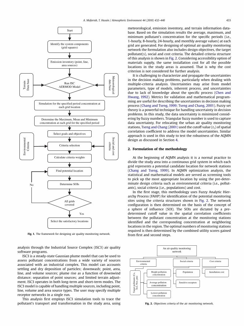
McElroy et al. (1986) applied air quality simulation models andpopulation exposure information to produce representativecombined patterns and then applied the concepts of ‘sphere ofinfluence’ (SOI) and ‘figure of merit’ (FOM) originally developed byLiu et al. (1986) to determine the minimum number of sitesrequired. To control the serious public health problems associatedwith the atmospheric pollution, the air quality protection authoritymust make the decisions by including environmental, social,economic and political criteria. This paper attempts to develop anobjective methodology considering the multiple-criteria, includingmultiple-pollutants concentration and social factors such as pop-ulation exposure and the construction cost. The framework of themethodology is shown in Fig. 1.

In this methodology, meteorological, emission inventory, andterrain database information is used to support the simulation

Start

Emission inventory (point, line, area sources)

each grid location

Ter

rain

D

ata

base

Determine the Maximum, Mean and Minimum concentration at each grid for the specified period

Simulation for the specified period concentration at

Identify the system components (grid squares)

Select goals and objectives

Criteria selection

Run ISC AERMOD Model

Meteorological data base

Calculate criteria weights

Find potential location

Social and cost criteria

Env

iron

men

tal

Cri

teri

a

Determine SOIs

All grids covered

Select the satisfactory locations

Yes

No

Fig. 1. The framework for designing air quality monitoring network.

An air quality monitoring network

Social criteriaEnvironmental criteria

Height pollutionconcentration

Average pollutionconcentration

Lowest pollutionconcentration

Population

Sensitive receptors

Installation cost

Cost criteria

Tar

get p

ollu

tant

s (C

o,

So2,

Nox

, pm

)

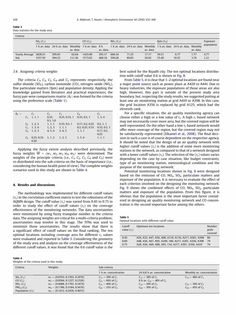
Fig. 2. Objectives criteria of the air monitoring network.

A. Mofarrah, T. Husain / Atmospheric Environment 44 (2010) 432–440 433

analysis through the Industrial Source Complex (ISC3) air qualitysoftware programs.

ISC3 is a steady-state Gaussian plume model that can be used toassess pollutant concentrations from a wide variety of sourcesassociated with an industrial complex. This model can accountssettling and dry deposition of particles; downwash; point, area,line, and volume sources; plume rise as a function of downwinddistance; separation of point sources; and limited terrain adjust-ment. ISC3 operates in both long-term and short-term modes. TheISC3 model is capable of handling multiple sources, including point,line, volume and area source types. The user may specify multiplereceptor networks in a single run.

This analysis first employs ISC3 simulation tools to trace thepollutant’s transport and transformation in the study area, using

meteorological, emission inventory, and terrain information data-base. Based on the simulation results the average, maximum, andminimum pollutant’s concentration for the specific periods (i.e.,1-hourly, 8-hourly, 24-hourly, and monthly average values) at eachgrid are generated. For designing of optimal air quality monitoringnetwork the formulation also includes design objectives, the targetpollutant(s), social and cost criteria. The detailed criteria structureof this analysis is shown in Fig. 2. Considering accessibility option ofmaterials supply, the same installation cost for all the possiblelocations in the study areas is assumed. That is why the costcriterion is not considered for further analysis.

It is challenging to characterize and propagate the uncertaintiesin the decision making problems, particularly when dealing withmultiple-criteria analysis. Uncertainties may arise from modelparameters, type of models, inherent process, and uncertaintiesdue to lack of knowledge about the specific process (Chen andHwang, 1992). Metrics for validation and mathematical program-ming are useful for describing the uncertainties in decision makingprocess (Chang and Tseng, 1999; Tseng and Chang, 2001). Fuzzy settheory is a powerful technique for handling uncertainty in decisionproblems. In this study, the data uncertainty is minimized consid-ering by fuzzy numbers. Triangular fuzzy number is used to capturedata uncertainty. For relocating the urban air quality monitoringstations, Tseng and Chang (2001) used the cutoff value (rc) of spatialcorrelation coefficient to address the model uncertainties. Similarapproach is used in this study to test the robustness of the AQMNdesign as discussed in Section 4.

2. Formulation of the methodology

At the beginning of AQMN analysis it is a normal practice todivide the study area into a continuous grid system in which eachgrid represents a potential candidate location for network stations(Chang and Tseng, 1999). In AQMN optimization analysis, thestatistical and mathematical models are served as screening toolsto pick up the most appropriate location by using the pre-deter-minate design criteria such as environmental criteria (i.e., pollut-ants), social criteria (i.e., populations) and cost.

In the first stage, this methodology uses Fuzzy Analytic Hier-archy Process (FAHP) for identification of the potential monitoringsites using the criteria structures shown in Fig. 2. The networkconfiguration is then determined on the basis of the concept ofa sphere of influence (SOI). The SOIs are dictated by a pre-determined cutoff value in the spatial correlation coefficientsbetween the pollutant concentration at the monitoring stationsidentified and the corresponding concentration at neighboringlocations in the region. The optimal numbers of monitoring stationsrequired is then determined by the combined utility scores gainedfrom first and second steps.

A. Mofarrah, T. Husain / Atmospheric Environment 44 (2010) 432–440434

2.1. Step 1: identification and ranking of potential monitoring sites

The four objectives are considered separately in this step:calculating scores of each criterion, assigning weighting factors tothe criteria, determining the utility scores by multiplying thecriteria scores with weighting factors and ranking the potentiallocation based on the utility scores.

2.1.1. Calculating scores of each criterionThe criteria data for each grid, like population, pollutant’s

concentration from the ISC3 model (i.e., 1-hourly 8-hourly and24-hourly average of a year) are normalized to unity by dividing themaximum data value within the group as shown in Equation (1).The minimum, average and maximum normalized scores are usedto generate triangular fuzzy numbers (TFNs).

Normalized value ¼ � Ci

Cmax(1)

where Ci is the criteria value and Cmax is the maximum value of thedata set.

2.1.2. Criteria weight computationSeveral weighting methods are used to determine the relative

importance of the criteria involved in the decision making process.The Analytic Hierarchy Process (AHP), which is a powerful tech-nique introduced by (Saaty, 1980), has proven to be useful instructuring complex multi-criteria decision making (MCDM)problems in engineering, economics and social science. Inconventional AHP, the pair-wise comparison matrix (PCM) isestablished using a nine-point scale that converts the humanpreferences between available alternatives. However, due tovagueness and uncertainty in the decision-maker’s judgment, theuse of crisp value may leads to uncertainties in the final results. Inthis study, the vagueness and uncertainty is handled by using thetriangular fuzzy number. The nine-point scale suggested by Saaty(1980) is fuzzified by triangular fuzzy number as shown in Table 1.

To demonstrate fuzzy AHP, a simple example is introduced here.Consider three criteria C1, C2 and C3. Using the fuzzy values(Table 1), the pair-wise comparisons matrix ðApcmÞ of these criteriais developed. According to the principle of the AHP, each element ofthe lower triangle in the PCM is reciprocal to the upper triangle (i.e.,Ijk ¼ 1/Ijk, where, Ijk is the component of the lower triangle in thePCM).

½C1 C2 C3 �"C1#" 1;1;1 1=5;1=2;1 1;1;1 #

Apcm ¼ C2C3

1;2;5 1;1;1 1=3;3;11;1;1 1;1=3;3 1;1;1

After constructing the fuzzy PCM, relative weights of eachcriterion is calculated by using fuzzy extent analysis (Lee et al.,2006) as follows:

Table 1Conversion of crisp PCM to fuzzy PCM.

How important is A relative to B? Preference index(Saaty, 1980)

Fuzzy value(l, m, u; Jie et al., 2006)

Equally important 1 (1, 1, 1)Moderately more important 3 (1, 3, 5)Strongly more important 5 (3, 5, 7)Very strongly more important 7 (5, 7, 9)Overwhelmingly more important 9 (7, 9, 11)Intermediate values

(Need to judge two)2 (1, 2, 4)4 (2, 4, 6)6 (4, 6, 8)8 (6, 8, 10)

Total sum of the whole fuzzy PCM:

Left ¼ 1 þ 1/5 þ 1þ1 þ 1þ1/3 þ 1þ1 þ 1 ¼ 7.5 (a1)Middle ¼ 1 þ 1/2 þ 1þ2 þ 1þ3 þ 1þ1/3 þ 1 ¼ 11.83 (b1)Right ¼ 1 þ 1þ1 þ 5þ1 þ 1þ1 þ 3þ1 ¼ 15.0 (c1)

The first row sum (for C1)

Left ¼ 1 þ 1/5 þ 1 ¼ 2.20 (a1)Middle ¼ 1 þ 1/2 þ 1 ¼ 2.5 (a2)Right ¼ 1 þ 1þ1 ¼ 3.0 (a3)

The corresponding weights (w1) for criterion C1 is as:

Left ¼ a1/c1 ¼ 2.2/15.0 ¼ 0.147Middle ¼ a2/b1 ¼ 2.50/11.83 ¼ 0.211Right ¼ a3/a1 ¼ 3/7.50 ¼ 0.40

Similarly the weights for the criteria C2 and C3 are (w2 ¼ 0.155,0.507, 0.934) and (w3 ¼ 0.200, 0.220, 0.667) respectively.

It is necessary to check the consistency of the develop matrixðApcmÞ. The consistency of the matrix ðApcmÞ can be checked bya consistency index (C.I) suggested by Saaty (1980) as:

C:I ¼ lmax � nn� 1

(2)

C:R ¼ C:IR:I

(3)

where C.I ¼ consistency index, C.R ¼ consistency ratio.lmax ¼ maximum eigenvalue, n ¼ number of parameters in thematrix, and R.I ¼ random index. Saaty (1980) suggested the R.Ivalues as in Table 2.

The threshold of the C.R less than 10% is assumed to be anadequate consistency. Since the components of ðApcmÞ are trian-gular fuzzy numbers (TFNs), the C.R can be evaluated only for themost likely value (Tesfamariam and Sadiq, 2006). For the mostlikely value of matrix ðApcmÞ, the maximum eigenvalue lmax wasfound 3.015; with n is equal to 3 produced C.I ¼ 0.008 andC.R ¼ 0.014, which is less than the 10% and that means the assignedcriteria weights are adequate consistency.

2.1.3. Determining the utility scoresIn this step, the grid systems are simplified by introducing

a single pattern score called air quality utility value (AQUV). Theresultant AQUVs are used to identify the most desirable moni-toring locations. The attractiveness of placing an air qualitymonitoring station at a given location is closely related to specificmonitoring objectives (Ludwig and Kealoha, 1975; Liu et al., 1977;and Ludwig et al., 1976). In general, the primary objective of an airquality monitoring network is to monitor the highest pollutantconcentrations in the area of interest to ensure compliance withair quality standards (Liu et al., 1986). To identify the potentialmonitoring site this study used the AQUV technique, which is theproduct sum of the criteria scores and the associated probabilitiesof occurrence as:

AQUV ¼XðCriteria scoresÞ � ðProbality of OccuranceÞ (4)

Table 2Random index values (Saaty, 1980).

N 1 2 3 4 5 6 7 8 9 10

R.I 0.0 0.0 0.58 0.9 1.12 1.24 1.32 1.41 1.45 1.49

A. Mofarrah, T. Husain / Atmospheric Environment 44 (2010) 432–440 435

The AQUV values in Equation (4) can be extended to designa multiple-criteria sources monitoring network by assigning therelative importance of the individual criteria (multiple-criteriameans multiple pollutants and other criteria like sensitive recep-tors, installation cost, traffic etc.). For example, to locate a site formeasuring multiple-criteria sources, the AQUV values in Equation(4) can be generalized using a composite air quality utility index(Ott and Thorn, 1976) as:

U ¼XN

i¼1

WiCi (5)

where U denotes the composite air quality utility index, Ci is thenormalized value of criteria i, and Wi is the correspondingweighting factor reflecting the importance of ith criteria. In general,Wi and Ci can be crisp or fuzzy data. However, due to vagueness anduncertainty in the decision-maker’s judgment, the use of crispvalues to assign weights may introduce subjective uncertainty,which can be addressed through assignment of fuzzy data. Forspecific locations Equation (5) can be generalized as:

+1

r

rc

-1 Distance (sc)

Fig. 3. The generalized correlation coefficient as a function of distance.

1 2 ...... nC C C

1 1 1 2 1 1

2 1 2 2 2 1Gi 1 2

1 2

.

....

. . . . .

.

A A nA

A A nAn

n An An nAn

A C C C

A C C C(6)U w w w

A C C C

where UGi is grid utility values, A1, A2,.., An are the possiblemonitoring station location, C1, C2,..,Cn are the normalizedcriteria scores to be considered for decision making purpose (fuzzyvalues) and w1, w2..wn is the corresponding fuzzy weightingfactor reflecting the importance of criteria.

2.1.4. Identification of the potential locationThe grid utility values (UGi) from Equation (6) are also fuzzy

values. For decision making purposes, the comparison of fuzzy datais not straightforward. The crisp value of a fuzzy set can be obtainedby different methods. Among the others, the centroidal indexmethod (Yager, 1980) is most widely applied approach for fuzzy setranking used in this study. The Yager (1980) centroid index isa geometric centre of the fuzzy number of alternative Ai, wheregeometric centre corresponds to an x value on the horizontal axis X.For a given TFN (a1, b1, g1), Yager’s (1980) centroid index as follows:

RxðAiÞ ¼ðb1�a1Þða1þ2=3ðb1�a1ÞÞþðl1�b1Þðb1þ1=3ðl1�b1ÞÞ

ðb1�a1Þþðl1�b1Þ(7)

where Rx (Ai) is a geometric centre of a fuzzy number of alternativeAi on the horizontal axis X and a1, b1, and g1 are the TNFs.Depending on the Rx (Ai) values the grid’s location can be ranked.For this study, the top 100 potential grid locations are selected forsecond step analysis.

2.2. Step 2: determination of spheres of influence

Once the potential monitoring location is decided, the secondstep is to determine the special area coverage of the monitoringstation. The special area coverage of the monitoring station isdetermined on the basis of the concept of a sphere of influence(SOI) suggested by Liu et al. (1986). SOI is defined as the zone overwhich the air quality data for a given monitoring location can beconsidered representative (Elkamel et al., 2008). The SOIs aredictated by a cutoff value (rc) in the spatial correlation coefficients

(r) between the pollutant concentrations at the monitoring loca-tions identified and the corresponding concentrations at neigh-boring locations in the region.

In this methodology, the special area coverage of the monitoringstation is determined on the basis of the concept of a sphere ofinfluence (SOI) suggested by Liu et al. (1986). SOI is defined as thezone over which the air quality data for a given monitoring locationcan be considered representative. The spatial correlation coefficient(r) can be used to represent the SOI. This coefficient gives an indi-cation of the relationship among the monitoring locations to beselected in the designed optimal monitoring network (Elkamelet al., 2008). The computation of spatial correlation coefficients (r)is carried out surrounding each potential station evaluated in step 1in all radial direction until the (r) falls below the predeterminedcutoff value (rc). The correlation coefficient (r), lies between�1 andþ1. The spatial correlation coefficient is decreased from 1 as thedistance increases (Liu et al., 1986). A cutoff distance (sc) can befound for a predetermined cutoff value (rc) as illustrated in Fig. 3. Inthis paper, the zone of representative candidate location isconsidered the area surrounding it in which the special correlationcoefficient (r) of this location with the nearby locations is higherthan the cutoff value (rc). This means the air quality data measuredat this location are representatively correlated with a certaindegree of confidence to any location in the network within the area.Fig. 4 illustrates the general concept of representative zone. By theconcept of a representative zone it was assumed that, whena station is installed in a grid square (i.e., A5), the nearby gridsquares (i.e., A1,.,A9) are marked as on Fig. 4 will not be allowed tobe installed with the same class of station. When searching for thenext station location, the marked grid squares are skipped,enhancing the solution searching efficiency.

For example, two adjacent monitoring locations x1 ¼ (x11,x12,.,x1n) and x2 ¼ (x21, x22,.,x2n) denote the pollutant concen-trations at the monitoring site x1 and the corresponding pollutantconcentrations at the neighboring monitoring station x2, respec-tively. Then the spatial correlation coefficient (r) for a sample size ncan be expressed as:

r ¼

Xn

i¼1

ðx1i � x1Þðx2i � x2ÞffiffiffiffiffiffiffiffiffiffiffiffiffiffiffiffiffiffiffiffiffiffiffiffiffiffiffiffiffiffiffiffiffiffiffiffiffiffiffiffiffiffiffiffiffiffiffiffiffiffiffiffiffiffiffiffiffiffiffiffiXn

i¼1

ðx1i � x1Þ2Xn

i¼1

ðx2i � x2Þ2vuut

(8)

where x1 ¼ 1n

Pni¼1 x1i and x2 ¼ 1

n

Pni¼1 x2i are the average

concentrations at location 1 and 2, respectively. When the SOI fora monitoring station is calculated, the coverage area of the sphere isdefined as the number of monitoring site places inside it. Thecoverage area of each potential location can be quantified in termsof grid scores. A grid score Ugi for an ith candidate location isdefined as the number of grids correlated with this location, abovethe specified cutoff values (rc) as shown in Equation (9).

Fig. 4. Representative zone locations.

Fig. 5. Study area showing the

A. Mofarrah, T. Husain / Atmospheric Environment 44 (2010) 432–440436

Ugi ¼ maximizeXp

n (9)

j¼1

where n is the number of grids covered by a potential location i, andp is the type of pollutants (p ¼ 1, 2,., p). Finally, the optimum airmonitoring location is determined by total utility scores as:

UðTiÞ ¼Xmj¼1

Ugi � UGi

The higher utility scores U(Ti) mean the best location for the airquality monitoring network.

3. Case study

3.1. Background

The Riyadh city has a refinery, power plant, and cementindustry. The population of the city is above 4 million with veryhigh growth rates. Therefore, to maintain the air quality standardthe city authorities plan to re-assess and expand the current airquality monitoring network. There are six existing air quality

existing stations location.

0

100000

200000

300000

400000

500000

600000

700000

PM SO2 NOx COPollutants

(tonn

es/y

ear)

Point sources ton/y

Line sources ton/y

Area sources ton/y

Fig. 6. Emissions of each pollutant in the Riyadh city.

A. Mofarrah, T. Husain / Atmospheric Environment 44 (2010) 432–440 437

monitoring stations in the Riyadh city owned and operated bydifferent organizations. The locations of the existing air qualitymonitoring stations are shown in Fig. 5. The main objective of thisstudy is to review the existing monitoring network and to identifythe optimal station locations for the extended air quality moni-toring network by applying the proposed methodology.

3.2. Emission inventory

The emission inventory for Riyadh city was compiled consid-ering the three major emission sources such as point sources, areasources and line sources. The major point sources in the Riyadh cityare power plants, refinery and cement industry. The old and newindustrial cities under development are considered as the area

Fig. 7. Relative distribution of each pollutan

source. The automobile sources for the selected major roads basedon traffic counts, composition of traffic, and model years wereconsidered as the line sources in this study. The database for pointand area source emission inventory was developed on the basis ofproduction rate, fuel consumption and available control tech-nology. For line sources, the emission factors as suggested by U.S.EPA were used. Fig. 6 compares the emissions of each targetpollutant in the Riyadh city.

The relative contribution by source category to emissions of PM,SO2, CO, and NOx, is categorized by point, line, and area sources.Fig. 7 illustrates the relative distribution of each pollutant by sourcecategory. In particular, point and area sources contribute 17% and80% of the total PM emissions, respectively. In the case of SO2, pointsource is the largest contributor, accounting for nearly 89% of allSO2 emissions. Mobile sources rank highest in contributions to COemissions. The percent contribution of mobile sources to CO isabout 99%.

3.3. Optimization of the network

At the beginning of this analysis, the study area (Fig. 5) wasconceptually divided into square grids as subsystems. Each gridsquare was set as 2.0 km by 2.5 km. The grid component includedair pollutants sources (i.e., the industry, mobile and area sources)and social objectives (i.e., the number of exposure population). Thetotal air pollution emission quantity in each square grid wascalculated as the sum of the emission quantity of the point, line,and area sources. The air pollutants considered in this studyincluded sulfur dioxide (SO2), nitrogen oxide (NOx), carbonmonoxide (CO) and fine particulate matters (fpm). The concentra-tion level of each pollutant was simulated on hourly, 8-hourly and24-hourly basis using ISC3 model. Population data of each gridwere also collected. The input data statistics for this study isreported in Table 3. The data of each criterion was then normalizedto unity by Equation (1). The minimum, average and maximumnormalized scores were used to generate TFNs.

t by source category in the Riyadh city.

Table 3Data statistics for the study area.

Criteria

SO2 (C1) CO (C2) NOx (C3) fpm (C4) Exposurepopulation

1 h av. data 24 h av. data Monthlyav. data

1 h av. data 8 hav. data

1 h av. data 24 h av. data Monthlyav. data

1 h av. data 24 h av. data Monthlyav. data

Yearly Average 2828.51 295.65 62.64 1425.90 395.17 666.34 71.25 17.17 59.51 6.77 1.77 4.77Std. 3357.95 504.33 111.36 1573.03 468.18 599.28 89.85 20.92 55.49 10.35 3.76 1.21

A. Mofarrah, T. Husain / Atmospheric Environment 44 (2010) 432–440438

3.4. Assigning criteria weights

The criteria C1, C2, C3, C4 and C5 represents respectively, thesulfur dioxide (SO2), carbon monoxide (CO), nitrogen oxide (NOx),fine particulate matters (fpm) and population density. Appling theknowledge gained from literature and practical experiences, thefuzzy pair-wise comparisons matrix ð~AFÞwas formed for the criteriausing the preference scale (Table 1).

~AF ¼ C1 C2 C3 C4 C5

C1 1, 1, 1 0.33,0.5, 1.0

0.25, 0.33, 1 0.33, 0.5, 1 1, 3, 4

C2 1, 2, 3 1, 1, 1 0.33, 0.5, 1 0.17, 0.2, 0.25 0.5, 1, 1C3 1, 3, 4 1, 2, 3 1, 1, 1 0.2, 0.25, 0.33 0.33, 0.5, 1C4 1, 2, 3 4, 5, 6 3, 4, 5 1, 1, 1 0.17, 0.2,

0.25C5 0.25, 0.33,

0.501, 1, 2 1, 2, 3 1, 5, 6 1, 1, 1

Applying the fuzzy extent analysis described previously, thefuzzy weights W ¼ ðw1;;w2;w3;w4;w5Þ were determined. Theweights of the principle criteria (i.e., C1, C2, C3, C4 and C5) werere-distributed into the sub-criteria on the basis of importance (i.e.,considering the human health point of view). The complete weightsscenarios used in this study are shown in Table 4.

Table 5Optimal locations with different cutoff value.

Cutoffvalue (rc)

Optimum ten locations Numbergridscovered

0.45 A26, A32, A47, A56, A98, A110, A116, A217, A301, A398 860.60 A48, A56, A67, A95, A109, 180, A217, A301, A356, A398 790.75 A28, A56, A69, A88, A95, 134, A217, A301, A356, A419 74

4. Results and discussions

The methodology was implemented for different cutoff values(rc) in the correlation coefficient matrix to test the robustness of theAQMN design. The cutoff value (rc) was varied from 0.45 to 0.75 inorder to study the effect of cutoff values (rc) on the coverageeffectiveness of the monitoring networks. The data uncertaintieswere minimized by using fuzzy triangular number in the criteriadata. The assigning weights are critical for a multi-criteria problem;uncertainties may involve in this stage. The TFNs was used tominimize those uncertainties. The results show that there isa significant effect of cutoff values on the final ranking. The tenoptimal locations including coverage area for different rc valueswere evaluated and reported in Table 5. Considering the geometryof the study area and analysis on the coverage effectiveness of thedifferent cutoff values, it was found that the 0.6 cutoff value is the

Table 4Weights of the criteria used in this study.

Criteria Weights Sub-criteria

1 h av. concentra

SOx (C1) w1 ¼ (0.0763, 0.1393, 0.2978) C11 ¼ 30% of C1

CO (C2) w2 ¼ (0.0584, 0.1227, 0.2326) C21 ¼ 60% of C2

NOx (C3) w3 ¼ (0.0688, 0.1762, 0.3474) C31 ¼ 40% of C3

PM10 (C4) w4 ¼ (0.1786, 0.3184, 0.5676) C41 ¼ 25% of C4

Population (C5) w5 ¼ (0.1412, 0.2436, 0.4653)

best suited for the Riyadh city. The ten optimal locations distribu-tion with cutoff value 0.6 is shown in Fig. 8.

From Table 5, it is clear that 1–2 optimal locations are found neara major point source such as power plant at A420 to A441. Due toheavy industries, the exposure populations of those areas are alsohigh. However, this part is outside of the present study areaboundary, but, respecting the study results, we suggested putting atleast one air monitoring station at grid A419 or A398. In this case,the grid location A356 is replaced by grid A125, which had theeleventh rank.

For a specific situation, the air quality monitoring agency canchoose either a high or a low value of rc. A high rc based networkmay not necessarily cover more area, but the covered region will bewell represented. On the other hand a low rc based network wouldoffer more coverage of the region, but the covered region may notbe satisfactorily represented (Elkamel et al., 2008). The final deci-sion in such a case is of course dependent on the respective agency.It should be noted that the design of an air quality network withhigher cutoff values (rc) is the addition of some more monitoringstations in the network, as compared to that of a network designedwith a lower cutoff values (rc). The selection of the (rc) values variesdepending on the case by case situation, like budget constraints,type of air monitoring station, meteorological condition and thepurpose of the monitoring network.

Potential monitoring locations shown in Fig. 8 were designedbased on the emission of CO, NOx, SO2, particulate matters andexposure of the population. It is necessary to evaluate the effect ofeach criterion involved on the designing the monitoring network.Fig. 9 shows the combined effects of CO, NOx, SO2, particulatematters and exposure of the population. From this figure, it isobvious that the population is the most important factor consid-ered in designing air quality monitoring network and CO concen-tration is the second important factor among the others.

tion 24 h/8 h av. concentration Monthly av. concentration

C12 ¼ 30% of C1 C13 ¼ 40% of C1

8 h av. C22 ¼ 40% of C2

C32 ¼ 30% of C3 C33 ¼ 30% of C3

C42 ¼ 30% of C4 C43 ¼ 45% of C4

Fig. 8. Location of the ten optimal stations (for cutoff value 0.6).

0%

10%

20%

30%

40%

50%

60%

CO Sox Nox fpm populationCriteria

Percen

tag

e effects

Fig. 9. Effect analyses of the major criteria involved in designing air monitoringstations.

A. Mofarrah, T. Husain / Atmospheric Environment 44 (2010) 432–440 439

5. Conclusions

The AQMN represents an essential tool to monitor and controlatmospheric pollution. The use of some specific criteria inconjunction with the mathematical models provides a generalapproach to determine the optimal number and location of moni-toring stations. In this study, a multiple-criteria approach inconjunction with the special correlation technique was used todevelop optimal AQMN design. The triangular fuzzy numbers(TFNs) were used to capture the uncertain (i.e., assigning weights)

components in the decision making process. The special areacoverage of the monitoring station is an essential part of an AQMN,which was determined on the basis of the concept of a sphere ofinfluence. The effect of the correlation coefficient as well as thecutoff values on coverage of the network was also studied bychanging the cutoff values.

Finally, this methodology was structured to provide theassessment of AQMN design in a specific case. The design of anAQMN is not simple or straightforward and depends on many site-specific issues and the purposes. Good upfront planning is thereforecrucial in properly assessing the problem and designing an optimalAQMN.

Acknowledgement

Financial support provided by the Natural Science and Engi-neering Research Council of Canada (NSERC) is highly appreciated.

References

Chang, N.B., Tseng, C.C., 1999. Optimal design of multi-pollutant air quality moni-toring network in a Metropolitan region using Kaohsiung, Taiwan as anexample. Journal of Environmental Monitoring and Assessment 57 (2), 121–148.

Chen, S.J., Hwang, C.L., 1992. Fuzzy Multiple Attribute Decision-Making. Springer-Verlag, New York.

Elkamel, A., Fatehifar, E., Taheri, M., Al-Rashidi, M.S., Lohi, A., 2008. A heuristicoptimization approach for Air Quality Monitoring Network design with thesimultaneous consideration of multiple pollutants. Environmental Manage-ment 88, 507–516.

Egmond, N.D.V., Onderdelinden, D., 1981. Objective analysis of air pollution moni-toring network data: spatial interpolation and network density. AtmosphericEnvironment 15 (6), 1035–1046.

A. Mofarrah, T. Husain / Atmospheric Environment 44 (2010) 432–440440

Graves, R.J., Lee, T.D., McGinnis, L.F.J., 1981. Air Monitoring Network Design: casestudy. Journal of Environmental Engineering: ASCE 107 (5), 941.

Handscombe, C.M., Elson, D.M., 1982. Rationalisation of the National Survey of AirPollution Monitoring Network of the United Kingdom using spatial correlationanalysis: a case study of the Greater London area. Atmospheric Environment 4B(3), 395.

Jie, H.L., Meng, M.C., Cheong, C.W., 2006. Web based fuzzy multicriteria decisionmaking tool. International Journal of the Computer, the Internet and Manage-ment 14 (2), 1–14.

Koda, M., Seinfeld, J.H., 1978. Air Monitoring Siting by Objective. EPA-600/4-7-036.U.S. Environmental Protection Agency, Las Vegas, Nevada.

Lee, H.J., Meng, M.C., Cheong, C.W., 2006. Web based fuzzy multicriteria decisionmaking tool’. International Journal of the Computer, the Internet andManagement 14 (2), 1–14.

Ludwig, F.L., Berg, N.J., Hoffman, A.J., 1976. The selection of sites for air pollutantmonitoring. Paper presented at the 69th Annual Meeting of the Air PollutionControl Association, Portland, Oregon.

Ludwig, F.L., Kealoha, J.H.S., 1975. Selecting Sites for Carbon Monoxide Monitoring.EPA 450/3-75-077. U.S. Environmental Protection Agency, Research TrianglePark, North Carolina.

Liu, M.K., Avrin, J., Pollack, R.I., Behar, J.V., McElory, J.L., 1986. Methodology fordesigning air quality monitoring networks. Environmental Monitoring andAssessment 6, 1–11.

Liu, M.K., Meyer, J., Pollack, R., Roth, P.M., Seinfeld, J.H., Behar, J.V., Dunn, L.M.,McElroy, J.L., Lena, P.N., Pitchford, A.M., Fisher, N.T., 1977. Development ofa Methodology for the Design of a Carbon Monoxide Monitoring Network. EPA-600/4-77-019. U.S. Environmental Protection Agency, Las Vegas, Nevada.

McElroy, J.L., Behar, J.V., Meyers, T.C., Liu, M.K., 1986. Methodology for designing AirQuality Monitoring Networks: II. Application to Las Vegas, Nevada, for carbonmonoxide. Environmental Monitoring and Assessment 6, 13.

Modak, P.M., Lohani, B.N., 1985. Optimization of ambient Air Quality MonitoringNetworks: part I. Environmental Monitoring and Assessment 5, 1–19.

Ott, W.R., Thorn, G.C., 1976. A critical review of air pollution index systems in theUnited States and Canada. Journal of the Air Pollution Control Association 26,460–470.

Pickett, E.E., Whiting, R.G., 1981. The design of cost-effective Air Quality MonitoringNetworks. Environmental Monitoring and Assessment 1, 59.

Saaty, T.L., 1980. The Analytic Hierarchy Process. McGraw-Hill, New York.Tesfamariam, S., Sadiq, R., 2006. Risk-based environmental decision-making using

fuzzy analytic hierarchy process (F-AHP). Stochastic Environmental Researchand Risk Assessment 21, 35–50.

Tseng, C.C., Chang, N.B., 2001. Assessing relocation strategy of urban air qualitymonitoring network by compromise programming. Environment International26, 524–541.

Yager, R.R., 1980. On a general class of fuzzy connectives. Fuzzy Sets and Systems 4,235–242.