JHEP12(2013)086 Published for SISSA by Springer Received: November 2, 2013 Accepted: December 4, 2013 Published: December 19, 2013 A holographic model of the Kondo effect Johanna Erdmenger, a Carlos Hoyos, b Andy O’Bannon c,d and Jackson Wu e a Max-Planck-Institut f¨ ur Physik (Werner-Heisenberg-Institut), F¨ohringer Ring 6, 80805 M¨ unchen, Germany b Raymond and Beverly Sackler School of Physics and Astronomy, Tel-Aviv University, Ramat-Aviv 69978, Israel c Department of Applied Mathematics and Theoretical Physics, University of Cambridge, Cambridge CB3 0WA, U.K. d Rudolf Peierls Centre for Theoretical Physics, University of Oxford, 1 Keble Road, Oxford OX1 3NP, U.K. e National Center for Theoretical Sciences, Physics Division, No. 101, section 2, Kuang Fu Road, Hsinchu, Taiwan 300, R.O.C. E-mail: [email protected], [email protected], [email protected], [email protected]Abstract: We propose a model of the Kondo effect based on the Anti-de Sitter/Conformal Field Theory (AdS/CFT) correspondence, also known as holography. The Kondo effect is the screening of a magnetic impurity coupled anti-ferromagnetically to a bath of conduc- tion electrons at low temperatures. In a (1+1)-dimensional CFT description, the Kondo effect is a renormalization group flow triggered by a marginally relevant (0+1)-dimensional operator between two fixed points with the same Kac-Moody current algebra. In the large- N limit, with spin SU(N ) and charge U(1) symmetries, the Kondo effect appears as a (0+1)-dimensional second-order mean-field transition in which the U(1) charge symmetry is spontaneously broken. Our holographic model, which combines the CFT and large-N descriptions, is a Chern-Simons gauge field in (2+1)-dimensional AdS space, AdS 3 , dual to the Kac-Moody current, coupled to a holographic superconductor along an AdS 2 sub- space. Our model exhibits several characteristic features of the Kondo effect, including a dynamically generated scale, a resistivity with power-law behavior in temperature at low temperatures, and a spectral flow producing a phase shift. Our holographic Kondo model may be useful for studying many open problems involving impurities, including for example the Kondo lattice problem. Keywords: Holography and condensed matter physics (AdS/CMT), Gauge-gravity cor- respondence, AdS-CFT Correspondence ArXiv ePrint: 1310.3271 c SISSA 2013 doi:10.1007/JHEP12(2013)086
Transcript
JHEP12(2013)086
Published for SISSA by Springer
Received: November 2, 2013
Accepted: December 4, 2013
Published: December 19, 2013
A holographic model of the Kondo effect
Johanna Erdmenger,a Carlos Hoyos,b Andy O’Bannonc,d and Jackson Wue
2.1.2 Leading irrelevant operator and low-T scalings 9
2.2 Large-N techniques 11
3 Top-down holographic model 12
3.1 The D7-branes 13
3.2 The D5-branes 15
3.3 The Kondo coupling 17
4 Bottom-up holographic model 20
4.1 Asymptotics and boundary terms 23
4.2 Stability analysis 25
4.3 The phase transition 29
4.4 The IR fixed point 31
4.4.1 The leading irrelevant operator 32
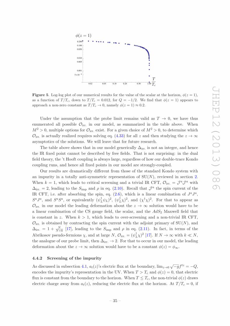
4.4.2 Screening of the impurity 35
4.4.3 The phase shift 36
5 Summary and outlook 40
1 Introduction and summary
The Kondo effect [1] is the screening at low temperatures T of a magnetic moment coupled
anti-ferromagnetically to a bath of conduction electrons. The Kondo interaction involves
only the spins of the magnetic impurity and the electrons, both of which are spin-1/2
representations of the SU(2) spin symmetry. Heuristically, the screening occurs when an
electron becomes bound to the impurity, forming the so-called Kondo singlet, below a
characteristic, dynamically-generated scale, the Kondo temperature TK . More precisely,
the screening occurs when a many-body resonance forms, the Kondo resonance. The Kondo
effect has been observed in many systems, the canonical examples being metals doped with
magnetic ion impurities [2, 3] and quantum dots [4–6]. A key experimental signature of
the Kondo effect appears in the resistivity, ρ, which behaves as − ln (T/TK) in the regime
T ≫ TK [1].
– 1 –
JHEP12(2013)086
The theory of the Kondo effect employs many techniques, including Wilson’s numer-
ical renormalization group (RG) [7], Nozieres’ Fermi liquid description [8, 9], the Bethe
Ansatz [10–14], large-N limits [14–17], conformal field theory (CFT) [18–23], and others.
For reviews of many of these, see refs. [24, 25]. Taken together, these techniques provide
complete information about the spectrum, thermodynamics, and transport properties of
the Kondo system at all energy scales. The single-impurity Kondo problem is thus consid-
ered a solved problem.
Many open questions remain about the Kondo effect, however. For example, an impor-
tant unsolved problem is the generalization from a single impurity to multiple impurities
with Ruderman-Kittel-Kasuya-Yosida (RKKY) interactions among one another, which can
promote anti-ferromagnetic ordering of the impurity spins [26]. Many heavy fermion com-
pounds realize a dense lattice of magnetic moments, i.e. a “Kondo lattice,” wherein a
competition between the Kondo and RKKY interactions gives rise to a quantum phase
transition [26–30]. The quantum critical degrees of freedom subsequently give rise to non-
Fermi liquid behavior, namely the “strange metal” state with resistivity ρ ∝ T [30]. Various
obstacles have prevented a solution of the Kondo lattice problem (in more than one spatial
dimension [27]). For example, even with just two impurities, integrability is lost. More-
over, the quantum critical degrees of freedom are strongly coupled. Other important open
questions involve entanglement entropy [31] and far-from-equilibrium evolution [32, 33] of
Kondo systems, both of which are difficult to study using the techniques mentioned above.
With an eye towards these (and other) open questions, our goal is to apply a new tech-
nique to the Kondo problem: the Anti-de Sitter/CFT Correspondence (AdS/CFT), also
known as gauge-gravity duality or holography [34–36]. AdS/CFT equates a weakly-coupled
theory of gravity in (d+1)-dimensional AdS spacetime, AdSd+1, with a strongly-coupled
d-dimensional CFT “living” on the AdS boundary. In the best-understood examples the
CFT is a non-Abelian Yang-Mills (YM) theory in the ’t Hooft large-N limit.
Holographic models come in two kinds: top-down and bottom-up. Top-down models
are obtained from string theory constructions, while bottom-up models are ad hoc toy
models that may or may not descend from an ultra-violet (UV)-complete string theory.
Various holographic Kondo models have been proposed, most of them top-down, with a
strongly-coupled non-Abelian YM theory playing the role of the electrons, the SU(N) gauge
group playing the role of the spin symmetry, and a Wilson line operator playing the role
of the impurity [37–49].1 Some basic phenomena of the Kondo effect are missing from
these top-down models, however, a prominent example being the dynamically-generated
scale TK .
Our goal is to find a bottom-up holographic Kondo model, with simple, generic ingre-
dients that might be useful for further model building. We consider only a single impurity.
Our strategy is in fact to consider a new top-down model with symmetries closer to those of
actual Kondo systems. We then identify the minimal, essential ingredients of the top-down
model to motivate a bottom-up model. We perform calculations only in our bottom-up
model, to demonstrate that the model indeed captures some basic Kondo physics.
1See also ref. [50] for an attempt to translate the Kondo Hamiltonian to holography directly, using a
multi-scale entanglement renormalization ansatz, in the spirit of refs. [51, 52].
– 2 –
JHEP12(2013)086
We employ the CFT and large-N approaches to the Kondo effect. The CFT ap-
proach [18–23] begins by reducing the problem to one spatial dimension. The key step is a
partial wave decomposition of the electrons, retaining only the s-wave. The resulting effec-
tive theory is simply free chiral fermions in one dimension, which is a (1+1)-dimensional
CFT with a Kac-Moody current algebra. Solving the Kondo problem then reduces to an
exercise in Kac-Moody algebra representation theory, namely, determining how representa-
tions re-arrange between UV and infra-red (IR) fixed points. The large-N approach [14–17]
begins by generalizing the SU(2) spin group to SU(N), followed by a standard vector-like
large-N limit. If we write the impurity’s spin operator as a bi-linear in auxiliary “slave”
fermions, then the Kondo coupling is double-trace with respect to SU(N), and the Kondo
effect appears as “superconductivity” at the location of the impurity [14, 15, 53, 54]: a
(0+1)-dimensional charged scalar operator condenses at a critical temperature Tc near TK .
The charged scalar is built from an electron and a slave fermion, and its condensation
represents the formation of the Kondo singlet. Crucially, the large-N limit is only reliable
for low T [14–17, 24], essentially because the impurity can only affect observables when
T ≤ Tc. In particular, the characteristic − ln (T/TK) contribution to ρ at T ≫ TK does
not appear at leading order in the large-N limit.
Our top-down model begins with (3+1)-dimensional N = 4 supersymmetric YM theory
(SYM) with gauge group SU(Nc), in the large-Nc limit and with large ’t Hooft coupling.
We then introduce chiral fermions in the fundamental representation of SU(Nc) localized to
a (1+1)-dimensional defect. Our chiral fermions do not come from an s-wave reduction, but
they do realize a Kac-Moody current algebra. They are also our new ingredient, compared
to the earlier holographic models [37, 39, 41–49]. We introduce the impurity as a Wilson
line of SU(Nc) described by (0+1)-dimensional slave fermions. The holographic dual of
N = 4 SYM in the limits above is type IIB supergravity in AdS5 × S5 [34]. The chiral
fermions are dual to D7-branes along AdS3 × S5 [55–58] while the slave fermions are dual
to D5-branes along AdS2 × S4 [55, 59–62]. We consider coincident D7- and D5-branes,
which we treat as probes, neglecting their back-reaction on supergravity fields.
The probe D-brane actions reveal the essential ingredients for our holographic model.
The D7-brane action includes a Chern-Simons (CS) gauge field in the AdS3 part of its
worldvolume, dual to a current obeying a Kac-Moody algebra [63–67]. The D5-brane
action includes a YM gauge field in the AdS2 part of the worldvolume whose electric flux
encodes the representation of the Wilson line [61, 62]. Open strings between the D7- and
D5-branes give rise to a complex scalar bi-fundamental under the two gauge fields and
localized to the intersection of the D-branes, AdS2 × S4. The dual scalar operator is built
from the chiral and slave fermions, and the double-trace Kondo coupling appears in the bulk
through a special boundary condition on the scalar [68, 69]. We do not know the potential
for the scalar in our top-down model, but having identified the essential ingredients we can
proceed to our bottom-up model.
Our bottom-up model consists of an AdS3 CS gauge field, an AdS2 YM field, and a
bi-fundamental AdS2 scalar with a non-zero mass but no self-interactions. We introduce
a black hole in AdS3 with Hawking temperature T and introduce electric flux of the AdS2YM field. We show analytically that at low T the trivial solution for the scalar is unstable
– 3 –
JHEP12(2013)086
because of the special boundary condition. We then construct non-trivial solutions numer-
ically, which exist only because of the special boundary condition [70]. By computing the
free energy and condensate numerically, we demonstrate that a second-order mean-field
phase transition occurs from the trivial solution to a non-trivial solution as T decreases. In
short, our system is a holographic superconductor in AdS2 [71, 72]. In field theory terms,
a (0+1)-dimensional charged scalar operator condenses due to the double-trace Kondo
coupling, as expected.
In holography the AdS radial coordinate is dual to the field theory’s RG scale. Our
non-trivial scalar solution is thus the holographic representation of an RG flow between two
fixed points. In contrast, most previous holographic Kondo models described only fixed
points [41, 42, 44–49]. To be clear, our field theory has two couplings, the single-trace ’t
Hooft coupling and the double-trace Kondo coupling. We work in the probe limit, so the
’t Hooft coupling does not run, and is always large. As a result, any fixed points in our
model are necessarily strongly-coupled. On the other hand, we will demonstrate that our
Kondo coupling runs in a way similar to that in the original Kondo system.
We do not find a − ln (T/TK) contribution to ρ when T ≫ TK , due to the large-
N limit, as mentioned above. We do find many of the other “smoking gun” phenomena
characteristic of the Kondo effect, however, including:
• Dynamical scale generation: a holographic calculation in our model reveals that our
double-trace Kondo coupling diverges at a dynamically-generated scale, our TK . We
also find that Tc is on the order of TK .
• Power-law scalings at low T : we will argue that in our model, the entropy, resistivity,
and other observables exhibit power law behavior in T when T ≪ Tc, with the powers
of T fixed by the dimension of the leading irrelevant operator when we deform about
the IR fixed point. In our model that dimension is non-integer, indicating a non-
trivial IR fixed point, as expected, given the large ’t Hooft coupling.
• Screening of the impurity: in our model, when T ≤ Tc the non-trivial scalar draws
electric flux away from the AdS2 YM field deep in the bulk of AdS2. The reduced
electric flux deep in the bulk represents an impurity in a lower-dimensional represen-
tation of SU(Nc) in the IR. In other words, the impurity is screened in the IR.
• Phase shift: as we review in section 2, the Kondo effect produces a phase shift for
the electrons at the IR fixed point. In our model, when T ≤ Tc the non-trivial bi-
fundamental scalar transfers electric flux from the AdS2 YM field to the CS gauge
field, generating a Wilson loop for the CS gauge field deep in the bulk of AdS3,
which leads to a phase shift for the chiral fermions (our electrons) at the IR fixed
point [64, 65].
In short, our model captures much of the essential physics of the large-N , single-
impurity Kondo effect. We hope that our model may be useful for studying the many open
problems about the Kondo effect, especially those for which holography is particularly
well-suited, such as entanglement entropy and far-from-equilibrium phenomena.
– 4 –
JHEP12(2013)086
This paper is organized as follows. In section 2 we review the CFT and large-N
approaches to the Kondo problem. In section 3 we present our top-down model. In section 4
we present our bottom-up model, and present all of the results mentioned above. We end
in section 5 with a summary and a discussion of future research directions.
2 Review of the Kondo effect
The literature about the Kondo effect is enormous. In this section we will very briefly
review only those subjects essential to the construction of our holographic model.
The Kondo effect occurs when a magnetic impurity is coupled to free electrons, or
more precisely, a Landau Fermi liquid (LFL) of electrons. The Kondo Hamiltonian density
is [1]
HK = ψ†α
−∇2
2mψα + λK δ(~x) ~S · ψ†
α′
1
2~τα′α ψα, (2.1)
where the first term is the electron kinetic term and the second term represents the interac-
tion between the electrons and the impurity. Here ψ†α and ψα are creation and annihilation
operators for an electron of spin α =↑ or ↓, i.e. the electrons are in the fundamental repre-
sentation of the spin SU(2) symmetry, ∇2 is the Laplacian of flat R3, m is the electron mass,~S is the spin of the impurity, which is also in the fundamental representation of SU(2), ~τ is
the vector of Pauli matrices, and λK is the Kondo coupling. Anti-ferromagnetic coupling
means λK > 0, ferromagnetic means λK < 0.
The leading-order perturbative result for λK ’s beta function is negative. As a result,
when λK < 0, the effective coupling goes to zero at low energy. When λK > 0, however,
the system exhibits asymptotic freedom, a dynamically generated scale, TK , and a coupling
that appears to diverge at low energy, leading to the Kondo problem: what is the ground
state of the Kondo Hamiltonian when λK > 0?
As mentioned in section 1, the single-impurity Kondo problem has been solved using
a combination of complementary techniques. The solution is usually expressed in terms of
an RG flow from a UV fixed point to an IR fixed point. Thanks to asymptotic freedom,
the UV fixed point is a LFL and a decoupled spin. As we flow to lower energy, the ground
state changes at the scale TK . Heurstically, an electron becomes bound to the impurity,
their spins combining into an anti-symmetric singlet of SU(2), the Kondo singlet. More
precisely, a many-body resonance, the Kondo resonance, forms, and the impurity spin is
screened. The change in the ground state is a crossover, not a phase transition. At the
IR fixed point the spin is absent, having been completely screened, while the remaining,
unbound electrons form a LFL with a special boundary condition: the electronic wave
function vanishes at the impurity’s location. Intuitively, the reason is that any electron
that attempts to penetrate that location must break apart the Kondo singlet, which has a
very large binding energy, ∝ λK , making such events energetically costly and so extremely
unlikely. The special boundary condition means that the IR spectrum is shifted relative to
the UV, i.e. some spectral flow occurs. In short, although from the perspective of the UV
degrees of freedom λK diverges in the IR, the IR degrees of freedom arrange themselves
into a LFL with a special boundary condition.
– 5 –
JHEP12(2013)086
The Kondo Hamiltonian admits several generalizations. We can promote spin SU(2)
to SU(N), and we can consider multiple channels, or in particle physics language multiple
flavors, of electrons. With k channels, the total symmetry is SU(N) × SU(k) × U(1),
with SU(k) and U(1) the channel and charge symmetries, respectively. By definition,
the electrons are in the fundamental of SU(N) × SU(k) and the impurity is a singlet of
SU(k) × U(1). A Kondo Hamiltonian is thus specified by three data: N , k, and the
representation of the impurity under SU(N). These generalizations are relevant for real
systems, including quantum dots and some alloys: in some cases the impurity has a large
spin degeneracy, so N > 2, and/or multiple conduction bands couple to the impurity,
so k > 1.
The original Kondo problem had N = 2, k = 1, and impurity spin simp = 1/2. For any
N and k and for various impurity representations, solutions to the single-impurity Kondo
problem have been obtained that are as rigorous as those for the original Kondo problem
(numerical RG, Bethe ansatz, CFT, etc.). In many cases the IR fixed point is non-trivial,
i.e. is an interacting CFT rather than a LFL. Indeed, Kondo Hamiltonians provide some of
the few examples of exactly solvable systems exhibiting non-Fermi liquid behavior, which
is one reason they have attracted so much interest.
In the rest of this section, we will leave N , k, and the impurity representation as free
parameters, unless stated otherwise. We will review the solution of the Kondo problem in
detail only for some special values of these parameters, however.
2.1 CFT techniques
The CFT approach to the Kondo problem, developed by Affleck and Ludwig in the
1990s [18–23], begins by reducing the problem to one spatial dimension. The Kondo inter-
action in eq. (2.1) is point-like, i.e. is ∝ δ(~x), and hence preserves spherical symmetry. The
first step is thus to perform a partial wave decomposition of the electrons ψα, retaining
only the s-wave. The next step is to linearize the dispersion relation around the Fermi mo-
mentum kF , an approximation valid at energies far below the Fermi energy. The resulting
effective theory is defined on the positive real axis, representing the radial distance to the
impurity, with the in- and out-going s-waves appearing as left- and right-moving fermions.
By extending the axis to negative values and then reflecting the right-movers about the
origin and re-labeling them as left-movers, we obtain the simplest description: left-movers
alone moving on the entire real line and interacting with the impurity at the origin,
H = +vF2π
ψ†Li∂xψL + vF λK δ(x) ~S · ψ†
L
1
2~τ ψL, (2.2)
where ψL are the left-moving fermions and vF = kF /m is the Fermi velocity. In contrast to
HK in eq. (2.1), in H we have suppressed the SU(N) spin indices and λK =k2F
2π2vFλK . Start-
ing now, we take vF ≡ 1. The (1+1)-dimensional Kondo coupling is classically marginal:
δ(x) is dimension one, ~S is dimensionless, and ψL is dimension 1/2.
2.1.1 The IR fixed point
Affleck and Ludwig’s key observation was that the effective Hamiltonian in eq. (2.2) has
a much larger symmetry than the original Hamiltonian HK in eq. (2.1), and that this
– 6 –
JHEP12(2013)086
“accidental” symmetry can be used to determine the IR spectrum completely, as follows.
In the UV λK goes to zero and H reduces to ψL’s kinetic term, which is trivially a
(1+1)-dimensional CFT, with vF playing the role of the speed of light. Using Euclidean
time τ , if we define z ≡ τ + ix then ψL and the spin, channel, and charge currents are
all holomorphic in z, and moreover each of the currents obeys a Kac-Moody algebra. For
example, the spin current Ja(z), with a = 1, 2, . . . , N − 1, has Laurent coefficients Jan,
Ja(z) =∑
n∈Z
z−n−1Jan , (2.3)
which obey the SU(N) level k Kac-Moody algebra, SU(N)k,
[Jan, Jbm] = ifabcJcn+m + k
n
2δab δn,−m, (2.4)
where fabc are the SU(N) structure constants. Similarly, the channel current obeys an
SU(k)N Kac-Moody algebra and the charge current obeys a U(1) Kac-Moody algebra,
whose level can be set to any value by re-scaling the U(1) current. At the UV fixed
point, the eigenstates of H are representations of SU(N)k × SU(k)N × U(1). A Kac-
Moody algebra has a finite number of highest weight states, each of which corresponds
to a primary opertator of the CFT. The number of highest-weight states is determined
by the level of the Kac-Moody algebra, for example, SU(2)k has highest weight states of
spin 0, 1/2, . . . , k/2. Lowering operators then generate an infinite number of descendant
states, producing “conformal towers.” The boundary conditions determine how states in
the separate SU(N)k, SU(k)N and U(1) conformal towers combine into eigenstates. The
Kac-Moody algebra and the boundary conditions thus determine the spectrum completely.
In any (1+1)-dimensional CFT with a Kac-Moody algebra, the Hamiltonian can be
written in Sugawara form, quadratic in currents (with appropriate normal ordering). The
Sugawara form of the Kondo Hamiltonian density H in eq. (2.2) is
H =1
2π(N + k)JaJa +
1
2π(k +N)JAJA +
1
4πNkJ2 + λK δ(x) ~S · ~J, (2.5)
with channel currents JA, where A = 1, 2, . . . , k − 1, and charge current J . The Sugawara
form of H has two advantages over eq. (2.2). First, the spin, channel, and charge degrees
of freedom decouple. Second, the Kondo interaction involves only the spin current. Indeed,
the Sugawara form of H tempts us to “complete the square”: we define a new spin current
J a ≡ Ja + π(N + k)λKδ(x)Sa, (2.6)
in terms of which H takes the form (dropping an unimportant constant ∝ ~S · ~S),
H =1
2π(N + k)J aJ a +
1
2π(k +N)JAJA +
1
4πNkJ2, (2.7)
where, crucially, J a’s Laurent coefficients obey the SU(N)k current algebra if and only if
λK =2
N + k. (2.8)
– 7 –
JHEP12(2013)086
Affleck and Ludwig interpret eqs. (2.7) and (2.8) as the H and λK of the IR fixed point.2
Intuitively, the electrons “absorb the spin.” The IR fixed point will thus have the same
SU(N)k × SU(k)N × U(1) symmetry as the UV fixed point, as indeed must be the case,
thanks to anomaly matching.3 The eigenstates in the IR will again be representations of
SU(N)k×SU(k)N×U(1), so the Kondo problem reduces to finding how the representations
re-arrange in going from the UV to the IR.
To solve the Kondo problem in the CFT formalism, Affleck and Ludwig propose the
following ansatz: the highest weight states of SU(N)k each fuse with the impurity spin
according to the fusion rules, a set of non-negative integers that count the number of ways
two representations of the Kac-Moody algebra combine into a third representation. Luckily
the fusion rules have already been computed using various CFT techniques, as reviewed
for example in ref. [73]. Given that ~S couples only to the spin current, Affleck and Ludwig
propose that nothing happens to the channel and charge highest weight states. The bound-
ary conditions then dictate how the new spin conformal towers combine with the channel
and charge conformal towers to form eigenstates. The spectrum of IR eigenstates is then
specified completely, and thus their ansatz constitutes a solution of the Kondo problem.
As a simple example, consider the original Kondo problem, N = 2, k = 1, and simp =
1/2. The current algebra is SU(2)1 × U(1). The highest weight states of SU(2)1 have
spins 0 and 1/2, leading to two conformal towers of states with integer and half-integer
spins, respectively. Upon compactifying x into a circle, we impose Neveu-Schwarz (NS)
boundary conditions in the UV, in which case the integer and half-integer spin eigenstates
have odd and even U(1) charges, respectively. Now we let the electrons absorb the spin.
The SU(2)k fusion rules are, for spin s combining with simp to form spin s′, and assuming
According to the fusion rules for SU(2)1, the spin 0 highest weight state becomes the spin
1/2 highest weight state, and vice-versa. In other words, the two spin conformal towers
switch. The charge conformal towers do not switch, however: in the IR the eigenstates
with integer and half-integer spin have even and odd U(1) charges, respectively. That
corresponds to a Ramond (R) boundary condition,4 indicating a π/2 phase shift relative to
the UV. The IR fixed point is thus free left-movers with a π/2 phase shift, and no impurity.
More generally, for SU(2)k with k ≥ 1 the nature of the IR fixed point depends on
the size of k versus 2simp. When k = 2simp, the IR fixed point is k free left-movers, each
with a π/2 phase shift, and no impurity. This is “critical screening,” as occurs in the
original Kondo problem. When k < 2simp the fusion is not with simp but with k/2. The
system has insufficient channels to screen the impurity completely, and the IR fixed point
2According to ref. [23], the coupling λK in the CFT formalism is related non-linearly to the coupling in
other formalisms, and hence appears to reach a finite value at the IR fixed point rather than diverging.3We thank J. McGreevy for emphasizing to us the importance of anomaly matching in the CFT approach
to the Kondo effect.4Recall that only NS and R boundary conditions are consistent with Lorentz invariance, and hence with
conformal invariance.
– 8 –
JHEP12(2013)086
is k free left-movers, each with a π/2 phase shift, plus a decoupled impurity of reduced
spin |simp − k/2|. This is “under-screening.” The IR physics changes dramatically when
k > 2simp. In that case, upon discretizing x, the electrons at the sites neighboring x = 0
attempt to screen the impurity, aligning anti-ferromagnetically with it, but with so many
channels a non-zero effective spin remains, which the next layer of electrons attempts to
screen, and so on, like an onion. This is “over-screening,” which leads to a non-trivial IR
fixed point, including primary fields of non-integer dimension, which could not occur with
just free fermions.
The most efficient way to describe the overscreened fixed point is to bosonize: schemat-
ically, we write each holomorphic current as a derivative of a periodic boson, J ∼ ∂φ, pro-
ducing SU(N)k, SU(k)N , and U(1) Wess-Zumino-Witten (WZW) models. The impurity
appears as an SU(N)k Wilson line [45, 74–77]. A phase shift corresponds to a shift in
the periodicity of the U(1) charge boson. The overscreened fixed point involves non-trivial
boundary conditions on the bosons which do not translate into a simple boundary con-
dition on the original chiral fermions. For more details about the overscreened case, see
refs. [20, 23].
The (1+1)-dimensional single-impurity Kondo problem is integrable for any N , k,
and impurity representation [12, 14, 78, 79], admitting a solution via the Bethe ansatz.
The CFT and Bethe ansatz solutions always agree where they overlap, which provides a
non-trivial check of the CFT approach.
Let us summarize the solution of the Kondo problem for an impurity in either a totally
symmetric or anti-symmetric representation of SU(N), so the corresponding Young tableau
has q boxes in a single row or column. The following results are valid for any N [14, 17, 78–
80]. For the symmetric representation, k < q or k = q produces under- or critical screening,
respectively, while k > q produces over-screening, where the IR CFT is characterized in
refs. [78–80]. For the anti-symmetric representation, k = 1 produces critical screening while
any k ≥ 2 produces over-screening, where the IR CFT is characterized in refs. [14, 17, 80].
2.1.2 Leading irrelevant operator and low-T scalings
The Bethe ansatz solution provides complete information about the spectrum and thermo-
dynamics everywhere along the RG flow. The CFT solution is only valid near the fixed
points, but provides complete information not only about the spectrum and thermodynam-
ics, but also about transport properties.
Consider for example the entropy as a function of T , with any N , k, and impurity
representation. Specifically, consider the impurity’s contribution to the entropy, Simp,
defined as the contribution that is non-extensive, i.e. independent of the system size. When
T → ∞ the system approaches the UV fixed point, free fermions and a decoupled spin,
and Simp simply counts the spin states. More precisely, at any fixed point we can express
Simp as the logarithm of a ratio of elements of the modular S-matrix [21]. At the UV fixed
point Simp is the logarithm of the dimension of the impurity’s representation. As T → 0
the system approaches the IR fixed point. With under-screening, Simp approaches the
logarithm of the dimension of the impurity’s representation in the IR, which is smaller than
that in the UV. With critical screening, no impurity remains in the IR, and so Simp → 0.
– 9 –
JHEP12(2013)086
With over-screening, in general Simp is the logarithm of a non-integer number [21], providing
another sign of a non-trivial fixed point. In all cases limT→0 Simp < limT→∞ Simp, as
expected: the number of degrees of freedom is smaller in the IR than in the UV [21].
Now consider a transport property, namely the resistivity, ρ, as a function of T , with
any N , k, and impurity representation. The imaginary part of the (3 + 1)-dimensional
electrons’ retarded Green’s function determines the conductivity, and hence ρ, via the
Kubo formula. The retarded Green’s function of the (3 + 1)-dimensional electrons can be
expressed in terms of the (1 + 1)-dimensional fermions’ self-energy, Σ, and so ρ can be
expressed in terms of Im Σ [22]. In the T → ∞ limit, the impurity decouples and so has no
effect on ρ. As T → 0, ρ approaches a non-zero constant fixed by the (3 + 1)-dimensional
electrons’ density of states at the Fermi energy and the matrix element for an electron
to scatter off the impurity and into another electron (1 → 1 scattering off the impurity).
With under- or critical screening, that matrix element is fixed by the (1 + 1)-dimensional
fermions’ phase shift, which is the maximum allowed by unitarity, π/2, and the resulting
limT→0 ρ is called the “unitary limit resistivity” [22], ρu. With over-screening, in general
limT→0 ρ < ρu [22].
For T finite but large, T ≫ TK , perturbation theory in λK reliably predicts the
corrections to the T → ∞ results for all observables. The corrections to ρ include, at order
λ3K , the impurity’s characteristic − ln(T/TK) contribution [1].
For T finite but small, T ≪ TK , the low-T scalings of observables are determined
by the leading irrelevant deformation about the IR fixed point. For example, suppose we
want the low-T scaling of Simp. First, we write the thermodynamic partition function
as a path integral over e−SE , with SE the Euclidean action of the IR CFT. Second, we
add to SE the perturbation∫
d2x δ(x)λirr.Oirr., with leading irrelevant operator Oirr. of
dimension ∆irr. > 1 and irrelevant coupling λirr. of dimension 1 − ∆irr.. Since TK is the
only intrinsic scale, λirr. ∝ T 1−∆irr.
K . Third, we expand the partition function in λirr.,
producing a sum of finite-T correlators of Oirr.. When T ≪ TK , each such correlator
will be a numerical coefficient times a power of T fixed by dimensional analysis. The
first non-vanishing correlator determines the leading non-trivial power of λirr. in Simp. For
example, suppose the first non-vanishing correlator of Oirr. at finite T is the one-point
function: 〈Oirr.〉 6= 0. The leading correction to Simp at low T would then be linear in λirr.:
Simp ∝ λirr.T∆irr.−1 ∝ (T/TK)∆irr.−1. Similar arguments apply for all other thermodynamic
quantities. For transport quantities, such as ρ, the low-T scalings are fixed by the leading
correction in λirr. to Im Σ.
Crucially, the symmetries of the IR CFT are typically sufficient to fix Oirr.. For ex-
ample, consider the cases reviewed at the end of subsection 2.1.1: an impurity in a totally
symmetric or anti-symmetric representation, with any N and k. With under- or critical
screening, the irrelevant operator must be built from the spin current, because the channel
and charge currents do not meaningfully participate in the RG flow and the spin itself either
decouples or is absent. The spin, channel, and charge symmetries, and (3 + 1)-dimensional
rotational symmetry, are all unbroken at the IR fixed point. The leading irrelevant opera-
tor invariant under all these symmetries is J aJ a, with ∆irr. = 2 [18], where J a is the spin
current of the IR fixed point, i.e. after absorbing the spin as in eq. (2.6). That operator is
– 10 –
JHEP12(2013)086
precisely the spin current’s contribution to the Sugawara Hamiltonian density which, being
the energy density, has non-zero one-point function at finite T , so 〈Oirr.〉 6= 0 at finite T .
Moreover, the leading correction to Im Σ is order λ2irr.. As a result, at low T [22]
Simp ∝ λirr.T∆irr.−1 ∝ T/TK , (2.10a)
ρ ∝ ρuλ2irr.T
2(∆irr.−1) ∝ ρu(T/TK)2. (2.10b)
With over-screening, Oirr. is obtained by contracting the spin current with the adjoint
primary of SU(N)k, and has ∆irr. = 1+ NN+k [17, 20]. That operator is a Virasoro primary,
so 〈Oirr.〉 = 0 at finite T . The two-point function of Oirr. does not vanish at finite T ,
however. The leading correction to Im Σ is order λirr. [17, 22]. As a result, at low T ,
We are interested in the open string sector, and specifically in the field theory on the
worldvolume of the D3-branes. The system above has many kinds of open strings: strings
with both ends on the D3-branes, the 3-3 strings, as well as 5-5 and 7-7 strings, 3-7 and
7-3 strings, 3-5 and 5-3 strings, and 5-7 and 7-5 strings.
For Nq Dq-branes, the q-q strings give rise at low energy to (q+1)-dimensional maxi-
mally supersymmetric YM with gauge group U(Nq). The YM coupling gq of that theory is
related to the string coupling gs and the string length squared α′ as g2q ∝ gsα′(q−3)/2, and
the corresponding ’t Hooft coupling is λq ≡ Nq g2q .
The 3-3 strings give rise at low energy to (3+1)-dimensional N = 4 SYM with YM
coupling g2YM = 4πgs. Unless stated otherwise, we will work in the Maldacena limits,
Nc → ∞ and gs → 0 with λ ≡ 4πgsNc fixed, followed by λ ≫ 1. The N = 4 SYM theory
in these limits is dual to type IIB supergravity in the near-horizon geometry of the D3-
branes, AdS5×S5, with Nc units of flux of the Ramond-Ramond (RR) five-form F5 = dC4
on the S5,∫
S5
F5 = gs(2π)2(2πα′)2Nc. (3.1)
In all that follows we will treat the D7- and D5-branes in the probe limit: we keep N7
and N5 fixed as Nc → ∞, and then expand all physical quantities in the small parameters
N7/Nc and N5/Nc, retaining only the leading terms. In that limit both of the D7- and
D5-brane ’t Hooft couplings are suppressed by powers of 1/Nc, and vanish to leading order:
λ7 ∝ N7/Nc and λ5 ∝ gYMN5/√Nc. The 7-7 and 5-5 strings thus decouple from the field
theory, so that the U(N7) and U(N5) gauge groups become global symmetry groups.
The 3-7 and 7-3 strings will give rise to (1+1)-dimensional chiral fermions and the
associated Kac-Moody current algebra. The 3-5 and 5-3 strings will give rise to slave
fermions describing an SU(Nc) Wilson line. The 7-5 and 5-7 strings will describe the
Kondo interaction. We will now discuss each of these open string sectors separately.
3.1 The D7-branes
The D3/D7 intersection above has been studied in detail refs. [55–58], whose results we
now review. We will review the field theory side first, and then the gravity side.
The D3/D7 intersection above preserves eight real supercharges. The 3-7 and 7-3
strings will have eight directions with mixed Neumann-Dirichlet (ND) boundary conditions,
hence the ground state is in the Ramond sector. After the GSO projection we obtain N7
Weyl fermions confined to the (1+1)-dimensional intersection with the D3-branes, the
x0 and x1 directions, or equivalently the x± ≡ x0 ± x1 light-cone directions. We will
choose our Weyl fermions to be left-handed, so they depend only on x−, and denote them
ψL. All of the preserved supercharges are then right-handed : the theory has N = (0, 8)
supersymmetry. The R-symmetry is SU(4) ≃ SO(6), consistent with the the fact that the
D7-branes preserve the SO(6) rotations in the directions transverse to the D3-branes. The
ψL are bi-fundamental under SU(Nc) × U(N7). The symmetries constrain the action for
the ψL’s to be [57, 58]
S7 =1
π
∫
d2xψ†L (i∂− −A−)ψL. (3.2)
– 13 –
JHEP12(2013)086
The ψL couple only to the restriction of the N = 4 SYM gauge field to the defect, and
indeed only to the component A− that is inert under N = (0, 8) supersymmetry.
Integrating out the ψL in the path integral produces an SU(Nc) WZW model at level
N7 and a U(N7) WZW model at level Nc, realizing an SU(Nc)N7× SU(N7)Nc
×U(1) Kac-
Moody algebra [57]. More precisely, these WZW terms are added to the Lagrangian of
N = 4 SYM. The U(N7) symmetry is global, so the U(N7) WZW model is non-dynamical.
The SU(Nc) WZW model is not invariant under SU(Nc) gauge transformations: the
chiral fermions ψL produce a gauge anomaly. The anomaly can be eliminated in several
different ways, for example by a careful treatment of anomaly inflow [57] or by adding
O7-planes to cancel the D7-brane charge (i.e. changing the theory) [56, 58]. Luckily for us,
the probe limit suppresses the anomaly [57]. The one-loop diagram producing the anomaly
is ∝ g2YMN7, which vanishes in the probe limit. Similarly, the U(N7) WZW model exhibits
a U(N7) anomaly, however the corresponding one-loop diagram is ∝ g27Nc, which remains
order one in the probe limit because g27 ∝ 1/Nc. As a result, in the holographic dual with
probe D7-branes, only the U(N7) anomaly will be apparent.
Let us compare our ψL to those of the CFT approach to the Kondo effect. Our ψLdo not come from an s-wave reduction, rather they are defect fermions in a genuinely
relativistic theory. Nevertheless, they realize the necessary Kac-Moody current algebra.
The role of N = 4 SYM is simply to provide a CFT with a well-understood holographic
dual. At the moment we cannot say whether SU(Nc) and SU(N7) are the “spin” and
“channel” symmetries, or vice-versa. Our choice (in the next subsection) to represent the
impurity as a Wilson line of SU(Nc) will unambiguously identify SU(Nc) as the spin group.
The spin current will thus be the ψL’s gauge current, Ja = ψ†LT
aψL, and N7 will be the
number of channels.
Now let us turn to the gravity side. In the Maldacena and probe limits we find N7
probe D7-branes extended along AdS3 ×S5 inside AdS5 ×S5 [55–58]. The SU(4) ≃ SO(6)
R-symmetry is dual to the isometry of the S5, which the D7-branes trivially preserve. The
U(N7) current is dual to the U(N7) gauge field living on the worldvolume of the D7-branes.
A current obeying a Kac-Moody current algebra will be dual to a CS gauge field, where
the rank and level of the algebra map to the rank and level of the gauge field [63–67].
More precisely, in Euclidean signature and using complex coordinates, the holomorphic
component of the D7-brane gauge field is dual to the holomorphic Kac-Moody current.
Our task is thus to locate a level-Nc U(N7) CS term for the D7-brane worldvolume gauge
field. The D7-brane action SD7 includes a non-Abelian Dirac-Born-Infeld (DBI) term plus
Wess-Zumino (WZ) terms. The latter indeed provides a CS term in the AdS3 part of
the worldvolume,
SD7 = +1
2TD7
(
2πα′)2
∫
P [C4] ∧ tr (F ∧ F ) + . . .
= −1
2TD7
(
2πα′)2
∫
P [F5] ∧ tr
(
A ∧ dA+2
3A ∧A ∧A
)
+ . . . ,
= −Nc
4π
∫
AdS3
tr
(
A ∧ dA+2
3A ∧A ∧A
)
+ . . . (3.3)
– 14 –
JHEP12(2013)086
where TD7 = g−1s α′−4(2π)−7 is the D7-brane tension, the integration is over the D7-brane
worldvolume (we used Lorentzian signature), P [. . .] is a pullback, F = dA + A ∧ A is
the worldvolume field strength, and . . . represents all other terms in the D7-brane action,
including the DBI term and any boundary terms. In eq. (3.3), we reached the second line
via integration by parts and the third line using eq. (3.1), assuming that A does not depend
on the S5 directions. The U(N7)Nccurrent algebra is thus visible in the bulk in the probe
limit as a level-Nc U(N7) CS gauge field, as advertised.
The bulk CS action has a single derivative, so a special boundary term is required
for a well-posed variational problem [64–67]. Introducing γij as the induced metric on a
surface at fixed radial position near the boundary, with indices i, j running over x0, x1, the
D7-brane action includes the boundary term
SD7 = +Nc
8π
∫
d2x√−γ tr
(
γijAiAj)
+ . . . . (3.4)
In a holographic calculation of the one-point function of the field theory’s stress-energy
tensor, the only contribution from the CS gauge field comes from the boundary term in
eq. (3.4), which produces a Hamiltonian of Sugawara form, eq. (2.7) [64–67]. Neither the
bulk CS action in eq. (3.3) nor the boundary term in eq. (3.4) is gauge-invariant, and
the gauge variation of their sum indicates the existence of a WZW model at the AdS3boundary [66, 81], and hence of a U(N7) anomaly, as advertised.
3.2 The D5-branes
The D3/D5 intersection above has been studied in detail in refs. [37, 38, 41–45, 47, 55, 59–
62] some of whose results we will now review. We will review the field theory side first,
and then the gravity side.
The D3/D5 intersection above preserves eight real supercharges. The 3-5 and 5-3
strings will have eight ND directions, hence again the ground state is in the Ramond
sector, and after the GSO projection we obtain N5 fermions restricted to the (0+1)-
dimensional intersection with the D3-branes. We will denote these fermions as χ, which
are bi-fundamental under SU(Nc) × U(N5). The D5-branes clearly break the rotational
symmetry in the directions transverse to the D3-branes from SO(6) down to SO(5). That
reduced symmetry is reflected in the action for the χ’s,
S5 =
∫
dx0 χ† (i∂0 −A0 − Φ9)χ, (3.5)
where Φ9 is the adjoint scalar of N = 4 SYM whose eigenvalues represent the positions
of the D3-branes in x9. In eq. (3.5), both A0 and Φ9 are restricted to the location of the
χ’s. If we integrate out the χ’s, then we obtain the insertion of a half-supersymmetric
SU(Nc) Wilson line in the N = 4 SYM path integral [61, 62]. More precisely, we obtain
a Maldacena line, which involves both the N = 4 SYM gauge field and Φ9 [82], but for
simplicity we will use the term “Wilson line.” The SU(Nc) representation of the Wilson
line is determined as explained around eq. (2.12). For example, if N5 = 1, then choosing
some U(N5) = U(1) charge χ†χ = q corresponds to inserting an SU(Nc) Wilson line in a
totally anti-symmetric representation whose Young tableau is a single column with q boxes.
– 15 –
JHEP12(2013)086
Clearly the χ will be our slave fermions. In particular, given that the χ’s give rise to
an SU(Nc) Wilson line, we can unambiguously identify SU(Nc) as “spin” in our system.
The spin operator is therefore the χ’s SU(Nc) gauge current: Sa = χ†T aχ. Indeed, SU(Nc)
is the only group under which our chiral fermions ψL and our slave fermions χ are both
charged, and hence must play the role of the spin group.
Let us now turn to the gravity side. After the Maldacena and probe limits we obtain
N5 probe D5-branes extended along AdS2×S4 inside AdS5×S5 [55, 59, 60]. The D5-brane
trivially preserves the SO(5) isometry of the S4 inside S5, dual to the SO(5) R-symmetry.
The U(N5) currents are dual to the D5-brane U(N5) worldvolume gauge fields. Splitting
U(N5) = U(1) × SU(N5), for simplicity we will present only the terms in the D5-brane
action SD5 involving the U(1) gauge field,
SD5 = −N5 TD5
∫
d6ξ√
−det (P [g] + f) + N5 TD5
∫
P [C4] ∧ f + . . . , (3.6)
where TD5 = g−1s α′−3(2π)−5 is the D5-brane tension, ξ denotes the worldvolume coordi-
nates, g is the background metric, f = da is the worldvolume U(1) field strength, and the
. . . represents all other terms in the action.
For a detailed analysis of the equations of motion arising from SD5, see refs. [59, 60].
We will emphasize two key facts about the solutions of the equations of motion. The first
is that the P [C4] in the WZ term in eq. (3.6) acts as a source for f , producing some electric
flux in the AdS2 part of the worldvolume. That electric flux arises from the endpoints of
fundamental strings dissolved into the D5-branes, whose number is quantized (in the full
string theory, not just the supergravity approximation). Translating to the dual field theory,
each string corresponds to a single box in the Young tableau specifying the representation
of the SU(Nc) Wilson line [61, 62]. A single D5-brane carrying string charge corresponds
to a Young tableau with a single column, i.e. a totally anti-symmetric representation.
Describing an arbitrary representation requires multiple D5-branes, as explained in detail
in refs. [61, 62].
The Young tableau of a totally antisymmetric representation can have at most Nc− 1
boxes. How does that constraint appear in the bulk? That brings us to the second key
fact, concerning the embedding of the D5-branes. Let us write the metric of the S5 as
ds2S5 = dΘ2 + sin2 Θ ds2S4 , (3.7)
where Θ ∈ [0, π] and ds2S4 represents the metric of a round, unit-radius S4. The D5-branes
wrap that S4, so the angle of latitude Θ appears as a worldvolume scalar field. In the
equations of motion Θ is coupled to f , and so the quantization of electric flux in the AdS2part of the worldvolume is tied to the embedding of the D5-branes: a D5-brane carrying
a fixed number of dissolved strings must sit at a fixed value of Θ. When the number of
strings is zero, Θ = 0, so the D5-brane sits at the “north pole” of the S5. The square
root factor in the DBI term of eq. (3.6) includes a factor of sin4 Θ, which vanishes at that
point, and the D5-brane action degenerates. Such a non-existent D5-brane corresponds to
a Wilson line in the trivial representation, i.e. the identity operator. As the number of
strings increases, Θ increases monotonically from zero to π. When the number of strings
– 16 –
JHEP12(2013)086
is Nc, Θ = π, so the D5-brane sits at the “south pole” of the S5, and its action again
degenerates [60]. Such a D5-brane represents a Wilson line whose representation is a single
column with Nc boxes, i.e. the anti-symmetric singlet. A D5-brane thus cannot carry more
than Nc− 1 units of string charge. For more details about these D5-brane embeddings, see
refs. [37, 44, 55, 59–62].
Half-supersymmetric Wilson lines in N = 4 SYM actually admit another, equivalent,
holographic description as D3-branes extended along AdS2 × S2 inside AdS5, located at a
point on the S5, and carrying string charge [62, 83–85]. Each D3-brane corresponds to a
Wilson line in a totally symmetric representation, whose Young tableau is a single row. The
number of rows is at most Nc; each D3-brane consumes one unit of F5 flux, so at most Nc
D3-branes can appear in the bulk. In field theory terms, the D3-branes correspond to slave
bosons rather than slave fermions, although the two are equivalent via bosonization [62, 85].
We prefer to work with the D5-branes, which have a simpler embedding.
Crucially, both the D3- and D5-brane descriptions of Wilson lines involve electric flux
in AdS2, the main differences being the tensions of the D-branes and the WZ terms. We
will retain only the “universal” sector in our bottom-up model, namely electric flux of a
YM gauge field in AdS2, representing an approximation to a DBI term.
3.3 The Kondo coupling
The D5/D7 intersection above breaks all supersymmetry. The 7-5 and 5-7 strings have
two ND directions and so give rise to a tachyon: the lightest mode of these open strings
is a complex scalar with mass-squared −1/(4α′). The tachyon potential has been com-
puted up to quartic order [86, 87], and the endpoint of the instability is known [86–88]:
the D5-branes dissolve into the D7-branes, becoming magnetic flux in the x1 and x9 direc-
tions, which is possible thanks to the D7-brane WZ coupling∫
P [C6] ∧ F . The magnetic
flux distribution with lowest energy is simply uniform. The initial configuration thus in-
cludes separate D5- and D7-branes while the final ground state includes only D7-branes
with constant magnetic flux in x1 and x9. In the initial configuration the D5-branes break
translational invariance in x1 and x9, but the final configuration is translationally invari-
ant in the (x1, x9)-plane. Any Dq/D(q+2) intersection with two ND directions exhibits
essentially this same instability [86, 88].
The tachyon is bi-fundamental under U(N7) × U(N5) and is a singlet of SU(Nc). The
corresponding operator is easily identified as O ≡ ψ†Lχ, precisely the operator that appears
in the double-trace Kondo coupling in eq. (2.14) and that we want to condense at low
temperature in the large-Nc limit. Obviously the running of our λK could be very different
from that of the original Kondo problem, however, because our theory has “extra” massless
degrees of freedom, which could dramatically change the IR physics. Indeed, starting from
the original Kondo Hamiltonian we have, in effect, gauged the spin group, and in fact have
introduced an entire (3+1)-dimensional N = 4 vector multiplet.
Luckily, the beta functions for double-trace couplings in theories nearly identical to
ours have been computed in refs. [89, 90]. Consider a (3+1)-dimensional field theory in
which all single-trace couplings, collectively denoted λ, have beta functions that vanish to
leading order at large Nc. Suppose such a theory has a complex single-trace scalar operator
– 17 –
JHEP12(2013)086
O such that OO† is classically marginal, giving rise to a classically-marginal double-trace
coupling λDT. The results of refs. [89, 90] for the associated beta function, βDT, as well as
for O’s anomalous dimension, are
〈O(x)O(0)†〉 =v(λ)
2π21
x2∆, ∆ = 2 + γ(λ) +
v(λ)
1 + γ(λ)λDT, (3.8a)
βDT =v(λ)
1 + γ(λ)λ2DT + 2γ(λ)λDT + b(λ), (3.8b)
where v(λ) > 0 is the normalization of O’s two-point function, γ(λ) is O’s anomalous
dimension at λDT = 0, and b(λ) is the coefficient of the double-trace terms, induced by
single-trace interactions, in O’s Coleman-Weinberg potential. To leading order at large
Nc, v(λ), γ(λ), and b(λ) depend only on λ, and not on λDT, as indicated. The authors of
refs. [89, 90] also computed O’s Coleman-Weinberg potential. The derivations in refs. [89,
90] relied only on large-Nc diagrammatics, hence the results for ∆, βDT and O’s Coleman-
Weinberg potential are exact as functions of λ and λDT, receiving only 1/Nc corrections.
The only difference between our theory and those studied in refs. [89, 90] is that
unlike O, our scalar operator O is restricted to a (0+1)-dimensional defect. The results
of refs. [89, 90] are thus not immediately applicable to our case. Nevertheless, given that
the results of refs. [89, 90] rely only on large-Nc diagrammatics, we expect that λK ’s beta
function, βK , and O’s anomalous dimension and Coleman-Weinberg potential will exhibit
the same parametric dependence on λ and λK as found in refs. [89, 90]. For example,
we expect βK to be a quadratic polynomial in λK with λ-dependent coefficients that can
be written in terms of v(λ), γ(λ), and b(λ), perhaps with numerical factors differing from
those in eq. (3.8b).5 For the sake of argument, we will assume that is the case. (Even
if that is not the case, we expect that what follows will remain a valid description of the
physics, at least qualitatively.)
Consider fixing λ and treating βK as a function of λK . The zeroes of βK are then roots
of a quadratic equation, which come in three kinds: two real roots, a single double root,
or two complex roots. In physical terms, the first case corresponds to distinct UV and IR
fixed points and the second case corresponds to the merger of the UV and IR fixed points.
In the third case no fixed points exist, rather Landau poles appear both in the UV and IR,
and scale invariance is completely broken in the quantum theory [89, 90].
The result of refs. [89, 90] for O’s Coleman-Weinberg potential indicates that when
βK has two real roots 〈O〉 = 0, whereas when βK has two complex roots, 〈O〉 6= 0. In
a transition where two real roots merge and move into the complex plane, the mass gap
will exhibit exponential, or “BKT”, scaling near the critical point [91]. The authors of
refs. [89, 90] speculate that for a theory with a holographic dual the transition will occur
when the mass of the scalar dual to O violates the Breitenlohner-Freedman (BF) stability
bound, which indeed has been observed [92–94]. We will see the same mechanism in our
bottom-up model.
5We thank E. Pomoni for discussions about how the results of refs. [89, 90] may change for defect
operators.
– 18 –
JHEP12(2013)086
When λ ≪ 1 we could compute γ(λ), v(λ), and b(λ) using perturbation theory, and
determine the zeroes of βK . In the λ ≫ 1 limit, such a calculation is much more difficult.
In the holographic description the tachyon appears as a complex scalar localized at the
intersection of the probe D7- and D5-branes, AdS2 × S4. The tachyon is dual to O,
hence the tachyon’s mass and action normalization determine γ(λ) and v(λ). The crucial
question is thus: can we compute the tachyon’s effective action in AdS5 × S5? For the
D5/D7 intersection in flat R9,1, a disk-level worldsheet calculation of the tachyon four-
point function gives the tachyon effective potential up to quartic order [86, 87]. Such a
worldsheet calculation in AdS5 × S5 would be much more difficult, thanks to the non-zero
curvature and RR five-form flux.
We can of course simply guess the ground state solution for the D5/D7 intersection
in AdS5 × S5, using our intution for the same intersection in flat R(9,1). What should
the ground state solution look like? We expect a solution with D7-branes alone with
worldvolume magnetic flux in the directions along the D7-branes but transverse to the D5-
branes, x1 and Θ. Our D5-branes also carry string charge, as reviewed in subsection 3.2,
so we also expect the D7-brane solution to carry string charge. At the AdS boundary the
magnetic flux and string charge should be localized in x1 and Θ. Given that in R(9,1) the
magnetic flux “wants” to spread out and become uniform, in AdS we expect the magnetic
flux to spread out as we descend into the bulk, eventually becoming uniform in the x1 and Θ
directions. Uniform magnetic flux deep in the bulk would signal restoration of translation
invariance in x1 in the IR, as in the original Kondo problem, where translation invariance is
restored because the impurity is screened. A D7-brane solution with the above properties
has the same asymptotics as separate D7- and D5-branes, making a comparison meaningful.
Whichever solution has smaller on-shell action would be energetically preferred. If the
solution with D7-branes alone was preferred, that would provide strong evidence that
indeed the tachyon condenses.
Our system actually shares many features with the Sakai-Sugimoto system [95, 96]
(among others). In that system D4-branes provide the background spacetime and the
probes are D8- and anti-D8-branes. The Sakai-Sugimoto model admits two descriptions.
The first is the “two-brane” description, which employs distinct D8- and anti-D8-brane
actions with a tachyon field bi-fundamental under the D8- and anti-D8-brane worldvolume
gauge fields [97–99]. The tachyon is dual to a quark mass operator, and tachyon conden-
sation is dual to the formation of a non-zero chiral condensate. The tachyon’s effective
action is difficult to compute, for reasons similar to those in our system. The alternative
is the “one-brane” description, which employs a single D8-brane action, with solutions
that represent fused D8- and anti-D8-branes [95, 96]. Intuitively, these one-brane solutions
represent the endpoint of the tachyon condensation.
In what follows we consider only a two-brane description of our system, retaining
an explicit tachyon field, leaving a one-brane description, i.e. a D7-brane solution with
the properties described above, for the future. Additionally, rather than attempting to
calculate the tachyon’s effective action in our top-down model, we will switch to a bottom-
up model, retaining only the minimal ingredients for a holographic Kondo effect. Although
strictly speaking we do not know whether our top-down model actually realizes a Kondo
effect, we will present several pieces of evidence that our bottom up model does.
– 19 –
JHEP12(2013)086
4 Bottom-up holographic model
Let us extract from our top-down model the essential ingredients for a holographic Kondo
effect. Obviously we need AdS3. In our top-down model the AdS3 was a subspace of AdS5,
but in our bottom-up model we will treat AdS3 as the entire spacetime. We need a level-N
U(k) CS gauge field, dual to the charge U(1) and channel SU(k)N currents. In an AdS2subspace, localized in the field theory spatial direction, we need a YM gauge field, whose
electric flux at the boundary encodes the impurity’s representation, and a complex scalar
bi-fundamental under the two gauge fields, dual to an operator of the form O ≡ ψ†Lχ.
For simplicity, we will treat both of the gauge fields and the scalar as probes. The
background metric is then fixed. We will be interested in non-zero T , so we will use the
(2+1)-dimensional AdS-Schwarzschild (or BTZ) black hole metric,
ds2 = gµνdxµdxν =
1
z2
(
dz2
h(z)− h(z) dt2 + dx2
)
, h(z) = 1 − z2/z2H , (4.1)
where z is the holographic radial coordinate, with the boundary at z = 0 and the horizon at
z = zH , t and x are the field theory time and space directions, and we have chosen units in
which the AdS3 radius of curvature is unity. The Hawking temperature is T = 1/(2πzH).
The bulk action of our model is
S = SCS + SAdS2 , (4.2a)
SCS = −N
4π
∫
tr
(
A ∧ dA+2
3A ∧A ∧A
)
, (4.2b)
SAdS2 = −N∫
d3x δ(x)√−g
[
1
4trfmnfmn + gmn (DmΦ)†DnΦ + V (Φ†Φ)
]
, (4.2c)
where A and a are the CS and YM gauge fields with field strengths F = dA+ A ∧ A and
f = da + a ∧ a, resepectively, our AdS2 subspace is localized to x = 0, where m,n = z, t
and g is the determinant of the induced AdS2 metric, Φ is our bi-fundamental scalar
with gauge-covariant derivative Dm and potential V (Φ†Φ), and we have omitted boundary
terms, which we discuss in detail in the next subsection. The symmetries determine all
couplings in our model, except for those in V (Φ†Φ), which we are free to choose.
In our top-down model, the type IIB supergravity and probe D-brane actions are in
fact effective actions that will receive corrections in both α′ and gs. In particular, the probe
D-brane actions will receive corrections of higher order in A and a suppressed by powers
of α′. In our model eq. (4.2) we include only the CS and YM terms, which we believe
are universal in the sense of effective field theory, i.e. any holographic model of the Kondo
effect will admit some description in terms of an action of the form in eq. (4.2). Moreover,
we have chosen the CS and YM actions in eq. (4.2) to scale linearly with N to mimic the
probe D-brane actions, which scale linearly with the D-brane tensions TDq ∝ 1/gs ∝ Nc.
That is the natural scaling with N for any bulk object dual to fields in the fundamental
representation of the gauge group. In eq. (4.2c) we have also chosen the action for our
“tachyon” Φ to scale linearly with N , even though in our top-down model the tachyon is
dual to the gauge singlet operator O = ψ†Lχ, so that the natural scaling of the tachyon
– 20 –
JHEP12(2013)086
action is order one (order N0). From the perspective of our top-down model, we are
assuming that the tachyon is order√N , which after a re-scaling would give our order-one
Φ with an action of order N .
Neither a (2+1)-dimensional CS gauge field nor a (1+1)-dimensional YM field describes
any propagating bulk degrees of freedom. (The same is true also for (2 + 1)-dimensional
gravity.) The only dynamical bulk degrees of freedon in our model are in the complex
scalar field Φ. Nevertheless, our model contains enough non-trivial dynamics to describe
much of the basic physics of the Kondo effect, as we will show.
As reviewed in section 2, a Kondo Hamiltonian is specified by three data: N , k, and
the spin representation of the impurity. In our model N and k appear as the level and
rank of the CS gauge field. As in our top-down model, in the field theory the SU(N)kspin symmetry is gauged and hence not directly visible in the bulk. Only the SU(k)Nchannel and U(1) charge symmetries are visible, via the CS gauge field. The impurity’s
representation will be encoded in the electric flux of f , as we reviewed in subsection 3.2
and as we discuss in detail below.
Starting now, for simplicity we will take both the CS and YM gauge groups to be
U(1). In field theory terms, choosing a U(1) CS gauge field means choosing a single
channel, k = 1, and choosing a U(1) AdS2 gauge field means choosing an impurity in a
representation whose Young tableau is a single column or a single row. In our top-down
model these would appear in the bulk via a D5- or D3-brane, respectively, but in our
bottom-up model we have discarded the terms that distinguish the two. In other words,
we cannot distinguish the totally symmetric and totally anti-symmetric representations.
Luckily, the distinction is probably not crucial. As reviewed at the end of subsection 2.1,
for the standard (non-holographic) Kondo problem, for any N and with k = 1, with a
symmetric representation either critical or under-screening will occur, while for an anti-
symmetric representation critical screening will occur. In all cases, the main effect in the
IR is merely a phase shift.
With U(1) gauge fields, Φ’s covariant derivative is simply
DmΦ = ∂mΦ + iAmΦ − iamΦ, (4.3)
where we take Φ’s charges under the two U(1)s to be simply ±1. Splitting Φ into a phase
ψ and a modulus φ,
Φ = eiψφ, (4.4)
the equations of motion for A, a, ψ, and φ are, respectively,6
ǫnµνFµν = −8πδ(x)√−g gnm(Am − am + ∂mψ)φ2, (4.5a)
∂m(√−g gmpgnqfpq
)
= −2√−g gnm(Am − am + ∂mψ)φ2, (4.5b)
∂n(√−g gnm (Am − am + ∂mψ)φ2
)
= 0, (4.5c)
∂m(√−g gmn∂nφ
)
=√−g gmn(Am − am + ∂mψ)(An − an + ∂nψ)φ+
1
2
√−g ∂V∂φ
. (4.5d)
6We choose ǫztx = +1.
– 21 –
JHEP12(2013)086
If we define a current
Jm ≡ 2√−g gmn (An − an + ∂nψ)φ2, (4.6)
then the right-hand-sides of eqs. (4.5a) and (4.5b) are both ∝ Jm. A derivative ∂n of
either eq. (4.5a) or (4.5b) produces eq. (4.5c), the equation of motion for the phase ψ,
which expresses conservation of the current, ∂mJm = 0.
We need an ansatz to solve the equations of motion. We want static solutions, in
which all of the fields are independent of t. We want the AdS2 gauge field to have some
electric flux, so we need fzt(z) 6= 0. Choosing a gauge with az = 0, that means we need
at(z).7 A straightforward exercise then shows that the following ansatz is consistent: all
fields are zero except for Ax(z), at(z), and φ(z). In other words, this subset of fields does
not source any other fields. To obtain explicit solutions, we must commit to a specific form
of V (Φ†Φ). We will make the simplest choice: just a mass term,
V (Φ†Φ) = M2Φ†Φ. (4.7)
We will discuss below our choice for the value of M2. With our ansatz, ψ’s equations
of motion is trivially satisfied, while the equations of motion for A, a, and φ reduce
to, respectively,
∂zAx = 4πδ(x)√−g gtt at φ2, (4.8a)
∂z(√−g gzzgtt ∂zat
)
= 2√−g gtt at φ2, (4.8b)
∂z(√−g gzz ∂zφ
)
=√−g gtt a2t φ+
√−gM2 φ. (4.8c)
With our ansatz, only the t component of the current Jm on the right-hand-sides
of eqs. (4.5a) and (4.5b) can be non-zero. Our ansatz thus admits only source charges,
not source currents, for both A and a. For a CS gauge field an electric charge induces
a magnetic flux, as in eq. (4.8a), thanks to the ǫmµν in eq. (4.5a). This fact will be of
central importance when we discuss the phase shift at the IR fixed point of our model in
subsection 4.4.
With our ansatz the CS gauge field does not appear in a or φ’s equation of motion,
eqs. (4.8b) and (4.8c). We thus only need to solve for at(z) and φ(z), and then insert
those solutions into eq. (4.8a) to obtain the solution for Ax(z). Written explicitly, at(z)
and φ(z)’s equations of motion are (primes denote ∂z)
a′′t +2
za′t − 2
φ2
z2hat = 0, (4.9a)
φ′′ +h′
hφ′ +
a2th2φ− M2
z2hφ = 0. (4.9b)
The behavior of at(z) and φ(z) at the AdS2 boundary will play a starring role in what
follows, so let us now discuss the asymptotic forms of the solutions in detail.
7We thank D. Dorigoni for extensive discussions about gauge fixing in our equations of motion.
– 22 –
JHEP12(2013)086
4.1 Asymptotics and boundary terms
A non-zero T does not affect the near-boundary behavior of the fields, so in this subsection
we will set T = 0 and hence h = 1.
First we will consider solutions with φ(z) = 0. The solution for at(z) is then simple,
at(z) =Q
z+ µ, (4.10)
with coefficients Q and µ of dimension zero and one, respectively. For the at(z) living on
one of the D5-branes of subsection 3.2, Q and µ would be proportional to the charge q and
chemical potential, respectively, associated with the slave fermion χ’s U(1) symmetry. In
particular, the electric flux at the boundary is limz→0√−gf tz = −Q, which in the quantum
theory (type IIB string theory) must obey a quantization condition, corresponding to the
fact that in the bulk an integer number of strings is dissolved into the D5-brane and in the
field theory the Young tableau (a single column) must have an integer number of boxes.
We will ignore the quantization condition, and treat Q as a continuous parameter. Given
our choice of N factors in the action eq. (4.2), we expect 〈χ†χ〉 ∝ NQ, so that Q of order
one implies q of order N , that is, Q ∼ q/N .
The at(z) in eq. (4.10) diverges linearly at the boundary. That is not a surprise:
in AdSD the solution would be at(z) = µ + QzD−3. When D > 3, limz→0 at(z) is fi-
nite. In AdS4, either Dirichlet (fixed µ) or Neumann (fixed Q) boundary conditions are
allowed [100]. In AdS3, at(z) diverges logarithmically at the boundary, and so only the
Neumann boundary condition is allowed [100]. Similarly, in AdS2 only a Neumann bound-
ary condition is allowed for at(z). The dual field theory statement is that the U(1) charge
χ†χ = q is not allowed to fluctuate, as discussed below eq. (2.12). Although in AdS2 the
Q/z term is non-normalizable, we must still identify Q as a charge, not a chemical poten-
tial. To see why, set n = r in eq. (4.5b): the resulting equation is the charge conservation
equation, ∂tQ = 0.
Only one particular boundary term produces a well-posed variational problem for atin which Q is fixed and µ is free to fluctuate. If we introduce a cutoff surface at z = ε and
denote the metric induced on this surface in the AdS2 subspace as γtt, then the required
boundary term for at is [101]
Sat = +N
2
∫
dt√−γtt γtt a2t . (4.11)
Although Sat does not look gauge-invariant, as shown in ref. [101] Sat is invariant under
all gauge transformations that preserve the asymptotic form of the AdS2 Maxwell field, i.e.
that preserve the value of Q and keep az = 0 at the AdS2 boundary. Moreover, Sat also
renders at’s contribution to the on-shell bulk action finite.
Now let us consider solutions with φ(z) 6= 0. We begin by treating φ(z) as a probe with
respect to at(z). We thus ignore the right-hand-side of eq. (4.8b), and insert the solution
for at(z) in eq. (4.10) into φ(z)’s equation of motion eq. (4.8c), with the result
φ′′ +−M2 +Q2
z2φ+
2Qµ
zφ+ µ2φ = 0. (4.12)
– 23 –
JHEP12(2013)086
The electric flux shifts the scalar’s mass squared, M2 → M2 − Q2, due to the 1/z term
in the at(z) of eq. (4.10) (hence this effect occurs only in AdS2). For sufficiently large Q2,
the scalar will violate the BF bound. That is actually good news for us, once we recall
our discussion at the end of subsection 3.3: the violation of the BF bound in the bulk
should coincide with condensation of the dual operator O in the field theory, triggered by
the double-trace coupling, which is precisely what we want for the Kondo effect.
To mimic the CFT description of the Kondo effect as closely as possible, we will demand
that O’s dimension is 1/2, so that OO† is exactly marginal. In the bulk that means the
scalar will sit precisely at the AdS2 BF bound, which here means M2 − Q2 = −1/4 and
hence M2 = −1/4 +Q2. Our scalar will thus sit at the boundary of the space of M2 −Q2
values that violate the BF bound and produce an instability. In field theory terms we are,
quite artificially, adjusting O’s anomalous dimension to make O dimension 1/2 for any Q.
For our choice of M2, the asymptotic form of φ(z) is
φ(z) = α z1/2 ln (Λz) + β z1/2 + O(
z3/2 log (Λz))
, (4.13)
where Λ is an arbitrary scale factor that must be included to define the logarithm, and
where the coefficients α and β have dimension 1/2. Following refs. [68, 69], we introduce
the double-trace coupling by imposing a linear relation between α and β,
α = κβ, (4.14)
where κ is proportional to the double-trace coupling, i.e. the Kondo coupling. We can
determine the running of κ holographically as follows [68]. The value of φ(z) cannot
depend on our choice of Λ. Suppose we begin with “bare” parameters β0, κ0, Λ0, and
then rescale Λ0 → Λ, obtaining new parameters β and κ. By demanding that φ(z) remain
unchanged in this process, we find β0κ0 = βκ and
κ =κ0
1 + κ0 ln(
Λ0
Λ
) . (4.15)
If κ < 0 then the theory exhibits asymptotic freedom: in the UV, meaning Λ/Λ0 → +∞,
κ→ 0, whereas in the IR, meaning Λ/Λ0 → 0, κ diverges when Λ = Λ0e1/κ0 . If κ > 0 then
these UV and IR behaviors of κ are reversed. We thus identify NλK ∝ −κ.
The boundary terms required for φ(z) are, in terms of the complex scalar Φ,
SΦ = −N∫
dt√−γtt
(
1
2+
1
ln (Λε)− 1
κ
1
(ln (Λε))2
)
Φ†Φ. (4.16)
The first two terms in eq. (4.16) are the standard counterterms for a scalar at the BF bound,
and cancel all Φ-related divergences of the on-shell action. The third term, ∝ 1/κ, is finite,
and is required to produce a well-posed variational problem in which α = κβ [70, 102]. A
straightforward calculation shows that, with the boundary terms in eq. (4.16), 〈O〉 ∝ Nα,
with a κ-independent proportionality constant.
Now let us consider the most general solutions, no longer treating φ(z) as a probe with
respect to at(z). In these cases, the asymptotics of the fields are (for clarity, in eq. (4.17)
– 24 –
JHEP12(2013)086
we choose Λ to be the inverse AdS3 radius of curvature, which we set to unity above)
φ(z) = α z1/2 ln z + β z1/2 + O(
z3/2 (ln z)4)
, (4.17a)
at(z) =Q
z+ µ+ c1 ln z + c2 (ln z)2 + c3 (ln z)3 + O
(
z (ln z)5)
, (4.17b)
c1 = 2Q(
2α2 − 2αβ + β2)
, c2 = 2Q(
−α2 + αβ)
, c3 =2
3Qα2. (4.17c)
Despite the appearance of logarithmic divergences in at(z)’s asymptotics, the boundary
terms in eqs. (4.11) and (4.16) still suffice to render the on-shell action finite. Those
boundary terms also produce a well-posed variational problem, bearing in mind the follow-
ing important point. A variational problem is only well-posed with fixed z → 0 asymptotics.
In particular, once we fix φ(z)’s asymptotics, we cannot allow Q to vary: to do so would al-
ter φ(z)’s asymptotics, rendering the variational problem nonsensical.8 The general lesson
is that in AdS2 a charged scalar drastically changes at(z)’s variational problem.
Given the asymptotic forms of φ(z) and at(z) in eq. (4.17) we can determine Ax(z)’s
asymptotics from eq. (4.8a). As z → 0, the derivative A′x(z) diverges logarithmically,
which is a linear combination of in-going and out-going waves, with coefficients Cin(ω) and
Cout(ω) that are themselves linear combinations of C±(ω). In particular, demanding that
Cout(ω) = 0, as appropriate for computing O’s retarded Green’s function [103], fixes
C+(ω)
C−(ω)= −e2πib+ Γ (1 + 2b−)
Γ (1 + 2b+)
Γ(
12 − iω
2 + b+
)2
Γ(
12 − iω
2 + b−
)2 . (4.30)
Expanding eq. (4.28) (with M2 = −1/4 + Q2) about the boundary z = 0, at leading
non-trivial order we find the expected form,
δφ(z, ω) = α(ω) z1/2 ln z + β(ω) z1/2, (4.31)
where because the ratio C+(ω)/C−(ω) is fixed, the ratio α(ω)/β(ω) = κT (ω) is fixed,
κT (ω) =e2πib+Γ
(
12 − iω
2 + b+
)
Γ(
12 + iω
2 + b−
)
− Γ(
12 + iω
2 + b+
)
Γ(
12 − iω
2 + b−
)
h+e2πib+Γ(
12 − iω
2 + b+
)
Γ(
12 + iω
2 + b−
)
− h−Γ(
12 + iω
2 + b+
)
Γ(
12 − iω
2 + b−
) ,
h± = iπ + ln 2 +H− 1
2+ iω
2+b±
+H− 1
2− iω
2+b±
, (4.32)
where Hn denotes the nth harmonic number.
– 27 –
JHEP12(2013)086
(a) (b) (c)
Figure 2. The value of κT in eq. (4.32) as a function of the imaginary part of the frequency,
ωI ≡ Imω, with vanishing real part, ωR ≡ Reω = 0, for (a) Q = 0.1, (b) Q = 0.35, and (c)
Q = 0.5.
Let us split ω into real and imaginary parts, ω = ωR + iωI . A solution for δφ(z, ω)
with Cout(ω) = 0 and ωI > 0, with any ωR, represents an in-going fluctuation growing
exponentially in time, e−iωt ∝ e+ωI t, and hence an instability. In the field theory such an
unstable mode appears as a pole in O’s retarded Green’s function in the “wrong” half of
the complex ω-plane. We will search for unstable solutions with ωR = 0. We do so only for
simplicity: though not immediately obvious, a straightforward exercise shows that when
ωR = 0 the κT (ω) in eq. (4.32) is purely real. Plots of κT (ω), with ωR = 0 and ωI > 0
appear in figure 2, for some representative values of Q. The κT in eq. (4.32) depends only
on Q2, via b±, hence in figure 2 we take Q > 0 without loss of generality. Every point on
the plots of κT (ω) in figure 2 represents an in-going solution with ωR = 0 and ωI > 0, i.e.
an unstable mode.
To understand figure 2, let us begin with T ≫ TK and then cool the system, recalling
from figure 1 how κT behaves as we reduce T . From figure 1 we see that when T ≫ TK , κTis small and negative, so in figure 2 we should imagine a horizontal line just below the ωIaxis. That line never hits the curves for κT (ω) in figure 2: no unstable mode appears, for
any Q, when T ≫ TK . As we decrease T , from figure 1 we see that κT becomes increasingly
negative, so in figure 2 we move our imaginary horizontal line down. In figures 2 (a.) and
(b.), where Q = 0.1 and Q = 0.35, respectively, our imaginary horizontal line will eventually
hit the κT (ω) curve: an unstable mode appears. That does not happen in figure 2 (c.),
where Q = 0.5. More generally, from eq. (4.32) we find that the unstable mode appears
for κT (ω) < 0, or equivalently when T > TK , only when Q . 0.47.
As T → T+K , figure 1 shows that κT → −∞. Our imaginary horizontal line then
drops to the lower boundary of figure 2, where the Q . 0.47 instability persists, but no
instability appears yet for Q & 0.47. As T → T−K , figure 1 shows that κT → ∞, so when
T passes through TK our imaginary horizontal line jumps from the lower boundary to the
upper boundary of figure 2, and, upon further cooling, descends towards the ωI axis. In
figures 2 (a.) and (b.), our imaginary horizontal line then intersects the upper branches of
the κT (ω) curves: when Q . 0.47, the unstable mode persists down to T < TK . In figure 2
(c.), however, our imaginary horizontal line intersects the κT (ω) curve for the first time at
κT ≈ 8.98: if Q & 0.47, then the unstable mode first appears only when when T < TK .
Increasing Q increases the dimension of the impurity’s representation. We have thus
found that the larger we make Q, the lower we must make T to trigger an instability. The
intuitive lesson is that a “big” impurity is “more stable” than a “small” impurity.
– 28 –
JHEP12(2013)086
In our model, when Q = 0 the plot of κT versus ωI is similar to figure 2 (a.), indicating
an instability. Apparently in our system the Kondo effect can somehow occur even for
an impurity in the trivial representation. That is not a complete surprise: holographic
superconductivity triggered by a double-trace coupling can indeed occur even with zero
charge density [70]. Moreover, if κ = 0, which via eq. (4.21) means κT = 0, then for any Q
the instability has ωI = ∞, i.e. the unstable mode decouples, as we see in the examples in
figure 2. In other words, if κ = 0, then the instability does not appear for any Q.
To summarize, for any Q, including Q = 0, and any non-zero κ, an instability occurs
in our model at sufficiently low T . As a result, a phase transition must occur, although we
cannot yet determine the order of the transition or the transition temperature Tc. So far
all we know is that a transition occurs somewhere near TK , as defined via eq. (4.21). We
will determine Tc directly from thermodynamics in the next subsection.
4.3 The phase transition
In this subsection we construct non-trivial solutions for φ(z) that have smaller Euclidean
action than the trivial solution φ(z) = 0 when T is below a Tc that we will calculate. Such
a non-trivial solution will represent the endpoint of the instability found in subsection 4.2.
We will construct these non-trivial solutions using numerics. In field theory terms, we
construct states with 〈O〉 6= 0 that have lower free energy than the 〈O〉 = 0 state when
T ≤ Tc, indicating spontaneous symmetry breaking.
Notice that Ax(z) contributes nothing to the on-shell action: with our ansatz, the
bulk CS term vanishes trivially, and Ax(z) = O(z (ln z)2) vanishes sufficiently quickly when
z → 0 to guarantee that the boundary term of the form in eq. (3.4) vanishes when ε→ 0.
Let us Wick-rotate to Euclidean signature. In practical terms, we take gtt → +h(z)/z2
and reverse the overall sign of SAdS2 in eq. (4.2c), producing the Euclidean action SEAdS2
.
The same statements apply to the boundary terms discussed in subsection 4.1. We also
compactify the Euclidean time direction into a circle of circumference 1/T , which after the
re-scaling in eq. (4.19) becomes circumference 2π. Notice that at(z) also Wick-rotates such
that the signs in the equations of motion eq. (4.9) are unchanged.
To obtain non-trivial solutions of eq. (4.9) numerically, we “shoot from the boundary,”
as follows. The z → 0 asymptotics of at(z) and φ(z) involves four parameters, Q, µ, βT ,
and κT . In all of our numerics we take Q = −1/2. We next choose µ, βT , and κT , and
numerically integrate the equations of motion up to z near the horizon z = 1. We then vary
βT and κT until we obtain a solution obeying the conditions for regularity at the horizon,
at(z = 1) = 0 and φ′(z = 1) = 0. Once we obtain an acceptable solution, we proceed to a
new µ and repeat the process. If we un-do the re-scaling in eq. (4.19), then µ→ µ/(2πT ),
so changing the dimensionless µ is equivalent to changing the dimensionful µ relative to T .
Given solutions for at(z) and φ(z), numerical evaulation of SEAdS2
is straightforward,
with a finite result thanks to the counterterms of subsection 4.1. The field theory’s free
energy is then F = TSEAdS2
. For the trivial solution φ(z) = 0, where at(z) is the solution
in eq. (4.25), the free energy is F = NπTQµ = −NπTQ2. For solutions with φ(z) 6= 0,
we will subtract −NπTQ2 from F to obtain the free energy difference ∆F . If ∆F < 0,
– 29 –
JHEP12(2013)086
Figure 3. Log-linear plot of our numerical results for the free energy difference ∆F between the
condensed (〈O〉 6= 0) and uncondensed (〈O〉 = 0) phases, in units of (2πNT ), as a function of T/Tc.
We find ∆F < 0, indicating that the condensed phase is thermodynamically favored for T ≤ Tc.
then the φ(z) 6= 0 solution has smaller F and hence is thermodynamically favored over the
φ(z) = 0 solution.
In our numerics we consider only κT > 0, as appropriate in the T ≤ TK regime when
κ < 0, as explained below eq. (4.21). The stability analysis of subsection 4.2 suggests that
Tc . TK when κT > 0 and Tc & TK when κT < 0. We will indeed find from our numerical
solutions that Tc . TK when κT > 0.
We find that non-trivial solutions exist only for µ ≥ 1/2 = −Q (the µ of the trivial so-
lution), or using dimensionful quantities, µ ≥ −2πQT . Moreover, the non-trivial solutions
are always thermodynamically favored over the trivial solution, so we identify the critical
temperature as Tc = −µ/(2πQ). Figure 3 shows our numerical results for ∆F/(2πNT )
versus T/Tc, clearly showing ∆F < 0. We have thus demonstrated that a second-order
phase transition occurs in our system at T = Tc.
For Q = −1/2 we find numerically that κT ≈ 9.04 at Tc, which gives us Tc/TK =
e−1/κT ≈ 0.895, and so indeed Tc . TK , as advertised. Reassuringly, κT ≈ 9.06 is very
close to κT ≈ 8.98, the value of κT in figure 2 (c.) where an instability (with ωR = 0)
first appears as we reduce T . In other words, the onset of instability in the normal phase
coincides with the second-order phase transition, as expected.
As mentioned below eq. (4.16), the condensate 〈O〉 ∝ Nα = Nκβ. Our numerical
solutions give us κT and βT , so using eq. (4.21) we can obtain κβ/√Tc ∝ 〈O〉/(N√
Tc),
which we plot as a function of T/Tc in figure 4. In figure 4 (a.) we see the characteristic
behavior of a mean-field transition, 〈O〉 ∝ (Tc − T )1/2 for T . Tc. In figure 4 (b.) we plot
κβ/√Tc over a larger range of T/Tc, revealing that κβ/
√Tc appears to approach a finite
constant as T/Tc → 0.
In summary, our system is essentially a holographic superconductor [70–72] in AdS2.
In field theory terms, we have found a second-order, mean-field, symmetry-breaking phase
transition at a critical temperature Tc = −µ/(2πQ) in which the (0 + 1)-dimensional
charged operator O = ψ†Lχ condenses due to the marginally-relevant double-trace coupling
OO†. Such a transition is extremely similar to that in the large-N approach to the Kondo
– 30 –
JHEP12(2013)086
(a) (b)
Figure 4. Plots of our numerical results for κβ/√Tc ∝ 〈O〉/(N√
Tc) as a function of T/Tc. (a)
Log-linear plot for T just below Tc. The solid red curve is 0.30(1−T/Tc)1/2, where we obtained the
number 0.30 from a fit to the data. The exponent 1/2 reveals a mean-field transition. (b) Log-log
plot over a larger range of T/Tc, revealing that 〈O〉 approaches a finite constant as T/Tc → 0.
effect [14, 15, 53, 54], as reviewed in subsection 2.2, giving us confidence in our model. In the
next subsection we will find many more similarities that will make us even more confident.
4.4 The IR fixed point
What is the IR fixed point of our holographic Kondo model? Does our model exhibit
under-, critical, or over-screening? Does a phase shift occur? What is the leading irrelevant
operator when we deform about the IR fixed point?
Generically in holographic superconductors, to see an IR fixed point we must take
T → 0, and include the back-reaction of the gauge field and scalar on the metric. Recalling
that the coordinate z is dual to the field theory RG scale, we expect an IR fixed point
to appear deep in the bulk, z → ∞, where the full solution will approach a solution with
some scaling isometry, dual to some scaling symmetry. For example, in the z → ∞ limit
the solution may exhibit Lifshitz scaling with a dynamical exponent fixed by the scalar’s
mass and charge [104, 105]. Indeed, in general as T → 0 the behavior of solutions deep in
the bulk depends sensitively on the scalar’s potential [104, 105]. If the scalar approaches
a finite constant deep in the bulk then a scale-invariant solution may emerge there. If the
scalar diverges as z → ∞, then the system may never settle into a scale-invariant solution.
In this subsection we will show how some characteristic features of the Kondo effect
appear at the IR fixed point of our model. We will work exclusively in the probe limit.
In particular, we will assume that the probe limit remains reliable all the way down to
T = 0. The probe limit will not suffice to characterize the IR fixed point completely. For
example, we will not be able to determine what scaling symmetry emerges in the IR, since
that requires calculating the back-reaction on the metric and then identifying the isometry
group that emerges deep in the bulk as T → 0. Nevertheless, the probe limit will suffice to
illustrate how the leading irrelevant operator, the screening of the impurity, and the phase
shift appear in the holographic dual. We will discuss each of these in turn.
– 31 –
JHEP12(2013)086
4.4.1 The leading irrelevant operator
We begin by studying the approach to the IR fixed point, which is controlled by the leading
irrelevant operator Oirr., of dimension ∆irr. > 1, as discussed in subsection 2.1.2.
Roughly speaking, taking T → 0 means zH → ∞, so the horizon recedes to infinity,
and the blackening factor in the metric h(z) = 1 − z2/z2H → 1. Plugging h(z) = 1 into
at(z) and φ(z)’s equations of motion, eqs. (4.9a) and (4.9b), respectively, we find
a′′t +2
za′t − 2
φ2
z2at = 0, (4.33a)
φ′′ + a2t φ− M2
z2φ = 0. (4.33b)
Suppose we know the solutions for at(z) and φ(z) in the z → ∞ limit. The bulk
theory in that background is dual to the IR fixed point. In particular, we can invoke the
AdS/CFT dictionary in that background: every fluctuation of that background is dual
to an operator of the IR fixed point theory, where the mass of a fluctuation maps to the
dimension of the dual operator. The leading irrelevant operator Oirr. will be dual to a
fluctuation that vanishes as z → ∞ and either diverges or approaches a constant as z → 0,
as appropriate for an operator that is only important at high energy. Indeed, if we perturb
the z → ∞ solutions by that fluctuation, then we can match onto a domain wall solution
that approaches the z → 0 solutions described in subsection 4.1 [104]. In field theory
language, we can perturb the IR fixed point by Oirr. and go “up the RG flow” to reach the
UV fixed point.
Obviously, the leading deformation about the z → ∞ solutions must be a fluctuation
of either at(z) or φ(z), so Oirr. will be either the operator dual to at(z), Oa, or the operator
dual to φ(z), Oφ, or one of the double-trace operators O2a or O2
φ. In the UV, at(z) is
dual to χ†χ and φ(z) is dual to ψ†Lχ. Eqs. (4.33) represents an RG flow under which
these operators may mix, so the operators Oa and Oφ of the IR fixed point theory are not
necessarily χ†χ and ψ†Lχ. The CS gauge field Ax(z) does not enter eq. (4.33), indicating that
the dual operator ψ†LψL does not directly participate in the RG flow. In particular, Ax(z)
contributes nothing to the on-shell action, as explained in subsection 4.3, hence we expect
that Ax(z) will have no influence on the low-T scalings of thermodynamic oberservables.
We will therefore assume that Oirr. will not be ψ†LψL. We will discuss Ax(z)’s role in our
model in subsection 4.4.3.
At finite T we expect both 〈Oa〉 6= 0 and 〈Oφ〉 6= 0, so in our model at finite T we expect
〈Oirr.〉 6= 0 always. As explained in subsection 2.1, we then expect the impurity’s leading
contribution to any thermodynamic quantity at low T to be linear in λirr.. For example, we
expect the impurity’s contribution to the entropy at low T to be Simp ∝ λirr.T∆irr.−1. We
also expect that generically the impurity’s leading contributions to transport properties at
low T will be linear in λirr.. For example, we expect the impurity’s leading contribution to
ρ to be ∝ λirr.T∆irr. . The upshot is that to determine the low-T scalings of thermodynamic
and transport properties in our model, we just need to compute ∆irr..
Our goal in this subsection is to identify the possible Oirr. and ∆irr. in our model as a
function of M2 = −1/4 +Q2. Doing so requires two steps. First, for a given value of M2,
– 32 –
JHEP12(2013)086
we must solve eq. (4.33) in the z → ∞ limit. Second, we must find the leading deformation
about the z → ∞ solution.
In the z → ∞ limit, at(z) and φ(z) have only two options: diverge or approach a
constant, possibly including zero. As mentioned in subsections 4.2 and 4.3, when T > 0
we demand that at(zH) = 0. Here we will demand continuity of the T → 0 or zH → ∞limit: we will impose limz→∞ at(z) = 0. In our model, φ(z)’s potential includes only a
mass term ∝M2φ(z)2. If −1/4 ≤M2 < 0 then φ(z)’s potential is unbounded from below,
and we expect φ(z) to diverge as z → ∞. In that case, the system may never settle into
a scale-invariant solution, and moreover φ(z)’s stress-energy tensor will almost certainly
diverge as z → ∞, invalidating the probe limit. We will thus demand that limz→∞ φ(z)
is a constant, or equivalently that M2 ≥ 0. Given our choice M2 = −1/4 + Q2, that
means Q2 ≥ 1/2. If M2 > 0 then we expect limz→∞ φ(z) = 0, whereas if M2 = 0 then
limz→∞ φ(z) has no preferred value a priori, but may be pushed to some value by φ(z)’s
coupling to at(z). We can only determine that value by solving eq. (4.33) for all z and
extracting limz→∞ φ(z). With these boundary conditions, the bulk solution representing
the IR fixed point will be at(z) = 0 with constant φ(z).
We expect a scaling symmetry to emerge when z → ∞ only if at(z) and φ(z) approach
powers of z as z → ∞, since in general any more complicated function will introduce one
or more scales. We will thus look for power-law solutions of eq. (4.33) in the z → ∞ limit,
φ(z) = φ∞ zX , at(z) = a∞ zY , (4.34)
where φ∞, a∞, X, and Y are z-independent constants. To enfore our boundary conditions
we require X ≤ 0 and Y ≤ 0. In particular, if Y = 0 then we must demand a∞ = 0.
Plugging eq. (4.34) into eq. (4.33), we find
Y (Y + 1) − 2φ2∞ z2X = 0, (4.35a)
X(X − 1) − M2 + a2∞ z2Y+2 = 0. (4.35b)
Table 1 summarizes the solutions of eqs. (4.35a) and (4.35b) that obey our boundary
conditions.
We will now explain in detail each entry of the table above. The cases X < 0, where
limz→∞ φ(z) = 0, and X = 0, where limz→∞ φ(z) = φ∞ may be non-zero, lead to qualita-
tively different classes of solutions.
If X < 0 then in eq. (4.35a) as z → ∞ the term φ2∞z2X is suppressed and the equation
becomes Y (Y + 1) = 0, with solutions Y = 0 and −1. Consider first the case Y = 0. In
that case, in eq. (4.35b) the term a2∞ z2Y+2 = a2∞z2 dominates as z → ∞, forcing us to set
a∞ = 0, as expected when Y = 0. Eq. (4.35b) is then the same as for a scalar of mass M in
AdS2, so that X = 1/2 ±√
1/4 +M2. Crucially, these powers are different from those in
φ(z)’s expansion near the AdS2 boundary, which are fixed not by M2 but by M2 −Q2, as
discussed in subsection 4.1. To obtain X < 0 we must choose the minus sign and demand
M2 > 0. In short, we find a solution with X = 1/2−√
1/4 +M2 and Y = 0 with M2 > 0.
The solution representing the IR fixed point is at(z) = 0 and φ(z) = 0, and the leading
deformation is φ(z) = φ∞z1/2−
√1/4+M2
. Invoking the AdS/CFT dictionary, we interpret
– 33 –
JHEP12(2013)086
X Y M2 ≥ 0 Oirr. ∆irr.
12 −
√
14 +M2 0 > 0 Oφ
12 +
√
14 +M2
12 −
√
14 +M2 − a2∞ −1 < a2∞ + 2 Oφ
12 +
√
14 +M2 − a2∞
12 −
√
14 +M2 − a2∞ −1 > a2∞ + 2 (Oa)
2 2
0 −12 −
√
14 + 2φ2∞ 0 Oa
12 +
√
14 + 2φ2∞
Table 1. The exponents X and Y that solve eq. 4.35 at the first sub-leading order in the z → ∞limit, for the given values of M2 ≥ 0. These exponents are defined in eq. 4.34 as the powers of z
of fluctuations about the (trivial) z∞∞ solution. We also list the leading irrelevant operator Oirr.
and its dimension ∆irr. inferred from these X and Y . For more details see the accompanying text.
that deformation as a source for Oirr., and so identify Oirr. = Oφ, where λirr. ∝ φ∞ and
∆irr. = 1/2 +√
1/4 +M2, with M2 > 0. These results appear in the first row of the table.
Now considerX < 0 and Y = −1. From eq. (4.35b) we findX = 1/2±√
1/4 +M2 − a2∞.
To obtain X < 0 we choose the minus sign and demand M2 − a2∞ > 0. The solution rep-
resenting the IR fixed point is at(z) = 0 and φ(z) = 0. Whether at(z) or φ(z) is the
leading deformation then depends on how X compares to Y = −1. If X > Y , meaning
1/2 −√
1/4 +M2 − a2∞ > −1 or equivalently M2 − a2∞ < 2, then the leading defor-
mation is φ(z) = φ∞z1/2−
√1/4+M2−a2∞ . We thus again identify Oirr. = Oφ, now with
∆irr. = 1/2 +√
1/4 +M2 − a2∞, as listed in the second row of the table. If X < Y ,
meaning 1/2 −√
1/4 +M2 − a2∞ < −1 or equivalently M2 − a2∞ > 2, then the leading
deformation is at(z) = a∞/z, suggesting that Oa is exactly marginal. In that case, Oirr. is
likely the double-trace operator (Oa)2, with ∆irr. = 2, as listed in the third row of the table.
Finally, when X = 0, eq. (4.35a) is the same as for a vector field in AdS2 with
mass squared 2φ2∞. In other words, φ(z) gives at(z) a mass via the Higgs mechanism, as
expected. We thus find Y = −1/2 ±√
1/4 + 2φ2∞. To obtain Y < 0 we must choose the
minus sign. When Y < 0 in eq. (4.35b), the term a2∞ z2Y+2 is suppressed as z → ∞, and
the equation reduces to M2 = 0, as expected when X = 0. In other words, when M2 = 0,
φ(z) approaches the constant φ∞ as z → ∞, which gives a constant mass to at(z), so
that Y = −1/2 −√
1/4 + 2φ2∞. The solution representing the IR fixed point is at(z) = 0
and φ(z) = φ∞. The leading deformation is at(z) = a∞z−1/2−
√1/4+2φ2∞ , so we identify
Oirr. = Oa, with ∆irr. = 1/2 +√
1/4 + 2φ2∞, as listed in the fourth row of the table.
As mentioned above, when M2 = 0 we can only determine φ∞ by solving eq. (4.33)
for all z and then extracting limz→∞ φ(z). Equivalently, with T > 0 we can calculate the
value of φ(z) at the horizon, which after the re-scalings in eq. (4.19) is φ(z = 1), and then
take the limit T → 0, where the horizon recedes to infinity. Figure 5 shows our numerical
results for φ(z = 1) with Q = −1/2 and hence M2 = −1/4+Q2 = 0, as a function of T/Tc,
down to T/Tc = 0.012. Our numerical results suggest that φ∞ ≈ 0.2, so that ∆irr. ≈ 1.07.
Apparently, when M2 = 0 in our model, Oirr. = Oa is only weakly irrelevant.
– 34 –
JHEP12(2013)086
Figure 5. Log-log plot of our numerical results for the value of the scalar at the horizon, φ(z = 1),
as a function of T/Tc, down to T/Tc = 0.012, for Q = −1/2. We find that φ(z = 1) appears to
approach a non-zero constant as T/Tc → 0, namely φ(z = 1) ≈ 0.2.
Under the assumption that the probe limit remains valid as T → 0, we have thus
enumerated all possible Oirr. in our model, as summarized in the table above. When
M2 > 0, multiple options for Oirr. exist. For a given choice of M2 > 0, to determine which
Oirr. is actually realized requires solving eq. (4.33) for all z and then studying the z → ∞asymptotics of the solutions. We will leave that for future research.
The table above shows that in our model generically ∆irr. is not an integer, and hence
the IR fixed point cannot be described by free fields. That is not surprising: in the dual
field theory, the ’t Hooft coupling is always large, regardless of how our double-trace Kondo
coupling runs, and hence all fixed points in our model are strongly-coupled.
Our results are dramatically different from those of the standard Kondo system with
an impurity in a totally anti-symmetric representation of SU(N), reviewed in section 2.
When k = 1, which leads to critical screening and a trivial IR CFT, Oirr. = J aJ a with
∆irr. = 2, leading to the Simp and ρ in eq. (2.10). Recall that J a the spin current of the
IR CFT, i.e. after absorbing the spin, eq. (2.6), which is a linear combination of JaJa,
SaJa, and SaSa, or equivalently (ψ†LψL)2, (ψ†
Lχ)2, and (χ†χ)2. For that to appear as
Oirr. in our model the leading deformation about the z → ∞ solution would have to be
a linear combination of the CS gauge field, the scalar, and the AdS2 Maxwell field that
is constant in z. When k > 1, which leads to over-screening and a non-trivial IR CFT,
Oirr. is obtained by contracting the spin current with the adjoint primary of SU(N), and
∆irr. = 1 + NN+k [17], leading to the Simp and ρ in eq. (2.11). In fact, in terms of the
Abrikosov pseudo-fermions χ, and at large N , Oirr. = (ψ†Lχ)2 [17]. If N → ∞ with k ≪ N ,
the analogue of our probe limit, then ∆irr. → 2. For that to occur in our model, the leading
deformation about the z → ∞ solution would have to be a constant φ(z) = φ∞.
4.4.2 Screening of the impurity
As discussed in subsection 4.1, at(z)’s electric flux at the boundary, limz→0√−gf tz = −Q,
encodes the impurity’s representation in the UV. When T > Tc and φ(z) = 0, that electric
flux is constant from the boundary to the horizon. When T ≤ Tc, the non-trivial φ(z) draws
electric charge away from at(z), reducing the electric flux at the horizon. At T/Tc = 0, if
– 35 –
JHEP12(2013)086
(a) (b)
Figure 6. Plots of our numerical results for the electric flux at the horizon,√−gf tz|z=1
=
z2a′t(z)∣
∣
z=1= a′t(z = 1), as a function of T/Tc, for Q = −1/2. (a) Between T/Tc = 1 and
T/Tc = 0.012, a′t(z = 1) decreases by only about 40%, from −Q = 1/2 to about 0.30. (b) The same
as (a) but a log-linear plot, revealing that a′t(z = 1) decreases only logarithmically for T/Tc . 0.20:
the solid red line is 0.522 + 0.048 ln (T/Tc), obtained from a fit to the data.
φ(z) does not draw all the charge away from at(z), then we may interpret the remaining
non-zero flux limz→∞
√−gf tz as an impurity in the IR in a representation with smaller
dimension than that in the UV, i.e. the Young tableau has fewer boxes. This is under-
screening. If φ(z) draws all the charge away from at(z), so that limz→∞
√−gf tz = 0, then
no impurity survives in the IR, as occurs in critical and over-screening.
For Q = −1/2 and hence M2 = −1/4 + Q2 = 0, figure 6 shows our numerical re-
sults for the electric flux at the horizon, which after the re-scaling in eq. (4.19) is simply√−gf tz∣
∣
z=1= z2a′t(z)
∣
∣
z=1= a′t(z = 1), as a function of T/Tc. Figure 6 (a.) shows that
a′t(z = 1) indeed decreases as T/Tc decreases, although between T/Tc = 1 and T/Tc = 0.012
the decrease is only ≈ 40%, from −Q = 1/2 to about 0.30. Figure 6 (b.) shows that the
decrease is only logarithmic for T/Tc . 0.20. Our numerical results for a′t(z = 1) are
insufficient to extrapolate reliably to T/Tc = 0, so we will leave the fate of a′t(z = 1) at
T/Tc = 0 for future research.
As a word of caution, in the Kondo systems reviewed in section 2, “under-screening”
and “critical screening” are often equated with “free IR fixed point,” while “over-screening”
is often equated with “strongly-coupled IR fixed point.” In our holographic Kondo model,
however, “under-screening” and ‘critical-screening” do not immediately imply a free IR
fixed point: in our model the ’t Hooft coupling is always large, and so we expect a
strongly-coupled IR fixed point with under-, critical, or over-screening. In other words,
in our model under- or critical screening may occur, but the IR fixed point will always
be strongly-coupled.
4.4.3 The phase shift
How does a phase shift at the IR fixed point appear in our model? Here the CS gauge field
Ax(z) plays a starring role [64, 65]. From Ax(z)’s equation of motion, eq. (4.8a), we have
Ax(z) = 4π δ(x)
∫ z
0dz
√−g gtt at φ2 = −2π δ(x)
∫ z
0dz J t(z) ≡ −2π δ(x) c(z), (4.36)
– 36 –
JHEP12(2013)086
where z is a dummy variable, J t(z) is the electric charge density defined from eq. (4.6),
and c(z) ≡∫ z0 dz J
t(z) is the net electric charge between the boundary and z. As discussed
in subsection 4.1, Ax(z) → 0 as z → 0. As z → zH (not performing the re-scaling in
eq. (4.19)), φ(z) approaches a non-zero constant whereas to leading order at(z) ∝ gtt → 0,
so Ax(z) approaches δ(x) times a non-zero constant, −2πq(zH). If we compactify x into a
circle, then we can consider the Wilson loop of Ax(z) around x at a fixed z,
W (z) ≡∮
dxAx(z). (4.37)
For the Ax(z) in eq. (4.36), the δ(x) makes the∮
dx trivial, so we find W (z) = −2πc(z).
The electric charge between the boundary and z completely determines W (z).
If we introduce a particle charged under the CS gauge field, with unit charge, and
move the particle around the x circle at a fixed z, then the particle will acquire a phase
shift eiW (z). If T > Tc then φ(z) = 0 and hence c(z) = 0 and W (z) = 0. If T ≤ Tc, then
φ(z) 6= 0 and hence c(z) 6= 0 and W (z) 6= 0. When T ≤ Tc, if we descend from z = 0
down into the bulk, then the particle accumulates a larger and larger phase shift. When
T/Tc = 0, the phase shift between z = 0 and z → ∞, which is determined by the total
charge in the bulk, limz→∞ c(z), is dual to the phase shift of the IR fixed point. The phase
shift represents a spectral flow, as discussed in detail in refs. [64, 65], precisely as expected
in the Kondo effect.
As mentioned in section 2.1, in the WZW description of the Kondo effect the phase
shift appears as a shift in periodicity in x of the U(1) charge boson. To see the shift from
the bulk perspective, let us recall that the U(1) charge boson, which we will denote Ψ(t, x),
is related to a Wilson line of Az. Specifically, if we define a bulk scalar field
Ψ(t, x, z) ≡∫ z
0dz Az(t, x, z), (4.38)
then the U(1) charge bosons in the UV and IR are Ψ(t, x, z = 0) and Ψ(t, x, z → ∞),
respectively [106, 107]. If we choose Ax = 0 gauge, then
∂xΨ(t, x, z) =
∫ z
0dz ∂xAz(t, x, z) =
∫ z
0dz Fxz. (4.39)
The periodicity of Ψ(t, x, z) in x at a fixed z is then given by∮
dx ∂xΨ(x, t, z) =
∮
dx
∫ z
0dz Fxz. (4.40)
For our solution, which is in Az = 0 gauge with Ax(z) → 0 as z → 0,∮
dx ∂xΨ(x, t, z) =
∮
dx
∫ z
0dz Fxz = −
∮
dx
∫ z
0dz ∂zAx = 2πc(z). (4.41)
The electric charge between the boundary and z determines the periodicity of Ψ(t, x, z)
in x at that z. When T/Tc = 0, the total electric charge limz→∞ c(z) will determine the
difference in periodicity between Ψ(t, x, z = 0) and Ψ(t, x, z → ∞), and will thus determine
the shift in periodicity of the U(1) charge boson Ψ(t, x) between the UV and IR.
– 37 –
JHEP12(2013)086
In Kondo systems, one version of Friedel’s sum rule relates the IR phase shift to
the impurity’s representation, or equivalently the number q of Abrikosov pseudo-fermions
χ [17]. In our holographic Kondo system, that Friedel sum rule is precisely the relation
between the phase shift and the bulk electric charge c(z) that we have found. Consider
for example critical screening, where φ(z) drains at(z) of electric flux completely. In that
case, upon integrating at(z)’s equation of motion, eq. (4.8b), we find limz→∞ c(z) = −Q,
producing a phase shift of 2πQ. The key point is that φ(z) is bi-fundamental, so in
eqs. (4.8a) and (4.8b) the same charge density J t(z) appears as a source for both Ax(z)
and at(z). As a result, any charge drained from at(z) is transferred over to Ax(z), directly
tying the reduction of the dimension of the impurity’s representation to the growth of the
phase shift.
We can also identify a holographic version of “absorbing the spin,” eq. (2.6), as follows.
We can re-write a (1+1)-dimensional conserved current Jm in terms of a scalar,
Jm ≡ ǫmn ∂nθ, (4.42)
and so re-write the coupling between the CS gauge field and Jm as a (1 + 1)-dimensional
θ-angle,
−N
∫
d3x δ(x)AmJm = −N
∫
d3x δ(x)Amǫmn ∂nθ = N
∫
d3x δ(x) θ1
2ǫmnFmn, (4.43)
where in the second equality we performed an integration by parts, ignoring the boundary
terms. In our solution Jz = 0 while J t(z) is non-zero, leading to non-zero θ(z), which is
simply minus the net electric charge between the boundary and z:
c(z) =
∫ z
0dz J t(z) =
∫ z
0dz ǫtz ∂zθ(z) = −θ(z). (4.44)
In particular, when T = 0 we expect that θ∞ ≡ limz→∞ θ(z) = − limz→∞ c(z) will be
minus the total electric charge in the bulk. In the z → ∞ region, we can thus write an
effective action, Sθ, including only the CS gauge field and a constant θ-angle,
Sθ = −N
4π
∫
A ∧ F +N
∫
d3x δ(x) θ∞1
2ǫmnFmn, (4.45)
where we also require∮
dxAx = −2π limz→∞ c(z) = 2πθ∞. Written explicitly, eq. (4.45) is
Sθ = −N
4π
∫
d3x [AzFtx −AtFzx +AxFzt] +N
∫
d3x δ(x) θ∞ Fzt. (4.46)
The two terms in eq. (4.46) that are ∝ Fzt prompt us to define a new gauge field Aµ, where
Az = Az and At = At, but
Ax ≡ Ax − 4πθ∞ δ(x). (4.47)
Equivalently, we can perform a singular gauge transformation to send Ax → Ax. Since θ∞is a constant, the field strength is unchanged, Fµν = Fµν , but the action becomes
Sθ = −N
4π
∫
A ∧ F , (4.48)
– 38 –
JHEP12(2013)086
and∮
dx Ax = −2πθ∞. In the z → ∞ region, then, the CS gauge field absorbs the θ-angle,
leading to the effective bulk action eq. (4.48), consisting only of a CS term for Aµ, where Axhas a non-zero Wilson loop. In the field theory we interpret that as the current absorbing
the spin in the IR, producing a current algebra with the same rank and level as in the
UV, but now with a phase shift. In short, we propose that the CS gauge field absorbing a
θ-angle, as in eq. (4.47), is the holographic version of “absorbing the spin.”
Crucially, however, Aµ is dual to the charge current, whereas in the CFT description of
the Kondo effect the impurity is absorbed by the spin current, as in eq. (2.6). In the solution
of the original Kondo problem reviewed in section 2.1, N = 2, k = 1, and simp = 1/2, the
key difference between the UV and IR fixed points was the exchange of the spin conformal
towers, such that integer and half-integer spin states had odd and even U(1) charges in the
UV but even and odd U(1) charges in the IR. That is clearly equivalent to the converse,
i.e. fixing the spin conformal towers and exchanging the U(1) charge conformal towers: the
essential physics is the relative exchange of spin and charge towers. Our eq. (4.47) appears
to be a holographic realization of the exchange of U(1) charge towers.
A “rolling θ-angle” θ(z) in AdS2 coupled to a CS gauge field in AdS3 could actually
provide an alternative holographic model of the Kondo effect. Indeed, at the level of
effective field theory in the bulk we are free to write an action including only those fields,
with all couplings allowed by symmetries. What is θ dual to in the field theory? We suspect
that using θ is dual to introducing Sa without introducing Abrikosov pseudo-fermions χ.
When we write Sa = χ†T aχ, we introduce an additional U(1) symmetry in the field theory,
namely phase shifts of χ. The corresponding U(1) current χ†χ is dual to the U(1) gauge
field at. Crucially, however, θ is not charged under any bulk gauge groups, and so a bulk
effective theory for θ requires no AdS2 gauge field. The dual field theory thus requires no
additional U(1) symmetry, suggesting that the χ are absent. In fact, we suspect that θ is
dual to the double-trace operator SaJa (recall Ja = ψ†LT
aψL), for two reasons. First, in
terms of our top-down model, θ exists only when both D7- and D5-branes are present, i.e. θ
arises from the 7-5 and 5-7 strings, and should thus be dual to an operator that only exists
when both Ja and Sa are present. Second, in holography we expect a multi-trace operator
to be dual to a multi-particle state, and indeed ǫmn∂nθ = Jm ∝ amφ2 is a multi-particle
operator. Alternatively, we could trade θ for Jm, and indeed a proposal to use external
currents such as Jm to represent impurities in a bulk effective theory appears already in
refs. [108, 109].
In summary, the basic physics of our holographic Kondo model is as follows. At any T ,
the AdS2 gauge field has non-zero electric flux at the boundary, representing the impurity
in the UV. When we reduce T through Tc, the AdS2 scalar condenses. If we then descend
from the boundary into the bulk, then we will see the scalar transfer electric charge away
from the AdS2 gauge field and over to the CS gauge field, which is possible because the
scalar is bi-fundamental, i.e. essentially the same current appears for both the AdS2 and CS
gauge fields in eqs. (4.5a) and (4.5b). For a CS gauge field, electric charge induces magnetic
flux, here meaning non-zero Fzx, which produces the expected phase shift, as explained
above. Whether the impurity is screened completely in the IR becomes the question of
whether the scalar transfers all of the AdS2 electric flux to the CS gauge field. In short,
– 39 –
JHEP12(2013)086
the UV fixed point appears holographically as a CS gauge field with no Wilson loop for Axand some non-zero electric flux in AdS2, while the IR fixed point appears as a CS gauge
field with a Wilson loop, possibly with some remnant electric flux in AdS2.
5 Summary and outlook
We proposed a holographic model of the Kondo effect as a holographic superconductor
in AdS2 coupled as a defect to a CS gauge field in AdS3. The parameters that define a
Kondo model, N , k, and the impurity representation, map to the level N and rank k of
the CS gauge field and to the electric flux of the AdS2 gauge field at the boundary. In field
theory language, our model includes two couplings, a single-trace ’t Hooft coupling, which
is always large, and a double-trace Kondo coupling, whose running is very similar to that of
the original Kondo system. Indeed, our model is essentially a Kondo Hamiltonian coupled
to a strongly-interacting sector holographically dual to classical Einstein gravity. Our model
exhibits an RG flow with several signatures of the large-N , single-impurity Kondo effect:
a dynamically-generated scale TK , a second-order mean field phase transition, observables
with power-law scalings in T at low T , screening of the impurity, and a phase shift.
Many open questions remain for both our top-down and bottom-up models. In our
top-down model, we can describe the impurity using either D5- or D3-branes, dual to
either slave fermions or bosons, respectively [62, 83–85]. If we chose D3-branes instead
of D5-branes, what kind of tachyon appears? For either D5- or D3-branes, can we find a
“single-brane” solution, involving the D7-brane only and representing the endpoint of the
tachyon condensation, as described at the end of subsection 3.3?
In our bottom-up model, what happens with multiple channels, corresponding to a non-
Abelian CS gauge field, and/or with impurities in different representations, corresponding
to various arrangements of electric flux of a non-Abelian AdS2 gauge field? Can we clarify
what under-, critical, and over-screening look like in the bulk? What is the Wilson number
in our model, i.e. the ratio of the change in the heat capacity due to the impurity to the
change in magnetic susceptibility, which characterizes the universality class [7–9]? When
T ≤ Tc, can we identify the Kondo resonance, which appears as a peak in the electronic
spectral function at the Fermi energy, and whose height is fixed by the Friedel sum rule?
Does our model obey the g-theorem, the analogue of the c-theorem for RG flows
triggered by impurities [21]? In holography, a c-theorem typically translates into a null
energy condition on bulk matter fields [110]. We thus expect that any holographic model
of the Kondo effect with reasonably well-behaved matter fields (such as our model) will
obey the g-theorem.
What other holographic models of the Kondo effect are possible? In all holographic
Kondo models to date, the spin group was the gauge group SU(Nc). Can we construct
models in which spin is a global symmetry? This question is crucial: gauging the spin group
introduces “extra” massless degrees of freedom, which may dramatically alter low-energy
physics.
What can we learn about the Kondo effect from holography? For example, with
multiple impurities, what is the bulk dual of the RKKY interaction? Does a lattice of
– 40 –
JHEP12(2013)086
holographic Kondo impurities with RKKY interactions exhibit a quantum phase transition,
producing ρ ∝ T , as conjectured for heavy fermion compounds? What can holography
teach us about entanglement entropy and far-from-equilibrium physics in Kondo systems?
What can we learn about holography from the Kondo effect? In the CFT description
of the original Kondo problem, N = 2, k = 1, and simp = 1/2, the UV CFT describes
free chiral fermions while the IR CFT describes free chiral fermions with a phase shift. A
theory of free chiral fermions has an infinite number of conserved currents of arbitrarily
high spin. At large N , such a theory may be dual to some version of Vasiliev’s higher-
spin gravity theory in AdS3 [111]. If so, then the existence of an impurity-driven RG flow
between the two CFTs implies the existence of a solution to Vasiliev’s theory in which a
localized source, dual to the impurity, triggers the growth of a Wilson loop deep in AdS3.
In other words, Vasiliev’s higher-spin gravity in AdS3 may provide the dual of precisely
the large-N Kondo Hamiltonian, with no additional degrees of freedom. As emphasized
recently in ref. [112], the holographic dual of a familiar condensed matter system could be
very valuable for many reasons, one being to improve our understanding of holography.
Acknowledgments
We thank I. Affleck, S. Bolognesi, S.-P. Chao, A. Cherman, M. Chernicoff, R. de Sousa,
F. Essler, M. Gaberdiel, S. Hartnoll, J. Harvey, C. Herzog, D. Hofman, N. Iqbal, K. Jensen,
S. Kachru, A. Karch, E. Kiritsis, S.-J. Lee, S.-S. Lee, M. Lippert, H. Liu, A. Ludwig,
J. McGreevy, R. Meyer, V. Niarchos, C. Nunez, E. Perlmutter, A. Ramallo, L. Rastelli,
D. T. Son, D. Tong, L. Yaffe, S. Yaida, J. Zaanen, and P. Zhao for useful conversations and
correspondence. J.E. also especially thanks S. Sachdev for a discussion about refs. [53, 54].
A.O’B. also especially thanks D. Dorigoni for discussions about gauge fixing in our system,
I. Papadimitriou for help with holographic renormalization, E. Pomoni for discussions about
refs. [89, 90], and the Crete Center for Theoretical Physics for hospitality while this work
was in progress. The work of C.H. is partially supported by the Israel Science Foundation
(grant 1665/10). The work of A.O’B. was supported in part by the European Union grant
FP7-REGPOT-2008-1-CreteHEPCosmo-228644. The research leading to these results has
received funding from the European Research Council under the European Community’s
Seventh Framework Programme (FP7/2007-2013) / ERC grant agreement no. 247252.
This work was supported in part by the Cluster of Excellence “Origin and Structure of
the Universe”. The work of J.W. is supported by the National Center for Theoretical
Sciences, Taiwan.
References
[1] J. Kondo, Resistance minimum in dilute magnetic alloys, Prog. Theor. Phys. 32 (1964) 37.
[2] C. Rizzuto, Formation of localized moments in metals: experimental bulk properties,
Rep. Prog. Phys. 37 (1974) 147.
[3] G. Gruner and A. Zawadowski, Low temperature properties of Kondo alloys, in Progress in
low temperature physics, D. Brewer ed., Elsevier, Amsterdam The Netherlands (1978).