Z. angew. Math. Phys. 49 (1998) 849–8680044-2275/98/060849-20 $ 1.50+0.20/0c© 1998 Birkhauser Verlag, Basel

Zeitschrift fur angewandteMathematik und Physik ZAMP

A hybrid multiple scale procedure for boundary layersinvolving several dissimilar scales

Joseph Majdalani

Abstract. For a class of boundary-value problems involving damped oscillations that occur atthree or more dissimilar scales, both matched asymptotic and multiple scale expansions can failto provide uniformly valid solutions. A novel approach is introduced in this paper that suggestsdetermining a composite scale that matches the dissimilar scales, in lieu of the asymptotic so-lutions, in their applicable domains. Information contained in the dissimilar scales is condensedinto one composite scale, thus reducing the number of independent scales to two. For thatpurpose, a procedure is presented herein that consists of: 1) identifying the form and locationof prevalent characteristic scales, 2) determining a composite scale that matches the stretchedor contracted scales in their respective intervals, and 3) invoking a two-variable multiple scalemethod that employs the composite scale as one of its independent variables. This procedureis applied successfully to a problem that eludes conventional perturbation methods. The corre-sponding boundary-layer equation pertains to the separable transversely-dependent componentof the rotational momentum equation used in modeling oscillatory flows in low aspect ratio rect-angular channels where blowing is present at the walls. An expansion series is constructed inthe parameter associated with small viscosity. A uniformly valid expression is extracted thatcaptures the physical effects of unsteady inertia, viscous diffusion, and transverse convection ofunsteady vorticity, while clearly showing that spatial attenuation of rotational waves is controlledby a single similarity parameter. Analytical results are numerically verified for a wide range ofphysical parameters and test cases.

Mathematics Subject Classification (1991). 76N20, 34E10, 76D30, 35D99, 34E99.

Keywords. Boundary-layer theory, perturbations, multiple scales, asymptotic expansions, os-cillations.

1. Introduction

It is well-known (see for instance [3], [6], or [8]) that many boundary-value prob-lems involving rapidly decaying oscillations can be put into the form

εd2f

dx2 + a(x)df

dx+ b(x)f = 0; x ∈ [0, 1] (1.1)

where 0 < ε � 1, a(x) and b(x) are continuous functions of x, and where fvaries rapidly in some regions of x. When several characteristic scales arise in the

850 J. Majdalani ZAMP

problem, approximate solutions to (1.1) are typically constructed using matchedasymptotic expansions or the methods of multiple scales. When f does not varyon a single scale in specific regions of the domain of interest but rather varies withwidely dissimilar scales in isolated regions of the domain, matched asymptoticexpansions are rendered useless (see Wilcox [8]). In such cases, even the methodsof multiple scales are not guaranteed to succeed due to intractable obstructions,especially in problems involving three or more disparate scales (see Murdock [6]and [7]).

The aim of this paper is to devise a method to solve a problem that has eludedknown perturbation methods, involving four widely varying scales for the indepen-dent variable. The dissimilar scales arise due to the presence of damping on topof rapid spatial attenuation in a boundary layer of the oscillatory type. The resultis a problem that incorporates the characters of conventional boundary layers anddamped oscillators. Having exhausted other available means, a two-variable mul-tiple scale expansion is found by the author to be the only promising techniquefor extracting a uniformly valid solution for the case at hand. Since a multiplescale technique that employs three or four scales is unproductive in this problem,the technique had to be restricted to two variables, with the first one being theunmodified independent variable itself, as implicitly required by multiple scaleformalism [8]. When the second variable is taken to be any one of the remainingscales, the resulting two-variable solution is found to be valid only in the inter-val where the corresponding modified scale is applicable. Inasmuch as matchingthe particular two-variable solutions is not feasible, and in recognition of the dif-ficulties inherent in establishing a suitable, uniformly valid solution, an effectivealternative is proposed that consists of devising a composite scale that matchesthe modified scales in their corresponding domains before invoking a two-variablemultiple scale procedure. Employing such a composite scale, which is reducibleto the dissimilar scales in their corresponding intervals, will lead to an accurate,uniformly valid solution.

The “hybrid” approach to be employed borrows the idea of matching solutionsover intervals of validity from matched asymptotic expansions and applies it to thescales instead of the solutions, in order to reduce a multi-variable to a two-variablemultiple scale problem. To that end, we offer the following systematic plan: Insection 2, the governing differential equation is specified along with its boundaryconditions. In section 3, a successful methodology is implemented to identify theindependent scales. In section 4, a composite scale that matches the independentscales in their corresponding domains is constructed. In section 5, a generalizedtwo-variable multiple scale expansion is derived leading to i) a uniformly validsolution, when the second variable is taken to be the composite scale, and ii)particular solutions that are valid in limited domains, when the second variable istaken to be the corresponding characteristic scale. Discussion of results is deferredto section 6 where analytical predictions are shown to compare quite favorablywith corresponding numerical data. The leading-order term of the composite-

Vol. 49 (1998) Boundary layers involving several dissimilar scales 851

scale solution is shown therein to be in accord with the corresponding numericalsolution in a wide range of physical parameters, in addition to capturing the keyphysical elements in the problem, and furnishing, as a bonus, a new similarityparameter that controls the solution’s depth of penetration. Last, in section 7, awell-known technique is used to ascertain the order of accuracy associated withthe composite-scale expansions.

Despite the wealth of singular perturbation methods for ordinary differentialequations cited in the literature, a similar scale-matching procedure that is usedin conjunction with multiple scales does not seem to have been addressed previ-ously. The reader is referred, for instance, to the works of Kevorkian and Cole [3],Murdock [6], and Wilcox [8], and the references therein, spanning over a centuryof work in the field.

Far from being limited to a particular application, the method to be furnishedherein offers new possibilities to solve boundary-layer problems involving severalscales by first reducing the number of scales before invoking two-variable multiplescale expansions. The author’s experience with the procedure has indicated itseffectiveness in several problems of practical interest.

2. Problem formulation

In recent years much attention has been given to small amplitude steady-periodicpressure waves through fluids confined in rigid tubes. Though a problem of longintrinsic interest to acousticians and fluidicians, research has recently been spurredon by technological developments and the desire for better mathematical models ofcombustion processes and biological flows. Such models become more challengingwhen the tube walls are made permeable in a manner to allow steady injectionor suction of a fluid. Naturally, the coupling between steady and small ampli-tude oscillatory velocities leads to a more complicated mathematical model that,heretofore, has been a deterrent to fruitful endeavors.

The problem that we propose to investigate arises in such an environmentwhere an oscillatory field is established in a long rectangular channel of height 2hand width w, where 2h/w� 1. Reminiscent of a flow between two infinitely long,parallel and permeable plates, two-dimensionality can be assumed in additionto symmetry with respect to the midsection plane that is equidistant from thewalls. Gravity and lateral edge effects in the rectangular channel are ignored. Thedifference here from previous models is that steady injection is imposed at theporous walls, with a blowing speed of Vb. The radian frequency of oscillationscorresponding to the fundamental or one of the overtones of the oscillating sourceis ω, the kinematic viscosity is v, and c is the mean speed of sound. Due tosymmetry, the analysis is limited to the domain extending from the wall to theplane of symmetry which, in two dimensions, will be referred to herein as thecenterline.

852 J. Majdalani ZAMP

Having briefly described the physical boundaries, we proceed to consider thegoverning equation arising in the model, similar in form to (1.1), and which corre-sponds to the separable transverse component of the rotational momentum equa-tion (given in [4]):

εd2Vndy2 − σ cos

(π2y) dVndy

+[i− π

2σ(1 + λn) sin

(π2y)]Vn = 0; y ∈ [0, 1] (2.1)

where y is the distance from the wall, normalized by h, and Vn(y) is the componentof the rotational velocity, normalized by the irrotational acoustic amplitude, whichmust satisfy two auxiliary conditions:

Vn(0) = 1 (no-slip at the wall) (2.2)V ′n(1) = 0 (centerline symmetry) (2.3)

Equation (2.1) is known to the order of the injection Mach number, Mb = Vb/c =O(10−3). The small parameters ε and σ are reciprocals of the dynamic similarityparameters Rek and St, representing the kinetic Reynolds number and Strouhalnumber, respectively:

ε = Re−1k = vω−1h−2 (2.4)

σ = St−1 = Vbω−1h−1 (2.5)

We exploit the fact that Rek is large, being the quadratic ratio of the domainheight h, and the Stokes layer

√v/ω, which is an exceedingly small quantity. The

real constant that appears in (2.1), λn = 2n+ 1, n = 0, 1, 2, . . . , is an odd integer,and i =

√−1. For physically meaningful settings, one should consider St > 10

and Rek > 105, corresponding to ε� σ � 1.From a physical standpoint, the first term in (2.1) represents viscous diffusion,

the second represents convection, and the third is the result of time-dependentinertia and coupling with mean flow components. The variable coefficient multi-plying the convective term is found to be negative everywhere except at y = 1,where it vanishes. Since it is not strictly negative everywhere, perturbation theoryno longer guarantees a boundary layer near y = 1 [8].

3. Characteristic scale identification

As indicated earlier, the first methodical step is to determine the form and locationof the scales. The basic idea that we will employ is that the scales represent theorder according to which the solution varies locally. Effectively, every characteristicscale that we seek to identify must correspond to the coordinate transformationthat is capable of providing a balance in (2.1) between terms that are locallysignificant in specific intervals of the solution domain.

Vol. 49 (1998) Boundary layers involving several dissimilar scales 853

3.1. Contraction near the wall

Near the wall, the effect of sidewall injection is appreciable. The thin viscous layerthat is typically established near the wall in steady flows is “blown off” the solidboundary in this problem to a nonlocalized region. A viscous layer of similar char-acter was first identified in steady flows incorporating sidewall injection by Coleand Aroesty [2]. As a consequence of strong blowing at the wall, unsteady iner-tia and mean flow convection dominate. By contrast to the inner region in steadyboundary layers where scale magnification of the form y1 = y/ε is necessitated, un-conventional scaling is required here to achieve a balance between convection andinertia. Note that the solution to the problem obtained by keeping the two termsin (2.1) that dominate near the wall results in a wave of constant amplitude (toread: that varies extremely slowly). Since stretching is needed when amplitudesvary rapidly, contraction is needed here. Introducing the near-wall transformationvariable, y1 = εy, (2.1) becomes:

ε3 d2Vn

dy21− εσUy

dVndy1

+[i− π

2σ(1 + λn) sin θ

]Vn = 0 (3.1)

where θ = πy/2 is a recurring action coordinate, and Uy = cos θ is a functiondenoting the steady transverse velocity. A balance between inertia and convectionis achieved in (2.1) since the actual velocity gradient near the wall is expected,and can be shown a posteriori , to be large; in other words,

εσUydVndy1

= σUydVndy

= O(1) sincedVndy

= O(σ−1) = O(St) (3.2)

3.2. Stretching near the centerline

At y = 1, the convective term becomes insignificant as Uy vanishes. A stretchingof the scale is required here since the spatial wavelength, which is controlled by Uy,vanishes as well. Introducing the nontraditional scale, y1 = ε(1− y)−q, a balancebetween unsteady inertia and diffusion can be achieved in (2.1):

q2ε1−2/q[y

2(1+1/q)1

d2Vn

dy21

+(

1 +1q

)y

(1+2/q)1

dVndy1

]+[i− π

2σ(1 + λn) sin θ

]Vn(3.3)

= qσε−1/qy(1+1/q)1 Uy

dVndy1→ 0

where the first two terms representing viscous and inertial forces will be of thesame order when ε1−2/q = 1, or q = 2.

Careful scaling shows that, in the vicinity of the previous location, viscous andconvective terms must be in balance as well. When Uy is no longer negligible, a

854 J. Majdalani ZAMP

value of q = 1 will characterize this scale at y = yu, where yu is undetermined. Abalance between convection and viscous diffusion is achieved between the first twoterms in (2.1) when ε1−2/q = ε−1/q, or q = 1:

q2ε1−2/q[y

2(1+1/q)1

d2Vn

dy21

+(

1 +1q

)y

(1+2/q)1

dVndy1

]− qσε−1/qy

(1+1/q)1 Uy

dVndy1

= −[i− π

2σ(1 + λn) sin θ

]Vn (3.4)

The stretching exponent thus varies between q = 1 (where convection and diffusionare in balance at y = yu) and q = 2 (where diffusion and inertia are in balanceat y = 1) in the small interval of undetermined size corresponding to yu < y <1. Clearly, all three mechanisms must be present as y varies between yu and 1.Using the limiting scales to provide us with an alternative of replacing the localphysical process by its ”average,” the scaling exponent characterizing the thinnear-centerline region is taken to be q = 3/2, resulting in a balance of all threeforces. In this fashion, it can be argued that y1 = ε(1− y)−3/2 can be used, whencompelled by the need to reduce the number of scales, as a representative of thenear-centerline scales.

4. A composite scale

Since the problem involves events occurring at three dissimilar scales, other thanthe base scale y, a standard multiple scale method would formally require utilizingfour scales, y, εy, ε(1−y)−1, and ε(1−y)−2, and integrating three times in order toreach a one-term expansion [2]. In light of the discussion presented in the previousparagraph, it can be argued that, in the case at hand, three representative scales,y, εy, and ε(1 − y)−3/2 may be used to attempt a uniformly valid expansion.Unfortunately, a multiple scale procedure using the aforementioned scales leads,in either situation, to dead ends. It is found that, for a closed form expressionto be manageable here, the method of multiple scales will have to be limited totwo variables, with one of them being the base scale y. Due to this restriction, auniformly valid solution is tractable if a composite scale can be devised such as toprovide the same geometric description that is available from the modified scalesin their regions of applicability. To that end, the second step in our approach isto propose a composite scale, y1 = εs(y), that is valid in the entire domain, andthat reduces to the local characteristic scales. A nonunique scale function s is thusproposed

s(y) =y

(1− y)q=

{y (y → 0)

1(1−y)3/2 (y → 1)

(4.1)

where the stretching exponent q(y) is chosen to be a spatially sensitive function

Vol. 49 (1998) Boundary layers involving several dissimilar scales 855

0.0

10–4

10–2

100

102

104

106

0.2 0.4 0.6 0.8 1.0

Near-wall region

Near-centerline region

Composite-scale function

y

(1– )y –3/2

s y= (1– )–2

s y= (1– )–1

s y y= (1– )–q

s y=

s

y

Figure 1.Spatial distribution of the composite-scale function that matches efficaciously the widely dissim-ilar characteristic scales in their respective domains.

satisfying

q(y) = ayb →{

0 (y → 0)3/2 (y → 1)

(4.2)

The parameters a and b appearing in q(y) can be determined to minimize theerror between resulting analytical and numerical predictions which, in turn, isexpected to provide smooth matching of the modified scales. In this problem,when a = b = 3/2, the resulting analytical predictions will match the numericalsolution of (2.1) with an uncertainty that is smaller than the error associatedwith (2.1) itself, which is of order 10−3. In Figure 1 above, the efficiency ofthe composite scale in matching the modified scales is illustrated graphically. Inother problems, it could be speculated that a composite-scale function could beproposed, in general, as a candidate for matching the individual scales in theircorresponding domains. The selection must be guided by a foreknowledge of thebehavior of the proposed function. The geometric parameters in the proposedfunction could then be determined to minimize, for example, the maximum errorin the resulting solution, or the error at a given point of interest.

5. A standard two-variable multiple scale expansion

Having identified and reduced the relevant scales to two, y0 = y and y1 =εy/(1 − y)q(y), the third step in the current procedure is to invoke a standardmultiple scale approach that consists of expanding the derivatives, as well as the

856 J. Majdalani ZAMP

dependent variables in powers of the small parameter ε, in order to arrive at uni-formly valid expansions. A generalized solution will be sought that is applicable toany characteristic scale s(y). From the generalized expression, particular solutionscorresponding to individual characteristic scales will be derived for comparisonpurposes.

5.1. A generalized two-variable expansion

The two scales to be used in the formal multiple scale expansion of (2.1) are: i) thebase y0 ≡ y, and ii) the modified scale y1 ≡ εs(s) = εs(y0), written in the mostgeneral form to accommodate any scale function corresponding to a transformationof the transverse coordinate. As such, the value of the modified scale function mayassume any of the following forms

s(y0) =

y0; y → 0(1− y0)−q; y → 1

y0(1− y0)−q(y0); 0 ≤ y0 ≤ 1

(5.1)

Using the chain rule for differentiation, and carrying as many terms as is necessaryto retain a final order of ε2 the derivatives in (2.1) can be expanded as follows:

d

dy=

∂

∂y0+ ε

ds

dy0

∂

∂y1;

d2

dy2 =∂2

∂y20

+O(ε) (5.2)

After substitution of (5.2) into (2.1), the latter is transformed into a partial dif-ferential equation that is function of two coordinates y0 and y1. Using θ0 = πy0/2for brevity, (2.1) becomes

ε∂2Vn

∂y20−σUy

∂Vn∂y0− εσUy

ds

dy0

∂Vn∂y1

+[i− π

2σ(1 + λn) sin θ0

]Vn+O(ε2) = 0 (5.3)

Following the multiple scale formal procedure, the dependent function is now writ-ten using a two-term expansion which is function of the two independent scales:

Vn(y0, y1) = V(0)n (y0, y1) + εV

(1)n (y0, y1) +O(ε2) (5.4)

Substituting the perturbed two-term expansion given by (5.4) into (5.3), rear-ranging and collecting terms of order ε0 and ε1, two first-order coupled partialdifferential equations must be satisfied for any value of ε. These are

−σUy∂V

(0)n

∂y0+[i− π

2σ(1 + λn) sin θ0

]V

(0)n = 0 (5.5)

Vol. 49 (1998) Boundary layers involving several dissimilar scales 857

−σUy∂V

(1)n

∂y0+[i− π

2σ(1 + λn) sin θ0

]V

(1)n = σUy

ds

dy0

∂V(0)n

∂y1− ∂2V

(0)n

∂y20

(5.6)

The boundary conditions given by (2.2) and (2.3) for Vn can be translated to thefirst perturbation term V

(0)n which must satisfy the same condition as Vn in the

limit when ε→ 0, as can be clearly seen from (5.4). The resulting conditions thatmust be met by V (0)

n areV

(0)n (y0 = 0) = 1 (5.7)

∂V(0)n

∂y0(y0 = 1) = 0 (5.8)

5.2. Nonsecular integration

The next step is to integrate (5.5), which is solely a function of the first scale, forthe zeroth term V

(0)n . The integration constant that can be a function of the second

scale will have to be determined after substitution into (5.6) and examining thepossibility of suppressing secular terms which, if retained, will cause the solutionto become nonuniformly valid. Complete closure is later accomplished by applyingthe boundary conditions (5.7)-(5.8).5.2.1. First integration. Equation (5.5) is a homogeneous first-order PDE with avariable coefficient that is solely a function of y0. Direct integration yields

V(0)n = C1(y1) exp

{(1 + λn) ln cos

(π2y0

)+

2iπσ

ln tan[π

4(1 + y0)

]}≡ C1(y1)χ(y0)

(5.9)

Since integration is carried out with respect to y0 only, the constant of integrationC1 can, in general, be a function of y1 as well.5.2.2. Suppressing secular terms. First and second partial derivatives of V (0)

n are

∂V(0)n

∂y0= C1(y1)

[iSt sec θ0 −

π

2(1 + λn) tan θ0

]χ(y0) (5.10)

∂V(0)n

∂y1=dC1(y1)dy1

χ(y0) (5.11)

∂2V(0)n

∂y20

=[− St2 sec2 θ0 +

π2

4(1 + λn)(λn tan2 θ0 − 1)

− iπSt(

12

+ λn

)sec θ0 tan θ0

]V

(0)n

(5.12)

858 J. Majdalani ZAMP

Now by inserting (5.10)-(5.12) in (5.6), the right-hand-side becomes a source ofsecular terms. To remove secular terms which cause the solution to degenerate,a requirement that satisfies the symmetry condition, given by (5.8), is that theright-hand-side of (5.6) be zero

−σUy∂V

(1)n

∂y0+[i− π

2σ(1 + λn) sin θ0

]V

(1)n =

{σUy

ds

dy0

dC1(y1)dy1

−C1(y1)[− St2 sec2 θ0 +

π2

4(1 + λn)(λn tan2 θ0 − 1) (5.13)

−iπSt(

12

+ λn

)sec θ0 tan θ0

]}χ(y0) = 0

yielding a first-order ODE that can be solved for C1:

dC1dy1− C1St

[−St2 sec2 θ0 +

π2

4(1 + λn)(λn tan2 θ0 − 1) (5.14)

−πSt(

12

+ λn

)sec θ0 tan θ0

]sec θ0

(ds

dy0

)−1= 0

5.2.3. Second integration. Integration of (5.14), subject to satisfaction of the no-slip condition given by (5.7), allows the complete determination of C1:

C1(y) = exp{−ξ[η(y) sec3 θ − η(0)] + ξσ2 π

2

4(1 + λn)

[sec θη(y)(λn tan2 θ − 1)

(5.15)

+η(0)]− iπξσ

(12

+ λn

)η(y) sec2 θ tan θ

}where the viscous parameter that controls the leading exponential term is

ξ =St3

Rek=

ε

σ3 =vω2h

V 3b

(5.16)

and the effective scale function η(y), shown in Figure 2, controls the solution. Thisscale

η(y) ≡ s(y)(ds

dy

)−1(5.17)

is found to be a smooth, positive, and skew-symmetric function.5.2.4. General solution. Information from first and second perturbation levels cannow be incorporated into the first term of the multiple scale expansion for Vn in(5.4). The result is

Vn = (cos θ)1+λn exp{−ξ[η sec3 θ − η(0)] +

π2

4ξσ2(1 + λn)

[η sec θ(λn tan2 θ − 1)

(5.18)

+η(0)]

+2iπσ

ln tan[π

4(1 + y)

]− iπξσ

(12

+ λn

)η sec2 θ tan θ

}

Vol. 49 (1998) Boundary layers involving several dissimilar scales 859

Figure 2.Spatial distribution of the effective scale function η(y) that controls the composite solution.

5.3. Particular solutions

In order to produce particular solutions in the various domains of interest, the onlyrequirement will be a knowledge of the scale function and its derivative in order todetermine the effective scale function η(y) given by (5.17). The value of η(0) willalso be needed as necessitated by the velocity-adherence condition materialized in(5.18).5.3.1. Near-wall solution. In this case, s = y, and η = y. Equation (5.18) becomes

Vn = (cos θ)1+λn exp{−ξy sec3 θ +

π2

4ξσ2(1 + λn)[y sec θ(λn tan2 θ − 1)] (5.19)

+2iπσ

ln tan[π

4(1 + y)

]− iπξσ

(12

+ λn

)y sec2 θ tan θ

}5.3.2. Near-centerline solutions. Using s = (1 − y)−q, η = (1 − y)/q, q = 1, 2,r ≡ (1− y),

Vn = (cos θ)1+λn exp{−ξq

[r sec3 θ − 1] +π2

4qξσ2(1 + λn)[r sec θ(λn tan2 θ − 1) + 1]

(5.20)

+2iπσ

ln tan[π

4(1 + y)

]− iπ

qξσ

(12

+ λn

)r sec2 θ tan θ

}5.3.3. Composite-scale solution. A uniformly valid solution is obtained whens = yr−ay

b

resulting inds

dy= r−ay

b

(1 + ayb+1r−1 − abyb ln r), η = y[1 + ayb(yr−1 − b ln r)]−1 (5.21)

860 J. Majdalani ZAMP

Vn = (cos θ)1+λn exp{−ξη sec3 θ +

π2

4ξσ2(1 + λn)η sec θ(λn tan2 θ − 1) (5.22)

+2iπσ

ln tan[π

4(1 + y)

]− iπξσ

(12

+ λn

)η sec2 θ tan θ

}

6. Results and comparisons

For comparison purposes, a numerical solution to (2.1) is obtained using a classicalfourth-order Runge-Kutta scheme, a shooting method, and superposition thattakes advantage of the linearity in (2.1). The shooting procedure starts at thewall, and integrates the stiff differential equation back to the centerline using astep size of 10−6. The maximum error associated with the numerical results ishence virtually insignificant.

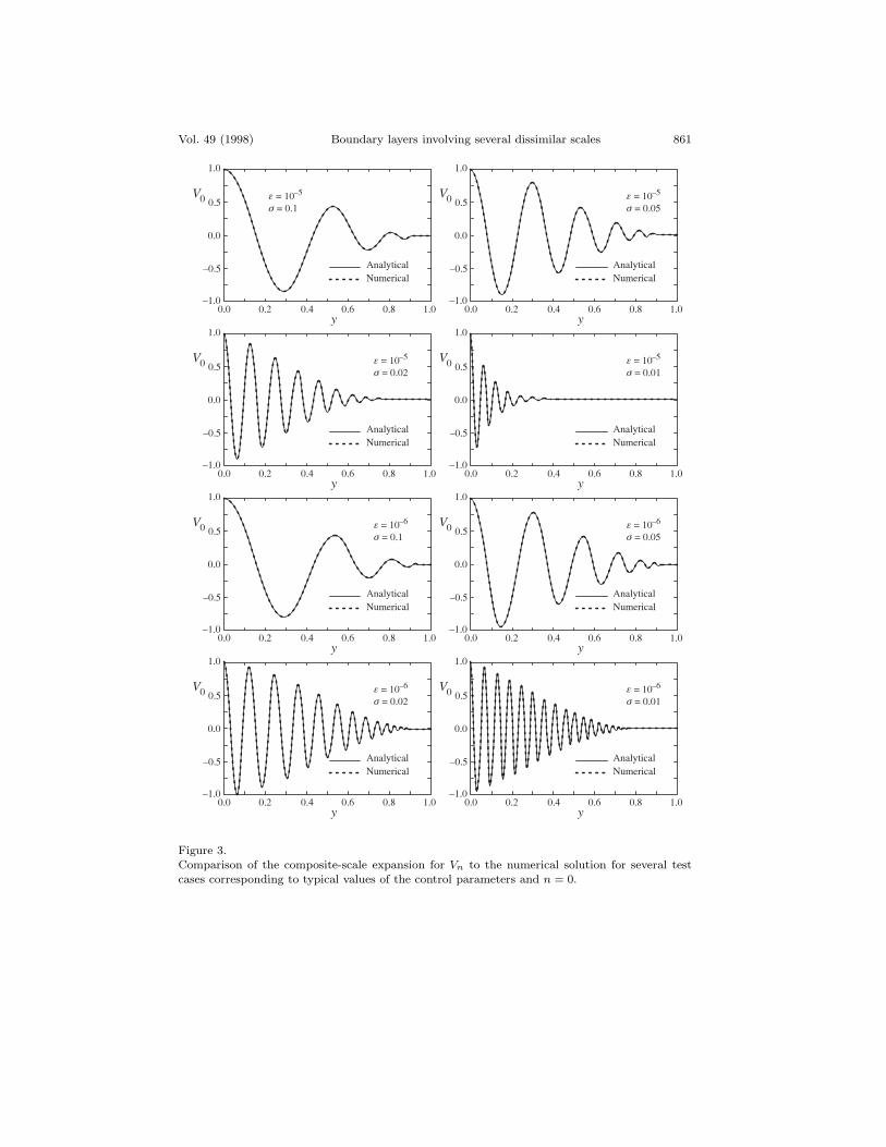
Profiles of Vn(y) corresponding to the composite-scale solution given by (5.22)are shown along with the numerical solution of (2.1) in Figure 3 and Figure 4 wherereal components are compared. In Figure 3, the results are compared at severaltypical values of the controlling parameters, and for the first value of λn. In Figure4, the results are compared for the next four values of λn, and at a typical value ofσ. The striking similarity between numerical and analytical results is reassuringand gets even better at smaller ε.

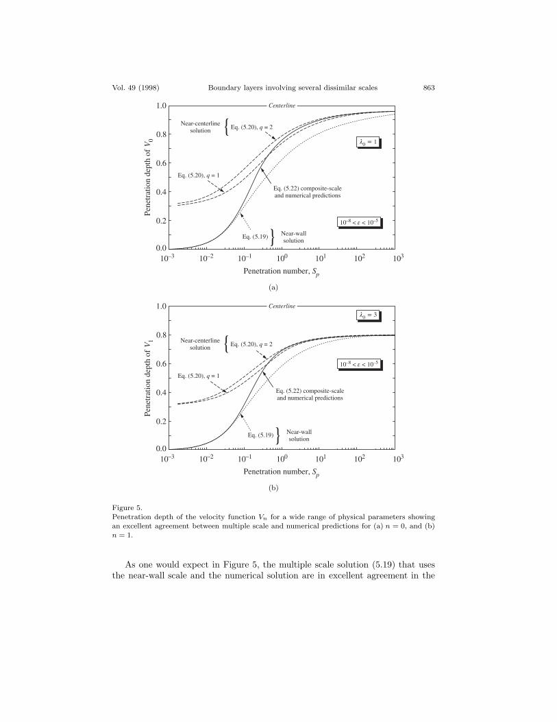
The function Vn(y) is best described as an upward-traveling harmonic wavewith an amplitude which suffers exponential damping with increasing distancefrom the wall. This damping is found to depend primarily on the viscous pa-rameter, ξ; its dependence on σ is found to be insignificant as could be inferredfrom the spatial attenuation term of (5.22). In order to compare numerical andanalytical results in a very wide range of physical parameters, and to provide fur-ther reassurance that the favorable trends depicted in Figures 3-4 are not merelyfortuitous, the 99% based depth of penetration of Vn, a measure of the rotationalregion, is displayed in Figure 5, for the first two values of λn, as obtained fromboth numerical and multiple scale solutions. To that end, the depth of penetrationis plotted, for a wide range of ε, versus the penetration number, Sp ≡ ξ−1, whichhas been ascertained in this and similar studies ([4] and [5]) to be the agent incontrol of the spatial attenuation character of the rotational solution.

It should be pointed out that, despite the fact that (2.1) depends on both ε andσ, the perturbation analysis shows that the decay of rotational waves is controlledby a single nondimensional parameter, Sp, which groups both dynamic similarityparameters appearing in the governing differential equation. This important resultcould not have been foretold without the analytical derivation, since dimensionalanalysis and numerical solutions alone are not capable of revealing its existence.As it turns out, the larger the penetration number, the larger the penetrationdepth will be. Additionally, for small penetration numbers, the penetration depthvaries linearly with the penetration number.

Vol. 49 (1998) Boundary layers involving several dissimilar scales 861

Figure 3.Comparison of the composite-scale expansion for Vn to the numerical solution for several testcases corresponding to typical values of the control parameters and n = 0.

862 J. Majdalani ZAMP

Figure 4.Comparison of the composite-scale expansion for Vn to the numerical solution for several testcases corresponding to n = 1, 2, 3, 4, and σ = 0.02, corresponding to a typical value of theStrouhal number of 50.

Vol. 49 (1998) Boundary layers involving several dissimilar scales 863

0.0

10–3 10–2 10–1 100 101 102 103

0.2

0.4

0.6

0.8

1.0

Near-wallsolution

Near-centerlinesolution

Eq. (5.22) composite-scaleand numerical predictions

Pen

etra

tion

dep

thof

V0

Penetration number, Sp

Eq. (5.20), = 2q

Eq. (5.20), = 1q

Eq. (5.19)

10 < < 10–8 –5e

l =0

1

{

{

Centerline

(a)

0.0

10–3 10–2 10–1 100 101 102 103

0.2

0.4

0.6

0.8

1.0

Near-wallsolution

Near-centerlinesolution

Eq. (5.22) composite-scaleand numerical predictions

Pen

etra

tion

dep

thof

V1

Penetration number, Sp

Eq. (5.20), = 2q

Eq. (5.20), = 1q

Eq. (5.19)

10 < < 10–8 –5e

l = 30

{

{

Centerline

(b)

Figure 5.Penetration depth of the velocity function Vn for a wide range of physical parameters showingan excellent agreement between multiple scale and numerical predictions for (a) n = 0, and (b)n = 1.

As one would expect in Figure 5, the multiple scale solution (5.19) that usesthe near-wall scale and the numerical solution are in excellent agreement in the

864 J. Majdalani ZAMP

0.0

10–3 10–2 10–1 100 101 102 103

0.2

0.4

0.6

0.8

1.0

Pen

etra

tion

dep

thof

Vn

Penetration number, Sp

10 < < 10–8 –5e

Centerline

ln = 1

3

5

79

1113

15

Figure 6.Comparison of numerical and analytical predictions of the penetration depth of Vn for a widerange control parameters encompassing realistic physical settings and at several values of λn,n = 0, 1, . . . , 7.

vicinity of the wall. Similarly, the centerline solutions (5.20) are in agreementwith the numerical solution in their applicable domains, forming an envelope ofundetermined size, as predicted by the scaling analysis of section 3. Note thatthe multiple scale solution (5.22) that uses the composite scale and the numer-ical solution concur in the entire domain and for a very wide range of physicalparameters.

This close agreement between numerical and composite-scale predictions is fur-ther demonstrated in Figure 6 where the same trend is shown to persist at highervalues of λn. Note that, for λn > 15 (not shown), the computational results beginto degenerate at high penetration numbers corresponding to invisicid or frictionlessflows. The analytical results, however, remain unaffected.

Finally, it should be mentioned that, by contrast to traditional boundary lay-ers, no single ”inner” boundary-layer region could be located here, to which willcorrespond a unique ”outer” region. This fact offers a plausible explanation for thereason behind the failure of matched asymptotic expansions. Furthermore, andcontrary to conventional boundary layers, the depth of penetration diminishes withincreasing viscosity.

7. Order Verification

In order to determine the order of the error associated with the composite-scale

Vol. 49 (1998) Boundary layers involving several dissimilar scales 865

expansion of Vn given by (5.22), and in order to show that the error tends to zero atthe correct rate as ε→ 0, a simple yet powerful technique described by Bosley [1]will be invoked. Being ideally suited for both complicated and novel perturbationresults, this technique is capable of verifying rigorously the quantitative accuracyof asymptotic expansions and ascertaining the order of accuracy, to ensure thatno mistakes were made during the derivation process. Accordingly, if the error Enassociated with (5.22) could be represented by

En = Kεα (7.1)

then α, representing the order of the error, could be approximated by the slope ofthe linear least-squares fit of the data generated by graphing log(En) versus log(ε)over a range of ε that is devoid of computational instabilities. In accordance withBosley’s technique, the calculated error En can be chosen, for the case at hand,to be the maximum absolute error over the domain of interest between analyticaland accurate numerical results. For that purpose we define

En = maxy∈[0,1]σ=const

∣∣Vnumerical(y, n, σ, ε)− Vanalytical(y, n, σ, ε)∣∣ (7.2)

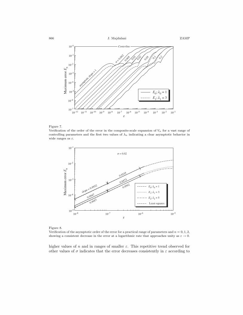
where the analytical component is calculated from (5.22) and the numerical com-ponent from solving (2.1) over the interval [0, 1] by use of a classical fourth-orderRunge-Kutta scheme and a variable mesh size ranging from 10−6 to 10−9. Themaximum error defined by (7.2) is plotted versus ε, which is very finely spacedon the interval shown, in Figure 7, for a vast range of controlling parameters andn = 0, 1. Fitting linear least-squares to the data indicates that the order of theerror approaches unity very rapidly as ε→ 0.

What is very interesting to note is that the regions where deviations from lin-earity are observed correspond to improbable or unrealistic physical settings, andto settings where the mathematical model used to approximate reality deteriorates.For instance, when σ = 0.2, the rate of decrease in the error starts fluctuating whilemaintaining the same overall asymptotic order. This can be attributed to the factthat σ = 0.2 corresponds to a quasi-steady field for which the mathematical model,intended for oscillatory fields, begins degenerating. Additionally, for large ε alonglines of constant σ, the asymptotic rate of the error cannot be observed as clearly.This can be attributed to the fact that ε = vω−1h−2 cannot exceed certain limitsby virtue of physical restrictions imposed on viscosity, frequency, and height of achannel.

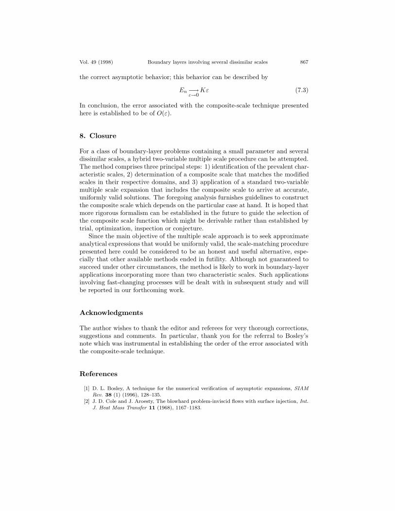
A closer look at the asymptotic behavior of the error is given in Figure 8 fora typical value of σ, and a practical range of ε, for n = 0, 1, 2. The linear slopesobtained from least-squares are provided for two distinct ranges of ε with a highcorrelation coefficient of 1.0000. The results from least-squares are shown by thinsolid lines, and the ranges corresponding to ε ∈ [10−7, 10−6] and ε ∈ [10−8, 10−7]are indicated by parentheses. Clearly, the slope approaches unity more rapidly at

866 J. Majdalani ZAMP

Figure 7.Verification of the order of the error in the composite-scale expansion of Vn for a vast range ofcontrolling parameters and the first two values of λn indicating a clear asymptotic behavior inwide ranges os ε.

Figure 8.Verification of the asymptotic order of the error for a practical range of parameters and n = 0, 1, 2,showing a consistent decrease in the error at a logarithmic rate that approaches unity as ε→ 0.

higher values of n and in ranges of smaller ε. This repetitive trend observed forother values of σ indicates that the error decreases consistently in ε according to

Vol. 49 (1998) Boundary layers involving several dissimilar scales 867

the correct asymptotic behavior; this behavior can be described by

En−→ε→0

Kε (7.3)

In conclusion, the error associated with the composite-scale technique presentedhere is established to be of O(ε).

8. Closure

For a class of boundary-layer problems containing a small parameter and severaldissimilar scales, a hybrid two-variable multiple scale procedure can be attempted.The method comprises three principal steps: 1) identification of the prevalent char-acteristic scales, 2) determination of a composite scale that matches the modifiedscales in their respective domains, and 3) application of a standard two-variablemultiple scale expansion that includes the composite scale to arrive at accurate,uniformly valid solutions. The foregoing analysis furnishes guidelines to constructthe composite scale which depends on the particular case at hand. It is hoped thatmore rigorous formalism can be established in the future to guide the selection ofthe composite scale function which might be derivable rather than established bytrial, optimization, inspection or conjecture.

Since the main objective of the multiple scale approach is to seek approximateanalytical expressions that would be uniformly valid, the scale-matching procedurepresented here could be considered to be an honest and useful alternative, espe-cially that other available methods ended in futility. Although not guaranteed tosucceed under other circumstances, the method is likely to work in boundary-layerapplications incorporating more than two characteristic scales. Such applicationsinvolving fast-changing processes will be dealt with in subsequent study and willbe reported in our forthcoming work.

Acknowledgments

The author wishes to thank the editor and referees for very thorough corrections,suggestions and comments. In particular, thank you for the referral to Bosley’snote which was instrumental in establishing the order of the error associated withthe composite-scale technique.

References

[1] D. L. Bosley, A technique for the numerical verification of asymptotic expansions, SIAMRev. 38 (1) (1996), 128–135.

[2] J. D. Cole and J. Aroesty, The blowhard problem-inviscid flows with surface injection, Int.J. Heat Mass Transfer 11 (1968), 1167–1183.

868 J. Majdalani ZAMP

[3] J. Kevorkian and J. D. Cole, Multiple Scale and Singular Perturbation Methods, Springer-Verlag, New York 1996.

[4] J. Majdalani, Improved flowfield models in rocket motors and the Stokes layer with sidewallinjection, Ph. D. dissertation, University of Utah (1995).

[5] J. Majdalani and W. K. Van Moorhem, A multiple-scales solution to the acoustic boundarylayer in solid rocket motors, J. Propulsion Power (JPP) 13 (2) (1997), 186–193.

[6] J. Murdock, Perturbations: Theory and Methods, Wiley, New York 1991.[7] J. Murdock, Validity of the multiple scale method for very long intervals, J. Appl. Math.

Phys. (ZAMP) 47 (1996), 760–789.[8] D. C. Wilcox, Perturbation Methods in the Computer Age, DCW Industries, Inc., La

Canada, CA 1995.

Joseph MajdalaniDepartment of Mechanical and Industrial EngineeringMarquette UniversityMilwaukee WI 53233, USA(e-mail: maji@marquette.edu)

(Received: June 17, 1997; revised: October 21, 1997)