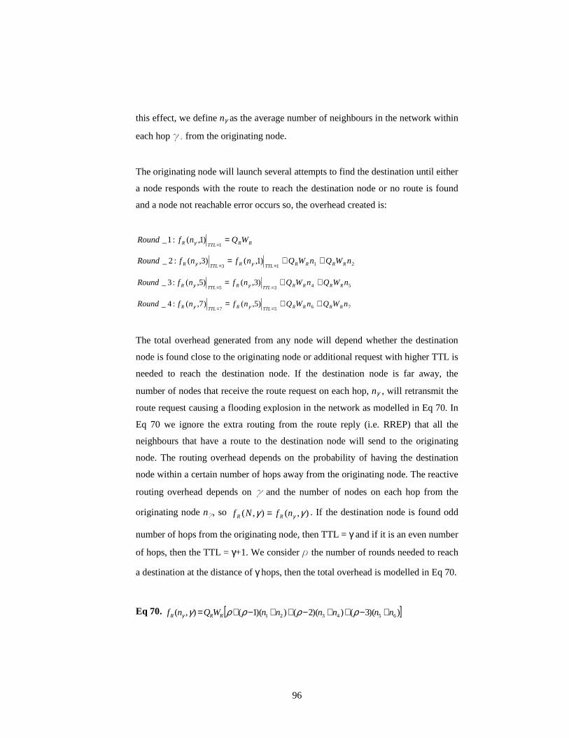
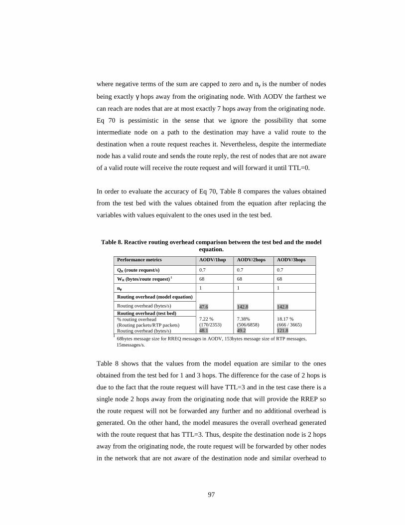
Helsinki University of Technology, Networking Laboratory Teknillinen Korkeakoulu, Tieteverkkolaboratorio Espoo 2007 Report 4/2007 A Hybrid Routing Approach for Ad hoc Networks Jose Costa-Requena Dissertation for the degree of Doctor of Science in Technology to be presented with due permission of the Department of Electrical and Communications Engineering, for public examination and debate in Auditorium S1 at Helsinki University of Technology (Espoo, Finland) on the 7 th of December, 2007, at 12 noon. Helsinki University of Technology Department of Electrical and Communications Engineering Networking Laboratory Teknillinen Korkeakoulu Sahko- ja Tietoliikennetekniikan Osasto Tietoverkkolaboratorio
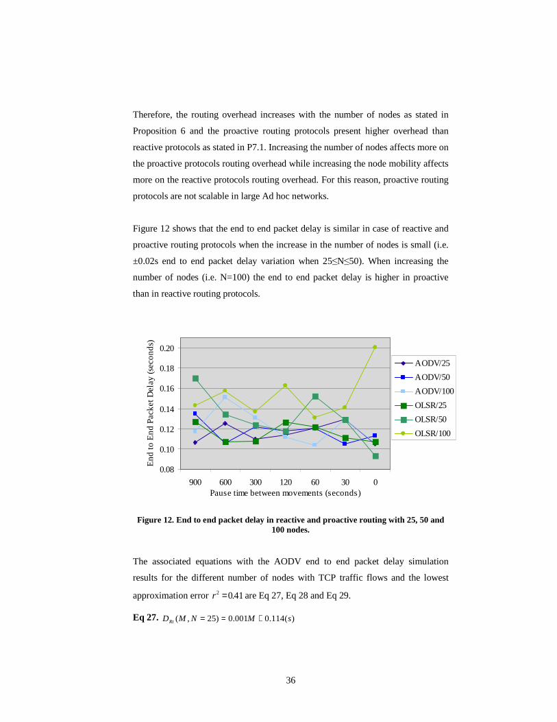
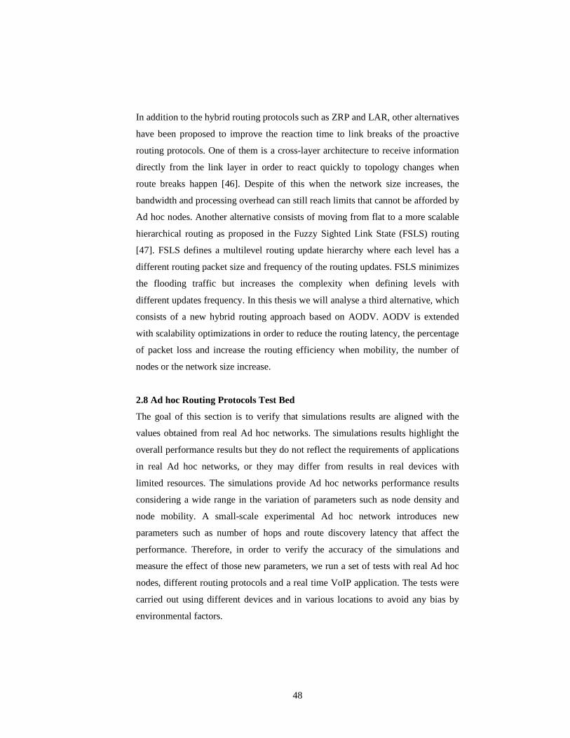
Transcript
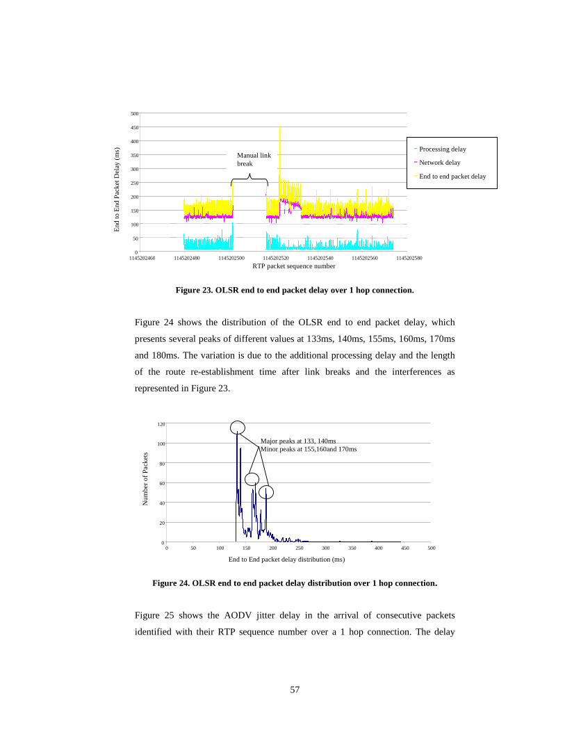
Helsinki University of Technology, Networking Laboratory
Teknillinen Korkeakoulu, Tieteverkkolaboratorio
Espoo 2007 Report 4/2007
A Hybrid Routing Approach for Ad hoc
Networks
Jose Costa-Requena
Dissertation for the degree of Doctor of Science in Technology to be presented with due permission of the Department of Electrical and Communications Engineering, for public examination and debate in Auditorium S1 at Helsinki University of Technology (Espoo, Finland) on the 7th of December, 2007, at 12 noon.
Helsinki University of Technology Department of Electrical and Communications Engineering Networking Laboratory Teknillinen Korkeakoulu Sahko- ja Tietoliikennetekniikan Osasto Tietoverkkolaboratorio
II
Distribution: Helsinki University of Technology Networking Laboratory P.O. Box 3000 FIN-02015 TKK Finland Tel. +358 9 451 2461 Fax. +358 9 451 2474 ISBN 978-951-22-8910-3 ISSN 1458-0322 Otamedia Oy Espoo 2007
ABSTRACT OF DOCTORAL DISSERTATION HELSINKI UNIVERSI TY OF TECHNOLOGY P.O.BOX 1000, FIN-02015 HUT http://www.hut.fi/
Author Lic. Jose Costa-Requena
Name of the dissertation A Hybrid Routing Approach for Ad hoc Networks
Monograph Article dissertation (summary + original articles)
Department Department of Electrical and Communications Engineering Laboratory Networking Laboratory Field of Research Networking, Ad hoc networks Opponent(s) Professor Pietro Michiardi (Eurecom) Pre-examiners Professor Timo Hamäläinen (University of Jyväskylä) and Professor Carlos Pomalaza-Raez (Indiana-Purdue University) Supervisor Professor Raimo Kantola (Helsinki University of Technology)
Abstract
Ad hoc networking is a technology still under development and there are several proposals for defining the most suitable routing protocol. No single routing protocol proposed so far performs optimally under the kind of dynamic conditions possible in Ad hoc networks.
We analyse the performance of existing Ad hoc routing protocols using simulations and a test bed. Based on the results, the goal of this thesis is to design a hybrid routing approach for Ad hoc networks that we name Scalable Ad hoc Routing Protocol (SARP). A novel routing algorithm that responds to the drawbacks of existing routing protocols is analysed and implemented. However, rather than proposing another protocol, this study extends the well-known routing protocol, Ad hoc On Demand Distance Vector (AODV), with a new broadcast algorithm to accommodate the new routing design.
The contribution of the nodes to the routing functionality is critical for establishing Ad hoc networks. We analyse the incentives to participate in the routing functions using game theory. The Scalable Ad hoc Routing Protocol defines a novel architecture that integrates with the routing protocol a rewarding mechanism for the participating nodes. This architecture facilitates the cooperation of the nodes in the Ad hoc networks routing functionality.
Keywords Ad hoc networking, routing, QoS measurements, game theory.
ISBN (printed) 978-951-22-8910-3 ISSN (printed) 1458-0322
ISBN (pdf) 978-951-22-8911-0 ISSN (pdf) 1458-0322
Language English Number of Pages 157
Publisher Networking Laboratory / Helsinki University of Technology
Print distribution
The dissertation can be read at http://lib.tkk.fi/Diss/2007/isbn9789512289110/
Vaitöskirjan nimi Hybridireititysmenetelemä Ad hoc Verkkoja varten
Käsikirjoituksen päivämäärä 20.8.2007 Korjatun käsikirjoituksen 20.11.2007
Väitöstilaisuuden ajankohta 7.12.2007
Monografia Yhdistelmäväitöskirja (yhteenveto ja erillisartikkelit)
Osasto Sähkö- ja tietoliikenntekniikan osasto Laboratorio Tietoverkkolaboratorio Tutkimusala Adhocverkot Vastaväittäjä Professori Pietro Michiardi (Eurecom) Esitarkastajat Professori Timo Hamäläinen (University of Jyväskylä) ja Professori Carlos Pomalaza-Raez (Indiana-Purdue University) Työn valvoja Professori Raimo Kantola (Teknillinen Korkeakoulu)
Tiivistelmä
Ad hoc verkot on vielä kehityksen alla oleva teknologia ja tarkoitukseen sopivia reititysprotokollia on ehdotettu useita. Yksikään tähän asti ehdotettu reititysprotokolla ei toimi optimaalisesti ad hoc verkkojen mahdollisesti muuttuvissa olosuhteissa.
Työssä analysoidaan olemassa olevia ad hoc reititysprotokollia simuloinnin ja koeympäristön avulla. Näiden tulosten perusteella tämän tutkimuksen tavoitteena on suunnitella reititysmenetelmä, jota kutsutaan skaalautuvaksi ad hoc reititysprotokollaksi (SARP, Scalable Ad hoc Routing Protocol). Työssä analysoidaan ja toteutetaan uudenlainen reititysalgoritmi, joka ratkaisee nykyisten protokollien ongelmia. Työssä ei kuitenkaan ehdoteta kokonaan uutta reititysprotokollaa, vaan uusi reititysmenetelmä toteutetaan laajentamalla AODV (Ad hoc On Demand Distance Vector)-reititysprotokollaa uudella yleislähetysmekanismilla.
Solmujen osallistuminen reititystoimintaan on ad hoc verkkojen muodostumisessa tärkeää. Analysoimme halukkuutta osallistua reititystoimintoihin peliteo rian avulla. SARP -protokolla määrittelee uuden arkkitehtuurin, joka sisältää osallistuvia solmuja palkitsevan mekanismin. Tämä arkkitehtuuri tukee solmujen yhteistyötä reititystoiminnassa.
Asiasanat Ad hoc verkot, reititysprotokolla, QoS liikennemittaukset, game theory.
UDC Sivumäärä 157
ISBN (painettu)… 978-951-22-8910-3 ISBN (pdf) 978-951-22-8911-0
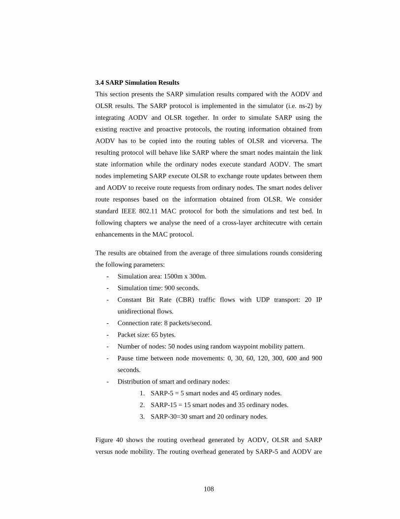
1.4 Structure of the Thesis .................................................................................... 6
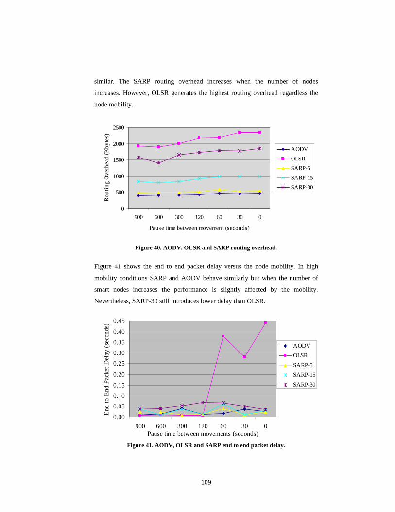
Ad hoc Routing Protocols Analysis ....................................................................... 7
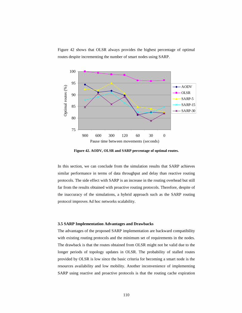
2.1 Addressing and Reachability .......................................................................... 7
2.2 Reactive Ad hoc Routing Protocols .............................................................. 11
2.3 Proactive Ad hoc Routing Protocols............................................................. 13
2.4 Hybrid Ad hoc Routing Protocols................................................................. 13
2.5 Ad hoc Routing Protocols Evaluation........................................................... 14
2.6 Proactive versus Reactive Simulation Comparison ...................................... 20 2.6.1 Simulation Results on Mobility ............................................................. 22 2.6.2 Simulation Results on Scalability .......................................................... 32 2.6.3 Complexity in Reactive and Proactive Routing Protocols..................... 44
2.7 Ad hoc Routing Protocols Simulation Conclusions ...................................... 44
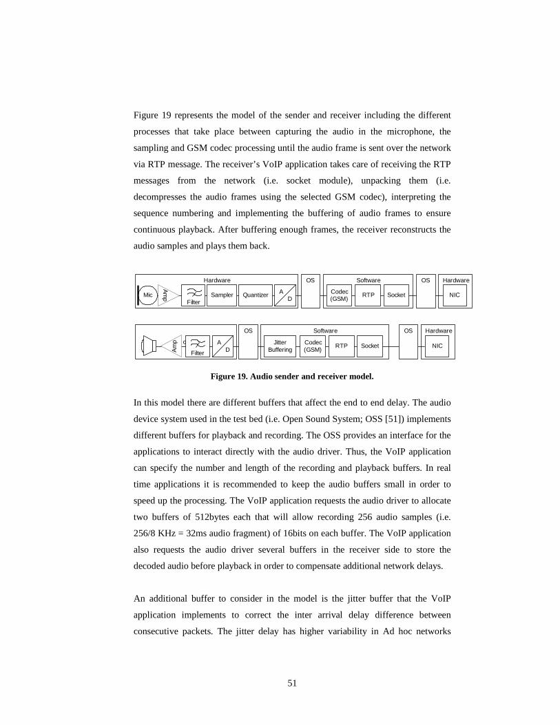
2.8 Ad hoc Routing Protocols Test Bed .............................................................. 48 2.8.1 Testing a Real Time Voice over IP Application.................................... 49 2.8.2 Test Bed Results Conclusions................................................................ 68
2.9 Ad hoc Routing Requirements....................................................................... 70
Performance Modelling of the Hybrid Routing Approach ............................... 78
3.1 Performance Metrics in Fixed Networks ...................................................... 79
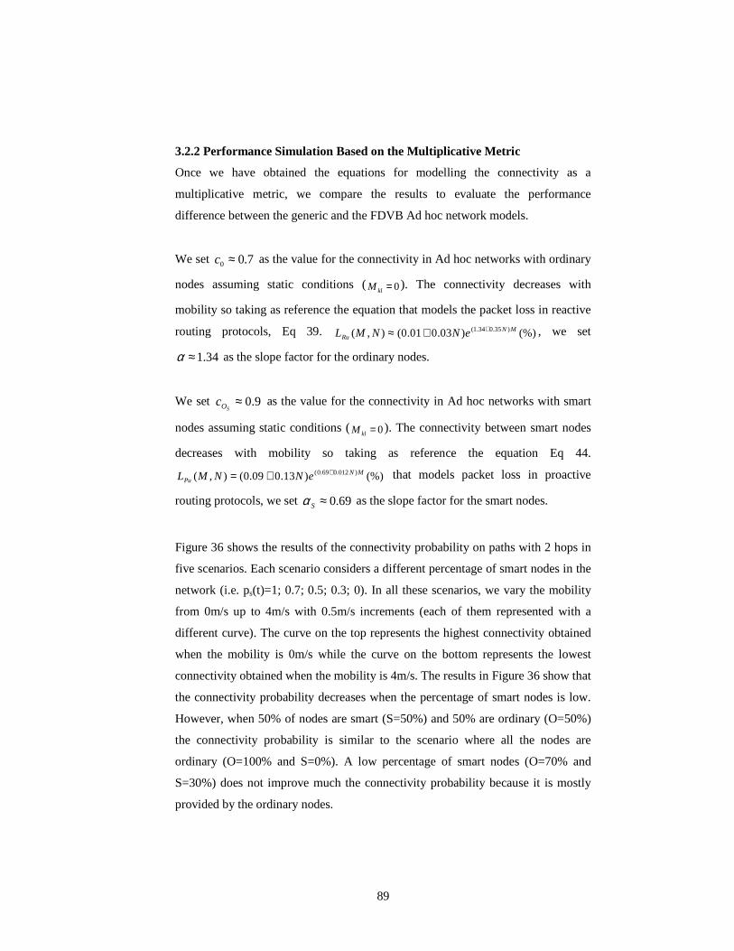
3.2 Performance Metrics in Ad hoc Networks .................................................... 81 3.2.1 Multiplicative Metric of the Ad hoc Networks Model .......................... 85 3.2.2 Performance Simulation Based on the Multiplicative Metric................ 89 3.2.3 Concave Metric of the Ad hoc Network Model..................................... 91 3.2.4 Performance Simulations Based on the Concave Metric....................... 99 3.2.5 Additive Metric of the Ad hoc Network Model................................... 102 3.2.7 Ad hoc Model Evaluation Conclusions ............................................... 103
TKK Teknillinen Korkeakoulu (Helsinki University of Technology)
TTL Time To Live
UDP User Datagram Protocol
VoIP Voice over IP
WLAN Wireless Local Area Networks
ZRP Zone Routing Protocol
vii
List of Tables
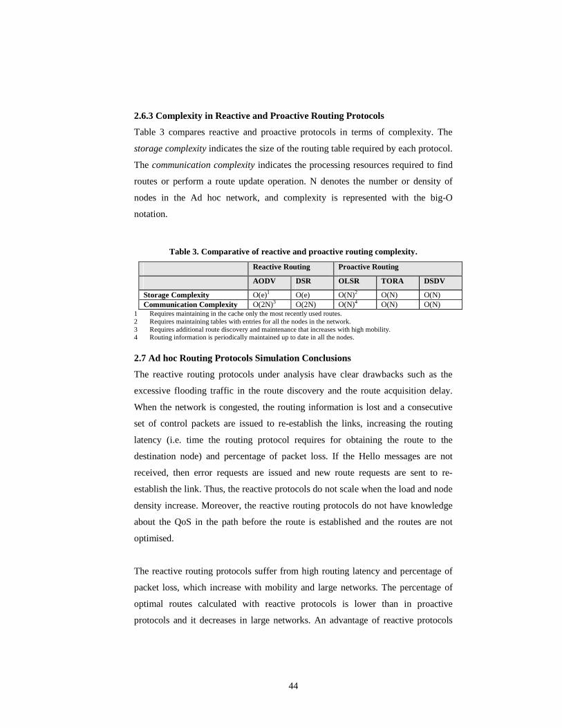
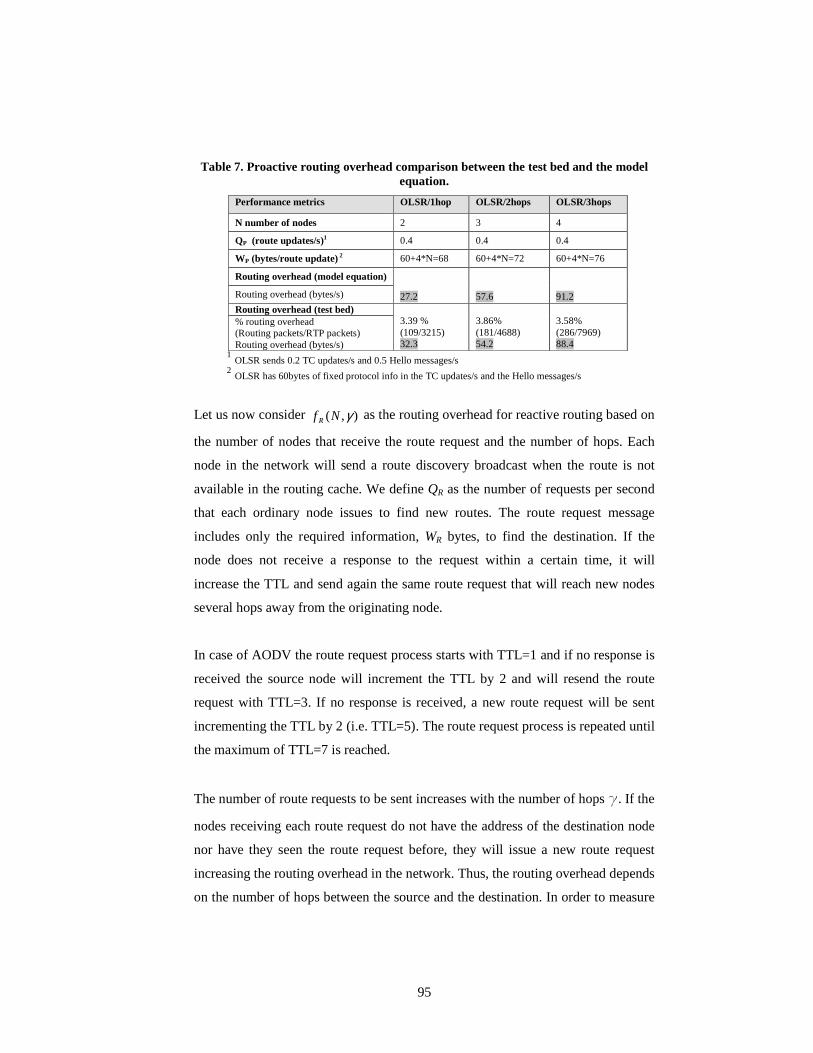
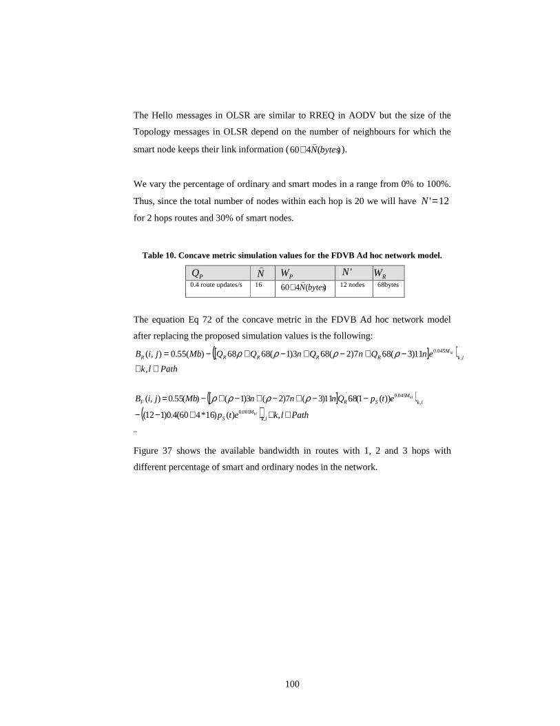
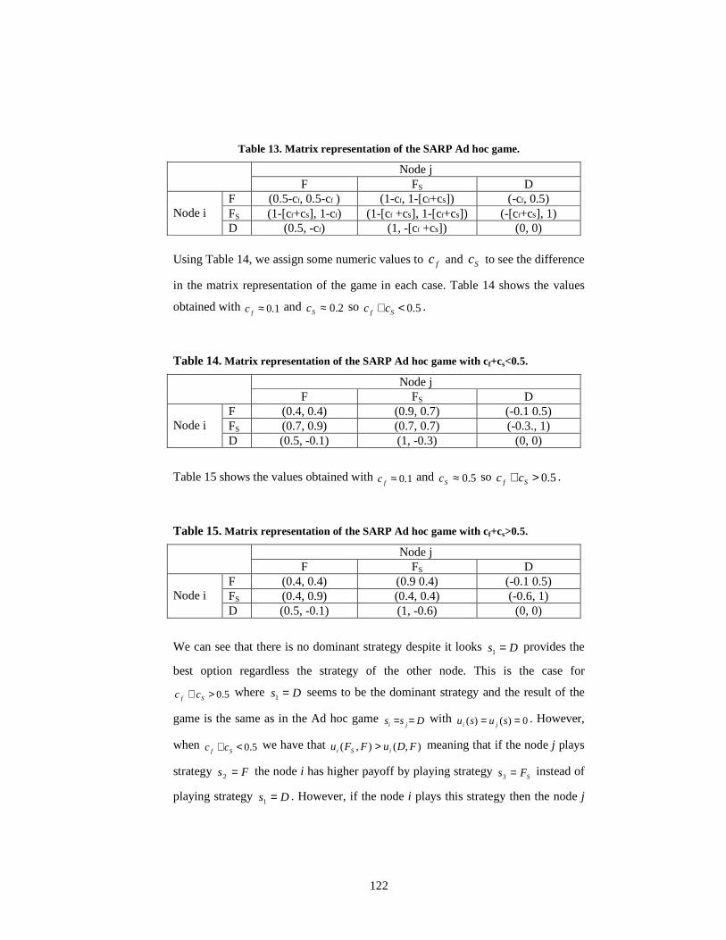
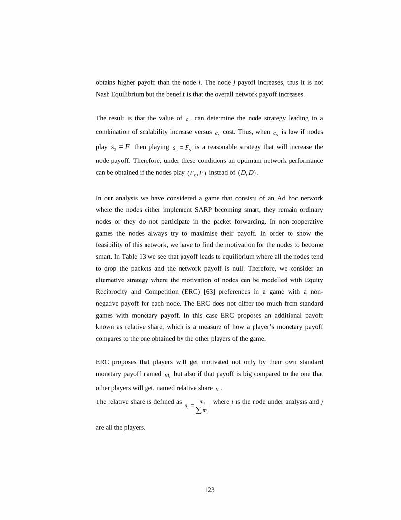
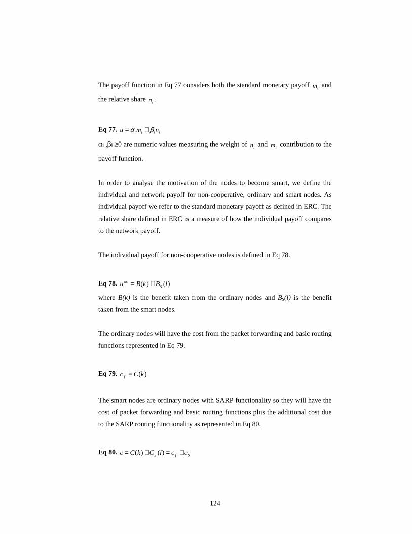
Table 1. System variables. ................................................................................................... 14 Table 2. Performance metrics. ............................................................................................. 14 Table 3. Comparative of reactive and proactive routing complexity. .................................. 44 Table 4. Summary of performance metrics for AODV and OLSR over 1, 2 and 3 hop connections. ......................................................................................................................... 60 Table 5. Ad hoc network model basic variables. ................................................................. 81 Table 6. Ad hoc network model metrics.............................................................................. 85 Table 7. Proactive routing overhead comparison between the test bed and the model equation. .............................................................................................................................. 95 Table 8. Reactive routing overhead comparison between the test bed and the model equation. .............................................................................................................................. 97 Table 9. Concave metric simulation values for the generic Ad hoc network model. .......... 99 Table 10. Concave metric simulation values for the FDVB Ad hoc network model......... 100 Table 11. Matrix representation of the prisoner’s dilemma game. .................................... 115 Table 12. Matrix representation of the basic Ad hoc network game. ................................ 117 Table 13. Matrix representation of the SARP Ad hoc game. ............................................ 122 Table 14. Matrix representation of the SARP Ad hoc game with cf+cs<0.5...................... 122 Table 15. Matrix representation of the SARP Ad hoc game with cf+cs>0.5...................... 122
viii
List of Figures
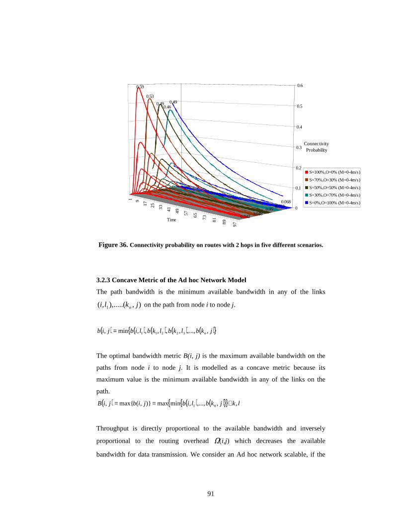
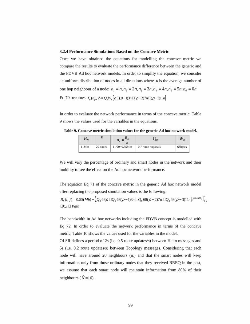
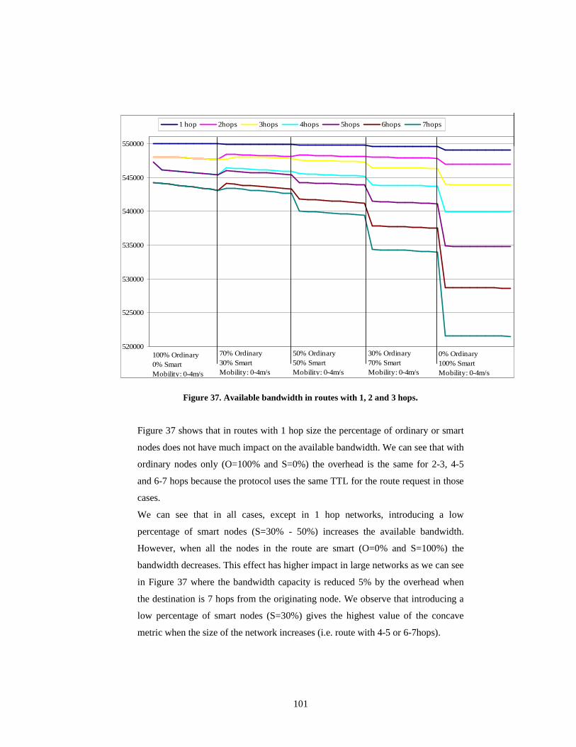
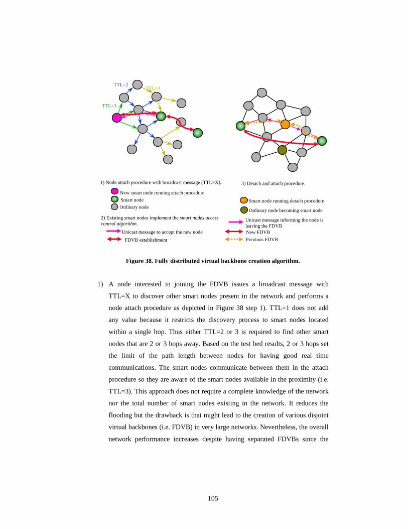
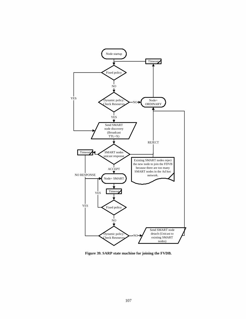
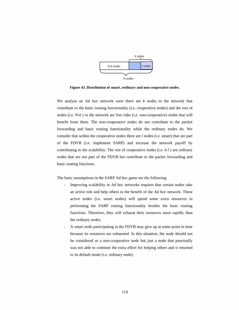
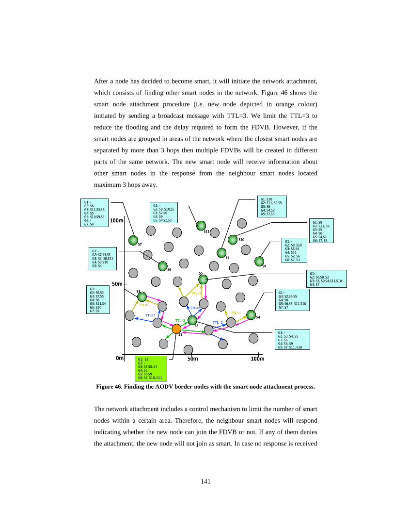
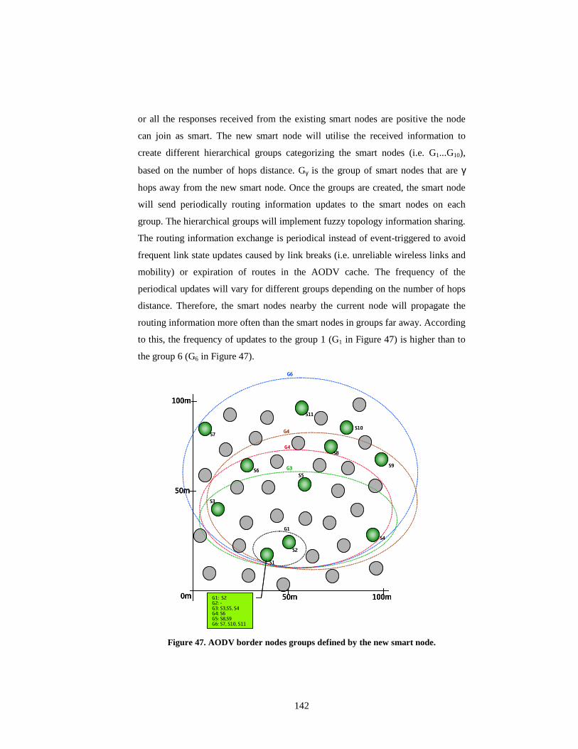
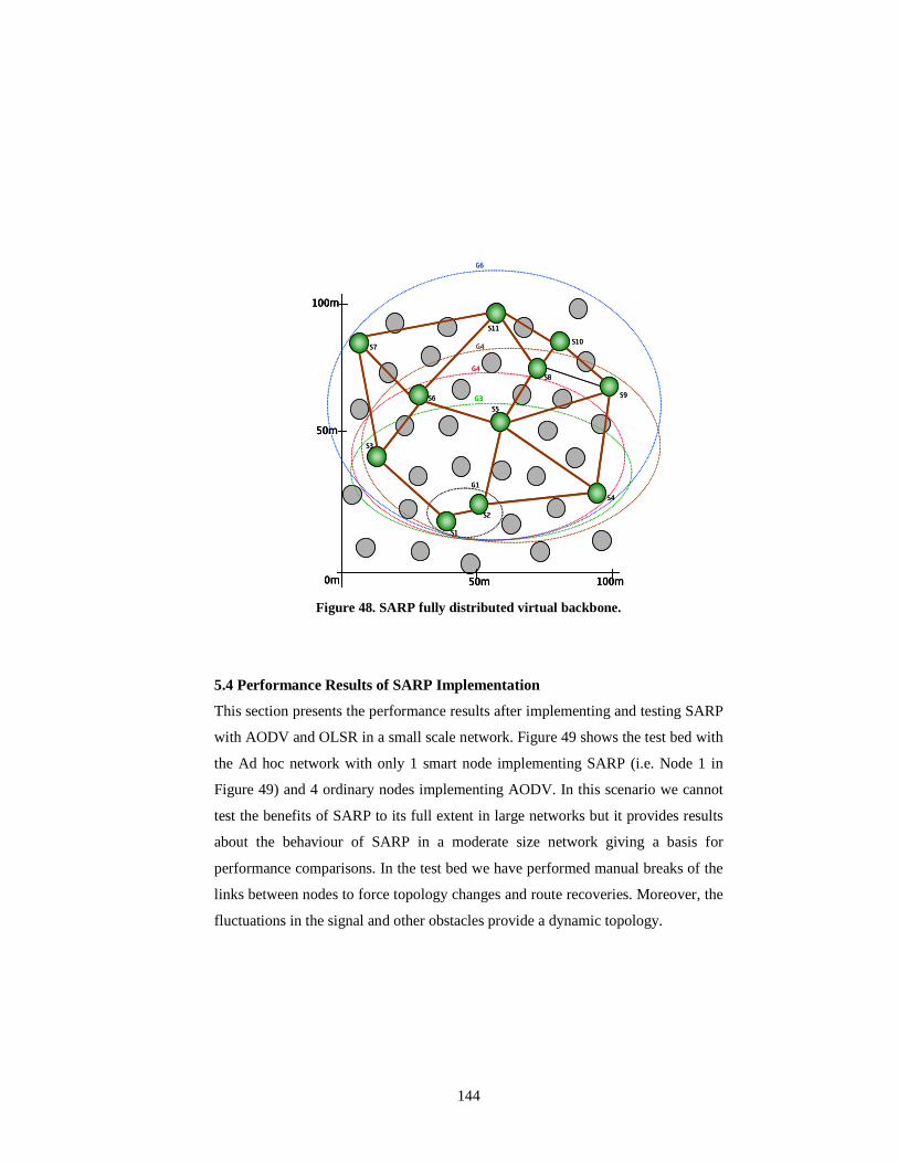
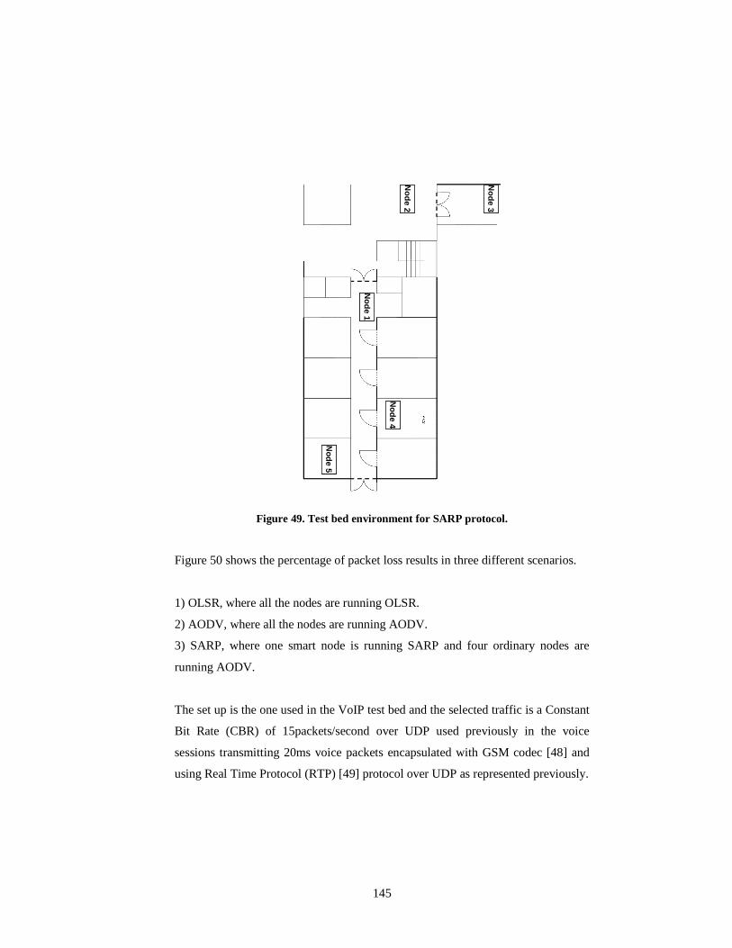
Figure 1. Routing protocols between autonomous systems. .................................................. 9 Figure 2. Cluster-based network routing. ............................................................................ 10 Figure 3. Routing overhead versus node mobility. .............................................................. 23 Figure 4. Routing overhead versus node mobility and transport protocol. .......................... 24 Figure 5. End to end packet delay versus node mobility. .................................................... 25 Figure 6. End to end packet delay versus node mobility and transport protocol. ................ 27 Figure 7. Percentage of packet loss versus node mobility. .................................................. 28 Figure 8. Percentage of packet loss versus node mobility and transport protocol. .............. 29 Figure 9. Percentage of optimal routes versus node mobility.............................................. 30 Figure 10. Percentage of optimal routes versus node mobility and transport protocol........ 31 Figure 11. Routing overhead in reactive and proactive routing with 25, 50 and 100 nodes.33 Figure 12. End to end packet delay in reactive and proactive routing with 25, 50 and 100 nodes.................................................................................................................................... 36 Figure 13. Percentage of packet loss in reactive and proactive routing with 25, 50 and 100 nodes.................................................................................................................................... 39 Figure 14. Percentage of optimal routes in proactive and reactive routing with 25, 50 and 100 nodes............................................................................................................................. 41 Figure 15. Throughput versus mobility in reactive, proactive and hybrid routing. ............. 47 Figure 16. Routing overhead versus mobility in reactive, proactive and hybrid routing..... 47 Figure 17. Ad hoc routing framework. ................................................................................ 49 Figure 18. VoIP packet structure. ........................................................................................ 50 Figure 19. Audio sender and receiver model. ...................................................................... 51 Figure 20. VoIP test bed scenarios. ..................................................................................... 55 Figure 21. OLSR jitter delay over 1 hop connection........................................................... 56 Figure 22. Distribution of the OLSR jitter delay over 1 hop connection............................. 56 Figure 23. OLSR end to end packet delay over 1 hop connection....................................... 57 Figure 24. OLSR end to end packet delay distribution over 1 hop connection. .................. 57 Figure 25. AODV jitter delay over 1 hop connection.......................................................... 58 Figure 26. Distribution of the AODV jitter delay over 1 hop connection. .......................... 58 Figure 27. AODV end to end packet delay over 1 hop connection. .................................... 59 Figure 28. AODV end to end packet delay distribution over 1 hop connection. ................. 59 Figure 29. AODV and OLSR routing overhead over 1, 2 and 3 hop connections............... 66 Figure 30. AODV and OLSR routing latency over 1, 2 and 3 hop connections.................. 68 Figure 31. Small versus large networks routing requirements............................................. 71 Figure 32. Node classification based on contribution to network topology information..... 73 Figure 33. Fully distributed virtual backbone created with multiple cluster heads. ............ 76 Figure 34. Consumed and residual battery capacities in smart and ordinary nodes. ........... 83 Figure 35. Probability of arrival, death and smart nodes left in the Ad hoc network. ......... 84 Figure 36. Connectivity probability on routes with 2 hops in five different scenarios........ 91 Figure 37. Available bandwidth in routes with 1, 2 and 3 hops.........................................101 Figure 38. Fully distributed virtual backbone creation algorithm......................................105 Figure 39. SARP state machine for joining the FVDB...................................................... 107 Figure 40. AODV, OLSR and SARP routing overhead. ................................................... 109 Figure 41. AODV, OLSR and SARP end to end packet delay.......................................... 109 Figure 42. AODV, OLSR and SARP percentage of optimal routes. ................................. 110 Figure 43. Distribution of smart, ordinary and non-cooperative nodes. ............................ 119 Figure 44. SARP logical architecture. ............................................................................... 136 Figure 45. Smart node selection state machine.................................................................. 137 Figure 46. Finding the AODV border nodes with the smart node attachment process...... 141 Figure 47. AODV border nodes groups defined by the new smart node. .......................... 142 Figure 48. SARP fully distributed virtual backbone.......................................................... 144
ix
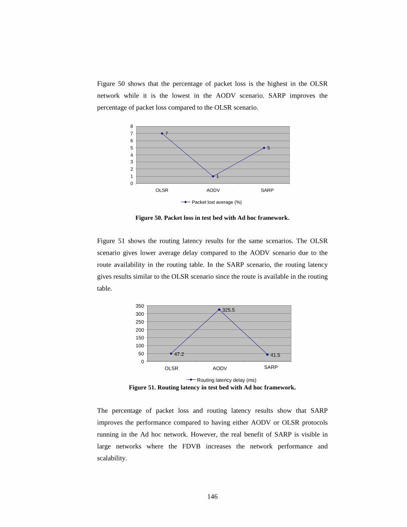
Figure 49. Test bed environment for SARP protocol. ....................................................... 145 Figure 50. Packet loss in test bed with Ad hoc framework................................................ 146 Figure 51. Routing latency in test bed with Ad hoc framework. ....................................... 146
1
Chapter 1
Introduction
Ad hoc networks are envisioned as a key technology for ubiquitous networking. It
is a suitable technology for embedded network devices in multiple environments
such as vehicles, mobile telephones and personal appliances. As an infrastructure-
less technology, it will allow users to create their Personal Area Networks (PAN).
The benefit of Ad hoc networks is that users can create the network automatically
when needed and tear it down if it is not required anymore. The network can be
created at any point in time for any communication purpose such as leisure,
military or disaster situations. Ad hoc networks have an undefined lifetime since
they can be up and running momentarily or permanently as long as there is a group
of users that are willing to be part of the network.
Nowadays, mobile computers and personalized applications are indispensable.
Users demand connectivity at any time at any place, even where the appropriate
infrastructure is not available. In this kind of scenarios, it is necessary that wireless
devices learn how to communicate among themselves without routers, base stations
or service providers. Ad hoc networks could be the solution to fulfil these user
needs but they present new challenges that have not been primary concerns in fixed
networks deployment until now.
1.1 Networking Requirements in Ad hoc Networks
In Ad hoc networks the link state information changes whenever users move and
create interferences to each other. Ad hoc networks are self-established without
2
previous knowledge of the environment. Ad hoc nodes require a set of mechanisms
to allow the devices to be autonomously integrated and configured as part of the
Ad hoc network.
Network scalability is the ability to expand or reduce the number of nodes and size
of the network while maintaining similar performance for each user. Ad hoc nodes
have to perform the routing functionality and maintain the network topology
information, while keeping track of the connection with other nodes. They must
also be able to react fast to network changes and dynamically adapt to the new
topology. Therefore, the overall Ad hoc network performance is affected by the
size of the network, the number of nodes, their mobility and resources.
Ad hoc nodes cannot rely on a fixed server that would inform about the services
available in the Ad hoc network. Therefore, each node needs its own mechanism to
discover the network capabilities and configure itself to the services available in
the Ad hoc network. Besides these, Ad hoc networks have to interconnect with
other IP based technologies such as fixed Wireless Local Area Networks (WLAN)
and 3G networks. For that reason, Ad hoc nodes have to act as routers and
constantly search for the services available in the networks. The nodes that become
part of Ad hoc networks contribute to the overall network performance while
spending their own resources. This leads to a high energy consumption that
exhausts the batteries of the nodes.
1.2 Objectives of the Thesis
In recent years it has been proven that there is no single protocol that
accommodates different conditions in Ad hoc networks [1] [2]. Moreover, not all
the nodes have the same requirements in terms of mobility and resources.
Therefore, it is difficult to design a single protocol that simultaneously meets all
the network variations and the different node requirements.
The objective of this thesis is to design and implement a new hybrid routing
approach named Scalable Ad hoc Routing Protocol (SARP). The main purpose of
3
SARP is to enable Ad hoc networks scalability. This approach has to be able to
meet the demands of the Ad hoc network when it reduces or increases the size and
the number of nodes. Moreover, it has to be suitable for nodes with different
mobility and resource constrains. Test bed results and simulations of existing
routing protocols are used as the basis for SARP design. A mathematical model of
Ad hoc networks is defined to evaluate SARP performance and optimize the
protocol.
A protocol enabling Ad hoc networks scalability requires that some nodes spend
additional resources, which may lead into unfairness. This thesis proposes a new
algorithm assessed using game theory [3] that provides a rewarding mechanism for
the Ad hoc nodes contributing towards network scalability. Besides that, a cross-
layer architecture is designed to implement the rewarding algorithm. With this
approach the Ad hoc nodes obtain a fair added value in return for their contribution
to the routing functionality.
SARP is integrated with the cross-layer architecture for enabling network
scalability and implementing the rewarding mechanism. The analysis of the
existing protocols together with the mathematical model evaluation supported the
selection of the Ad hoc On Demand Distance Vector (AODV [4]) as the basis for
SARP implementation.
1.3 Our Contribution
We have studied the different routing protocols used in Ad hoc networks, and
found that each protocol has different drawbacks and benefits depending on the
network topology. We propose a network model based on the results obtained from
simulations and a test bed.
Our main contribution is the following:
1. We run simulations to evaluate the performance of different Ad hoc
routing protocols. The author in cooperation with other students
4
implemented a test bed with a voice over IP application, and the results
were compared to the ones obtained in the simulations. The outcome of
this work is part of the MobileMAN EU project IST-2001-38113 [5].
2. Based on the results from the simulations and the test bed, we propose a
routing protocol to fix some of the drawbacks of reactive, proactive and
some hybrid routing protocols. Using those results as baseline, we devise a
mathematical model to evaluate the network performance of existing Ad
hoc routing protocols and compare the results with the proposed routing
protocol.
3. We apply game theory [3] to analyse the incentives required to deploy the
proposed routing protocol. Moreover, based on the game analysis, a cross-
layer architecture with a rewarding system is proposed for implementing
the incentives.
The author’s original contributions can be found in this thesis and the following
publications.
The author instructed nine Master Thesis as preliminary work leading to
this thesis. Preliminary results of what will be published in this thesis were
reported in the respective nine Master Thesis and joint conference papers
based on those Master Thesis. In particular, Master Thesis [6] includes
part of the simulation results presented in Chapter 2. Master Thesis [7],
[8], [9], [10], [11] and [12] develop the Ad hoc test bed, and Master Thesis
[13] and [14] provide the test bed performance results partly used in
Chapter 2.
The early simulations and the initial hybrid routing proposal included in
Chapter 2 can be found in [15]. Some of the test bed results in Chapter 2
are published in [16]. The performance metrics model based on the
simulation and test bed results that are used to propose the new fully
distributed virtual backbone (FDVB) algorithm is published in [17]. A
subset of the implementation presented in Chapter 4 including the route
5
cache replication and the original proposal of the FDVB based on smart
nodes is published in [18] and [19]. The architecture proposed in Chapter
4 to implement the FDVB for supporting network scalability can be found
in [20] and [21]. Preliminary work including the network incentives to
implement the proposed hybrid routing protocol is published in [22].
In addition to the publications directly related to Ad hoc networking, the
author previously contributed to Internet addressing, numbering and IN
interoperability routing research. Those are used in this work as
background to analyse scalability in IP networks [23], [24] and [25].
Therefore, part of the content included in several Chapters of this thesis can be
found in existing publications. However, this thesis includes improved versions of
the work presented in those publications. Chapter 2 includes new propositions
obtained from recent simulations. Chapter 3 contains an updated version of the
performance models and simulation results not included in previous publications.
Chapter 4 contributes with new conclusions obtained after reformulating the game
analysis, which are not published in any previous work. The instructed Master
Theses include an early protocol design that has been updated in Chapter 5 with
new algorithms identified after obtaining some preliminary test results from
prototype implementations. Therefore, the work published in the Master Thesis,
conference papers and journals include the preliminary results used as baseline for
this work. Nevertheless, this thesis presents new findings and conclusions
formulated with more detail than in previous publications.
This thesis is structured as a monograph instead of an article dissertation to present
a more coherent and accurate report of the work done by the author and the
students working on this subject. This thesis provides a comprehensive
presentation of the results and a progressive analysis of the subject. Therefore, this
work starts with simulations and a test bed to provide the basic analysis that is
followed by a mathematical model to evaluate the network performance. To
conclude, we introduce a theoretical analysis based on game theory to describe the
6
incentives for implementing the proposed routing protocol and support scalability
in Ad hoc networks.
1.4 Structure of the Thesis
Chapter 2 presents the performance evaluation of existing Ad hoc routing
protocols. The results demonstrate that there is no single protocol suitable for all
the Ad hoc networks. This chapter also highlights the scalability limitations of
some of the existing routing protocols. Based on the performance evaluation we
design a novel hybrid routing approach for Ad hoc networks named Scalable Ad
hoc Routing Protocol (SARP). SARP is specified as a fully distributed virtual
backbone (FDVB) algorithm.
Chapter 3 defines a mathematical model to evaluate SARP performance and
optimize the protocol. The results are used to specify the optimal requirements for
the FDVB algorithm.
Chapter 4 presents the incentives for the nodes to participate in SARP routing
functionality. In this chapter game theory [3] is applied to demonstrate that SARP
requires a cross-layer architecture implementing a rewarding mechanism.
Chapter 5 describes the SARP implementation on top of a reactive routing
protocol, the Ad hoc On demand Distance Vector (AODV) [4]. A novel
architecture based on a cross-layer interaction with the routing protocol is studied.
Chapter 6 presents our conclusions and future work.
7
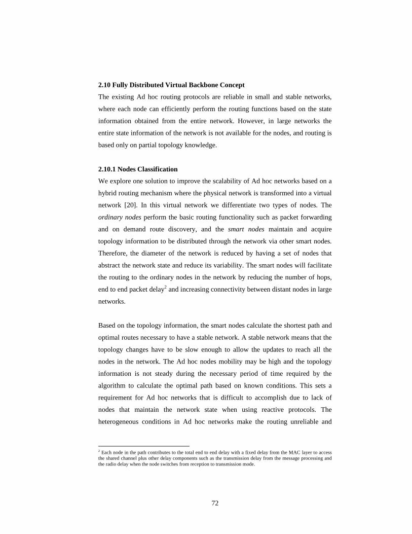
Chapter 2
Ad hoc Routing Protocols Analysis
This chapter introduces a performance evaluation of existing Ad hoc routing
protocols. The performance results presented in this chapter, obtained from
simulations and validated using a test bed, demonstrate that there is no single
protocol suitable for all the Ad hoc networks [26]. This chapter highlights the
performance of reactive, proactive and hybrid routing protocols in terms of
scalability.
2.1 Addressing and Reachability
In Ad hoc networks, the nodes perform the addressing and routing functionalities
making scalability a critical issue in large networks. Before studying the existing
Ad hoc routing protocols and their performance, different addressing approaches
are analysed. As baseline for our study, we briefly review the different solutions
that have been implemented in fixed networks to handle the scalability problems in
addressing.
Addressing is hierarchical (e.g. country code, trunk code and subscriber number) in
existing fixed networks such as Plain Old Telephony Service (POTS) [27] where
each switch maintains a specific numbering block. IP networks addressing was
originally flat [28] but when the number of hosts connected to the network
increased, a mechanism to emulate a hierarchical addressing structure dividing the
addressing space into groups (i.e. address classes A, B, C and D) was established.
The number of nodes kept increasing and the addresses availability was reduced.
8
Therefore, a more flexible hierarchical scheme, the Classless Inter-Domain
Routing (CIDR) [29] was implemented for a more efficient usage of the existing
address space.
Maintaining the names and IP addresses of all the hosts in the network up to date,
required a continuous exchange of messages resulting in network congestion. Thus,
new protocols such as the Dynamic Name Service (DNS) [30], and the Dynamic
Host Configuration Protocol (DHCP) [31] were required.
In Ad hoc networks a similar approach has to be followed due to scalability issues.
Most of the Ad hoc routing protocols have a flat addressing structure where each
node keeps the addresses of the rest of the nodes, similarly to Internet when it was
created. However, as history shows, this approach is not suitable when the number
of nodes in the network is large. The nodes have to store all IP addresses in their
routing tables and they have to maintain the topology information up to date.
Therefore, a hierarchical addressing structure is required for scalable Ad hoc
networks. The drawback is that Ad hoc networks cannot rely on a fixed entity that
assigns the blocks of addresses, making the addressing a significant challenge.
In fixed IP networks moving from flat to hierarchical addressing is feasible because
all the nodes are static and they can easily be grouped under sub networks. The IP
address space remains flat but it is divided into blocks to emulate hierarchical
addressing. Moreover, users want mobility and connectivity with their devices
anywhere. DHCP [31] and Mobile IP [32] are the mechanisms for maintaining the
flat addressing but still allowing the nodes mobility through different sub networks.
DHCP dynamically assigns a new IP address to the nodes accessing the network.
Mobile IP enables nodes to be reachable through different sub networks using their
static IP address. Ad hoc networks could have applied the same mechanisms (i.e.
DHCP or Mobile IP) allowing the nodes to obtain an IP address or maintain their
static IP address when joining the Ad hoc network. However, due to the nature of
Ad hoc networks [33], the availability of DHCP servers or Mobile IP agents cannot
9
be guaranteed. Instead the Ad hoc nodes must acquire the IP addresses on their
own and configure themselves as part of the Ad hoc network.
In fixed networks routers or gateways provide the routing and addressing
functionality and the nodes only store the address of the DNS, DHCP server and
gateway for routing purposes. In principle, fixed networks are made of many
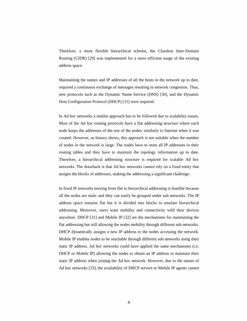
networks (i.e. Autonomous Systems) connected by routers or gateways as depicted
in Figure 1. The routers are nodes that use routing protocols such as Open Shortest
Path First (OSPF) [34] to maintain addressing information and find the routes
between source and destination nodes within the same or different sub networks.
The gateways are routers that maintain addressing information about sub networks
they are bridging using routing protocols such as the Border Gateway Protocol
(BGP) [35].
Figure 1. Routing protocols between autonomous systems.
When a router receives a packet, it checks the destination address looking up the
longest match in the routing table and forwards it to the next router closer to the
destination. If no match for the destination address is found in the router, the packet
will be forwarded to the default route tied to zero in the routing table. The default
Autonomous system AS 2
BGP Router 1
Router 2 Router 3
OSPF
Router 3
Router 2 Router 1
Area 1
Area 2
Area 3
Router 5
Router 6
Router 7
Router 8
Router 9
Router 10
Router 11
Router 12
Router 13
Router 4
Autonomous system AS 1
OSPF
OSPF
OSPF
Autonomous system AS 3
Router 2
Router 1 OSPF
OSPF
BGP BGP
Router 3
10
route address points to the gateway that maintains addressing information of the
other sub networks.
Ad hoc nodes act as routers that cannot rely on any fixed infrastructure devices
such as gateways, DHCP or DNS for addressing assistance. Therefore, Ad hoc
nodes have to include all necessary routing and addressing functionalities
themselves. This means that they must store all routing information and need a
mechanism to discover the routes to other nodes that are outside the local sub
network.
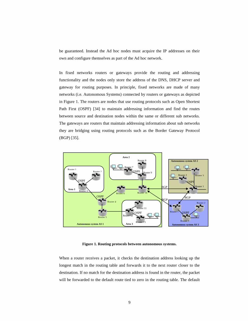
Scalable Ad hoc networks require a hierarchical addressing structure, where the
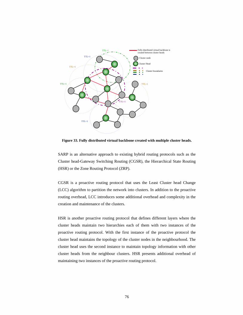
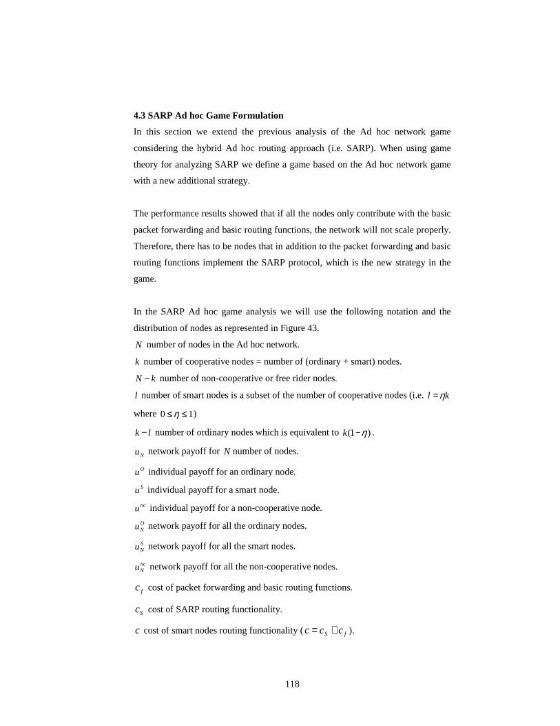
network is partitioned into sub networks or clusters. Figure 2 represents a cluster-
based network with four clusters.
Figure 2. Cluster-based network routing.
A cluster-based network is a network divided into several clusters. Each cluster
consists of a single cluster head and multiple cluster nodes. The cluster head is a
Cluster heads
Cluster nodes
Inter cluster communication
cluster boundaries
Intra cluster communication
Cluster heads
Cluster nodes
Inter cluster communication
cluster boundaries
Intra cluster communication
11
node that performs the routing functionality assigned to gateways in fixed
networks. When a cluster node needs to find a route to a destination node not
located in the same cluster, it will contact the cluster head that acts as a gateway.
The cluster head communicates with other cluster heads in different clusters to find
the route to the destination node.
The communication between nodes in the same cluster is known as intra cluster
communication. Cluster heads establish the inter cluster communication with nodes
outside their own cluster. Cluster heads require additional resources to perform the
gateway functionality. The cluster-based routing decreases the network reliability
because the cluster head may become the bottleneck. Moreover, the algorithm for
selecting the optimal cluster head among the existing cluster nodes is cumbersome.
Nevertheless, from a preliminary analysis on the evolution of the public Internet a
hypothesis can be formulated; a cluster-based routing protocol where the changes
in IP addresses and route updates are localised and do not span the entire
network, is required to guarantee scalability in Ad hoc networks.
The evolution path taken in the fixed Internet to solve the scalability problem
might not be valid for Ad hoc networks and there is no mathematical analysis to
prove that a cluster-based routing protocol is the only solution to make Ad hoc
routing scalable. Therefore, in order to verify this claim, next section describes the
state of the art in some of the existing Ad hoc routing protocols and their
performance. Ad hoc routing protocols can be classified into three categories
reactive, proactive and hybrid [5].
2.2 Reactive Ad hoc Routing Protocols
Reactive Ad hoc routing protocols determine a path on-demand only, meaning that
they search for a single path when a message needs to be delivered. In this section
we briefly describe the Ad hoc On Demand Distance Vector (AODV) [4], the
Dynamic Source Routing (DSR) [36] and the Temporally Ordered Routing
Algorithm (TORA) [37] as the most widely used reactive Ad hoc routing protocols.
12
In AODV the originating node initiates a Route Request (RREQ) message that is
flooded through the network to the destination. The intermediate nodes in the route
record the RREQ message. A Route Reply (RREP) unicast message is sent back to
the originating node as the acknowledgement following the reverse routes
established by the received RREQ message. The intermediate nodes in the route
also record the RREP message in their routing table for future use. Each node
keeps the most recently used route information in its cache. Therefore, AODV is a
simple protocol and does not require excessive resources on the nodes. However,
the routing information available in the nodes is limited, and the route discovery
process may take too much time. The initial RREQ is sent with TTL=1 and if no
RREP is received within a certain time, the TTL is incremented and a new RREQ
is sent. Thus, if the destination node is not close enough, the network is flooded
several times during the RREQ process before a route is found or an error is
notified.
DSR is similar to AODV where RREQ and RREP messages are also used for
discovering the route to the destination. The main difference is that in this case,
these messages also include the entire path information (i.e. addresses of the
intermediate nodes). The drawback is that the route information generates an
overhead that can be excessive when the number of hops or node mobility
increases.
TORA is a reactive routing protocol with some proactive enhancements where a
link between nodes is established creating a Directed Acyclic Graph (DAG) of the
route from the source to the destination. The routing messages are distributed to a
set of nodes following the graph around the changed topology. TORA provides
multiple routes to a destination quickly with minimum overhead. In TORA the
optimal routes are of secondary importance versus the delay and overhead of
discovering new routes.
13
2.3 Proactive Ad hoc Routing Protocols
The proactive protocols are the traditional routing protocols used in fixed IP
networks. These protocols maintain a table with the routing information, and
perform periodic updates to keep it consistent. In this section we will introduce the
Destination Sequenced Distance Vector Routing (DSDV) [38] and the Optimised
Link State Routing (OLSR) [39] as the most representative proactive Ad hoc
routing protocols.
DSDV looks for the optimal path using the Bellman-Ford algorithm [40]. It uses a
full dump or incremental packets to reduce the traffic generated by the routing
updates in the network topology. However, it creates an excessive overhead
because it constantly tries to find the optimal path.
OLSR defines Multipoint Relay (MPR) nodes for exchanging the routing
information periodically. The nodes select the local MPR node that will announce
the routing information to other MPR nodes in the network. The MPR nodes
calculate the routing information for reaching other nodes in the network.
2.4 Hybrid Ad hoc Routing Protocols
This section introduces a hybrid model that combines reactive and proactive
routing protocols but also a location assisted routing protocol.
The Zone Routing Protocol (ZRP) [41] is a hybrid routing protocol that divides the
network into zones. The Intra-Zone Routing Protocol (IZRP) implements the
routing within the zone, while the Inter-zone Routing Protocol (IERP) implements
the routing between zones. ZRP provides a hierarchical architecture where each
node has to maintain additional topological information requiring extra memory.
The Location Aided Routing (LAR) [42] is a location assisted routing protocol that
uses location information for the routing functionality. LAR works similarly to
DSR but it uses location information to limit the area where the route request is
14
flooded. The originating node knows the neighbours location and based on that
selects the closest nodes to the destination as the next hop in the route request.
2.5 Ad hoc Routing Protocols Evaluation
We have described different routing protocols and based on the basic
characteristics of reactive and proactive routing protocols we can formulate a set of
propositions. The propositions will consider the impact of system variables such as
used routing protocol type, node mobility and number of nodes (i.e. node density)
on performance measures such as routing overhead, percentage of packet loss, end
to end packet delay and percentage of optimal routes. At this stage we are not able
to indicate whether there is a linear or polynomial relationship between the system
variables and the performance measures.
AODV, DSR and OLSR, TBRF are the experimental protocols standardized in the
IETF as reactive and proactive routing protocols. The routing protocols under
consideration in this evaluation are AODV and OLSR as the most representative of
reactive and proactive categories.
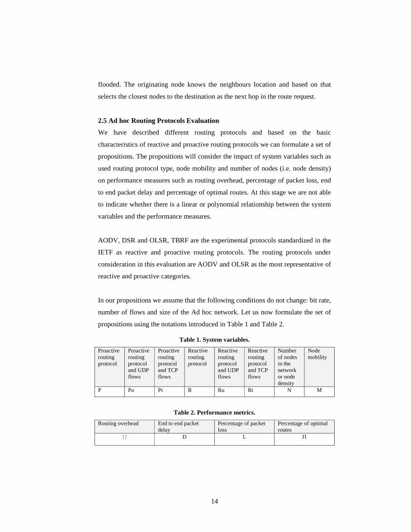
In our propositions we assume that the following conditions do not change: bit rate,
number of flows and size of the Ad hoc network. Let us now formulate the set of
propositions using the notations introduced in Table 1 and Table 2.
Table 1. System variables.
Proactive routing protocol
Proactive routing protocol and UDP flows
Proactive routing protocol and TCP flows
Reactive routing protocol
Reactive routing protocol and UDP flows
Reactive routing protocol and TCP flows
Number of nodes in the network or node density
Node mobility
P Pu Pt R Ru Rt N M
Table 2. Performance metrics.
Routing overhead End to end packet delay
Percentage of packet loss
Percentage of optimal routes
W D L Π
15
Proposition 1. Routing overhead increases with node mobility in both
proactive and reactive routing protocols.
P1.1 For M1>M2, ΩP(M1)>ΩP(M2)
P1.2 For M1>M2, ΩR(M1)>ΩR(M2)
P1.3 For M>Mthreshold, ΩP(M)> ΩR(M) ≥0
M1 and M2 represent different values for mobility. The derivatives ΩP´(M)≥0 and
ΩR´(M)≥0 are used to demonstrate that overhead function increases with mobility,
and they will be applied for the mathematical analysis in the rest of the chapter.
The routing overhead increases with node mobility due to the extra route discovery
transactions generated in reactive protocols and the route updates required in
proactive routing protocols. We expect that the routing overhead of proactive
routing protocols increases more than the routing overhead of reactive protocols
because the route updates need to span all nodes when links break due to mobility.
We assume that the routing overhead of reactive routing protocols is lower than the
routing overhead of proactive protocols because only the existing routes need to be
re-established during a link break.
Proposition 2. End to end packet delay increases with node mobility in both
proactive and reactive routing protocols.
P2.1 For M1>M2, DP(M1)>DP(M2)
P2.2 For M1>M2, DR(M1)>DR(M2)
P2.3 For M>Mthreshold, DP(M)>DR(M)≥0
M1 and M2 represent different values for mobility. The derivatives DP´(M)≥0 and
DR´(M)≥0 are used to demonstrate that delay function increases with mobility, and
they will be applied for the mathematical analysis in the rest of the chapter.
In proactive routing protocols, the end to end packet delay increases when there is
network congestion because of the increment in the number of transactions
16
required to exchange topology information with all the nodes. The end to end
packet delay increases with node mobility in reactive routing protocols because of
the increment of route discovery transactions. We expect that the packet delay in
reactive routing protocols is lower than in proactive protocols because the route
information is fresh since it is acquired right before starting the flow. We assume
that the packet delay in proactive routing protocols is higher than in reactive
protocols because the routing information may be stale when starting the packet
flow, and the link breaks due to mobility create additional traffic increasing the
congestion in all nodes.
Proposition 3. Percentage of packet loss increases with node mobility in both
proactive and reactive protocols.
P3.1 For M1>M2, LP(M1)>LP(M2)
P3.2 For M1>M2, LR(M1)>LR(M2)
P3.3 For M>Mthreshold, LP(M)>LR(M)>0
M1 and M2 represent different values for mobility. The derivatives LP´(M)≥0 and
LR´(M)≥0 are used to demonstrate that packet loss function increases with
mobility, and they will be applied for the mathematical analysis in the rest of the
chapter.
When mobility increases, links are more frequently broken and percentage of
packet loss increases. We expect the mobility will increase the link breaks that in
proactive protocols will result in additional traffic and congestion in all nodes. The
reactive protocols have more fresh routing information when starting the packet
flow that will result in lower packet loss than in proactive protocols.
Proposition 4. Percentage of optimal routes decreases in both proactive and
reactive routing protocols when node mobility increases.
P4.1 For M1>M2, ΠP(M1)<ΠP(M2)
17
P4.2 For M1>M2, ΠR(M1)<ΠR(M2)
M1 and M2 represent different values for mobility. The derivatives ΠP´(M)≤0 and
ΠR´(M) ≤0 are used to demonstrate that optimal routes function decreases with
mobility, and they will be applied for the mathematical analysis in the rest of the
chapter.
When the nodes move new shorter routes may appear and it takes time for a
routing protocol to discover those optimal routes. This problem occurs more often
when node mobility increases.
Proposition 5. Percentage of optimal routes obtained with proactive routing
protocols is higher than with reactive protocols.
P5.1 ΠP(M)>ΠR(M)
The routing protocols obtain the network topology based on periodic routing
updates (i.e. proactive) or on demand route discovery (i.e. reactive). The proactive
routing protocols apply an additional algorithm over the discovered routes to select
the most optimal route (e.g. lower number of hops). As a consequence, proactive
routing protocols obtain a higher percentage of optimal routes compared to the
routes obtained with reactive routing protocols. When mobility increases, the
routes obtained become stale due to frequent link brakes.
Proposition 6. Routing overhead increases with the number of nodes in both
proactive and reactive routing protocols.
P6.1 For N1>N2, ΩP(N1)>ΩP(N2)
P6.2 For N1>N2, ΩR(N1)>ΩR(N2)
N1 and N2 represent different values for the number of nodes. The derivatives
ΩP´(N) ≥0 and ΩR´(N) ≥0 are used to demonstrate that routing overhead function
18
increases with the number of nodes, and they will be applied for the mathematical
analysis in the rest of the chapter.
The proactive routing protocols have to share the routing information with all the
other nodes in the network, which increases the routing information per node as a
function of the total number of nodes in the network. The reactive routing protocols
have to increase the TTL in the route request to reach all the nodes in the network.
Therefore, when the node density increases the route requests are sent by higher
number of nodes but few of the messages are reaching new nodes, thus decreasing
the route discovery efficiency.
Proposition 7. For the same number of nodes and mobility conditions the
routing overhead is higher in proactive than in reactive protocols.
P7.1 ΩP(M,N)≥ΩR(M,N)
The routing overhead increases with the number of nodes due to additional
topology information required in proactive protocols, and the additional route
requests forwarded by each of the intermediate nodes in reactive protocols.
Proposition 8. End to end packet delay increases with the number of nodes in
both proactive and reactive routing protocols.
P8.1 For N1>N2, DP(N1)>DP(N2)
P8.2 For N1>N2, DR(N1)>DR(N2)
N1 and N2 represent different values for the number of nodes. The derivatives
DP´(N) ≥0 and DR´(N) ≥0 are used to demonstrate that delay function increases
with the number of nodes, and they will be applied for the mathematical analysis in
the rest of the chapter.
In this proposition, N denotes both the density and the number of nodes on the end
to end path.
19
Proposition 9. Percentage of packet loss increases with the number of nodes in
both proactive and reactive routing protocols.
P9.1 For N1>N2, LP(N1)>LP(N2)
P9.2 For N1>N2, LR(N1)>LR(N2)
N1 and N2 represent different values for the number of nodes. The derivatives
LP´(N) ≥0 and LR´(N) ≥0 are used to demonstrate that packet loss function
increases with the number of nodes, and they will be applied for the mathematical
analysis in the rest of the chapter.
When the number of nodes increases, the network gets congested because of the
additional signalling, causing an increment of the packet delay and the percentage
of packet loss. According to Proposition 1, the routing overhead increases with
mobility, therefore the throughput will decrease reducing the available bandwidth
and increasing the percentage of packet loss.
Proposition 10. Percentage of optimal routes obtained with proactive and
reactive routing protocols decreases with the number of nodes.
P10.1 For N1>N2, ΠP(N1)<ΠP(N2)
P10.2 For N1>N2, ΠR(N1)<ΠR(N2)
N1 and N2 represent different values for the number of nodes. The derivatives
ΠP´(N)≤0 and ΠR´(N)≤0 are used to demonstrate that optimal routes function
decreases with the number of nodes, and they will be applied for the mathematical
analysis in the rest of the chapter.
When calculating the optimal routes, increasing the number of nodes will decrease
the efficiency of the protocols because of the additional topology information
collected from all the nodes that has to be processed.
20
2.6 Proactive versus Reactive Simulation Comparison
In previous section we have formulated a number of propositions based on our
qualitative understanding of the behaviour of ad hoc routing protocols. In this
section, we include results from a large set of simulations and in section 2.8 we
provide the measurements obtained from our test bed to seek confirmation of the
accuracy of our propositions. In order to make the transformation from quantitative
numeric results obtained from simulations to qualitative statements we fit the
simulation results into parametric equations that minimize approximation error.
The purpose of the parametric equations is not to reflect the behaviours of all Ad
hoc networks under certain conditions. However, the goal is to explore the
behaviour of Ad hoc networks under different routing protocols qualitatively in
order to have a good understanding of the design tradeoffs of routing protocols.
Therefore, we use both simulations and measurements to study the behaviour.
Based on our own experience, we consider that too many simulation results have
been published that fit poorly to the measured behaviour gained from a test bed or
a real network. The limitation of measurements, on the other hand, is that
generalizing the results is difficult. Therefore, we do not believe it would be
possible to propose a grand theory and verify it with the means in our disposal.
However, our aim is to improve on routing protocol design and justify design
choices without having such a theory by using both measurements and simulations,
by explaining the differences between the two and thus verifying our work on a
qualitative level.
In this section, simulation results justifying the advantages and drawbacks of the
reactive and proactive Ad hoc routing protocols will be presented [15]. The routing
protocols comparison has been done using ns-2 simulator [43] version 2.27 with
standard IEEE 802.11 MAC protocol, which is used in the simulations and test bed
included in this thesis. We also verify some of the propositions introduced in
section 2.5
21
The results are obtained from the average of three simulations rounds performed
continuously in order to reduce any possible effect due to initialization process of
the simulator. In the simulations we consider the following parameters:
- Simulation area: 1500m x 300m.
- Simulation time: 900 seconds.
- Traffic flows:
1. Constant Bit Rate (CBR) with UDP transport: 20 IP unidirectional
flows.
2. Traffic with TCP transport: 20 IP unidirectional flows.
- Connection rate: 8 packets/second.
- Packet size: 65 bytes.
- Number of nodes: 50 nodes using random waypoint mobility pattern.
- Pause time between node movements: 0, 30, 60, 120, 300, 600 and 900
seconds.
In the simulations we consider the mobility as the average speed of the node during
the simulation.
simulation
moving
simulation
pausemoving
t
tM
t
ttMM maxmax 0
=+
= where simulationmoving tt
MM=
= max and 0
0=
=movingt
M .
We run simulations with the same parameters but using either UDP or TCP as
transport protocol for the traffic flows to compare the effect of congestion and
reliable traffic control mechanisms.
The literature shows that different mobility patterns affect Ad hoc networks
performance results [44]. Ad hoc networks will be deployed under different
mobility patterns and the routing protocols have to perform in different
environments. Therefore, in the simulations, the nodes follow a different mobility
pattern after each waiting time as characterised in the random waypoint model1
[45].
1 It has been demonstrated that the random waypoint model is not the most accurate mobility pattern but we will use it for simplicity assuming that it is good enough.
22
The simulations are made considering that the network is handling the traffic
generated by 20 active connections transmitting 8 packets/second. The simulations
reflect the performance of Ad hoc networks with real time applications under
different mobility conditions and using different routing and transport protocols.
The simulations last for 900 seconds, thus a pause time of 900 seconds is
equivalent to static nodes that do not move during the simulation.
Both reactive (i.e. AODV, TORA, DSR) and proactive routing protocols (i.e.
DSDV, OLSR) are covered in the simulations. The simulation results presented in
this section are inaccurate due to the random behaviour of the nodes. Therefore, a
deeper analysis will be made extracting from each simulation the associated
equation for the most representative reactive (i.e. AODV) and proactive (i.e.
OLSR) routing protocols and specific transport protocol (i.e. TCP or UDP).
The simulation results can be associated with an equation that can be
linear bcxxf +=)( , polynomial nn xcxcxcbxf ++++= ...)( 2
21, logarithmic
bxcxf += ln)( or exponential bxcexf =)( . The constants c and b of these
equations are adjusted using the r-squared value ( )( )
∑∑
∑
−
−−=
n
YY
YYr
ii
ii
2
2
2
2ˆ
1, where iY
represents the value obtained in the simulation and iY represents the estimated
value from the associated equation. The r-squared value represents the
approximation error, thus it tends to 1 when the values from the simulation and the
associated equation match. In following sections each simulation is associated with
the equation that provides the lowest approximation error 2r .
2.6.1 Simulation Results on Mobility
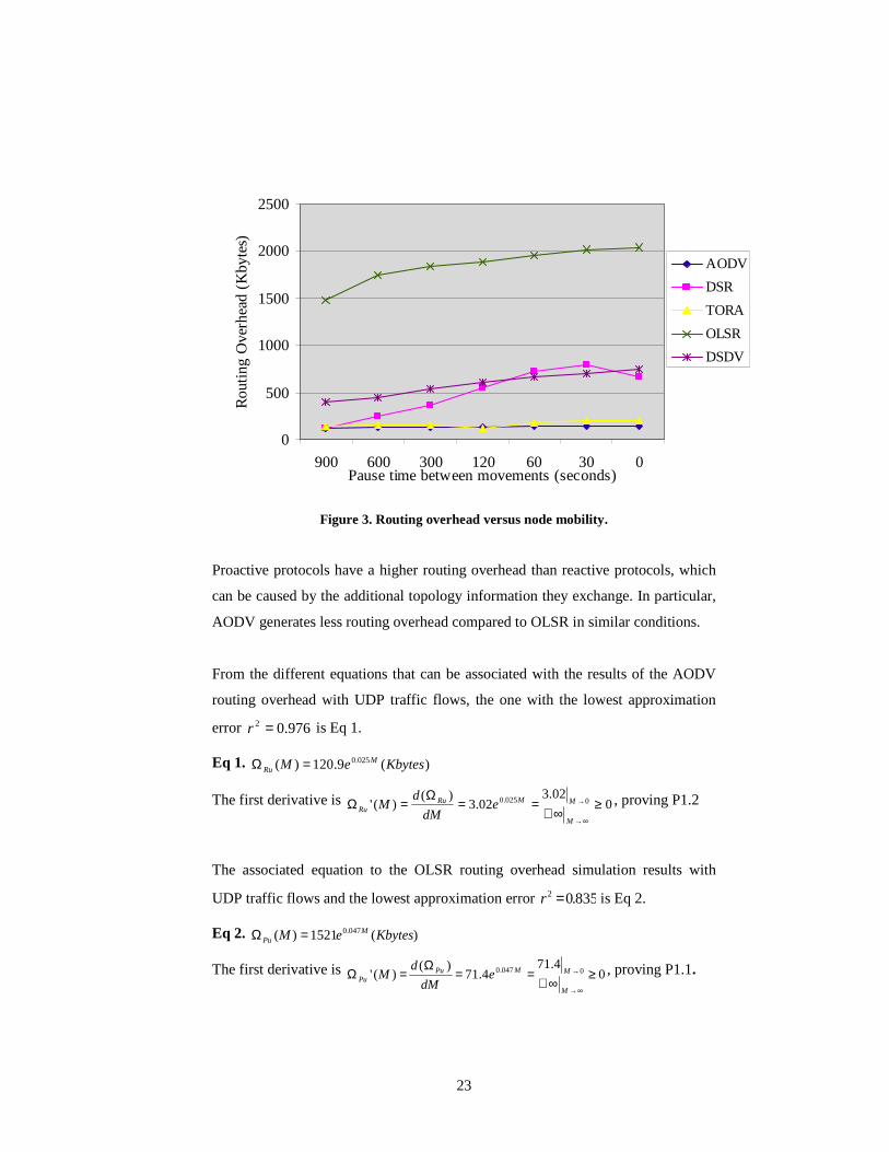
Figure 3 shows the routing overhead generated by reactive and proactive routing
protocols during the simulation time versus node mobility with UDP traffic flows.
23
0
500
1000
1500
2000
2500
900 600 300 120 60 30 0Pause time between movements (seconds)
Ro
utin
g O
verh
ead
(K
byte
s)
AODV
DSR
TORA
OLSR
DSDV
Figure 3. Routing overhead versus node mobility.
Proactive protocols have a higher routing overhead than reactive protocols, which
can be caused by the additional topology information they exchange. In particular,
AODV generates less routing overhead compared to OLSR in similar conditions.
From the different equations that can be associated with the results of the AODV
routing overhead with UDP traffic flows, the one with the lowest approximation
error 976.02 =r is Eq 1.
Eq 1. )(9.120)( 025.0 KbyteseM MRu =Ω
The first derivative is 002.3
02.3)(
)(' 0025.0 ≥∞+
==Ω
=Ω∞→
→
M
MMRuRu e
dM
dM , proving P1.2
The associated equation to the OLSR routing overhead simulation results with
UDP traffic flows and the lowest approximation error 835.02 =r is Eq 2.
Eq 2. )(1521)( 047.0 KbyteseM MPu =Ω
The first derivative is 04.71
4.71)(
)(' 0047.0 ≥∞+
==Ω
=Ω∞→
→
M
MMPuPu e
dM
dM , proving P1.1.
24
Figure 4 shows the routing overhead in AODV and OLSR using a transport
protocol that includes reliability and congestion mechanisms such as TCP. The
routing overhead increases in both AODV and OLSR compared to UDP traffic
flows.
0
5001000
15002000
2500
30003500
40004500
5000
900 600 300 120 60 30 0Pause time between movements (seconds)
Rou
ting
Ove
rhea
d (
Kb
ytes
)
AODV/UDP
AODV/TCP
OLSR/UDP
OLSR/TCP
Figure 4. Routing overhead versus node mobility and transport protocol.
From the different equations that can be associated with the results of the AODV
routing overhead with TCP traffic flows, the one with the lowest approximation
error 456.02 =r is Eq 3.
Eq 3. )(1.2813)( 022.0 KbyteseM MRt =Ω
The first derivative is 088.61
88.61)(
)(' 0022.0 ≥∞+
==Ω
=Ω∞→
→
M
MMRtRt e
dM
dM , proving P1.2.
The associated equation to the OLSR routing overhead simulation results with TCP
traffic flows and the lowest approximation error 244.02 =r is Eq 4.
Eq 4. )(7.4014)( 013.0 KbyteseM MPt =Ω
The first derivative is 019.52
19.52)(
)(' 0013.0 ≥∞+
==Ω
=Ω∞→
→
M
MMPtPt e
dM
dM , proving
P1.1 and P1.3.
25
The associated equations to AODV and OLSR using UDP are more accurate than
the same equations when using TCP (i.e. higher r-squared value) and they show
that proactive protocols have higher routing overhead than reactive protocols under
similar conditions, as stated in P1.3.
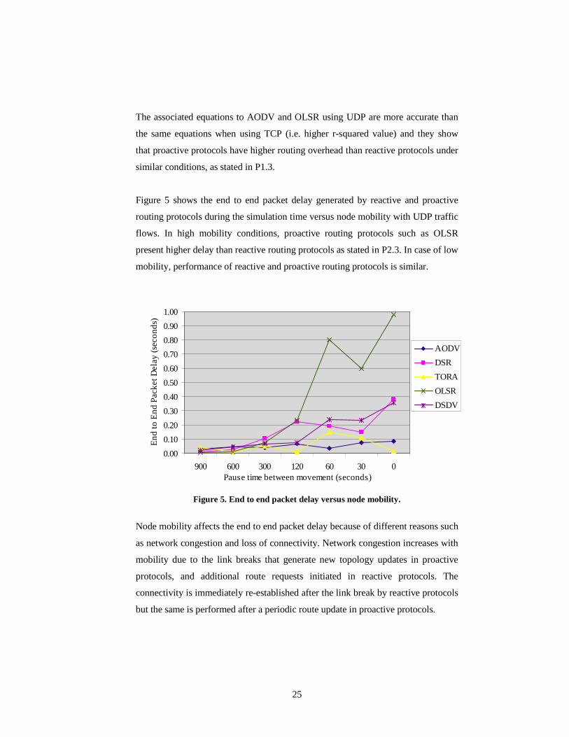
Figure 5 shows the end to end packet delay generated by reactive and proactive
routing protocols during the simulation time versus node mobility with UDP traffic
flows. In high mobility conditions, proactive routing protocols such as OLSR
present higher delay than reactive routing protocols as stated in P2.3. In case of low
mobility, performance of reactive and proactive routing protocols is similar.
0.00
0.10
0.20
0.30
0.40
0.50
0.60
0.70
0.80
0.90
1.00
900 600 300 120 60 30 0Pause time between movement (seconds)
En
d t
o E
nd
Pa
cke
t D
ela
y (s
eco
nd
s)
AODV
DSR
TORA
OLSR
DSDV
Figure 5. End to end packet delay versus node mobility.
Node mobility affects the end to end packet delay because of different reasons such
as network congestion and loss of connectivity. Network congestion increases with
mobility due to the link breaks that generate new topology updates in proactive
protocols, and additional route requests initiated in reactive protocols. The
connectivity is immediately re-established after the link break by reactive protocols
but the same is performed after a periodic route update in proactive protocols.
26
The associated equation to the AODV end to end packet delay simulation results
with UDP traffic flows and the lowest approximation error 625.02 =r is Eq 5.
Eq 5. )(021.0008.0)( sMMDRu +=
The first derivative is 0008.0)(
)(' ≥==dM
DdMD Ru
Ru, proving P2.2.
The associated equation to the OLSR end to end packet delay simulation results
with UDP traffic flows and the lowest approximation error 851.02 =r is Eq 6.
Eq 6. )(302.0172.0)( sMMDPu −=
The first derivative is 0172.0)(
)(' ≥==dM
DdMD Pu
Pu, proving P2.1.
In Eq 6 when M=0 we obtain a negative value for the end to end packet delay
302.0)0( −=PuD representing an approximation error.
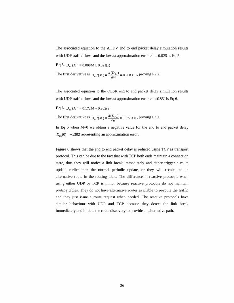
Figure 6 shows that the end to end packet delay is reduced using TCP as transport
protocol. This can be due to the fact that with TCP both ends maintain a connection
state, thus they will notice a link break immediately and either trigger a route
update earlier than the normal periodic update, or they will recalculate an
alternative route in the routing table. The difference in reactive protocols when
using either UDP or TCP is minor because reactive protocols do not maintain
routing tables. They do not have alternative routes available to re-route the traffic
and they just issue a route request when needed. The reactive protocols have
similar behaviour with UDP and TCP because they detect the link break
immediately and initiate the route discovery to provide an alternative path.
27
0.00
0.20
0.40
0.60
0.80
1.00
900 600 300 120 60 30 0Pause time between movements (seconds)
En
d to
End
Pac
ket
Del
ay (
seco
nds
)
AODV/UDP
AODV/TCP
OLSR/UDP
OLSR/TCP
Figure 6. End to end packet delay versus node mobility and transport protocol.
The associated equation to the AODV end to end packet delay simulation results
with TCP traffic flows and the lowest approximation error 26.02 =r is Eq 7.
Eq 7. )(127.00025.0)( sMMDRt +=
The first derivative is 00003.0)(
)(' ≥==dM
DdMD Rt
Rt, proving P2.2.
The associated equation to the OLSR end to end packet delay simulation results
with TCP traffic flows and the lowest approximation error 44.02 =r is Eq 8.
Eq 8. )(1619.00076.0)( sMMDPt +=
The first derivative is 00012.0)(
)(' ≥==dM
DdMD Pt
Pt, proving P2.1.
In proactive protocols, the connection control in the traffic flow decreases the delay
compared to non reliable connections when using UDP as transport protocol. The
accuracy of the associated equations for UDP traffic flows is higher than the
equations for TCP flows, but still they show that the end to end packet delay is
higher in proactive routing than in reactive routing protocols as stated in P2.3.
28
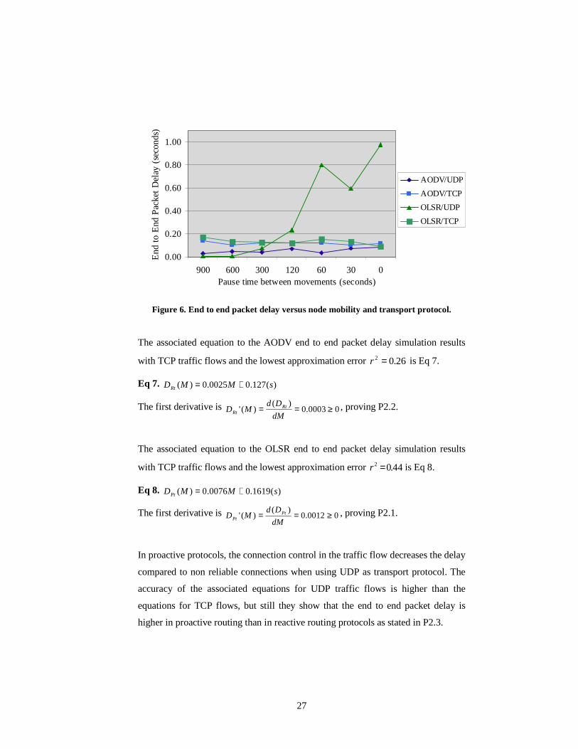
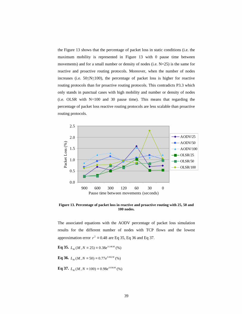
Figure 7 shows the percentage of packet loss generated when reactive or proactive
routing protocols are used during the simulation time versus node mobility with
UDP traffic flows.
0
5
10
15
20
25
30
35
40
900 600 300 120 60 30 0
Pause between movements (seconds)
Pa
cke
t L
oss
(%
) AODV
DSR
TORA
OLSR
DSDV
Figure 7. Percentage of packet loss versus node mobility.
We measured the packet loss as the percentage of packets that did not reach the
destination from the total number of packets sent. The percentage of packet loss is
higher in case of proactive routing protocols than in case of reactive routing
protocols and increases with mobility as stated in Proposition 3.
The associated equation to the AODV percentage of packet loss simulation results
with UDP traffic flows and the lowest approximation error 881.02 =r is Eq 9.
Eq 9. (%)083.0)( 455.0 MRu eML =
The first derivative is 0038.0
038.0)(
)(' 0455.0 ≥∞+
===∞→
→
M
MMRuRu e
dM
LdML , proving P3.2.
The associated equation to the OLSR percentage of packet loss simulation results
with UDP traffic flows and the lowest approximation error 56.02 =r is Eq 10.
Eq 10. (%)225.0)( 89.0 MPu eML =
29
The first derivative is 02.0
2.0)(
)(' 089.0 ≥∞+
===∞→
→
M
MMPuPu e
dM
LdML , proving P3.1.
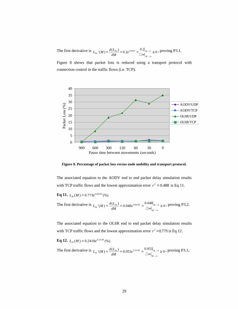
Figure 8 shows that packet loss is reduced using a transport protocol with
connection control in the traffic flows (i.e. TCP).
0
5
10
15
20
25
30
35
40
900 600 300 120 60 30 0Pause time between movements (seconds)
Pac
ket
Lo
ss (
%)
AODV/UDP
AODV/TCP
OLSR/UDP
OLSR/TCP
Figure 8. Percentage of packet loss versus node mobility and transport protocol.
The associated equation to the AODV end to end packet delay simulation results
with TCP traffic flows and the lowest approximation error 488.02 =r is Eq 11.
Eq 11. (%)773.0)( 062.0 MRt eML =
The first derivative is 0048.0
048.0)(
)(' 0062.0 ≥∞+
===∞→
→
M
MMRtRt e
dM
LdML , proving P3.2.
The associated equation to the OLSR end to end packet delay simulation results
with TCP traffic flows and the lowest approximation error 779.02 =r is Eq 12.
Eq 12. (%)2418.0)( 221.0 MPt eML =
The first derivative is 0053.0
053.0)(
)(' 0221.0 ≥∞+
===∞→
→
M
MMPtPt e
dM
LdML , proving P3.1.
30
TCP includes a connection control mechanism that reduces the end to end packet
delay as we can see comparing Eq 6 with Eq 8 and it reduces packet loss as we can
deduce from Eq 10 and Eq 12. Lower slopes in Eq 11 than in Eq 12 demonstrate
that reactive protocols present shorter end to end packet delay than proactive
routing protocols, proving P3.3.
Figure 9 shows the percentage of optimal routes obtained by reactive and proactive
routing protocols during the simulation time versus node mobility. Proactive
routing protocols perform better than reactive routing protocols when obtaining the
optimal routes. Proactive routing protocols maintain the routing information up to
date and apply appropriate routing algorithms (e.g. Shortest Path [40]). The
percentage of optimal routes decreases in both reactive and proactive protocols
with node mobility as stated in Proposition 4.
60
70
80
90
100
900 600 300 120 60 30 0Pause time between movements (seconds)
Opt
imal
Rou
tes
(%)
AODV
DSR
TORA
OLSR
DSDV
Figure 9. Percentage of optimal routes versus node mobility.
The associated equation to the AODV percentage of optimal routes simulation
results with UDP traffic flows and the lowest approximation error 729.02 =r is Eq
13.
Eq 13. )(%)ln(864.2028.94)( MMRu −=Π
31
The first derivative is 00
864.2)()(' 0 ≤
−∞−
=−=Π
=Π∞→
→
M
MRuRu MdM
dM , proving P4.2.
The associated equation to the OLSR percentage of optimal routes simulation
results with UDP traffic flows and the lowest approximation error 902.02 =r is Eq
14.
Eq 14. )(%)ln(381.2100)( MMPu −=Π
The first derivative is 00
381.2)()(' 0 ≤
−∞−
=−=Π
=Π∞→
→
M
MPuPu MdM
dM , proving P4.1.
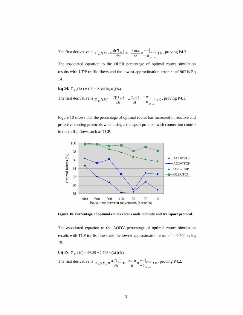
Figure 10 shows that the percentage of optimal routes has increased in reactive and
proactive routing protocols when using a transport protocol with connection control
in the traffic flows such as TCP.
88
90
92
94
96
98
100
900 600 300 120 60 30 0Pause time between movements (seconds)
Opt
imal
Rou
tes
(%)
AODV/UDP
AODV/TCP
OLSR/UDP
OLSR/TCP
Figure 10. Percentage of optimal routes versus node mobility and transport protocol.
The associated equation to the AODV percentage of optimal routes simulation
results with TCP traffic flows and the lowest approximation error 504.02 =r is Eq
15.
Eq 15. )(%)ln(708.285.96)( MMRt −=Π
The first derivative is 00
708.2)()(' 0 ≤
−∞−
=−=Π
=Π∞→
→
M
MRtRt MdM
dM , proving P4.2.
32
The associated equation to the OLSR percentage of optimal routes simulation
results with TCP traffic flows and the lowest approximation error 591.02 =r is Eq
16.
Eq 16. )(%)ln(7653.0100)( MMPt −=Π
The first derivative is 00
7653.0)()(' 0 ≤
−∞−
=−=Π
=Π∞→
→
M
MPtPt MdM
dM , proving P4.1.
The associated equations show that 100% of the routes obtained with the proactive
protocol can be optimal in case of zero node mobility compared to the case of
reactive protocol where with similar conditions only 94% of the routes obtained are
optimal, which proves Proposition 5. We can see that using a connection control
transport protocol increases the percentage of optimal routes in reactive ( Eq 13, Eq
15) and proactive (Eq 14, Eq 16) protocols. When the connection control detects a
link break, it triggers either a route recalculation in proactive protocols or a route
discovery in reactive protocols. However, proactive protocols obtain a higher
percentage of optimal routes than reactive protocols as stated in P5.1.
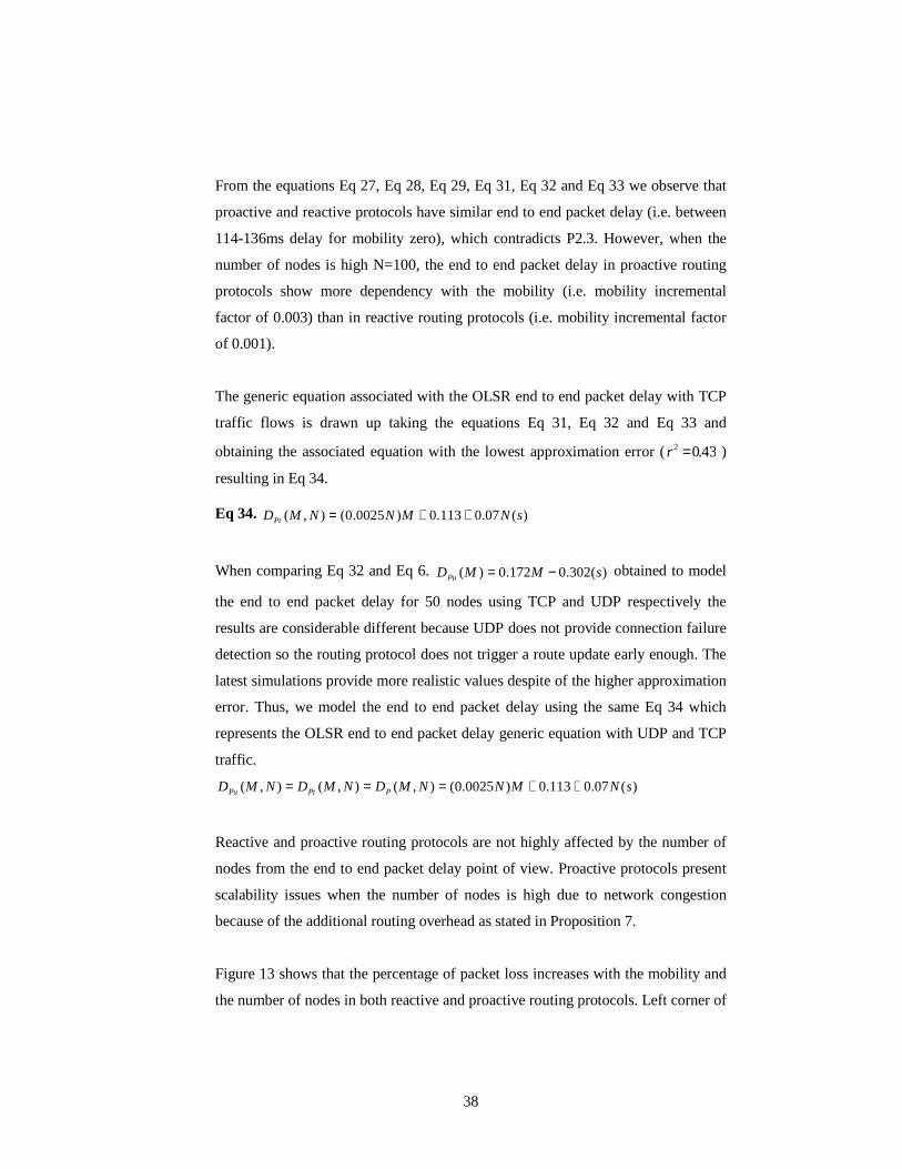
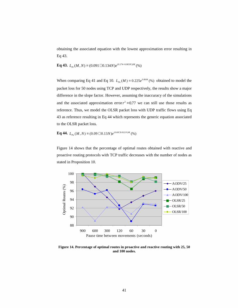
2.6.2 Simulation Results on Scalability
We have verified some of the propositions based on the results from the
simulations but the scalability effect on the routing protocols when increasing the
number or density of nodes remains to be demonstrated. The simulator has some
limitations in terms of number of nodes (i.e. max number of nodes is 100).
Therefore, in order to study the impact on the performance results when increasing
the number of nodes, new simulations were performed with 25, 50 and 100 nodes
keeping the same value for the rest of the parameters. We select TCP as the
transport protocol for these simulations because it provides similar results for
proactive and reactive protocols regarding end to end packet delay and packet loss.
However, we have to consider that the connection control mechanism in TCP
creates additional overhead.
33
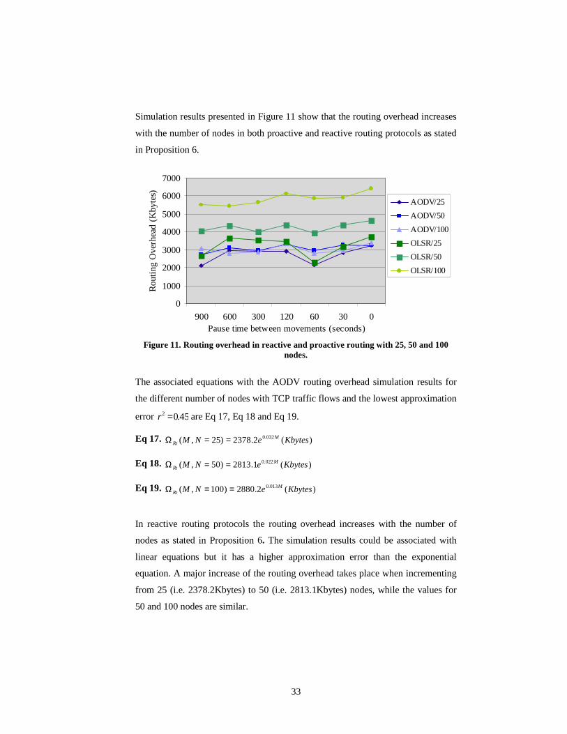
Simulation results presented in Figure 11 show that the routing overhead increases
with the number of nodes in both proactive and reactive routing protocols as stated
in Proposition 6.
0
1000
2000
3000
4000
5000
6000
7000
900 600 300 120 60 30 0Pause time between movements (seconds)
Rou
ting
Ove
rhea
d (K
byte
s)
AODV/25
AODV/50
AODV/100
OLSR/25
OLSR/50
OLSR/100
Figure 11. Routing overhead in reactive and proactive routing with 25, 50 and 100
nodes.
The associated equations with the AODV routing overhead simulation results for
the different number of nodes with TCP traffic flows and the lowest approximation
error 45.02 =r are Eq 17, Eq 18 and Eq 19.
Eq 17. )(2.2378)25,( 032.0 KbyteseNM MRt ==Ω
Eq 18. )(1.2813)50,( 022.0 KbyteseNM MRt ==Ω
Eq 19. )(2.2880)100,( 013.0 KbyteseNM MRt ==Ω
In reactive routing protocols the routing overhead increases with the number of
nodes as stated in Proposition 6. The simulation results could be associated with
linear equations but it has a higher approximation error than the exponential
equation. A major increase of the routing overhead takes place when incrementing
from 25 (i.e. 2378.2Kbytes) to 50 (i.e. 2813.1Kbytes) nodes, while the values for
50 and 100 nodes are similar.
34
Next, we define a generic equation that includes both mobility and the number of
nodes as variables. We take the equations obtained from simulations for 25, 50 and
100 nodes, with mobility as the only variable, and we associate them with an
equation that can be linear, polynomial, logarithmic or exponential depending on
the associated error. The generic equation associated to the AODV routing
overhead with TCP traffic flows is drawn up taking the equations Eq 17, Eq 18, Eq
19 and obtaining the associated equation for the bases (i.e. 2378.2, 2813.1 and
2880.2) and the slope factors (i.e. 0.032, 0.022 and 0.013) with the lowest
approximation error resulting in Eq 20.
Eq 20. )()2512188(),( )009.004.0( KbyteseNNM MNRt
++=Ω
When comparing Eq 18 and Eq 1. )(9.120)( 025.0 KbyteseM MRu =Ω obtained to model
the routing overhead for 50 nodes using TCP and UDP respectively, we see that the
results are different. This is due to the additional overhead in TCP compared to
UDP. To model the routing overhead using UDP considering as variables the
mobility and the number of nodes, we take Eq 20 and Eq 18 as reference to
estimate the generic equation associated to the AODV routing overhead with UDP.
The base of the equation with TCP changes from 2188 in Eq 18 to 2813.1 in Eq 20
which means an increment of 28.57% so we can estimate that for UDP it will be
)(4.155),( 025.0 KbyteseNM MRu =Ω . The slope of the equation changes from 0.022 in
Eq 18 to 0.04 in Eq 20 which means an increment of 81.82% so we estimate that
for UDP it will be )(4.155),( 045.0 KbyteseNM MRu =Ω . The slope we obtain with
UDP is similar to the one in Eq 20 so we could extend the factor associated with N
for UDP with the same value for TCP as in Eq 20. We estimate that for UDP the
final slope is )(4.155),( )009.0045.0( KbyteseNM MNRu
+=Ω . The base of Eq 18 for TCP is
2813.1 which is 23.27 times bigger than the base of Eq 1 for UDP. Therefore, we
use the factor associated with N for TCP in Eq 20 as reference (i.e. 120N) to
estimate a similar value for UDP. Thus, we model the routing overhead for UDP
taking Eq 18, Eq 20 and Eq 1 as reference, resulting in Eq 21 which represents the
AODV routing overhead generic equation with UDP traffic.
1 Requires maintaining in the cache only the most recently used routes. 2 Requires maintaining tables with entries for all the nodes in the network. 3 Requires additional route discovery and maintenance that increases with high mobility. 4 Routing information is periodically maintained up to date in all the nodes.
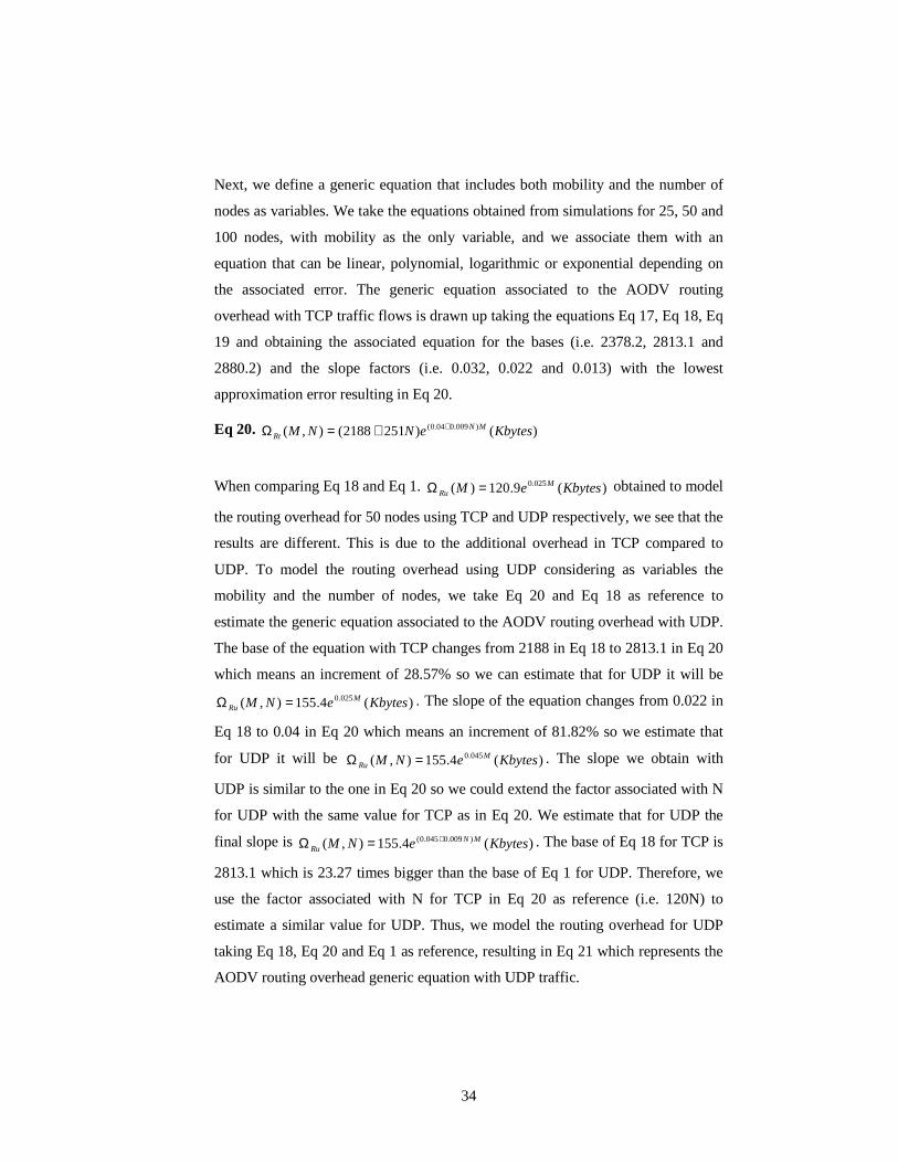
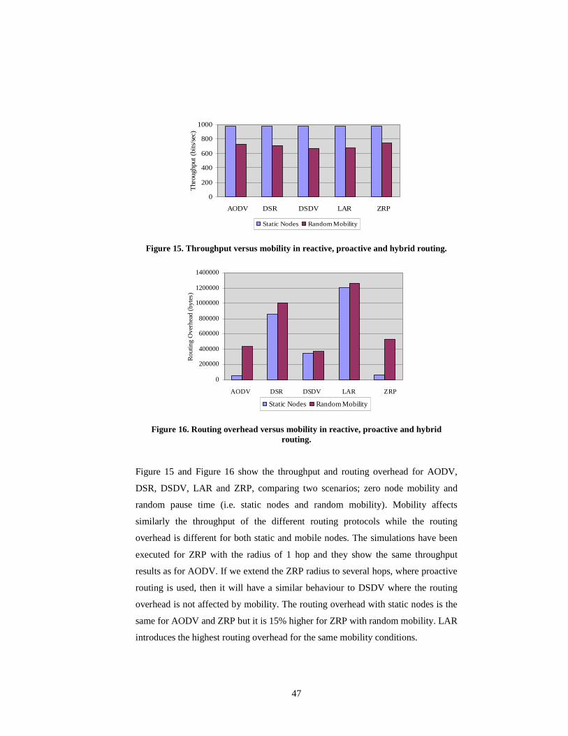
2.7 Ad hoc Routing Protocols Simulation Conclusions
The reactive routing protocols under analysis have clear drawbacks such as the
excessive flooding traffic in the route discovery and the route acquisition delay.
When the network is congested, the routing information is lost and a consecutive
set of control packets are issued to re-establish the links, increasing the routing
latency (i.e. time the routing protocol requires for obtaining the route to the
destination node) and percentage of packet loss. If the Hello messages are not
received, then error requests are issued and new route requests are sent to re-
establish the link. Thus, the reactive protocols do not scale when the load and node
density increase. Moreover, the reactive routing protocols do not have knowledge
about the QoS in the path before the route is established and the routes are not
optimised.
The reactive routing protocols suffer from high routing latency and percentage of
packet loss, which increase with mobility and large networks. The percentage of
optimal routes calculated with reactive protocols is lower than in proactive
protocols and it decreases in large networks. An advantage of reactive protocols
45
like AODV is that they maintain only the active routes in the routing table, which
minimizes the memory required in the node. Moreover, the protocol itself is simple
so the computational requirements are minimal, extending the lifetime of the node
in the Ad hoc network. The routing overhead is equivalent to additional packet
processing, thus reactive protocols will have lower power consumption than
proactive protocols. In simulations with a small number of nodes, AODV has lower
percentage of packet loss than OLSR. Therefore in networks with light traffic and
low mobility reactive protocols are scalable because of the small bandwidth and
storage requirements.
The proactive routing protocols under analysis maintain topology information up to
date with periodic update messages. The proactive routing protocols minimize the
route discovery delay, which minimizes the percentage of packet loss since the
routes are known in advance and no additional routing overhead and processing are
required. However, under high mobility conditions more and more routes
established based on the previous periodic update become stale leading to an
increased percentage of packet loss.
The proactive routing protocols have low routing latency since all the routes are
available immediately even in large networks. The proactive routing protocols
calculate the most optimal routes since they apply hop count based routing
algorithms. The proactive routing protocols have higher percentage of packet loss
than reactive protocols in networks with reduced number of nodes and high
mobility as depicted in Figure 7. However, if the transport protocol includes
connection control mechanism (i.e. TCP) that detects link breaks and triggers route
update or route recalculation, then proactive protocols present lower percentage of
packet loss than reactive protocols as depicted in Figure 13.
A drawback of proactive routing protocols is that they require a constant bandwidth
and cause a processing overhead to maintain the routing information up to date.
This overhead increases with the number of nodes and mobility since the updates
have to be more frequent to maintain accurate routing information. The proactive
46
routing protocols have lower routing latency but they do not react quickly enough
to topology changes. The proactive routing protocols have been enhanced towards
hybrid and hierarchical solutions to deal with this scalability problem in Ad hoc
networks. OLSR reduces the control and processing overhead by selecting some
nodes (i.e. Multipoint Relay nodes) within the network to maintain the routing
information. The link information updates are propagated between MPR nodes
only, reliving the rest of the nodes from participating in the topology maintenance.
Other optimizations consist of exchanging only the differential updates,
implementing hybrid solutions such as ZRP [41] that combines reactive and
proactive routing protocols or routing protocols that use the nodes location data
such as LAR [42].
In order to analyse the performance of the hybrid protocols versus reactive and
proactive, we run additional simulations in the ns-2 with similar parameters.
- Simulation area: 1500m x 300m.
- Transmitter range: 250m and 2Mbit bandwidth.
- Simulation time: 900 seconds.
- Constant Bit Rate (CBR) traffic with UDP transport: 15 IP unidirectional
connections.
- Connection rate: 5 packets/second.
- Packet size: 65 bytes.
- Number of nodes: 50 nodes using random waypoint mobility pattern.
- Pause time between node movements: 0, 30, 60, 120, 300, 600 and 900
seconds.
Figure 15 and Figure 16 show the results of the additional simulations run
including hybrid routing.
47
0
200
400
600
800
1000
AODV DSR DSDV LAR ZRP
Thro
ughput (b
its/s
ec)
Static Nodes Random Mobility
Figure 15. Throughput versus mobility in reactive, proactive and hybrid routing.
0
200000
400000
600000
800000
1000000
1200000
1400000
AODV DSR DSDV LAR ZRP
Ro
utin
g O
verh
ead
(byt
es)
Static Nodes Random Mobility
Figure 16. Routing overhead versus mobility in reactive, proactive and hybrid routing.
Figure 15 and Figure 16 show the throughput and routing overhead for AODV,
DSR, DSDV, LAR and ZRP, comparing two scenarios; zero node mobility and
random pause time (i.e. static nodes and random mobility). Mobility affects
similarly the throughput of the different routing protocols while the routing
overhead is different for both static and mobile nodes. The simulations have been
executed for ZRP with the radius of 1 hop and they show the same throughput
results as for AODV. If we extend the ZRP radius to several hops, where proactive
routing is used, then it will have a similar behaviour to DSDV where the routing
overhead is not affected by mobility. The routing overhead with static nodes is the
same for AODV and ZRP but it is 15% higher for ZRP with random mobility. LAR
introduces the highest routing overhead for the same mobility conditions.
48
In addition to the hybrid routing protocols such as ZRP and LAR, other alternatives
have been proposed to improve the reaction time to link breaks of the proactive
routing protocols. One of them is a cross-layer architecture to receive information
directly from the link layer in order to react quickly to topology changes when
route breaks happen [46]. Despite of this when the network size increases, the
bandwidth and processing overhead can still reach limits that cannot be afforded by
Ad hoc nodes. Another alternative consists of moving from flat to a more scalable
hierarchical routing as proposed in the Fuzzy Sighted Link State (FSLS) routing
[47]. FSLS defines a multilevel routing update hierarchy where each level has a
different routing packet size and frequency of the routing updates. FSLS minimizes
the flooding traffic but increases the complexity when defining levels with
different updates frequency. In this thesis we will analyse a third alternative, which
consists of a new hybrid routing approach based on AODV. AODV is extended
with scalability optimizations in order to reduce the routing latency, the percentage
of packet loss and increase the routing efficiency when mobility, the number of
nodes or the network size increase.
2.8 Ad hoc Routing Protocols Test Bed
The goal of this section is to verify that simulations results are aligned with the
values obtained from real Ad hoc networks. The simulations results highlight the
overall performance results but they do not reflect the requirements of applications
in real Ad hoc networks, or they may differ from results in real devices with
limited resources. The simulations provide Ad hoc networks performance results
considering a wide range in the variation of parameters such as node density and
node mobility. A small-scale experimental Ad hoc network introduces new
parameters such as number of hops and route discovery latency that affect the
performance. Therefore, in order to verify the accuracy of the simulations and
measure the effect of those new parameters, we run a set of tests with real Ad hoc
nodes, different routing protocols and a real time VoIP application. The tests were
carried out using different devices and in various locations to avoid any bias by
environmental factors.
49
Figure 17 shows the Ad hoc routing framework implemented to build up the test
bed. It is a software package with several modules implementing different routing
protocols (e.g. AODV, OLSR). A common module allows the different protocols
running simultaneously in the node to store and access the same routing
information. The framework also includes a real time VoIP application.
Figure 17. Ad hoc routing framework.
2.8.1 Testing a Real Time Voice over IP Application
This section analyses the Ad hoc test bed results for an application with real time
requirements like Voice over IP (VoIP). The selected traffic with a Constant Bit
Rate (CBR) of 15packets/second over UDP used in the simulations is similar to
real time VoIP sessions transmitting 20ms voice packets encapsulated with GSM
codec [48] and using Real Time Protocol (RTP) [49] protocol over UDP as
represented in Figure 18.
VoIP (own SIP stack)
Generic Ad Hoc Module
Access kernel
Kernel Ad Hoc API
Common Module API
Common Cache Ad Hoc
Framework API
Routing Module
AdHoc_Framework
Routing&Service
Common Module
AODV
Routing Module
OLSR
Terminal Applications
Real Time Protocol
Service Module Node classification
50
Figure 18. VoIP packet structure.
IP protocol offers a best-effort approach where the packets can be lost, delivered
with different delay, out of order, corrupted or duplicated. RTP provides packet
sequence order and timing information for reconstructing the audio stream in the
receiver. VoIP applications have to implement in the receiver the appropriate
techniques to buffer and re-order the packets to provide a voice service resilient to
a percentage of packet loss and variable packet arrival delay.
The VoIP test bed consists of the underlying Ad hoc networking stack and the real
time VoIP application including the Session Initiation Protocol (SIP) [50]
signalling protocol, the transport protocol (i.e. RTP) and the components for
capturing the voice in the sender and playing it back in the receiver.
The VoIP application in the transmitter starts by sampling the analogue audio
signal, digitalizing it to audio bytes at a sampling frequency. The typical sampling
frequency value (i.e. PCM format) for audio streams is 8000 Hz with 8 bits per
sample, which results in a 64 kbps audio stream. Following, the VoIP application
breaks down the sampled audio into small packets that are compressed using
specific algorithms (e.g. GSM codec [48]) to generate audio frames that will be
transmitted using RTP [49]. GSM codec takes an audio stream sampled at 8000 Hz
and 13 bits per sample. GSM audio frames contain 20ms of audio recorded at 8
samples/ms with 13 bits/sample that result in 260 bytes of uncompressed audio
data per frame. The GSM codec generates a 33 byte packet of compressed audio
(i.e. compression ratio is then 33/260 = 12.69%).
RTP header 12 bytes
GSM Voice frame 33 bytes
V PX CC MPT Sequence Number
Time stamp
Synchronization Source identifier (SSRC)
0 8 16 24 314
RTP Header
51
Figure 19 represents the model of the sender and receiver including the different
processes that take place between capturing the audio in the microphone, the
sampling and GSM codec processing until the audio frame is sent over the network
via RTP message. The receiver’s VoIP application takes care of receiving the RTP
messages from the network (i.e. socket module), unpacking them (i.e.
decompresses the audio frames using the selected GSM codec), interpreting the
sequence numbering and implementing the buffering of audio frames to ensure
continuous playback. After buffering enough frames, the receiver reconstructs the
audio samples and plays them back.
Hardware Software Hardware
MicFilter
Am
p
A D
OS
Codec(GSM)
RTP Socket
OS
NIC
cz
Software Hardware
FilterAm
p A D
OS
Codec(GSM)
RTP Socket
OS
NIC
Sampler Quantizer
Jitter Buffering
Figure 19. Audio sender and receiver model.
In this model there are different buffers that affect the end to end delay. The audio
device system used in the test bed (i.e. Open Sound System; OSS [51]) implements
different buffers for playback and recording. The OSS provides an interface for the
applications to interact directly with the audio driver. Thus, the VoIP application
can specify the number and length of the recording and playback buffers. In real
time applications it is recommended to keep the audio buffers small in order to
speed up the processing. The VoIP application requests the audio driver to allocate
two buffers of 512bytes each that will allow recording 256 audio samples (i.e.
256/8 KHz = 32ms audio fragment) of 16bits on each buffer. The VoIP application
also requests the audio driver several buffers in the receiver side to store the
decoded audio before playback in order to compensate additional network delays.
An additional buffer to consider in the model is the jitter buffer that the VoIP
application implements to correct the inter arrival delay difference between
consecutive packets. The jitter delay has higher variability in Ad hoc networks
52
because of the additional parameters involved such as processing delay in the
intermediate nodes, and dynamic route changes. The jitter buffer length has an
impact on the quality of the audio session. Increasing the jitter buffer length will
reduce the perceived pauses in audio playback. This results in smooth playback but
will increase the overall delay. ITU-T quality recommendation [52] is a maximum
delay of 400 ms, and 250 ms for an audio session. On the other hand, if we reduce
the jitter buffer length, the overall delay decreases. However, the overall result is a
low quality session with a lot of pauses in the playback. Therefore, the length of
the jitter buffer has to be balanced between these two extremes, to keep a
reasonable quality of service.
The number and length of the audio system buffers have an impact on the end to
end delay and needs to be optimised in order to provide good performance. On the
sender side the audio device has to record full segments before delivering the audio
samples back to the VoIP application. Thus, large buffers have to be filled before
the application is able to encapsulate the audio. On the receiver side, if the amount
of audio data in the buffer is not enough, the playback is stopped resulting in
popping sound. The application has to guarantee enough audio data in the buffers
to provide a continuous playback.
The RTP payload length is another parameter that affects the system performance.
The RTP payload consists of the number of GSM audio frames included in each
RTP message. If the RTP payload increases, the audio playback at the receiver will
be enhanced since each packet holds enough audio data to play until the next
packet arrives. However, increasing the payload means longer recording time
resulting in a higher overall delay. In addition, if one packet is lost, a larger amount
of audio data is lost resulting in longer pauses in the playback.
We performed several tests [53], [14] changing the jitter buffer length between 60
and 100ms, increasing the RTP payload from 1 to 10 GSM audio frames per RTP
message and changing the number and length of the audio device buffers (i.e. from
1 buffer of 512 or 1024bytes to 8 buffers of 512 or 1024bytes). In the test results
53
we experience that changing the RTP payload under different test conditions has a
direct effect on the overall performance. Selecting a RTP payload length of only 1
or 2 GSM audio frames per RTP message provides the worst quality regardless of
the network conditions. Instead, a RTP payload ranging from 3 to 5 GSM audio
frames per RTP message provides the best quality under different test conditions.
Thus, in network conditions with a higher percentage of packet loss using a RTP
payload of 3 GSM audio frames per RTP message is the best approach. However,
in situations with lower percentage of packet loss and higher bandwidth, a RTP
payload length of 5 GSM audio frames provides an excellent quality.
The results from those tests show that independently of the routing protocol (i.e.
AODV or OLSR) and under different test conditions the following settings provide
the best performance of the system.
− GSM audio frames per RTP message: 3.
− Jitter buffer length: 60ms.
− Audio buffer in the recording side: 1 (1024bytes).
− Audio device buffers in the playback side: 4 (512bytes x 4).
The next objective of the test bed is to measure the overall performance of VoIP
sessions in Ad hoc networks considering AODV and OLSR [16] as the routing
protocols.
In Ad hoc networks, VoIP applications have to deal with new requirements
because of node mobility and self-created nature of the network. The Ad hoc
routing protocols do not affect the VoIP sessions once the route is established.
However, the routing protocols have to ensure reliable routes and react quickly to
route changes to guarantee a smooth audio packet delivery. Using the test bed we
analysed the performance from signalling overhead, end to end packet delay and
routing latency (i.e. route re-establishment).
54
VoIP sessions were set up using 2, 3 and 4 nodes to measure the effect of
increasing the number of hops. We consider that when increasing the number of
nodes we are analysing the increase in the number of hops but we cannot measure
the effect of the node density like in the simulations. We cannot measure the effect
of mobility since the tests were performed with zero mobility (i.e. all the nodes
were static while the two endpoints established the VoIP session). However, during
the tests the link was broken to measure the routing latency and the consequent
effect on the QoS. Moreover, we run the test in the laboratory with continuous link
breaks caused by metal doors, people passing by the testing scenario and other
wireless networks running at the same time (i.e. TKK WLAN).
Figure 20 depicts the layout of the three test cases performed using PDAs (i.e. HP
3850 iPAQs [54], running Familiar Linux distribution [55] including standard
implementation of IEEE 802.11 MAC protocol, 206 MHz Intel StrongARM
processor and 64 MB memory) with wireless card 802.11b at 11Mbps, channel 10
Therefore, the percentage of routing overhead for each case is:
%77.145.9353
6.165)2,0( ====Ω
SimulationRu NM
%38.7)2,0( ===ΩTestBedRu NM
%9.175.9246
8.175)4,0( ====Ω
SimulationRu NM
%17.18)4,0( ===ΩTestBedRu NM
%63.1424.9327
1365)2,0( ====Ω
SimulationPu NM
%86.3)2,0( ===Ω TestBedPu NM
%73.2291.9302
2115)4,0( ====Ω
SimulationPu NM
%58.3)4,0( ===Ω TestBedPu NM
66
The values obtained from the simulations diverge from the test bed results.
Figure 29 shows that the AODV routing overhead is higher than in OLSR based on
the results obtained from the test bed. OLSR keeps similar overhead regardless of
the number of hops but AODV almost doubles the routing overhead when
increasing the number of nodes.
Figure 29. AODV and OLSR routing overhead over 1, 2 and 3 hop connections.
The equations obtained from the simulations show that both protocols are affected
by the number of nodes. OLSR presents higher routing overhead than AODV for
the same number of nodes. AODV maintains an almost constant routing overhead
with a minor percentage increase with the number of nodes. The test bed shows the
opposite results, OLSR has lower routing overhead than AODV and its value is
almost constant regardless of the number of nodes. AODV presents a routing
overhead three times higher than OLSR when the number of nodes increases. We
have to consider that the results from the test bed are not considering the node
density like in the simulations. However, the test bed shows considerable
differences compared to the simulations so we can conclude that the estimated
equations for modelling the routing overhead based on the simulation results are
not accurate.
0.00%
2.00%
4.00%
6.00%
8.00%
10.00%
12.00%
14.00%
16.00%
18.00%
20.00%
1 2 3
OLSR routing overhead
AODV routing overhead
Rou
ting
Ove
rhea
d (%
)
Number of Hops
67
We have to highlight that when increasing the number of nodes in the test bed, we
are also increasing the number of hops. This leads to the fact that in the test bed
AODV generates higher routing overhead because there is a dependency with the
number of hops, which cannot be reflected in the simulations. The simulations
provide an overall value that represents the average results including different
factors such as number of hops, multiple connections running in parallel with
different paths and link breaks that may generate additional overhead. OLSR
routing overhead results from the simulations increase with the number of nodes
which is not visible in the results from the test bed. The simulations provide
estimated values for OLSR in small scale networks where no considerable amount
of routing overhead exists since the link information to be distributed among a few
nodes is low.
Based on the results presented in this section we conclude that the number of hops
is a relevant metric to consider when designing an efficient routing protocol. It has
to be taken into account in the equations that model the routing overhead in order
to accurately reflect the actual behaviour of the different protocols.
Figure 30 shows the test bed results of the routing latency (i.e. F) versus the
number of hops, a new metric that we did not measure in the simulations. This
metric varies with mobility but mainly with the number of hops in the path. The
routing latency affects the network QoS mainly when considering real time
applications that suffer from jitter and end to end packet delay. Figure 30 shows
that the routing latency in AODV and OLSR increases with the number of hops
(i.e. g). However, AODV reacts faster in order to obtain a new route and follows a
linear increment with a smaller factor than OLSR.
The AODV and OLSR routing latency can be modelled with Eq 54 and Eq 55.
Eq 54. γ5.0=Φ AODV
Eq 55. 67 −=Φ γOLSR
68
OLSR would seem to require a link layer alert mechanism (not implemented in the
test bed) to detect broken routes and the node has to communicate the topology
update to their neighbours so they can re-calculate the new route.
Figure 30. AODV and OLSR routing latency over 1, 2 and 3 hop connections.
2.8.2 Test Bed Results Conclusions
In general, the results obtained from the real time VoIP application and the
simulations are comparable but there are some exceptions that we will review in
this section [17].
The simulation results are quite accurate in the end to end packet delay for AODV
but over pessimistic in the case of OLSR. The values for OLSR in real Ad hoc
networks are lower than the ones obtained in the simulations. This is because the
simulations include multiple connections with several hops while in the test bed we
run a single connection with only a few hops. The difference is also due to the fact
that the estimated equations from the simulations include the mobility effect where
links can be broken, and for that reason OLSR presents a higher end to end packet
0
4
6
8
10
12
14
16
1 2 3
OLSR routing latency
AODV routing latency
Rou
te r
e-La
tenc
y (s
econ
ds)
Number of Hops
69
delay to re-establish the route. However, in the test bed, with zero mobility, both
AODV and OLSR introduce similar end to end packet delay.
The simulation results are quite accurate when measuring the percentage of packet
loss for AODV in a small network but the results are optimistic when increasing
the network size. On the other hand, the results are pessimistic for OLSR in small
and large networks. The simulation results are in line with the test bed results when
increasing the number of nodes since both indicate that the percentage of packet
loss increases. The simulations indicate that AODV has lower packet loss than
OLSR which is correct with the results from the test bed for a reduced number of
nodes but the test bed shows the opposite when increasing the number of nodes.
The test bed shows that OLSR has lower packet loss than AODV in medium to
large networks. Nevertheless, we have to consider that the simulations provide
overall results from several connections with a certain duration where the
endpoints are selected randomly, while in the test bed a single bidirectional
connection is maintained between the same nodes during the testing session.
In terms of routing overhead, OLSR shows higher values than AODV in the
simulation results, while in the test bed it is just the opposite. The difference in the
results is because the simulations obtain the overall value without considering the
number of hops. In the test bed results AODV presents higher increase of the
routing overhead with the number of hops while OLSR is not affected. Thus the
equations from the simulations can be used to estimate the overall routing overhead
in different protocols. However, they do not reflect the impact of certain metrics
like the number of hops and they are not suitable for the protocol design.
The test bed provides measures about routing latency which cannot be obtained
from the simulations. The test bed shows that routing latency is crucial for the real
time communications in Ad hoc networks with multihop routes.
70
In general the simulations provide estimates about network performance with
different routing protocols but we need the results from the test bed to correct and
in some cases complement the simulation results.
Based on the results from the test bed, we conclude that proactive routing protocols
in stable networks obtain a higher percentage of optimal routes, which minimises
the end to end packet delay for real time applications. Obtaining the optimal routes
is critical because of the impact of the number of hops in the end to end packet
delay and jitter. Proactive routing protocols show lower packet loss than reactive
routing protocols in large networks. Reactive protocols present a lower percentage
of packet loss in small networks (i.e. reduced number of hops) with low mobility as
well as prompt reaction under link breaks. These are all requirements necessary for
real time applications. Moreover, to accommodate real time applications in Ad hoc
networks a cross-layer architecture is required to establish a communication
channel between end points. This will allow receiving routing information during
an ongoing real time session to dynamically accommodate the RTP payload to the
link conditions.
2.9 Ad hoc Routing Requirements
Routing protocols in Ad hoc networks need to rapidly adapt to network changes.
They have to minimise the consumption of network processing, transmission and
storage resources during the adaptation process to maximise the availability of the
nodes. Ad hoc routing protocols have to cope with the topology dynamics, variable
bandwidth, mobility and unreliable wireless connections. Simulation and test bed
results demonstrate that protocols targeted for small and medium Ad hoc networks
do not perform well in large networks.
Figure 31 shows that different routing protocols are required depending on the size
of the Ad hoc network. The test bed results show that in small networks, packet
loss and routing latency of reactive protocols is low while in large networks it is
significantly higher. Moreover, the end-to-end path in small networks includes few
hops while in large networks the number of hops is bigger with the consequent
71
higher end to end packet delay. In Figure 31, A) we can see that a small network
has a quick route discovery process and low end to end packet delay while in B) a
large network suffers from long route discovery process and huge end to end
packet delay.
Figure 31. Small versus large networks routing requirements.
The simulations results show that proactive routing protocols obtain the most
optimal routes regardless of the number of nodes and mobility. Proactive routing
protocols maintain the network topology information up to date, reducing routing
latency. The routes are optimised using algorithms based on different metrics such
as number of hops and link cost. Different routes can be used depending on the
application requirements (i.e. multipath routing optimisation [58]). An equivalent
procedure in reactive routing protocols would take several iterations until the
optimal route would be found, with the consequent routing latency. Proactive
routing protocols are suitable for small networks with a limited number of nodes
because the routing overhead, the routing table storage and the computational
overhead are low. However, when the number of nodes increases, they are
inefficient. Therefore, in Ad hoc networks a simple and low resource consuming
protocol should be used for routing within a cluster while few selected nodes act as
gateways providing network scalability [18].
0m 50m
50m
0m 50m 100m
100m
50m
A) Small network B) Large network
72
2.10 Fully Distributed Virtual Backbone Concept
The existing Ad hoc routing protocols are reliable in small and stable networks,
where each node can efficiently perform the routing functions based on the state
information obtained from the entire network. However, in large networks the
entire state information of the network is not available for the nodes, and routing is
based only on partial topology knowledge.
2.10.1 Nodes Classification
We explore one solution to improve the scalability of Ad hoc networks based on a
hybrid routing mechanism where the physical network is transformed into a virtual
network [20]. In this virtual network we differentiate two types of nodes. The
ordinary nodes perform the basic routing functionality such as packet forwarding
and on demand route discovery, and the smart nodes maintain and acquire
topology information to be distributed through the network via other smart nodes.
Therefore, the diameter of the network is reduced by having a set of nodes that
abstract the network state and reduce its variability. The smart nodes will facilitate
the routing to the ordinary nodes in the network by reducing the number of hops,
end to end packet delay2 and increasing connectivity between distant nodes in large
networks.
Based on the topology information, the smart nodes calculate the shortest path and
optimal routes necessary to have a stable network. A stable network means that the
topology changes have to be slow enough to allow the updates to reach all the
nodes in the network. The Ad hoc nodes mobility may be high and the topology
information is not steady during the necessary period of time required by the
algorithm to calculate the optimal path based on known conditions. This sets a
requirement for Ad hoc networks that is difficult to accomplish due to lack of
nodes that maintain the network state when using reactive protocols. The
heterogeneous conditions in Ad hoc networks make the routing unreliable and
2 Each node in the path contributes to the total end to end delay with a fixed delay from the MAC layer to access the shared channel plus other delay components such as the transmission delay from the message processing and the radio delay when the node switches from reception to transmission mode.
73
difficult to optimize based on metrics like shortest path, minimum delay or energy
cost.
The routing in Ad hoc networks will not converge into the shortest path unless
there are smart nodes maintaining the topology information and calculating the
optimal routes. Therefore, Ad hoc networks require a proactive routing protocol to
maintain the network topology information despite that in some cases it will be
stale due to high node mobility. The smart nodes implement a higher hierarchical
routing level than the ordinary nodes as represented in Figure 32. The ordinary
nodes do not participate in the shortest path calculation and use reactive routing.
The smart nodes also use the reactive routing and participate in the lower
hierarchical routing layer together with the ordinary nodes.
Figure 32. Node classification based on contribution to network topology information.
The main criterion for the proposed node classification is based on the connectivity
and the capability for maintaining and distributing topology information in a
reliable manner. In principle, any node can maintain the topology information if it
has enough resources (i.e. memory, battery and processing power, etc). Nodes can
share the topology information within the network if they have a reliable
connectivity (i.e. low mobility) that allows them to follow continuous topology
updates. The smart nodes will create a Fully Distributed Virtual Backbone (FDVB)
Smart node
Ordinary Node
Higher routing level
Lower routing level
Reactive routing
Proactive routing
Proactive routing
Reactive routing
74
to maintain and distribute the network topology information at the expense of
consuming their own resources. The FDVB will provide a mechanism to allow
quick network knowledge to converge with minimal messaging control and
complexity.
2.10.2 Hybrid Routing Approach
We identified the need to introduce smart nodes performing extra routing
functionality in Ad hoc networks. However, the preferred routing protocol to be
implemented is the most critical part to improve scalability in Ad hoc networks,
and it remains to be selected.
Based on the simulation results and the test bed analysis, the combination of a
reactive protocol that responds quickly to link breaks and a proactive protocol that
provides optimal routes seems to be the optimal solution. Therefore, we propose a
novel hybrid approach named Scalable Ad hoc Routing Protocol (SARP) to
overcome the drawbacks of existing routing protocols to scale up to large Ad hoc
networks. In our hybrid approach the nodes are grouped into clusters and the
cluster heads provide scalability by taking care of the heavy routing functionality
between clusters. The drawbacks in cluster-based routing protocols are the
additional complexity required in the nodes to implement the clustering algorithm.
These protocols have additional overhead required for selecting the cluster head
and the fact of having a single node acting as a bridge between clusters may
become a bottleneck. SARP is based on the FDVB concept where the ordinary
nodes run reactive routing protocols while the smart nodes abstract the network and
run an hybrid routing protocol (i.e. reactive together with proactive routing).
Each node interested and capable of becoming cluster head (i.e. smart node) will
create its own cluster and will try to become part of the FDVB. SARP does not
define any cluster selection logic that forces the nodes to become cluster heads
depending on their location (i.e. in the centre of the cluster) or other metrics. SARP
algorithm allows the nodes to become cluster heads just based on their resources
availability. A node can measure the environment (i.e. local traffic, channel
75
utilisation) and based on its available resources decides to become a cluster head or
not. Therefore, there is no network wide logic for selecting the cluster heads.
Instead, any node can become a cluster head at any point in time. The nodes have
the possibility to become cluster heads (i.e. smart) randomly and they can fall back
and act as cluster nodes (i.e. ordinary) after exhausting some of their resources.
Thus, smart nodes have enough resources and willingness to maintain route and
service information. Ordinary nodes are devices with limited resources, running an
Ad hoc MANET [33] protocol with low complexity and computational
requirements (i.e. a reactive protocol such as AODV).
Only the nodes that become cluster heads (i.e. smart nodes) will engage in
additional control transactions for exchanging cluster information. The FDVB is
composed of the smart nodes that exchange link state information between them in
order to share the network topology information using a proactive protocol such as
OLSR, DSDV or a reactive protocol such AODV with new extension messages.
The cluster is set up by the TTL and all the nodes that are close to the cluster head
(i.e. nodes within TTL=1 or 2) will be just ordinary nodes. SARP does not impose
any additional requirements to the ordinary nodes and they perform reactive
routing and packet forwarding functionality as usual. In the same area we can have
several smart nodes each of them controlling its own cluster, thus the clusters can
overlap and the ordinary nodes can be part of multiple clusters. This leads into a
fully distributed cluster creation that will benefit the ordinary nodes. A cluster head
will receive a route request from a cluster node, and if the cluster head has the
route information available, it will return a route response to the cluster node. If the
route information is not available in the cluster head, it will initiate a request to
other cluster heads in the FDVB reaching all clusters.
Figure 33 shows the concept of a fully distributed virtual backbone, where several
cluster heads are randomly distributed forming a FDVB.
76
Figure 33. Fully distributed virtual backbone created with multiple cluster heads.
SARP is an alternative approach to existing hybrid routing protocols such as the
Cluster head-Gateway Switching Routing (CGSR), the Hierarchical State Routing
(HSR) or the Zone Routing Protocol (ZRP).
CGSR is a proactive routing protocol that uses the Least Cluster head Change
(LCC) algorithm to partition the network into clusters. In addition to the proactive
routing overhead, LCC introduces some additional overhead and complexity in the
creation and maintenance of the clusters.
HSR is another proactive routing protocol that defines different layers where the
cluster heads maintain two hierarchies each of them with two instances of the
proactive routing protocol. With the first instance of the proactive protocol the
cluster head maintains the topology of the cluster nodes in the neighbourhood. The
cluster head uses the second instance to maintain topology information with other
cluster heads from the neighbour clusters. HSR presents additional overhead of
maintaining two instances of the proactive routing protocol.
Cluster Head
Cluster node
Fully distributed virtual backbone is created between cluster heads
Cluster boundaries
TTL=1
TTL=1
TTL=1
TTL=1
TTL=1
TTL=1
TTL=1
77
ZRP is quite similar to our SARP proposal but still there are a few differences.
ZRP specifies the logic for selecting which nodes act as cluster heads and which
ones act as border nodes (i.e. gateways between clusters). SARP is based on the
concept of the FDVB where the logic for the nodes to become cluster heads is
based on their resources, and the nodes themselves decide whether they are capable
of becoming cluster heads. SARP does not specify border nodes and instead all
smart nodes act as border nodes. ZRP specifies the Intra-Zone Routing Protocol
(IZRP) and the Inter-zone Routing Protocol (IERP). IZRP implements a proactive
routing protocol used by all the nodes within the zone. IERP implements a reactive
routing protocol used by the cluster head and the border nodes for routing purposes
between clusters. SARP use a reactive routing protocol within the cluster nodes
and proactive routing protocol between cluster heads.
The question is why another hybrid routing protocol is needed. Based on the
simulations we deduced that reactive routing protocols behave more efficiently
within small networks. Therefore, reactive routing protocol would be enough for
most of the cases, however when the network size increases reactive protocols are
not scalable. Thus, we need to form some grouping or clusters to virtually simulate
small networks but that means additional complexity requiring additional efforts
from all the nodes. This decreases the efficiency of the reactive routing protocols
and exhausts the node resources. Thus, the best approach is to keep most of the
nodes running an efficient reactive protocol within a small area, and let smart
nodes perform the clustering to support network scalability. The selection of the
cluster heads does not affect the rest of the nodes, so the additional clustering
complexity should be minimised and hidden from the ordinary nodes.
Based on the results from the simulations and the test bed SARP has been proposed
to fix some of the drawbacks of reactive, proactive and hybrid routing protocols
[15]. A mathematical model to evaluate the network performance with SARP is
defined in Chapter 3.
78
Chapter 3
Performance Modelling of the Hybrid Routing Approach In this Chapter we use the propositions formulated based on the simulations and
the test bed, and define a mathematical model for evaluating the performance of the
hybrid routing approach (i.e. SARP) in Ad hoc networks. We analyze a generic
model for Ad hoc networks and top of that we apply the Fully Distributed Virtual
Backbone (FDVB) concept to validate the hybrid routing approach and
demonstrate the improvement of the overall network scalability. We use the model
to study the network impact of having ordinary and smart nodes in an Ad hoc
network and to identify the optimal number of smart nodes from performance point
of view. Based on the results, we introduce the algorithm that the smart nodes have
to implement in order to set up an optimal FDVB. Additional simulation results of
AODV, OLSR and SARP are presented.
The performance in Ad hoc networks cannot be easily modelled due to the amount
of variables and the uncertainty of their values. In the literature there are several
attempts to provide a performance analysis of Ad hoc networks based on an
imprecise network state model [59]. The existing models are not reliable due to the
unpredictable behaviour of the nodes. An accurate attempt to model the Ad hoc
networks performance should consider the nodes mobility and unpredictability of
the network conditions. However, our objective is to validate the SARP protocol in
terms of the impact on scalability rather than define an accurate Ad hoc network
79
model. Therefore, we will define a generic Ad hoc network model and apply the
Fully Distributed Virtual Backbone (FDVB) concept on top of it.
Variables such as the location of the smart nodes within the network are relevant
but, in order to simplify the model, we will consider an area of the network where
the smart nodes appear randomly and remain stable there for a certain period of
time.
Our main objective is to prove that network scalability increases when we apply
the FDVB concept, and to determine the density of smart nodes required to build
an optimal FDVB independently of their location. For this purpose we define the
smart nodes access control algorithm.
In Ad hoc networks the nodes exhaust their resources because they perform packet
forwarding and routing functions that in fixed networks are normally implemented
in static servers or routers. In order to define a generic Ad hoc network model, we
will identify the metrics required to evaluate the performance.
3.1 Performance Metrics in Fixed Networks
Fixed networks are modelled as graphs ( )ANG , where N is the set of nodes and A
is the set of arcs in the network [40]. The arcs are denoted as (i, j) representing the
communication link between nodes ni and nj. A scalar value xij represents the flow
between nodes i and j through the arc (i, j). In a graph ( )ANG , the set of flows
Ajiijx∈),(
is referred to as the flow vector. A path P in a graph is a sequence of arcs
( )kP k ,...2,1,1 ≡ where k≥2. A graph is connected if for each pair of nodes i and j,
there is a path starting at i and ending at j.
The routing algorithms calculate the optimal routes obtaining paths where the flow
vectors xij are constrained between given lower and upper bounds (i.e.ijijij cxb ≤≤ )
in order to limit the available bandwidth for that flow.
80
In fixed networks, stability is good enough and the end to end packet delay and
throughput capacity are the only metrics to be optimised. These metrics are known
in fixed networks providing a NP-complete performance model that can be solved
using some approximations.
The routing algorithms in fixed networks aim to find a path that connects source
and destination nodes through a set of arcs that minimize a linear cost function
∑∈Aji
ijij xa),(
where aij denotes for example the average packet delay to cross the arc
(i,j). The shortest path is the path with minimum average delay that can be used for
packet forwarding. Therefore, we can model performance in fixed networks using
Eq 56.
Eq 56. ( ) ∑∈
≡Aji
ijijij xaaf),(
min
In order to enhance network performance, the generic shortest path algorithms used
in fixed networks try to maintain and adjust a vector ( )Nddd ,...,, 21, where each di is
the node label and can be either a scalar or ∞.
Let Nddd ,...,, 21
be scalars satisfying Ajiadd ijij ∈∀+≤ ),(, (a)
and let P be a path starting at a node ni and ending at a node nj,
if ijij add += for all arcs (i, j) of P then P is the shortest path from i to j. (b)
Where (a) and (b) are called the Complementary Slackness (CS) [40] conditions
for the shortest path problem.
The routing algorithms use the CS conditions to calculate the shortest path. These
algorithms select successively the arcs that violate the CS condition, meaning
ijij add +> . If an arc that violates CS is found, the routing algorithms will set
ijij add +=: and continue the processing through the available arcs until the CS
condition ijij add +≤ is satisfied for all the arcs (i, j) in the path. The routing
algorithms reiterate the calculation over an existing graph and if they terminate
then there is a node j with ∞<jd . This means that dj is the shortest distance with
minimum delay (i.e. based on the cost aij assigned to each arc) from i to j. If the
81
algorithm does not terminate, then a node j exists such that all sequences of paths
that start at i and end at j will have lengths that diverge to -∞. The algorithm
terminates if and only if there is no path that starts at i and contains a cycle with
negative length.
In fixed networks, connectivity (i.e. probability of having active links) seldom
changes. However, in Ad hoc networks connectivity and many other metrics
impact network performance. Connectivity in the path between source and
destination is often lost because links are broken due to node mobility. Ad hoc
networks cannot rely on fixed routes and the frequent topology changes can make
connectivity close to zero. Thus, network performance optimization cannot be
solved within a limited processing time.
3.2 Performance Metrics in Ad hoc Networks
In fixed networks, performance is modelled with one equation that will be
minimized by the routing algorithm. However, in Ad hoc networks several metrics
will affect the performance independently and there is no single equation that
considers all the metrics. A nontrivial problem like this can be resolved by
approximation, heuristics or probabilistic methods. Thus, we need to identify the
metrics and variables with a major impact on Ad hoc networks performance and
define the relationship between them. To simplify the resolution, we will first find
and compare the values of the variables that optimise the performance for each
metric separately. After that we will select those values that give the best
performance in all metrics.
Table 5 represents the basic variables in the Ad hoc network model.
Table 5. Ad hoc network model basic variables.
Number of nodes
Node mobility
Number of hops
N M γ1
1g, represents the number of hops in the path as identified in the test bed.
82
Node mobility and the number of hops are variables that can be considered linear
(e.g. nodes mobility can vary between 0-10m/s and the number of hops γ depends
on the selected path). The number of nodes is a critical variable for measuring the
Ad hoc network scalability so we will analyze its impact.
We consider that the probability of nodes joining the Ad hoc network follows a
Poisson arrival time distribution (Eq 57) where λ is the average number of node
arrivals in a given time interval t and f(k) is the probability of having k nodes in a
given time.
Eq 57. !
)(),(
k
tetkf
kt λλλ−
=
In the FDVB concept we defined two types of nodes, ordinary and smart. The
initial assumption is that the nodes do not earn incentives to become smart and
implement SARP routing functionality. In this case we assume that the nodes select
randomly with equal probability to be either ordinary or smart
5.0)()( ==== smartnodeordinarynode
tptp . Thus, ),( tkpaS λ in Eq 58 represents the smart
nodes arrival time distribution considering Eq 57 and the probability to be smart
5.0)( ==smartnode
tp .
Eq 58. !
)(5.0),(
k
tetkp
kt
Sa
λλλ−
=
The smart nodes may exhaust their battery after some time in the network and
become ordinary or die. The battery consumed by a node is modelled using Peukert
equation (Eq 59). The consumed battery capacity (Cb) increases with the time (t,
hour) depending on the discharge current (I, Amperes) and the Peukert constant
(n=1.1 or 1.2 typically).
Eq 59. )*( hourAmperetIC nb =
The residual battery capacity in a node is
btr CCC −= where Ct is the full capacity
of the battery. Based on the residual battery, we can model the node death process
83
with an exponential td etp −∂=)( where the slope, d, depends on the battery age and
the processing consumption on each node among other variables. Nevertheless, we
consider that all nodes have similar battery age but the processing consumption
will be higher in smart nodes due to their participation in the SARP routing
functionality.
Figure 34 represents the battery consumed by ordinary (n=1.1) and smart nodes
(n=1.15) besides their residual battery capacity. The equations associated with the
residual battery capacity for )1.1( =nCr and )15.1( =nCr with the lowest
approximation error 95.02 =r and 97.02 =r result in exponentials with
0144.0)15.1( −=∂ and 0097.0)1.1( −=∂ slopes respectively. Thus we assume that
the smart nodes slope is approximately 015.0≈∂ S while it is 01.0≈∂O for
ordinary nodes.
0
10000
20000
30000
40000
50000
60000
1 8 15 22 29 36 43 50 57 64 71 78 85 92 99
Time
Bat
tery
Cap
acity
(A
mpe
re*h
ou
r)
Cb(n=1.1)
Cr(n=1.1)
Cb(n=1.15)
Cr(n=1.15)
Figure 34. Consumed and residual battery capacities in smart and ordinary nodes.
We assume that the nodes arrival and death processes are independent. The )(tps
in Eq 60 represents the probability of having smart nodes in the network. In Eq 60
84
we consider that initially the number of smart nodes that are part of the FDVB is
high but after a period of time the nodes exhaust their resources and the smart
nodes death is not compensated with the new smart node arrivals. We also consider
as new node arrivals those smart nodes that exhaust their batteries and become
temporarily ordinary since the node may become smart again after re-charging the
battery.
Eq 60. ∑=
−∂−==
t
t
ktt
SSs k
teetptptp S
da0 !
)(5.0)()()(
λλ
Figure 35 shows )(tpaS
as the smart node arrival cumulative probability (i.e.
considering an average node arrival of λ=5 nodes and equal probability to become
smart or ordinary). )(tpdS
represents the smart node survival probability and )(tpS
the probability of having smart nodes left in the network. Figure 35 shows that if
we consider only the Poisson distribution of arrivals, it will result in the probability
of having a constant share of smart nodes in the network as represented with
)(tpaS
. After adding the node survival probability due to battery consumption
)(tpdS
the probability of having smart nodes in the network )(tpS after reacting an
The proposed algorithm is named as Hazy Sighted Link State (HSLS), which is
introduced in the Fuzzy Sighted Link State (FSLS) routing [47]. The HSLS
algorithm consists of sending Link State Updates (LSU) every 2kT to a scope of 2k,
where k is the number of hops and T is the minimum LSU transmission period.
This approach reduces the overhead by limiting the scope of link state update
dissemination in space and over time. The nodes in the same group will share the
routing information that smart nodes maintain in their routing cache. This will
disseminate more accurate distance and path information about the area around the
current node. The smart node will have imprecise knowledge of the best path to a
distant destination. However, this imprecision decreases progressively when the
packet approaches the destination. The delay in the routing process decreases by
having the fuzzy topology information. Therefore, when the smart node receives a
route request it will check the routing information obtained from each group. In
case the destination is not found in the cache, the smart node will initiate a standard
broadcast route request but in addition the smart node will send a unicast route
request to the border nodes listed on each group to speed up the route discovery for
nodes located in large distances.
Figure 48 shows the FDVB obtained from grouping the smart nodes. In this
topology there are nodes that implement standard AODV with the reactive
behaviour necessary for supporting applications with real time requirements. In the
same network there are nodes that include the proposed proactive AODV
extensions implementing SARP protocol to provide the hierarchical benefits for
large networks.
The additional routing overhead required for creating the FDVB and maintaining
the routing information between smart nodes is similar to the proactive routing
overhead, which was modelled in previous chapters. Moreover, the grouping of
smart nodes within FDVB following the FSLS routing algorithm and the fact that
not all nodes in an Ad hoc network belong to the FDVB reduces the overhead
compared to standard proactive routing protocols.
144
Figure 48. SARP fully distributed virtual backbone.
5.4 Performance Results of SARP Implementation
This section presents the performance results after implementing and testing SARP
with AODV and OLSR in a small scale network. Figure 49 shows the test bed with
the Ad hoc network with only 1 smart node implementing SARP (i.e. Node 1 in
Figure 49) and 4 ordinary nodes implementing AODV. In this scenario we cannot
test the benefits of SARP to its full extent in large networks but it provides results
about the behaviour of SARP in a moderate size network giving a basis for
performance comparisons. In the test bed we have performed manual breaks of the
links between nodes to force topology changes and route recoveries. Moreover, the
fluctuations in the signal and other obstacles provide a dynamic topology.
0m 50m 100m
100m
50m
S1
S2
S3
S4
S5
S6
S7
S8
S9
S10
S11
G1
G3
G4
G4
G6
0m 50m 100m
100m
50m
0m 50m 100m
100m
50m
S1
S2
S3
S4
S5
S6
S7
S8
S9
S10
S11
G1
G3
G4
G4
G6
145
Figure 49. Test bed environment for SARP protocol.
Figure 50 shows the percentage of packet loss results in three different scenarios.
1) OLSR, where all the nodes are running OLSR.
2) AODV, where all the nodes are running AODV.
3) SARP, where one smart node is running SARP and four ordinary nodes are
running AODV.
The set up is the one used in the VoIP test bed and the selected traffic is a Constant
Bit Rate (CBR) of 15packets/second over UDP used previously in the voice
sessions transmitting 20ms voice packets encapsulated with GSM codec [48] and
using Real Time Protocol (RTP) [49] protocol over UDP as represented previously.
No
de 5
No
de 4
No
de 1
No
de 2
No
de 3
No
de 5
No
de 5
No
de 4
No
de 4
No
de 1
No
de 1
No
de 2
No
de 2
No
de 3
No
de 3
146
Figure 50 shows that the percentage of packet loss is the highest in the OLSR
network while it is the lowest in the AODV scenario. SARP improves the
percentage of packet loss compared to the OLSR scenario.
Figure 50. Packet loss in test bed with Ad hoc framework.
Figure 51 shows the routing latency results for the same scenarios. The OLSR
scenario gives lower average delay compared to the AODV scenario due to the
route availability in the routing table. In the SARP scenario, the routing latency
gives results similar to the OLSR scenario since the route is available in the routing
table.
Figure 51. Routing latency in test bed with Ad hoc framework .
The percentage of packet loss and routing latency results show that SARP
improves the performance compared to having either AODV or OLSR protocols
running in the Ad hoc network. However, the real benefit of SARP is visible in
large networks where the FDVB increases the network performance and
scalability.
47.2
325.5
41.5 0
50 100 150 200 250 300 350
OLSR AODV SARP
Routing latency delay (ms)
7
1
5
0
1
2
34
5
6
7
8
OLSR AODV SARP
Packet lost average (%)
147
Chapter 6
Conclusions The goal of this thesis has been to enhance scalability in Ad hoc networks. We
have studied different routing protocols and evaluated their performance. We have
demonstrated that currently there is no single protocol that accommodates the
different requirements in Ad hoc networks. Therefore, we have designed and
implemented a new hybrid routing protocol named Scalable Ad hoc Routing
Protocol (SARP) to enable scalability and meet the different demands of the nodes
in Ad hoc networks.
6.1 Results
The results obtained from the simulations and the test bed differ and even
contradict in some cases. For that reason, we have concluded that the results from
the simulations are not reliable enough to determine the performance of Ad hoc
routing protocols. The simulations results can be used to estimate the network
performance with different routing protocols but the results from the test bed are
needed to confirm or interpret and in some cases correct the simulation results.
From the simulations and the test bed results we have concluded that a hybrid
solution is the optimal routing protocol to enable scalability in Ad hoc networks.
However, none of the existing hybrid routing protocols fulfil the Ad hoc networks
requirements and a new protocol had to be designed.
148
SARP applies the advantages from AODV in small scale networks and the
advantages of OLSR for distributing the optimal routes to reach larger distances.
This protocol design avoids the excessive traffic generated by reactive routing
when discovering new routes over a large network. SARP has been designed based
on the results from the simulations and a small scale test bed, and a mathematical
model has been defined to theoretically evaluate its performance.
The mathematical model shows that in networks with low mobility and a higher
number of smart nodes than ordinary nodes, the connectivity increases but the
network lifetime decreases. On the other hand, in networks with high mobility and
a higher number of ordinary nodes than smart nodes, both the connectivity and the
network lifetime increase.
In all the cases under study the available bandwidth increases after introducing a
small number of smart nodes. However, a high number of smart nodes have a
negative effect on bandwidth. Therefore, maintaining the number of smart nodes in
the network under a certain limit improves considerably the available bandwidth
when the size of the network increases.
The results from the mathematical model demonstrate that a balance between the
number of smart and ordinary nodes is required to have reliable connectivity and
longer network lifetime with enough bandwidth. This conclusion supports the
SARP design with few nodes that implement proactive routing besides reactive
routing. We can reach longer distances within the network through optimal routes
and with a reliable connectivity with those few nodes. Thus, when the routing
protocol calculates the optimal routes it has to minimize the number of hops but
also select the routes with a higher number of smart nodes.
SARP enables Ad hoc network scalability but requires that some nodes spend
additional resources to participate in the packet forwarding and extra routing
functionality, which may lead into unfairness.
149
We applied game theory to evaluate the incentives for implementing SARP. The
evaluation shows that the equilibrium on individual payoffs is obtained when all
the nodes avoid participating in the Ad hoc network behaving as non-cooperative
nodes. However, if we consider not only the individual payoff but also the network
payoff then the nodes have extra incentives but still no equilibrium can be reached.
The analysis shows that we need to have incentives for nodes to become ordinary
and punishment mechanism to motivate the nodes to remain as ordinary instead of
becoming non-cooperative. If we have the basic network running based on ordinary
nodes then we can have a certain number of ordinary nodes running a reactive
protocol and some of them as smart running a proactive protocol since the network
provides enough incentives to reach an equilibrium. We have obtained results
indicating that having cooperative nodes is critical to reach Nash equilibrium.
Another finding consists on the fact that the number of smart nodes should be
lower than the total number of cooperative nodes in order to reach the equilibrium.
In order to guarantee that the nodes will have additional network incentives, a
rewarding mechanism has been studied. This ensures the participation of the Ad
hoc nodes as ordinary and smart contributing to the network scalability. A cross-
layer architecture has been designed to implement the rewarding mechanism. With
this approach the Ad hoc nodes obtain a fair added value in return for their
contribution to the routing functionality.
A small scale test gives some results from the benefits of using SARP instead of
OLSR or the standard AODV. However, SARP performance has not been tested in
large scale networks (i.e. N>1000) and the scalability enhancements remain to be
measured. Also, the rewarding mechanism has not been implemented and tested to
verify the nodes get the required incentives to participate and increase the
performance.
150
6.2 Summary
This thesis is structured in three main sections. Firstly, we evaluate the
performance of the existing routing protocols using simulations. We formulate
some propositions to generalize the behaviour of the different routing protocols,
and we verify those propositions with the results obtained from a test bed. Based
on the results we propose the Scalable Ad hoc Routing Protocol (SARP).
Secondly, in order to evaluate theoretically the performance of SARP we propose a
mathematical model for Ad hoc networks using different metrics. The results show
that the connectivity and the bandwidth improve with a certain percentage of smart
nodes.
Thirdly, after proving that the network scalability improves with SARP, we
analyze the node incentives required for its implementation. We apply game theory
to verify that there are incentives to implement SARP and reach an equilibrium. As
a result of this analysis we concluded that an extra rewarding mechanism is needed
to increase the incentives and ensure that there will be a minimum percentage of
smart nodes in the network guaranteeing the optimal performance. A cross layer
architecture is required for implementing these additional incentives. The SARP
implementation based on AODV with additional broadcast messages has been
presented, and some results from a small scale test bed are included in the last part
of the thesis.
6.3 Future Research
This thesis has addressed the problem of scalability in Ad hoc networks. We have
defined a new protocol that can to some extent overcome the limitations of large
scale Ad hoc networks. We have demonstrated that nodes will get incentives for
implementing SARP but additional rewarding might be required for increasing the
network payoff. The game analysis and the mathematical model show that there is
a threshold in the number of smart nodes required to reach an optimum
equilibrium. Therefore, SARP includes an access control mechanism to limit the
151
number of smart nodes in the FDVB. However, future study is required to
determine the means that will allow the nodes to reach and maintain the
equilibrium.
SARP relies on a cross-layer architecture to reward the nodes that participate in the
routing functionality. However, the rewarding mechanism only benefits the smart
nodes but also the participation of ordinary nodes is necessary in the Ad hoc
network. Thus, a more complex rewarding system is required to ensure not only the
participation of the smart but also the ordinary nodes. This rewarding mechanism
can be associated with a QoS system that will benefit all the nodes participating in
the Ad hoc network routing functionality. This solution will not only provide
additional incentives for the nodes but also will increase the QoS in the network.
As part of the future development, the rewarding mechanism and the associated
QoS system should be implemented and tested. We need to prove that the
rewarding system with enhanced QoS for the nodes participating in the FDVB will
increase the network performance compared to the best effort service equally used
by all the nodes. We have to consider that the available resources (i.e.
communication channels) in Ad hoc networks are limited. Thus, a rewarding
proposal will increase the incentives for ordinary nodes to become smart nodes and
participate in the FDVB since their traffic will be prioritised. Nevertheless, the
overall network performance may decrease since the rest of ordinary nodes in the
network will receive lower priority for their traffic.
Therefore, the implementation of the rewarding system may increase the
motivation for the ordinary nodes to participate in the FDVB but it may also
increase the incentives for ordinary nodes to become non-cooperative instead of
remaining as ordinary nodes. The reason is that the QoS will increase for smart
nodes but it will decrease for ordinary nodes and it will decrease also for non-
cooperative nodes.
152
Thus, in addition to the rewarding mechanism we should improve the incentive for
participating as ordinary nodes by including punishment mechanisms [62] for the
non-cooperative nodes. This mechanism would motivate the non-cooperative nodes
to participate either as ordinary or smart nodes.
SARP has been implemented and tested only in a small scale network. However, to
fully analyze the SARP behavior, a medium to large network (N>1000) could be
created in order to prove the SARP scalability benefits.
SARP implementation is based on AODV that includes inbuilt mechanism to
connect the Ad hoc network with fixed networks through a gateway. The smart
nodes could host this gateway to the fixed network and at the same time behave
towards the rest of nodes as any other smart node that provide reliable connectivity.
Thus, it would be beneficial to consider additional incentives for having the
connectivity to fixed networks through those smart nodes acting as gateways. This
approach would improve the network payoff since it increases the number of nodes
connected to the Ad hoc network, thus promoting the usage of the Ad hoc network
technology.
153
References [1] S. R. Das, R. Castaneda and J. Yan, “Simulation Based Performance Evaluation of Mobile, Ad Hoc Network Routing Protocols,” ACM/MONET Journal, pp. 179-189, July 2000.
[2] J. Broch, D.A. Maltz, D.B. Johnson, Y.-C. Hu, and J. Jetcheva, “A Performance Comparison of Multi-Hop Wireless Ad Hoc Network Routing Protocols,” ACM/IEEE MOBICOM’98, pp. 85-97, October 1998.
[3] H. Bierman and L. Fernandez, “Game Theory with Economic Applications,” Addison-Wesley, 1993.
[4] C. Perkins and E. Royer and S. Das, “Ad hoc On-Demand Distance Vector (AODV) Routing,” RFC 3561, July 2003.
[5] MobileMAN IST-2001-38113 Oct 02-05, http://cnd.iit.cnr.it/mobileMAN/
[6] T. Vadar, “Scalable Routing Mechanism in Ad Hoc Networks,” Master Thesis, March 2006.
[7] L. Xiao, “Design and Implementation of an Ad Hoc Routing Framework,” Master Thesis, May 2003.
[8] J. Gutierrez Plaza, “Design and Implementation of the OLSR Protocol in an Ad Hoc Framework,” Master Thesis, October 2003.
[9] O. Leon Cadahia, “Design and Implementation of an Optimized Architecture for Service Discovery in Ad hoc networks,” Master Thesis, September 2004.
[10] B. Jiang, “Clustering Extension to the Adhoc On-Demand Distance Vector Routing Protocol,” Master Thesis, June 2006.
[11] J. Hijas Carretero, “Peer to Peer Applications in Ad Hoc Networks,” Master Thesis, July 2006.
[12] J. Hughet, “Ad Hoc End to End Security Development,” Master Thesis, September 2006.
[13] J. García Sánchez, “A Study of VoIP over Wireless Local Area Network,” Master Thesis, May 2004.
[14] M. Ayyash, “Quality of Service Analysis of Real Time Applications in Ad Hoc Networks,” Master Thesis, October 2006.
[15] J. Costa-Requena, T. Vadar, R. Kantola and N. Beijar, “AODV-OLSR Scalable Ad hoc Routing Proposal,” ISWPC, January 2006.
154
[16] J. Costa-Requena, R. Kantola, M. Ayyash, J. Creado and J. Hakkinen, “VoIP and Service Discovery Testbed in Ad Hoc Networks,” LANMAN, September 2005.
[17] J. Costa-Requena, M. Ayyash, T. Vardar and R. Kantola, “Scalable Hybrid Adhoc Routing Approach,” International Journal of Computer Science and Network Security (IJCSCS), Vol 6, N8, pp 82-98, August 2006.
[18] J. Costa-Requena, N. Beijar and R. Kantola, “Replication of Routing Tables for Mobility Management in Ad Hoc Networks,” ACM Wireless Networks (WINET) Journal, 2003.
[19] J. Costa-Requena, R. Kantola and J. Nuevo Fonseca, “Strategies for the Formation of a Service Distribution Backbone in Ad Hoc Networks,” CIIT 2004, November 2004.
[20] J. Costa-Requena, J. Gutiérrez, R. Kantola, J. Creado and N. Beijar, “Network Architecture for Scalable Ad Hoc Networks,” ICT, August 2004.
[21] J. Costa Requena, R. Kantola, N. Beijar, “Mobility and Network Management in Ad Hoc Networks,” CSN 2002, September 2002.
[22] J. Costa-Requena, R. Kantola, N. Beijar, “Incentive Problem for Ad Hoc Networks Scalability,” ICNS, October 2005.
[23] R. Kantola, J. Costa-Requena, N. Beijar, “Interoperable routing for IN and IP Telephony,” Computer Networks, vol. 35, no. 5, pp. 597-609, Elsevier Journal, 2001.
[24] J. Costa-Requena, I. O. Gonzalez, R. Kantola and N. Beijar, “Autoconfiguration Mechanism for IP Telephony Location Servers,” IFIP TC6, October 2002.
[25] R. Kantola, J. Costa-Requena and N. Beijar, “A Common Numbering Infrastructure for IN and IP Telephony,” IN Workshop, May 2000.
[26] IETF MANET working group, http://www.ietf.org/html.charters/manet-charter.html
[27] ITU-T Recommendation E.164, The international public telecommunication numbering plan, Revision 3, February 2005.
[28] J. Reynolds and J. Postel, “Assigned Numbers”, RFC 1340, July 1992.
[29] V. Fuller, T. Li, J. Yu and K. Varadhan, “Classless Inter-Domain Routing (CIDR): an Address Assignment and Aggregation Strategy,” RFC 1519, September 1993.
155
[30] P.V. Mockapetris, “Domain Names-concepts and Facilities,” RFC 1034, November 1987.
[31] R. Droms, “Dynamic Host Configuration Protocol,” RFC 2131, March 1997.
[32] C. Perkins, “IP Mobility Support,” RFC 2002, October 1996.
[33] J. Corson and J. Macker, “Mobile Ad hoc Networking (MANET): Routing Protocol Performance Issues and Evaluation Considerations,” RFC 2501, January 1999.
[34] J. Moy, “OSPF Version 2,” STD0054, RFC2328, April 1998.
[35] P. Traina, “BGP-4 Protocol Analysis,” RFC1774, March 1995.
[36] D. Johnson and D. A. Maltz, “Dynamic Source Routing in Ad Hoc Wireless Networks,” Mobile Computing, Chapter 5, pp. 153-181, Kluwer Academic Publishers Journal, 1996.
[37] A. Iwata, C. Chiang, G. Pei, M. Gerla and T.-W. Chen, “Scalable Routing Strategies for Ad Hoc Wireless Networks,” IEEE Journal on Selected Areas in Communications, Special Issue on Wireless Ad Hoc Networks, vol. 17, No 8, pp. 1369-1379, August 1999.
[38] C. Perkins and P. Bhagwat, “Highly Dynamic Destination-Sequenced Distance-Vector Routing (DSDV) for Mobile Computers,” SIGCOMM, August 1994.
[39] T. Clausen and P. Jacquet, “Optimized Link State Routing Protocol (OLSR),” RFC 3626, October 2003.
[40] D. P. Bertsekas, “Network Optimization. Continuous and Discrete Models,” pgs. 73-75, Athena Scientific, 1998.
[41] M.R. Pearlman and Z.J. Haas, “Determining the Optimal Configuration for the Zone Routing Protocol,” IEEE Journal on Selected Areas in Communications, Special Issue on Wireless Ad Hoc Networks, vol 17, No 8, pp. 1395-1414, August 1999.
[42] Y.-B. Ko and N. H. Vaidya, “Location-aided Routing (LAR) in Mobile Adhoc Networks,” Mobicom98, pp. 66-75, October 1998.
[43] The Network Simulator NS-2, http://www.isi.edu/nsnam/ns/
[44] X. Hong, T. J. Kwon, M. Gerla, D. Lihui Gu, and G. Pei, “A Mobility Framework for Ad Hoc Wireless Networks,” MDM, pp. 185-196, January 2001.
156
[45] E. Hyytia, P. Lassila, and J. Virtamo, “Spatial Node Distribution of the Random Waypoint Mobility Model with Applications,” IEEE Transactions on Mobile Computing, June 2006.
[46] M. Goto, S. Yoshida, K. Mase, and T. Clausen, “A Study of Link Buffering for OLSR,” OLSR Interoperability & Workshop, August 2004.
[47] C. Santivanez, R. Ramanathan and I. Stavrakakis, “Making Link-State Routing Scale for Ad Hoc Networks,” Mobihoc2001, October 2001.
[48] GSM library version 06.10, http://kbs.cs.tu-berlin.de/~jutta/toast.html
[49] H. Schulzrinne, S. Casner, R. Frederick and V. Jacobson, “RTP: A Transport Protocol for Real-Time Applications,” RFC 1889, January 1996.
[50] M. Handley, H. Schulzrinne, E. Schooler and J. Rosenberg, “SIP: Session Initiation Protocol,” RFC 3261, June 2002.
[51] Programmers Guide to OSS, http://www.opensound.com/pguide/index.html
[52] ITU-T Recommendation E.800 (08/94), “Terms and definitions related to quality of service and network performance including dependability,” Revision 1, August 1994.
[53] Helsinki University of Technology, Networking Laboratory. “Test bed results,” June 2005, http://www.netlab.hut.fi/~mayyash/pisa/index.htm
[54] PDA HP iPAQ, http://h18000.www1.hp.com/products/quickspecs/10977 _na/10977_na.HTML
[55] Linux Familiar project, http://familiar.handhelds.org/
[57] JRTPLib version 2.9, http://research.edm.luc.ac.be/jori/jrtplib/jrtplib_ old.html
[58] K. Wu and J. Harms, “Performance Study of a Multipath Routing Method for Wireless Mobile Ad Hoc Networks,” MASCOTS, pp 99–107, August 2001.
[59] S. Chen, “Routing Support for Providing Guaranteed End to End Quality of Service,” http//www.cs.uiuc.edu/Dienst/UI/Describe/2.0/nc-strl.uiuc_cs/UIUCDC S-R-99-2090, UIUCDCS-R-99-2090, University of Illinois at Urbana/Champaign Urbana, Illinois, July 1999.
[60] J. F. Nash, “Non-cooperative Games,” Annals of Mathematics, 54(2):286–295, September 1951.
[61] E. Altman, A. Kherani, P. Michiardi and R. Molva, “Some Game-theoretic Problems in Wireless Ad hoc Networks,” EURO-NGI Workshop, October 2004.
157
[62] P. Michiardi, “Cooperation Enforcement and Network Security Mechanisms for Mobile Ad hoc Networks,” PhD Thesis Dissertation, Paris Institute of Technology, June 2005, http://pastel.paristech.org/archive/00001114/
[63] G. E. Bolton and A. Ockenfels, “ERC: A theory of equity, reciprocity and competition,” The American Economic Review, 90:166–193, March 2000.
[64] L. Butty´an and J-P. Hubaux, “Enforcing Service Availability in Mobile Ad-Hoc WANs,” Mobihoc 2000, August 2000.