A hypothesis-based algorithm for planning and control in ...

A hypothesis-based algorithm for planning andcontrol in non-Gaussian belief spaces

Robert Platt, Leslie Kaelbling, Tomas Lozano-Perez, and Russ Tedrake

Abstract We consider the partially observable control problem whereit is poten-tially necessary to perform complex information-gathering operations in order tolocalize state. One approach to solving these problems is tocreate plans inbelief-space, the space of probability distributions over the underlying state of the system.The belief-space plan encodes a strategy for performing a task while gaining infor-mation as necessary. Most approaches to belief-space planning rely upon represent-ing belief state in a particular way (typically as a Gaussian). Unfortunately, this canlead to large errors between the assumed density representation and the true beliefstate. We propose a new computationally efficient algorithmfor planning in non-Gaussian belief spaces. We propose a receding horizon re-planning approach whereplanning occurs in a low-dimensional sampled representation of belief state whilethe true belief state of the system is monitored using an arbitrary accurate high-dimensional representation. Our key contribution is a planning problem that, whensolved optimally on each re-planning step, is guaranteed, under certain conditions,to enable the system to gain information. We prove that when these conditions aremet, the algorithm converges with probability one. We characterize algorithm per-formance for different parameter settings in simulation and report results from arobot experiment that illustrates the application of the algorithm to robot grasping.

1 Introduction

A fundamental objective of robotics is to develop systems that can function robustlyin unstructured environments where the state of the world isonly partially observedand measurements are noisy. For example, robust robot manipulation is well mod-eled as partially observable problem. It is common to model control problems suchas these as partially observable Markov decision processes(POMDPs). However,

Computer Science and Artificial Intelligence Laboratory, Massachusetts Institute of Technology,32 Vassar St., Cambridge, MA, e-mail:{rplatt,lpk,tlp,russt}@csail.mit.edu

1

2 Robert Platt, Leslie Kaelbling, Tomas Lozano-Perez, and RussTedrake

in general, finding optimal solutions to POMDPs has been shown to be PSPACEcomplete [12]. Even many approximate approaches are computationally complex:the time complexity of standard point-based algorithms, such as HSVI and SAR-SOP, is exponential in the planning horizon [17, 9, 15]. A growing body of workis focused on finding correct rather than optimal solutions to the partially observ-able control problem. Many of these approaches search for plans inbelief space,the space of probability distributions over the underlyingstate space. The idea ofplanning in belief space can be traced back to some of the early dual control workwhere differential dynamic programming was used to find robust policies in stochas-tic domains [1]. More recent work has explored the application of different planningand re-planning mechanisms to the belief space planning problem [13, 6, 11]. Al-though these approaches are well suited to finding complex information-gatheringbehavior, they do so at the expense of solving a planning problem that is higherdimensional than the underlying perfectly-observable planning problem. Anotherrecent class of approaches avoids this complexity by evaluating large numbers ofcandidate trajectories in the underlying state space in terms of the information thatis likely to be gained during execution and the chances of colliding with prob-lem constraints [18, 14, 5]. Although these approaches plandirectly in the (lower-dimensional) state space, it may be necessary to create a large number of plansbefore finding one with satisfactory information-gathering properties.

One drawback with the belief space planning work cited aboveis the assump-tion that belief state (the probability distribution over underlying system state) isGaussian. Unfortunately, this assumption is unwarranted in many robot naviga-tion and manipulation applications (witness the popularity of the particle filter inthese applications). Furthermore, directly extending an approach such as in [13] tonon-Gaussian distributions quickly results in a computationally complex planningproblem because of the high dimensionality of typical non-Gaussian parametriza-tions (for example, see [2]). This paper considers the problem of planning in non-Gaussian belief spaces. We propose an algorithm that, undercertain conditions, isprovably correct and also computationally efficient. Belief space planning implic-itly necessitates tracking belief state using a Bayes filter. Our key idea is to separatethe representation used to track belief state from the representation used for plan-ning. During execution of the plan, system state is tracked using an arbitrary Bayesfilter implementation that is selected by the system designer (a particle filter, forexample). For the purposes of planning, however, this potentially high-dimensionalbelief state representation is projected onto a low-dimensional sampled represen-tation. Plans are created that generate observations that differentiate a hypothesissample from the other samples while also reaching a goal state. If the true beliefstate diverges too far from the nominal belief space trajectory during execution ofthe plan, then a re-planning cycle is triggered and the process iterates. The dimen-sionality of this planning problem is linear in the dimensionality of the underlyingstate space. This compares favorably with other algorithms[13, 6, 11, 1] whichmust solve planning problems quadratically larger than thefully observable prob-lem. Perhaps surprisingly, this approach can be proved to solve the belief spaceplanning problem (under certain conditions) with probability one when as few as

A hypothesis-based algorithm for planning and control in non-Gaussian belief spaces 3

two samples are used for planning. Moreover, our experiments indicate that, for rel-atively simple problems at least, it is unnecessary to use large numbers of samplesin order to obtain good plans. After defining the problem in Section 2, this paperdescribes the algorithm in Section 3 and proves convergencein Section 4. In Sec-tion 5, we experimentally characterize the performance of algorithm as a function ofthe number of samples used. Finally, in Section 6, we apply the algorithm to a robotgrasping problem where a robot must simultaneously localize and grasp objects inthe environment.

2 Problem Statement

We are concerned with the class of control problems where it is desired to reacha specified goal state even though state may only be estimatedbased on partialor noisy observations. Consider a discrete-time system with continuous non-lineardeterministic process dynamics1, xt+1 = f (xt ,ut), where state,x, is a column vectorin Rn, and action,u ∈ Rl . Although state is not directly observed, an observation,zt = h(xt)+ vt , is made at each timet, wherez∈ Rm is a column vector andvt iszero-mean Gaussian noise with covarianceQ.

Bayes filtering can be used to estimate state based on the previous actions takenand observations perceived. The estimate is a probability distribution over state rep-resented by a probability density function (pdf),π(x;b) : Rn→ R+ with parametervector,b ∈ B. The parameter vector is called thebelief stateand the parameterspace,B, is called thebelief-space. For deterministic process dynamics, the Bayesfilter update can be written:

π( f (x,ut);bt+1) =π(x;bt)P(zt+1|x,ut)

P(zt+1). (1)

The Bayes update calculates a new belief state,bt+1, givenbt , ut , andzt+1. It willsometimes be written,bt+1 = G(bt ,ut ,zt+1). In general, it is impossible to imple-ment Equation 1 exactly using a finite-dimensional parametrization of belief-space.However, a variety of approximations exist in practice [4].

Starting from an initial belief state,b1, the control objective is to achieve a taskobjective with a specified minimum probability of success,ω ∈ [0,1). Specifically,we want to reach a belief state,b, such that

Θ(b, r,xg) =∫

x∈Bn(r)π(x+xg;b)≥ ω, (2)

whereBn(r) = {x∈Rn,xTx≤ r2} denotes ther-ball inRn for somer > 0, andω de-notes the minimum probability of success. There are strong similarities between this

1 Although we have formally limited ourselves to the case of deterministic process noise, we findin Section 6 that empirically, our algorithm performs well in environments with limited amountsof process noise.


control problem and the more general Partially Observable Markov Decision Pro-cess (POMDP) problem. Both define a partially observable control problem. How-ever, whereas the objective of a POMDP is to minimize expected cost, our objectiveis to reach a goal region with a specified minimum probability. Also, in contrastto the more general POMDP problem, we have only allowed deterministic processdynamics.

3 Algorithm

Our algorithm can be viewed as a receding horizon control approach that createsand executes nominal belief space plans. During execution,we track a belief dis-tribution over underlying state based on actions and observations. If the true beliefstate diverges from the nominal trajectory, our algorithm re-plans and the processrepeats. Our key contribution is a planning problem that, when solved optimally oneach re-planning step, is guaranteed, under certain conditions, to enable the systemto gain information.

3.1 Creating plans

The key to our approach is a mechanism for creating horizon-T belief-space plansthat guarantee that new information is incorporated into the belief distribution oneach planning cycle. Given a prior belief state,b1, define a “hypothesis” state atthe maximum of the pdf,x1 = argmaxx∈Rn π(x;b1). Then, samplek−1 states fromthe prior distribution,xi ∼ π(x;b1), i ∈ [2,k], such that the pdf at each sample isgreater than a specified threshold,π(xi ;b1)≥ϕ > 0, and there are at least two uniquestates among thek−1. We search for a sequence of actions,uT−1 = (u1, . . . ,uT−1),that result in as wide a margin as possible between the observations that wouldbe expected if the system were in the hypothesis state and theobservations thatwould be expected in any other sampled state. As a result, a good plan enables thesystem to “confirm” that the hypothesis state is in fact the true state or to “disprove”the hypothesis state. If the hypothesis state is disproved,then the algorithm selectsa new hypothesis on the next re-planning cycle, ultimately causing the system toconverge to the true state.

To be more specific, letFt(x,ut−1) be the state at timet if the system begins instatex and takes actionsut−1. Recall that the expected observation upon arriving instatext is h(xt). Therefore, the expected sequence of observations is:

ht(x,ut−1) =(

h(F1(x,u1))T , . . . ,h(Ft−1(x,ut−1))

T)T.

We are interested in finding a sequence of actions that minimizes the probabilityof seeing the observation sequence expected in the sampled states when the system


is actually in the hypothesis state. In other words, we want to find a sequence ofactions,uT−1, that minimizes

J̃(x1, . . . ,xk,u1:T−1) =k

∑i=2

N(

h(xi ,uT−1)|h(x1,uT−1),Q)

whereN(·|µ ,Σ) denotes the Gaussian distribution with meanµ and covarianceΣandQ = diag(Q, . . . ,Q) is the block diagonal of measurement noise covariancematrices of the appropriate size. When this sum is small, Bayes filtering will moreaccurately be able to determine whether or not the true stateis near the hypothesisin comparison to the other sampled states.

The above expression for observation distance is only defined with respect to thesampled points. However, we would like to “confirm” or “disprove” states in regionsabout the hypothesis and samples – not just the zero-measurepoints themselves.This can be incorporated to the first order by defining small Gaussian distributionsin state space with covariance,V, about the samples and taking an expectation:

J(x1, . . . ,xk,u1:T−1) =k

∑i=2

Eyi∼N(·|xi ,V),y1∼N(·|x1,V)N(

h(yi ,uT−1)|h(y1,uT−1),Q)

=k

∑i=2

N(

h(xi ,uT−1)|h(x1,uT−1),Γ (xi ,uT−1))

, (3)

where Γ (x,uT−1) = 2Q+HT(x,uT−1)VHT(x,uT−1)T +HT(x

1,uT−1)VHT(x1,uT−1)

T ,(4)

Ht(x,u1:t−1) = ∂ht(x,u1:t−1)/∂x denotes the Jacobian matrix ofht(x,u1:t−1) at x,andV is the appropriately sized block diagonal matrix ofV. Rather than optimizingfor J(x1, . . . ,xk,u1:T−1) (Equation 3) directly, we simplify the planning problem bydropping the normalization factor in the Gaussian and optimizing the exponentialfactor only. Let

Φ(xi ,uT−1) = ‖h(xi ,uT−1)−h(x1,uT−1)‖2Γ (xi ,uT−1).

The modified cost function is:

J̄(x1, . . . ,xk,u1:T−1) =1k

k

∑i=1

e−Φ(xi ,uT−1). (5)

The optimization problem becomes:

Problem 1.

Minimize J̄(x1, . . . ,xk,uT−1)+αuTT−1uT−1 (6)

subject to xit+1 = f (xi

t ,ut), i ∈ [1,k] (7)

x1T = xg,x

i1 = xi , i ∈ [1,k]. (8)


Equation 6 adds an additional quadratic cost on action that adds a small preferencefor short trajectories. The associated weighting parameter should be set to a smallvalue (α≪ 1). Problem 1 can be solved using a number of planning techniques suchas rapidly exploring random trees [10], differential dynamic programming [8], orsequential quadratic programming [3]. We use sequential quadratic programming tosolve the direct transcription [3] of Problem 1. Although direct transcription is onlyguaranteed to find locally optimal solutions, we have found that it works well formany of the problems we have explored. The direct transcription solution will bedenoted

uT−1 = DIRTRAN(x1, . . . ,xk,xg,T), (9)

for samples,x1, . . . ,xk, goal state constraint,xg, and time horizon,T. Note that thedimensionality of Problem 1 isnk – linear in the dimensionality of the underlyingstate space with a constant equal to the number of samples. This compares favor-ably with the approaches in [13, 6, 11] that must solve planning problems inn2-dimensional spaces (number of entries in the covariance matrix).

3.2 Re-planning

After creating a plan, our algorithm executes it while tracking the belief state usingthe user-supplied belief-state update,G. If the actual belief state diverges too farfrom a nominal trajectory derived from the plan, then execution stops and a newplan is created. The overall algorithm is outlined in Algorithm 1. The outerwhileloop iteratively creates and executes plans until the planning objective (Equation 2)is satisfied. Step 2 sets the hypothesis state to the maximum of the prior distribution.Step 3 samplesk−1 additional states. Step 4 of Algorithm 1 calls the CREATEPLAN

function (Algorithm 2). CREATEPLAN has two steps. First, it solves Problem 1 withthe final value (first condition, Equation 8) constraint. Then, CREATEPLAN calcu-lates a corresponding belief trajectory forward by assuming that the hypothesis stateis equal to the true state. If the resulting trajectory does not reach a belief statethat satisfies thewhile loop condition in step 1 of Algorithm 1, then CREATEPLAN

solves Problem 1 again, this time without the final value constraint. Steps 6 through12 execute the plan. Step 9 updates the belief state given thenew action and ob-servation using the user-specified Bayes filter implementation. Step 10 breaks planexecution when the actual belief state departs too far from the nominal trajectory,as measured by the KL divergence,D1

[

π(·;bt+1),π(·; b̄t+1)]

> θ . The second con-dition, J̄(x1, . . . ,xk,ut−1)< 1−ρ , guarantees that thewhile loop does not terminatebefore a (partial) trajectory with cost̄J < 1 executes. We show in Section 4 that thesecond condition guarantees that the algorithm makes “progress” on each iterationof thewhile loop.


Input : initial belief state,b, goal state,xg, planning horizon,T, and belief-state update,G.1 while Θ(b, r,xg)< ω do2 x1 = argmaxx∈Rn π(x;b);3 ∀i ∈ [2,k],xi ∼ π(x;b) : π(xi ;b)≥ ϕ;4 b̄1:T ,uT−1 = CreatePlan(b,x1, . . . ,xk,xg,T);5 b1 = b;6 for t← 1 to T−1 do7 execute actionut , perceive observationzt+1;8 bt+1 = G(bt ,ut ,zt+1);9 if D1

[

π(x;bt+1),π(x; b̄t+1)]

> θ and J̄(G ,ut−1)< 1−ρ then10 break11 end12 end13 b= bt+1;14 end

Algorithm 1: Belief-space re-planning algorithm

Input : initial belief state,b, sample set,x1, . . . ,xk, goal region,G , and time horizon,T.Output: nominal trajectory,̄b1:T andu1:T−1

1 u1:T−1 = DirTran(x1, . . . ,xk,G ,T);2 b̄1 = b; ∀t ∈ [1 : T−1], b̄t+1 = G(b̄t ,ut ,h(x1

t ));3 if Θ(b,G )≤ ω then4 u1:T−1 = DirTran(x1, . . . ,xk,T);5 b̄1 = b; ∀t ∈ [1 : T−1], b̄t+1 = G(b̄t ,ut ,h(x1

t ));6 end

Algorithm 2: CREATEPLAN procedure

3.3 Illustration

Figures 1 and 2 show a simple example that illustrates beliefspace planning. Fig-ure 1 shows a horizontal-pointing laser mounted to the end-effector of a two-linkrobot arm. The end-effector is constrained to move only vertically along the dottedline. The laser points horizontally and measures the range from the end-effector towhatever object it “sees”. There are two boxes and a gap between them. Box size,shape, and relative position are assumed to be perfectly known along with the dis-tance of the end-effector to the boxes. The only uncertain variable in this problem isthe vertical position of the end-effector measured with respect to the gap position.This defines the one-dimensional state of the system and is illustrated by the ver-

Fig. 1 SLAG scenario. Therobot must simultaneouslylocalize the gap and move theend-effector in front of thegap.

-1

-2

0

-3

-4

-5

1

2

3

4

5laser

armgap


0 1 2 3 4 5−3

−2

−1

0

1

2

3

4

5

Time

End

−ef

fect

or p

ositi

on (

stat

e)

(a)

1 2 3 4 5 6 7 8 90

0.2

0.4

0.6

0.8

1

End−effector position

Pro

babi

lity

(b)

1 2 3 4 5 6 7 8 90

0.1

0.2

0.3

0.4

0.5

0.6

0.7

0.8


Pro

babi

lity

(c)

0 1 2 3 4 5−2

−1

0

1

2

3

4

5

Time

End

−ef

fect

or p

ositi

on (

stat

e)

(d)

1 2 3 4 5 6 7 8 90

0.2

0.4

0.6

0.8

1

1.2

1.4


Pro

babi

lity

(e)

1 2 3 4 5 6 7 8 90

0.2

0.4

0.6

0.8

1

1.2

1.4

1.6


Pro

babi

lity

(f)

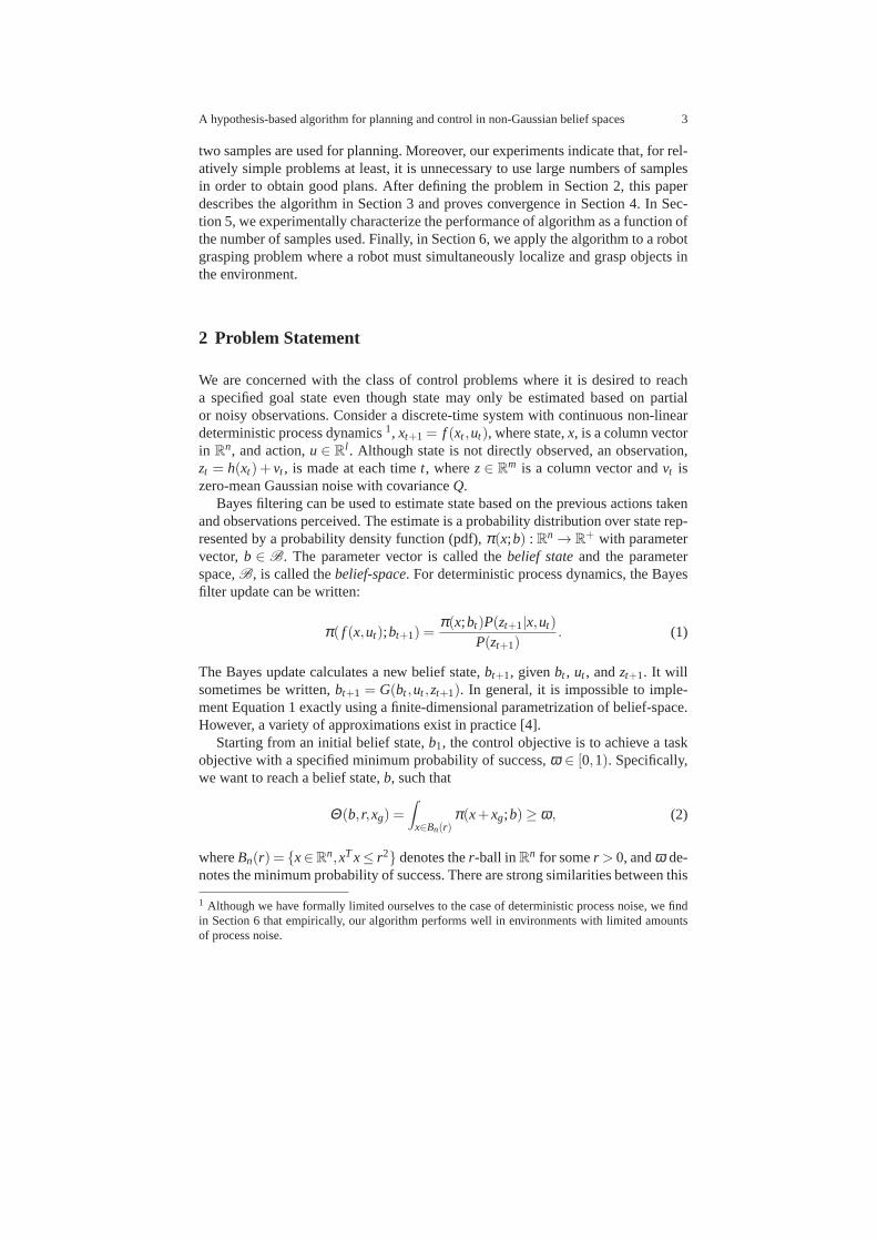
Fig. 2 Illustration of CREATEPLAN . (a) An information-gathering trajectory (state as a functionof time) found using direct transcription. Blue denotes the trajectory that would be obtained if thesystem started in the hypothesis state. Red denotes the trajectory obtained starting in the true state.(b) The planned belief-space trajectory illustrated by probability distributions superimposed overtime. Distributions early in the trajectory are light gray while distributions late in the trajectoryare dark. The seven “X” symbols on the horizontal axis denote thepositions of the samples (reddenotes the true state while cyan denotes the hypothesis). (c) The actual belief-space trajectoryfound during execution. (d-f) Comparison with the EKF-based method proposed in [13]. (d) Theplanned trajectory. (e) The corresponding nominal belief-space trajectory. (f) Actual belief-spacetrajectory.

tical number line in Figure 1. The objective is to localize the vertical end-effectorwith respect to the center of the gap (state) exactly and movethe end-effector tothe center of the gap. The control input to the system is the vertical velocity of theend-effector.

Figure 2(a) illustrates an information-gathering trajectory found by DIRTRAN

that is expected to enable the Bayes filter to determine whether the hypothesis stateis indeed the true state while simultaneously moving the hypothesis to the goal state(end-effector at the center of the gap). The sample set used to calculate the trajec-tory wasx1, . . . ,xk = 5,2,3,4,6,7,8, with the hypothesis sample located atx1 = 5.The action cost used while solving Problem 1 wasα = 0.0085. DIRTRAN was ini-tialized with a random trajectory. The additional small action cost smooths the tra-jectory by pulling it toward shortest paths without changing information gatheringor goal directed behavior much. The trajectory can be understood intuitively. Giventhe problem setup, there are two possible observations: range measurements that“see” one of the two boxes and range measurements that “see” through the gap. Theplan illustrated in Figure 2(a) moves the end effector such that different sequences ofmeasurements would be observed depending upon whether the system were actuallyin the hypothesis state or in another sampled state.


Figures 2(b) and (c) show the nominal belief-space trajectory and the actual tra-jectory, respectively, in terms of a sequence of probability distributions superim-posed on each other over time. Each distribution describes the likelihood that thesystem started out in a particular state given the actions taken and the observationsperceived. The nominal belief-space trajectory in Figure 2(b) is found by simulat-ing the belief-space dynamics forward assuming that futureobservations will begenerated by the hypothesis state. Ultimately, the plannedtrajectory reaches a be-lief state distribution that is peaked about the hypothesisstate,x1 (the red “X”). Incontrast, Figure 2(c) illustrates the actual belief-spacetrajectory found during exe-cution. This trajectory reaches a belief state distribution peaked about the true state(the cyan “X”). Whereas the hypothesis state becomes the maximum of the nominaldistribution in Figure 2(b), notice that it becomes a minimum of the actual distribu-tion in Figure 2(c). This illustrates the main idea of the algorithm. Figure 2(b) can beviewed as a trajectory that “trusts” that the hypothesis is correct and takes actionsthat confirm this hypothesis. Figure 2(c) illustrates that even when the hypothesisis wrong, the distribution necessarily gains information because it “disproves” thehypothesis state (notice the likelihood of the region aboutthe hypothesis is verylow).

Figure 2 (d-f) compares the performance of our approach withthe extendedKalman filter-based (EKF-based) approach proposed in [13].The problem setupis the same in every way except that cost function optimized in this scenario is:

J̄(u1:T−1) =110

(

σ2T

)T σ2T +0.0085uT

1:T−1u1:T−1,

whereσ2T denotes covariance. There are several differences in performance. Notice

that the two approaches generate different trajectories (compare Figures 2(a) and(d)). Essentially, the EKF-based approach maximizes the EKF reduction in varianceby moving the maximum likelihood state toward the edge of thegap where the gra-dient of the measurement function is large. In contrast, ourapproach moves aroundthe state space in order to differentiate the hypothesis from the other samples inregions with a small gradient. Moreover, notice that since the EKF-based approachis constrained to track actual belief state using an EKF Bayes filter, the trackingperformance shown in Figure 2(f) is very bad. The EKF innovation term actuallymakes corrections in the wrong direction. However, in spiteof the large error, theEKF covariance grows small indicating high confidence in theestimate.

4 Analysis

We are interested in the correctness of Algorithm 1. Can we guarantee that Algo-rithm 1 eventually reaches a belief state in the goal region?We show that ifG isan exact implementation of Equation 1, then Algorithm 1 is expected to localizethe true state of the system after a finite number of iterations of the outer loop. Asthe number of iterations of the outer loop goes to infinity, the probability of having

10 Robert Platt, Leslie Kaelbling, Tomas Lozano-Perez, and Russ Tedrake

localized the true system state goes to one. We start by providing a lower bound onthe expected probability of states in a neighborhood of the true state. On a particu-lar iteration of the outerwhile loop in Algorithm 1, suppose that the system beginsin belief state,b1, while the true state isκ , and executes a sequence of actions,u = (u1, . . . ,uT−1) (subscript dropped for conciseness). During execution, the sys-tem perceives observationsz = (z2, . . . ,zT) and ultimately arrives in belief statebT .The probability of a state,y = FT(x,u), estimated by recursively evaluating Equa-tion 1 is:

π(y;bT) = π(x;b1)qx(z,u)p(z,u)

, (10)

whereqx(z,u) = N(z|h(x,u),Q) (11)

is the probability of the observations given that the systemstarts in statex and takesactions,u, and

p(z,u) =∫

x∈Rnπ(x;b1)N(z|h(x,u),Q) (12)

is the marginal probability of the observations givenu. The following Lemma showsthatπ(y;bT) can be lower-bounded in terms of the proximity ofx to the true state,κ .

Lemma 1. Suppose we are given an arbitrary sequence of actions,u, and an arbi-trary initial state, x∈ Rn. Then, the expected probability of y= FT(x,u) found byrecursively evaluating the deterministic Bayes filter update (Equation 1) is

Ez

{

π(y;bT)

π(x;b1)

}

≥ exp(D1(qκ , p)−D1(qκ ,qx)) ,

where qκ , qx, and p are defined in Equations 11 and 12 and D1 denotes the KLdivergence between the arguments.

Proof. The log of the expected change in the probability ofx is:

logEz

{

π(y;bT)

π(x;b1)

}

= logEz

{

qx(z,u)p(z,u)

}

= log∫

z∈Rm

qκ(z,u)qx(z,u)p(z,u)

≥∫

z∈Rmqκ(z)(logqx(z,u)− logp(z,u))

= D1(qκ , p)−D1(qκ ,qx),

where the third line was obtained using Jensen’s inequalityand the last line followsfrom algebra. Taking the exponential gives us the claim.

Lemma 1 expresses the bound in terms of the divergence,D1(qκ , p), with respectto the true state,κ . However, sinceκ is unknown ahead of time, we must find a lowerbound on the divergenceD1(qy, p) for arbitrary values ofy. The following lemma


establishes a bound on this quantity. We use the notation that ‖a‖A =√

aTA−1adenotes the Mahalanobis distance with respect toA.

Lemma 2. Given an arbitraryu and a distribution,ϖ , suppose∃Λ1,Λ2 ⊆ Rn suchthat∀x1,x2∈Λ1×Λ2,‖h(x1,u)−h(x2,u)‖2Q≥ ζ 2 and

∫

x∈Λ1ϖ(x)≥ γ,

∫

x∈Λ2ϖ(x)≥

γ. Then

miny∈Rn

D1(qy, p)≥ 2η2γ2(

1−e−12ζ 2

)2,

whereη = 1/√

(2ϖ)n|Q| is the Gaussian normalization constant.

Proof. By Pinsker’s inequality, we know thatD1(qx, p)≥ 2supz (qx(z,u)− p(z,u))2.

Notice thatp(h(x1,u))≤ η(

1− γ + γe−12ζ 2

)

. Sinceqx(h(x1,u)) = η , we have:

(qx(h(x1,u))− p(h(x1,u)))2≥ γ2

(

1−e−12ζ 2

)2.

We obtain the conclusion by using Pinsker’s inequality.

As a result of Lemmas 1 and 2, we know that we can lower bound theexpectedincrease in probability of a region about the true state by finding regions,Λ1 andΛ2, that satisfy the conditions of Lemma 2 for a givenu. Lemma 3 shows that theseregions exist for anyu with a cost (Equation 3)̄J < 1. The proof uses Lemmas 4and 5, stated and proved in the appendix.

Lemma 3. Suppose thatu is a plan with costJ̄ = J̄(x1, . . . ,xk,u) defined over thesamples, xi , i ∈ [1,k]. If the maximum eigenvalue of the Hessian of h isλ , then∃i ∈ [1,k] such that:

∀r ∈R+,∀δ1,δ2∈Bn(r),‖h(xi+δ1)−h(x1+δ2)‖2Γ (xi ,u)≥[

√

− logJ̄−2(r +cr2)

]

,

where c= λ‖1‖Q/2 and Bn(r) = {x∈ Rn;xTx≤ r2}.

Proof. Considering Equation 3, we know that a cost,J̄, implies that there is at leastone sample,x j , such that

− logJ̄ ≤ Φ(x j ,u)

= ‖h(x j)−h(x1)‖2Γ (x j ,u).

Notice that∀y ∈ Rn, the matrixH(y)TΓ (y,u)−1H(y) is positive semidefinite witheigenvalues no greater than one. Therefore, we know that∀r ∈ R+,δ ∈ Bn(r),

‖H(y)δ‖2Γ (y,u) ≤ r2.

Using Lemma 4 twice to combine the above equations, we have∀r ∈ R+,δ1,δ2 ∈Bn(r),


‖P(x j ,δ1)−P(x1,δ2)‖2Γ (x j ,u) ≥(

√

− logJ̄−2r

)2

,

whereP(x,δ ) = h(x)−H(x)δ . Using Lemma 5, we have that∀x,∈ Rn and δ ∈Bn(r),

‖h(x+δ )−P(x,δ )‖2Γ (x,u) ≤ (cr2)2.

Applying Lemma 4 twice gives us the conclusion of the theorem.

We now state our main theoretical result regarding Algorithm 1 correctness. Twoconditions must be met. First, the planner in step 4 of Algorithm 1 must always findlow-cost plans successfully. Essentially, this guarantees that each plan will acquireuseful information. Second, step 8 of Algorithm 1 must use anexact implementationof the Bayes filter. In practice, we expect that this second condition will rarely bemet. However, our experiments indicate that good results can be obtained usingpractical filter implementations (Section 5).

Theorem 1. Suppose∃r,ε ∈R+ such that∀i ∈ [1,k] and∀δ ∈ Bn(r), π(xi +δ )≥ εwith k≥ 2. Suppose:

1. DIRTRAN (Algorithm 1, step 4) always finds a horizon-T trajectory,u, with cost,

J̄(x1, . . . ,xk,u)≤ exp

[

−(

2r + r2λhλ T−1f ‖1‖Q+

√

logϕ2)2

]

,

whereλh andλ f are the maximum eigenvalues of the Hessian matrix of h and f ,respectively andϕ > 1 is the threshold parameter in step 3 of Algorithm 1; and

2. G is an exact implementation of the Bayesian filter update (Equation 1) in step 8of Algorithm 1.

Then, when Algorithm 1 executes,

1. the expected probability of the true state increases on each iteration of the outerwhile loop by at least2η2γ2(1−1/ϕ), whereη = 1/

√

(2π)n|Q| is the Gaussiannormalization constant,γ = εVoln(r), and Voln(r) is the volume of the r-ball inn dimensions; and

2. as the number of iterations of the outer while loop goes to infinity, the true statebecomes the maximum of the belief state distribution with probability one.

Proof. Condition 2 in the premise implies that√

− logJ̄−2r− r2λhλ τf ‖1‖Q ≥

√

logϕ2.

Lemma 3, gives us that∃i ∈ [1,k] such that∀δ1,δ2 ∈ B(r), ‖h(xi + δ1)− h(x1 +

δ2)‖2Γ (xi ,u) ≥√

logϕ2. Then, Lemma 2 gives us that

miny∈R2

D1(qy, p)≥ 2η2γ (1−1/ϕ)2 ,


whereγ = εVoln(r). Lemma 1 gives us the first conclusion. The constraint thatϕ > 1 implies that the right side of the above equation is positive. As a result, theprobability of the true state is expected to increase on eachiteration of the outerwhile loop and we have the second conclusion.

At the end of Section 3.1, we noted that the planning problem solved in step 4of Algorithm 1 was linear in the dimensionality of the underlying space. Theorem 1asserts that the algorithm is correct with as few as two samples. As a result, we knowthat the linear constant can be as small as two.

5 Experiments

laserarm

(a)

−2 0 2 4 6

−2

−1

0

1

2

3

4

5

(b)

0 100 200 300 400 500 600 7004

5

6

7

8

9

10

11

12

Time step

Ent

ropy

(c)

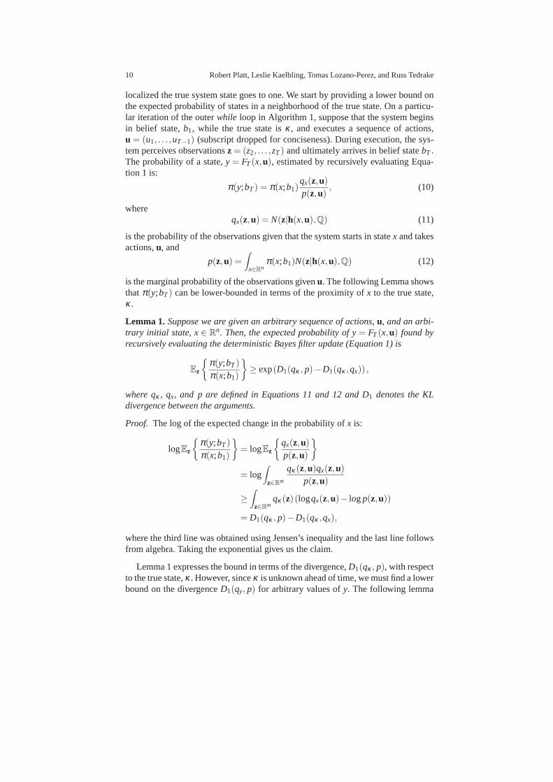
Fig. 3 (a) the experimental scenario. (b) a path found by Algorithm 1 with a nine-sample planner.It starts in the upper right and ends at a point directly in front of the right-most box. The red circlesdenote where re-planning occurred. (c) belief state entropyas a function of time step. The solidblack line corresponds to the trajectory shown in (b). The dashed blue lines correspond to fiveadditional nine-sample runs.

From a practical perspective, the preceding analysis is useful because it tellsus that if we execute thewhile loop in Algorithm 1 a sufficient number of times,we can expect to localize the state of the system with arbitrary accuracy (we candrive Θ(b, r,xg) arbitrarily low). However, for this result to hold, we require theplanner to find low cost paths each time it is called and for thetracking Bayesfilter to be an exact realization of Equation 1 (the premise ofTheorem 1). Sincethese conditions are difficult to meet in practice, an important question is how wellthe approach works for approximately accurate Bayes filter implementations andfor planners that only succeed some of the time. Furthermore, we are interested inknowing how the performance of the algorithm changes with the number of samplesused to parametrized the planner. Figure 3(a) illustrates the experimental scenario.A two-link robot arm moves a hand in the plane. A single range-finding laser ismounted at the center of the hand. The laser measures the range from the end-effector to whatever object it “sees”. The hand and laser areconstrained to remain


horizontal. The position of the hand is assumed to be measured perfectly. Thereare two boxes of known size but unknown position to the left ofthe robot (fourdimensions of unobserved state). The boxes are constrainedto be aligned with thecoordinate frame (they cannot rotate). The control input tothe system is the planarvelocity of the end-effector. The objective is for the robotto localize the two boxesusing its laser and move the end-effector to a point directlyin front of the right-mostbox (the box with the largestx-coordinate) so that it can grasp by extending andclosing the gripper. On each time step, the algorithm specified the real-valued two-dimensional hand velocity and perceived the laser range measurement. If the lasermissed both boxes, a zero measurement was perceived. The (scalar) measurementswere corrupted by zero-mean Gaussian noise with 0.31 standard deviation.

−2 −1 0 1 2−2

−1.5

−1

−0.5

0

0.5

1

1.5

2

X axis

Y a

xis

(a)

−2 −1 0 1 2−2

−1.5

−1

−0.5

0

0.5

1

1.5

2

X axis

Y a

xis

(b)

−2 −1 0 1 2−2

−1.5

−1

−0.5

0

0.5

1

1.5

2

X axisY

axi

s

(c)

−2 −1 0 1 2−2

−1.5

−1

−0.5

0

0.5

1

1.5

2

X axis

Y a

xis

(d)

−4 −3 −2 −1 0 1 2

−2

−1

0

1

2

3

X axis

Y a

xis

(e)

−4 −3 −2 −1 0 1 2−3

−2

−1

0

1

2

X axis

Y a

xis

(f)

−4 −3 −2 −1 0 1 2

−2

−1

0

1

2

3

X axis

Y a

xis

(g)

−4 −3 −2 −1 0 1 2

−2

−1

0

1

2

3

X axis

Y a

xis

(h)

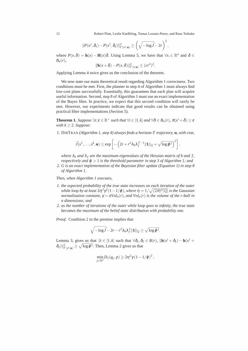
Fig. 4 Histogram probability distributions (a-d) and planner sample sets (e-h) at time steps 10,100, 200, and 300 during the path shown in Figure 3(b).

Figure 3(b) illustrates the path of the hand (a point directly between the twojaws of the gripper) found by running our algorithm parametrized by nine samples.The state space was four dimensional and comprised of two boxlocations rang-ing between[−1,1] on thex-axis and[−2,2] on they-axis. The hand starts in theupper right corner at(5,5) and ends at a point directly in front of the lower rightbox. The blue line shows the path and the red circles identifythe points along thepath at which re-planning occurred (there are 14 re-plan events in this example).The tracking Bayes filter was implemented using a gridded histogram filter com-prised of 62500 bins over the four-dimensional space (the position of each of thetwo boxes was denoted by a point in a 10×25 grid). At the start of planning, theprior histogram distribution was assumed to be uniform. Thecost function opti-mized by the DIRTRAN planner (Equation 6) was parametrized byα = 0.01 andV = diag(0.5) (Equations 3 and 4). The planning horizon wasT = 50. The algo-rithm did not terminate until the histogram Bayes filter was 90% confident that ithad localized the right-most box to within±0.3 of its true location (ω = 0.9 in step


1 of Algorithm 1). Figure 4(a)-(d) show snapshots of the histogram distribution attime steps 10, 100, 200, and 300. (This is actually a two-dimensional projection ofthe four dimensional distribution illustrating the distribution over the location ofonebox only.) Figure 4(e)-(h) show the nine samples used to parametrize the planningalgorithm at the four snapshots. Initially, (in Figures 4 (a) and (e), the distributionis high-entropy and the samples are scattered through the space. As time increases,the distribution becomes more peaked and the sample sets become more focused.The solid black line in Figure 3(b) shows the entropy of the histogram distributionas a function of time step. As expected, entropy decreases significantly over the tra-jectory. For comparison, the five additional blue dotted lines in Figure 3(c) showentropy results from five additional identical experiments. Note the relatively smallvariance amongst trajectories. Even though the algorithm finds a very different tra-jectory on each of these runs, performance is similar. Theseresults help answer twoof the questions identified at the beginning of the section. First, Figure 4 suggeststhat in at least one case, the histogram filter was adequate torepresent the belief statein the context of this algorithm even though it is a coarsely discretized approxima-tion to the true distribution. The black line in Figure 3(c) suggests that DIRTRAN

was an effective tool for planning in this scenario. The six additional runs illustratedin Figure 3(c) indicate that these results are typical.

0 200 400 600 800 10004

5

6

7

8

9

10

11

12

Time step

Ent

ropy

(a)

0 200 400 600 800 10004

5

6

7

8

9

10

11

12

Time step

Ent

ropy

(b)

−2 0 2 4 6

−2

−1

0

1

2

3

4

5

(c)

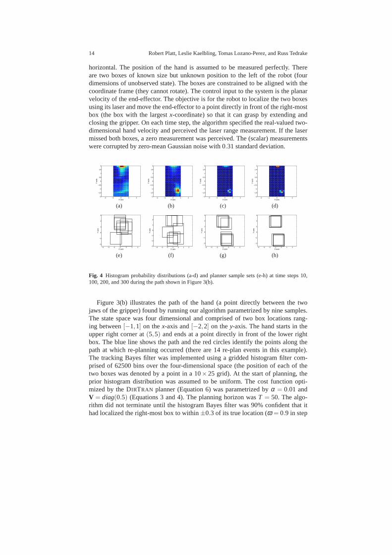
Fig. 5 (a) comparison of entropy averaged over six runs for four different planner sample setsizes (36 samples, solid black line; 9 samples, dashed blue line; 4 samples, dotted magenta line; 2samples, dash-dot green line). (b) comparison of the six thirty-six-sample runs (solid black) withthe six two-sample runs (dashed blue). (c) a path found using a two-sample planner.

The other question to be answered concerns the effect of the number of sampleson algorithm performance. To find an answer, we have run the algorithm in the sce-nario described above for four contingencies where the planner was parametrized bytwo, four, nine, and thirty-six samples. Figure 5(a) compares the average (over sixruns each) information-gathering performance for the fourcontingencies. Althoughincreasing the number of samples improves algorithm performance, the gains di-minish as the number of samples increases. Figure 5(b) compares the two-sampleruns with the thirty-six-sample runs and demonstrates thatthe improvement is sta-tistically significant. The comparison of Figure 5(c) with Figure 3(b) suggests that(in this experiment, at least) the trajectories produced bythe high-sample plannerare better than those produced by the low-sample planner because the high-sample


planner does a better job covering the space in front of the boxes. These results showthat it is valuable to expend computational effort planningan information-gatheringtrajectory, even in this simple example. The results also show that the performanceof our algorithm smoothly degrades or improves with fewer ormore samples usedduring planning. Even with the minimum of two samples, the algorithm is capableof making progress.

6 Robot Grasping application

We apply our approach to an instance of the robot grasping problem where it isnecessary to localize and grasp a box. We refer to this version of the problem, whereperception is incorporated into the problem statement, as “simultaneous localizationand grasping” (SLAG). Two boxes of unknown dimensions are presented to therobot. The objective is to localize and grasp the box which isinitially found directlyin front of the left paddle. This is challenging because the placement of the twoboxes may make localization of the exact position and dimensions of the boxesdifficult.

6.1 Problem setup

(a) (b) (c)

Fig. 6 Illustration of the grasping problem, (a). The robot must localize the pose and dimensionsof the boxes using the laser scanner mounted on the left wrist. Thisis relatively easy when theboxes are separated as in (b) but hard when the boxes are pressed together as in (c).

Our robot,Paddles, has two arms with one paddle at the end of each arm (seeFigure 6(a)). Paddles may grasp a box by squeezing the box between the two pad-dles and lifting. We assume that the robot is equipped with a pre-programmed “lift”function that can be activated once the robot has placed its two paddles in opposi-tion around the target box. Paddles may localize objects in the world using a laserscanner mounted to the wrist of its left arm. The laser scanner produces range datain a plane parallel to the tabletop over a 60 degree field of view.


−0.4−0.200.20.4

−0.2

−0.1

0

0.1

0.2

0.3

0.4

x (meters)

y (m

eter

s)

(a)

−0.4−0.200.20.4

−0.2

−0.1

0

0.1

0.2

0.3

0.4

x (meters)

y (m

eter

s)

(b)

−0.4−0.200.20.4

−0.2

−0.1

0

0.1

0.2

0.3

0.4

x (meters)

y (m

eter

s)

(c)

(d) (e) (f)

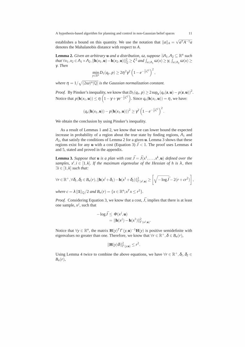
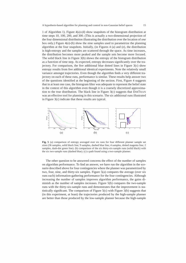
Fig. 7 Example of a box localization task. In (a) and (d), the robot believes the gap between theboxes is large and plans to localize the boxes by scanning thisgap. In (b) and (e), the robot hasrecognized that the boxes abut each other and creates a plan to increase gap width by pushing theright box. In (c) and (f), the robot localizes the boxes by scanning the newly created gap.

We use Algorithm 1 to localize the planar pose of the two boxesparametrizedby a six-dimensional underlying metric space. The boxes areassumed to have beenplaced at a known height. We reduce the dimensionality of theplanning problemby introducing an initial perception step that localizes the depth and orientation ofthe right box using RANSAC [7]. From a practical perspective, this is a reasonablesimplification because RANSAC is well-suited to finding the depth and orientationof a box that is assumed to be found in a known region of the laser scan. The remain-ing (four) dimensions that are not localized using RANSAC describe the horizontaldimension of the right box location and the three-dimensional pose of the left box.These dimensions are localized using a Bayes filter that updates a histogram distri-bution over the four-dimensional state space based on lasermeasurements and armmotions measured relative to the robot. The histogram filteris comprised of 20000bins: 20 bins (1.2 cm each) describing right box horizontal position times 10bins(2.4 cm each) describing left box horizontal position times 10 bins (2.4 cm each)describing left box vertical position times 10 bins (0.036 radians each) describingleft box orientation. While it is relatively easy for the histogram filter to localize theremaining four dimensions when the two boxes are separated by a gap (Figure 6(b)),notice that this is more difficult when the boxes are pressed together (Figure 6(c)).In this configuration, the laser scans lie on the surfaces of the two boxes such that itis difficult to determine where one box ends and the next begins. Note that it is diffi-cult to locate the edge between abutting boxes reliably using vision or other sensormodalities – in general this is a hard problem.


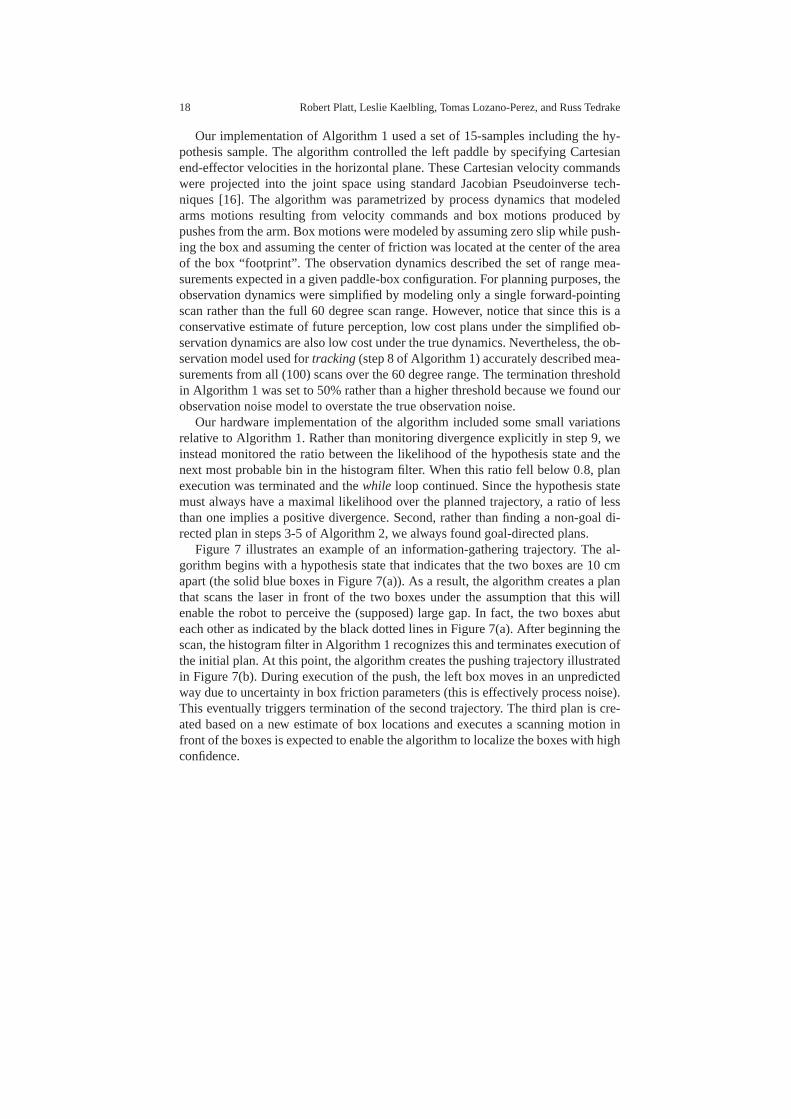
Our implementation of Algorithm 1 used a set of 15-samples including the hy-pothesis sample. The algorithm controlled the left paddle by specifying Cartesianend-effector velocities in the horizontal plane. These Cartesian velocity commandswere projected into the joint space using standard JacobianPseudoinverse tech-niques [16]. The algorithm was parametrized by process dynamics that modeledarms motions resulting from velocity commands and box motions produced bypushes from the arm. Box motions were modeled by assuming zero slip while push-ing the box and assuming the center of friction was located atthe center of the areaof the box “footprint”. The observation dynamics describedthe set of range mea-surements expected in a given paddle-box configuration. Forplanning purposes, theobservation dynamics were simplified by modeling only a single forward-pointingscan rather than the full 60 degree scan range. However, notice that since this is aconservative estimate of future perception, low cost plansunder the simplified ob-servation dynamics are also low cost under the true dynamics. Nevertheless, the ob-servation model used fortracking(step 8 of Algorithm 1) accurately described mea-surements from all (100) scans over the 60 degree range. The termination thresholdin Algorithm 1 was set to 50% rather than a higher threshold because we found ourobservation noise model to overstate the true observation noise.

Our hardware implementation of the algorithm included somesmall variationsrelative to Algorithm 1. Rather than monitoring divergenceexplicitly in step 9, weinstead monitored the ratio between the likelihood of the hypothesis state and thenext most probable bin in the histogram filter. When this ratiofell below 0.8, planexecution was terminated and thewhile loop continued. Since the hypothesis statemust always have a maximal likelihood over the planned trajectory, a ratio of lessthan one implies a positive divergence. Second, rather thanfinding a non-goal di-rected plan in steps 3-5 of Algorithm 2, we always found goal-directed plans.

Figure 7 illustrates an example of an information-gathering trajectory. The al-gorithm begins with a hypothesis state that indicates that the two boxes are 10 cmapart (the solid blue boxes in Figure 7(a)). As a result, the algorithm creates a planthat scans the laser in front of the two boxes under the assumption that this willenable the robot to perceive the (supposed) large gap. In fact, the two boxes abuteach other as indicated by the black dotted lines in Figure 7(a). After beginning thescan, the histogram filter in Algorithm 1 recognizes this andterminates execution ofthe initial plan. At this point, the algorithm creates the pushing trajectory illustratedin Figure 7(b). During execution of the push, the left box moves in an unpredictedway due to uncertainty in box friction parameters (this is effectively process noise).This eventually triggers termination of the second trajectory. The third plan is cre-ated based on a new estimate of box locations and executes a scanning motion infront of the boxes is expected to enable the algorithm to localize the boxes with highconfidence.


(a) (b)

0 50 100 150 2000

0.05

0.1

0.15

0.2

0.25

Filter update number

Loca

lizat

ion

erro

r (m

eter

s)

(c)

0 50 100 150 2000

0.05

0.1

0.15

0.2

0.25

Filter update number

Loca

lizat

ion

erro

r (m

eter

s)(d)

Fig. 8 “Easy” and “hard” experimental contingencies. (a) shows images of the 12 randomly se-lected “easy” configurations (both box configurations chosen randomly) superimposed on eachother. (b) shows images of the 12 randomly selected “hard” configurations (boxes abutting eachother). (c) and (d) are plots of error between the maximum a posteriori localization estimate andthe true box pose. Each line denotes a single trial. The red “X” marks denote localization error atalgorithm termination.

6.2 Localization Performance

At a high level, the objective of SLAG is to robustly localizeand grasp objects evenwhen the pose or shape of those objects is uncertain. We performed a series of ex-periments to evaluate how well this approach performs when used to localize boxesthat are placed in initially uncertain locations. On each grasp trial, the boxes wereplaced in a uniformly random configuration (visualized in Figures 8(a) and (c)).There were two experimental contingencies: “easy” and “hard”. In the easy contin-gency, both boxes were placed randomly such that they were potentially separatedby a gap. The right box was randomly placed in a 13×16 cm region over a rangeof 15 degrees. The left box was placed uniformly randomly in a20×20 cm regionover 20 degrees measured with respect to the right box (Figure 8(a)). In the hardcontingency, the two boxes were pressed against each other and the pair was placedrandomly in a 13×16 cm region over a range of 15 degrees (Figure 8(b)).

Figures 8(c) and (d) show right box localization error as a function of the num-ber of updates to the histogram filter since the trial start. 12 trials were performedin each contingency. Each blue line denotes the progress of asingle trial. The ter-mination of each trial is indicated by the red “X” marks. Eacherror trajectory is


referenced to the ground truth error by measuring the distance between the final po-sition of the paddle tip and its goal position in the left corner of the right box usinga ruler. There are two results of which to take note. First, all trials terminate withless than 2 cm of error. Some of this error is a result of the coarse discretizationof possible right box positions in the histogram filter (notealso the discreteness ofthe error plots). Since the right box position bin size in thehistogram filter is 1.2cm, we would expect a maximum error of at least 1.2 cm. The remaining error isassumed to be caused by errors in the range sensor or the observation model. Sec-ond, notice that localization occurs much more quickly (generally in less than 100filter updates) and accurately in the easy contingency, whenthe boxes are initiallyseparated by a gap that the filter may used to localize. In contrast, accurate local-ization takes longer (generally between 100 and 200 filter updates) during the hardcontingency experiments. Also error prior to accurate localization is much largerreflecting the significant possibility of error when the boxes are initially placed inthe abutting configuration. The key result to notice is that even though localizationmay be difficult and errors large during a “hard” contingency, all trials ended witha small localization error. This suggests that our algorithm termination conditionin step 1 of Algorithm 1 was sufficiently conservative. Also notice that the algo-rithm was capable of robustly generating information gathering trajectories in all ofthe randomly generated configurations during the “hard” contingencies. Without thebox pushing trajectories found by the algorithm, it is likely that some of the hardcontingency trials would have ended with larger localization errors.

7 Discussion

Creating robots that can function robustly in unstructuredenvironments has alwaysbeen a central objective of robotics. In order to achieve this, it is necessary to de-velop algorithms capable of actively localizing the state of the world while alsoreaching task objectives. We introduce an algorithm that achieves this by planning inbelief-space, the space of probability distributions overthe underlying state space.Crucially, our approach is capable of reasoning about trajectories through a non-Gaussian belief-space. The fact that we can plan effectively non-Gaussian beliefspaces makes our algorithm different than most other beliefspace planning algo-rithms currently in the literature. The non-Gaussian aspect is essential because inmany robot problems it is not possible to track belief state accurately by project-ing onto an assumed Gaussian density function (this is the case, for example, in thetwo-box example described in this paper). This paper provides a novel sufficientcondition for guaranteeing that the probability of the truestate found by the Bayesfilter increases (Lemma 1). We show that our algorithm meets these conditions and,as a result, converges to the true state with probability one(Theorem 1). Althoughour theoretical results hold only under strict conditions,our experiments indicatethat the algorithm performs well in practice. We empirically characterize the effectof changing the number of samples used to parametrize the algorithm on the result-


ing solution quality. We find that algorithm performance is nearly optimized usingvery few (between two and nine) samples and that, as a result,the planning step inour algorithm is computationally efficient. Finally, we illustrate our approach in thecontext of a robot grasping problem where a robot must simultaneously localize andgrasp and object that is known only to be found somewhere in front of the robot.

References

1. Y. Bar-Shalom. Stochastic dynamic programming: Caution and probing. IEEE Transactionson Automatic Control, pages 1184–1195, October 1981.

2. D. Bayard and A. Schumitzky. Implicit dual control based on particle filtering and forwarddynamic programming.Int’l Journal of Adaptive Control and Signal Processing, 24(3):155–177, 2010.

3. J. Betts.Practical methods for optimal control using nonlinear programming. Siam, 2001.4. A. Doucet, N. Freitas, and N. Gordon, editors.Sequential monte carlo methods in practice.

Springer, 2001.5. N. Du Toit and J. Burdick. Robotic motion planning in dynamic,cluttered, uncertain environ-

ments. InIEEE Int’l Conf. on Robotics and Automation (ICRA), 2010.6. T. Erez and W. Smart. A scalable method for solving high-dimensional continuous POMDPs

using local approximation. InProceedings of the International Conference on Uncertainty inArtificial Intelligence, 2010.

7. M. Fischler and R. Bolles. Random sample consensus: A paradigm formodel fitting withapplications to image analysis and automated cartography.Communications of the ACM,24:381–395, 1981.

8. D. Jacobson and D. Mayne.Differential dynamic programming. Elsevier, 1970.9. H. Kurniawati, D. Hsu, and W. S. Lee. SARSOP: Efficient point-based POMDP planning by

approximating optimally reachable belief spaces. InProceedings of Robotics: Science andSystems (RSS), 2008.

10. S. LaValle and J. Kuffner. Randomized kinodynamic planning. International Journal ofRobotics Research, 20(5):378–400, 2001.

11. S. Miller, A. Harris, and E. Chong. Coordinated guidance of autonomous uavs via nominalbelief-state optimization. InAmerican Control Conference, pages 2811–2818, 2009.

12. C. Papadimitriou and J. Tsitsiklis. The complexity of Markov decision processes.Mathemat-ics of Operations Research, 12(3):441–450, 1987.

13. R. Platt, R. Tedrake, L. Kaelbling, and T. Lozano-Perez.Belief space planning assumingmaximum likelihood observations. InProceedings of Robotics: Science and Systems (RSS),2010.

14. S. Prentice and N. Roy. The belief roadmap: Efficient planning in linear POMDPs by factoringthe covariance. In12th International Symposium of Robotics Research, 2008.

15. S. Ross, J. Pineau, S. Paquet, and B. Chaib-draa. Online planning algorithms for POMDPs.The Journal of Machine Learning Research, 32:663–704, 2008.

16. L. Sciavicco and B. Siciliano.Modelling and Control of Robot Manipulators. Springer, 2000.17. T. Smith and R. Simmons. Point-based POMDP algorithms: Improved analysis and imple-

mentation. InProc. Uncertainty in Artificial Intelligence, 2005.18. J. Van der Berg, P. Abbeel, and K. Goldberg. LQG-MP: Optimized path planning for robots

with motion uncertainty and imperfect state information. InProceedings of Robotics: Scienceand Systems (RSS), 2010.


Appendix

Lemma 4. If ‖x‖2A ≥ θ 2, ‖δ‖2A ≤ ε2, andθ ≥ ε, then‖x− δ‖2A ≥ (θ − ε)2, wherex,δ ∈ Rn, θ ,ε ∈ R+, and A= AT ≥ 0,

Proof. By the triangle inequality, we have‖x‖A ≤ ‖δ‖A+ ‖x− δ‖A. Rearranging,this becomes‖x− δ‖A ≥ ‖x‖A−‖δ‖A. We obtain the conclusion by squaring bothsides and substitutingθ andε.

Lemma 5. If f(x) = ( f1(x), . . . , fn(x))T is a vector-valued function with Jacobian

matrix F, and each scalar-valued component, fi , has a Hessian matrix with a max-imum eigenvalue ofλ f , then∀x∈X ,δ ∈ Bn(r),

‖ f (x+δ )−P(x,δ )‖2A≤r4λ 2

f

4‖1‖2A,

where1 is a column vector of n ones, P(x,δ ) = f (x) + F(x)δ is the first-orderTaylor expansion off, λA is the maximum eigenvalue of A, and Bn(r) is the r-ball indimension n.

Proof. For all i ∈ [1,n], the Taylor remainder isRi(x,δ ) = f (x+δ )−P(x,δ ). By theTaylor remainder theorem, we know that|Ri(x,δ )| ≤ 1

2δ TCiδ , whereCi is the Hes-sian of fi . Notice that∀δ ∈Bn(r), δ TCiδ ≤ r2λ f . LetR(x,δ )= (R1(x,δ ), . . .Rn(x,δ ))T .

Then‖R(x,δ )‖2A≤r4λ 2

f4 ‖1‖2A and we have the conclusion.

Date post:	16-Feb-2022
Category:	Documents
Upload:	others
View:	1 times
Download:	0 times

A hypothesis-based algorithm for planning and control in ...

Documents