› img › doi › 0013-3264 › 2007 › 0013-32640773007S.pdf MOnOpSOny In thE LAbOr MArKEt:...

�

JEL Classification Numbers: J42, L21, D60,

ORIGINALNI NAUČNI RADOVI / SCIENTIFIC PAPERS

Đorđe Šuvaković Olgin and DOI:10.2298/EKA0773007S Goran Radosavljević*

MOnOpSOny In thE LAbOr MArKEt: prOfIt vS. WAgE MAxIMIzAtIOn**

MOnOpSOn nA trŽIŠtU rADA: MAKSIMIrAnJE prOfItA prEMA MAKSIMIrAnJU pLAtA

AbStrACt: This paper compares the effi-ciency of profit- and wage-maximizing (PM and WM) monopsony in the labor market. We show that, both locally and globally, a PM monopsony may well be dominated by its WM twin, where the local and global dominance are defined with respect to a single (inverse) labor supply function and a single family of such functions. This fam-ily is always divided in the two disjoint (sub)families of the PM and WM domi-nance. We also analyze some major factors that explain the size of these (sub)families.

KEy WOrDS: Monopsony; Labor Market; Profit Maximization; Wage Maximization

ApStrAKt: U ovom radu se poredi efi-kasnost monopsona na tržištu rada. Pos-matraju se dva slučaja: monopson koji maksimizira profit (PM) i monopson koji maksimizira nadnice (WM). Pokazano je da WM monopson može da dominira, lo-kalno i globalno, nad PM monopsonom, pri čemu su lokalna i globalna dominacija definisane uzimajući u obzir jednu (inver-znu) funkciju ponude rada i familiju takvih funkcija. Ta familija je uvek podeljena na dve disjunktne (pod)familije, tako da u ok-viru jedne (pod)familije dominira PM, a u okviru druge WM monopson. Analiziraju se i glavni faktori koji utiču na veličinu tih (pod)familija.

KLJUČnE rEČI: monopson, tržište rada, maksimizacija profita, maksimizacija nadnice

* Foundation for the Advancement of Economics, Belgrade** This research was supported by a grant from CERGE-EI Foundation under a program of the

Global Development Network (GDN). All opinions expressed are those of the author and have not been endorsed by CERGE-EI or the GDN. We thank Mario Ferrero, Alan Kirman, Hugh Neary, Pavle Petrovic, and Jan Svejnar for helpful comments and/or suggestions. The usual disclaimer applies.

1. Introduction

After a period of neglect, monopsony in the labor market seems to be regaining its place, both in the labor and industrial economics1.

Thus, recent contributions focus either on the empirical relevance of monopsonistic behavior (Boal and Ransom, 1997; Manning, 2003a; 2003b; Staiger et al, 1999) or on theoretical explanations of the emergence of such behavior (Bhaskar et al, 2004; Boal and Ransom, 1997; Manning, 2003a; 2003b).

Our emphasis is different. We take for granted the existence of monopsonistic labor markets but concentrate on their comparative efficiency due to supposedly different objectives of firms that operate on such markets.

It is normally assumed that monopsonistic enterprises act as profit maximizers. The purpose of this paper is to examine the impact of wage-maximizing (WM) behavior - frequently analyzed in the corresponding literature2 - on the efficiency of monopsonistic labor markets, as well as to compare this efficiency with that of labor markets populated with profit-maximizing firms (PMFs).

In this connection it should be emphasized that WM firms (WMFs) are most often identified with the Western type producer cooperatives and partnerships in the service sector (see, for example, Dreze, 1989; Pencavel and Craig, 1994).

Recently, such enterprises have also been linked with the many insider-controlled firms that have emerged during the privatization process in the post-socialist countries (Blanchard, 1997; IBRD, 1996; Roland, 2000).

In a sense, the present paper follows on from Domar’s (1966) early analysis of a WM monopsony in the labor market. However, unlike Domar, we restrict ourselves to a systematic comparison of the efficiency of monopsonistic WMF and PMF, when they operate in the labor market.

1 Valuable recent sources that assess the relevance of the non-wage-taking phenomenon are Boal and Ransom (1997; 2002) and Manning (2003a; 2003b).

2 The comprehensive survey of the vast literature on WM firms is Bonin and Putterman (1987). For a concise review see Bonin, Jones and Putterman (1993).

�

Đorđe Šuvaković Olgin and Goran Radosavljević

The structure of the paper is as follows.

In Section 1 of Part II, we first define a typical family of increasing (inverse) labor supply or wage functions, which enable both PMF and WMF to earn nonnegative profit under convex technology.

To motivate the reader, we then give a graphic illustration of this family to focus, in Section 2 of Part II, on the member of the family of wage functions that yields exactly the Pareto optimal equilibrium of a no loss making WMF. Such a function always exists. This also means that in the case considered a WM monopsony Pareto dominates its PM twin, since the latter - apart from the case of perfect wage discrimination - can never reach the Paretian norm.

In Part III we represent the PM monopsony equilibrium in the form appropriate for straightforward efficiency comparisons. Then, we formally characterize the two types of WM monopsony equilibrium, evoked by Domar (1966).

In Part IV we show that the family of wage functions, defined in part II, is always divided, by some neutral member-function, into an upper and a lower subfamily, where the former ensures the dominance of a WMF over PMF, while within the latter the converse is true.

In Part V we discuss the results of systematic numerical simulations, performed to get an insight into the relative size of the WMF and PMF dominance regions as well as into the sensitivity of this size to the shape of labor’s marginal product curve, the curvature of labor supply functions, and the level of the entry wage. In Appendix, we graphically present the three arguably most representative exercises, which test the sensitivity of the WMF/PMF dominance relation to the degree of curvature of the labor supply functions, in the “neutral” case of linear marginal product of labor.

Summary and concluding remarks, where the latter also address the issue of how to privatize a non-wage-taking firm, are left for Part VI.

Monopsony in the Labor Market

�

2. A Typical Family of Wage Functions and the Case When a WM Monopsony Pareto Dominates its PM Twin

2.1. The S family of inverse labor supply or wage functions

In order to define the particular one-parameter family of inverse labor supply or wage functions that we consider and which yields nonnegative profit for a non-wage-taking firm, we first introduce the function of firm’s (non-capital) income per unit of labor or a ‘full’ wage, y:

LCLXy −= )(

(1)

where X(L) and L are the short-run production function and the labor input respectively, and where, by suitably choosing the measure of X, its (constant) price, p, is normalized to unity. Finally, C stands for fixed (capital) costs.

The reader familiar with the theory of a WMF - see, for example, Dreze (1989), Bonin and Putterman (1987) - will recognize in (1) the objective function of such an enterprise. Here, the y function - depicted in Figures 1 and 2 below - will, inter alia, serve to define the steepest wage curve that yields zero profit both to a WM and conventional PM firm.

In the monopsonistic labor market a typical (inverse) labor supply or wage function faced by a firm may be represented as:

Wk = f(L, ak) ≡ Wk(L) , L > 0 , (2)

where Wk is a wage rate or a supply price of labor, L is a firm’s demand for labor or potential labor supply and ak is (nonnegative) parameter, which represents a measure of labor scarcity experienced by a firm.

In what follows ak will be (discretely) varied so as to cover all relevant degrees of labor scarcity - see relation (3) and the ensuing relations (4) - (5a).

The f function is further characterized as follows:

10


0>′≡∂∂ fLf

(2a)

02

2

≥′′≡∂∂ fLf

(2b)

0>≡∂∂

kak

faf

(2c)

0>′≡∂

′∂ka

k

faf

(2d)

While the interpretation of (2a)-(2c) in straightforward, (2d) assumes that an increase in labor scarcity leads to a greater increase in the wage rate, given any (infinitesimal) increase in the demand for labor.

By varying the ak parameter within the interval defined in (3) below, we obtain the one-parameter family of Wk functions, denoted by S:

S = {Wk = f(L, ak) ≡ Wk(L) , ak ∈ (ae, az)} , (3)

where the S family is bounded from below by the horizontal entry-wage schedule We , depicted in Figure 13,

We = f(L, ae) = const > 0 (4)

In (4) the ae value of ak generates the equilibrium labor use, Le , by a wage taking PMF:

Le = arg [X’(L) – f(L, ae) = 0], |ea∀ f(L, ae) = const > 0 (4a)

3 Note that in Figure 1, as in most of the numerical simulations of part V, we assume, for simplicity, that the entry-wage is insensitive to the value of the ak parameter.


11

On the other hand, the upper boundary of S reduces to the function Wz = f(L, az), which simultaneously satisfies the following two conditions, i.e., defines the function that has the tangency point with y=y(L):

Wz (L) ≡ f(L, az) = y(L) , Wz’ (L)

LaLf z

∂∂≡ ),(

= y’(L) (5)

In (5), L = Lz represents the corresponding equilibrium employment, implied by az, which, following eq. (5), satisfies:

Lz = arg[Wz’ (L) - y’(L) = 0] , Lz = arg[Wz (L) - y(L) = 0] (5a)

Thus, as already stated, eq. (4) defines the hypothetical case of a wage-taking enterprise - i.e., of zero labor scarcity faced by a single firm - while relation (5) defines the steepest relevant wage function which, by definition, yields zero profit both to a PMF and WMF - see the Wz curve of Figure 1.

Figure 1. The S family of wage functions of (3), represented by the shaded area bordered by the horizontal line We of (4) and the steepest relevant wage curve, Wz , of (5).

0 3

2

X’ y

Wz

We

LLz L

E

Mm

Lm

Z

We

e

N

X’0

12


- Mm = Wm + LW’m is marginal cost of monopsonistic labor, obtained from the wage function Wm , displayed below, and depicted in Figure 2;

- the functions y and X’ are those of (1) and (7); - Lz and Le are respectively from (5a) and (4a), while the PMF labor use may be written as Lm

Π = arg max [Π(L) ≡ X(L) – LWk(L) – C], cf. eq. (7a);

Figure 1 is obtained using the following parameter forms:

- X’ = 3.5-0.6L2, C = 2.85, y = 3.5 - 0.2L2 - C/L, We = 0.4, Wn = 0.4 + 0.0803L2, Wm

= 0.4 + 0.237L2, Wz = 0.4 + 0.344L2, Mm = 0.4 + 0.711L2

Note finally that, when coupled with the inequality L > 0 of (2), eqs. (2a)-(2d), which describe one well-behaved (inverse) labor supply or wage function, also ensure that any two member-functions of the S family do not have any common point. Among other things, this means that any member-function divides S in the two disjoint subfamilies.

2.2 The Pareto dominance of a WM monopsony over its PM twin: The graphical example

As we said, in this section we provide a particular numerically generated example in which a WM monopsony achieves exactly the Pareto optimum and thus, by definition, Pareto dominates its PM twin, since the latter, except in the case of perfect wage discrimination, can never reach the Paretian norm.

When labor is the only variable input, the WMF maximand of income-per-worker, y, is defined as in eq. (1) above.

At the same time, the unconstrained maximum of y in L is defined by the well-known WMF equilibrium condition, X’(L) = y(L) , displayed in relation (14) below, where X’(L) and y(L) are, respectively, labor’s marginal product and income-per-labor-unit functions, and where the product price, p, is taken to be the numeraire, p = 1.

Suppose now that one family-member wage function - denoted by Wm(L), defined in eq. (12), and depicted in Figure 2 – intersects the y(L) function of eq.

(1) just at its maximum, ymL , of eq. (12a).


13

In this case, we will have:

Wm(L) = X’ (5b)

Thus, for the Wm(L) wage function, the WM monopsony equilibrium, Lym,

coincides with the Pareto optimum, LyP - see also Figure 2. Hence, by definition,

a WMF Pareto dominates PMF, and, in the case considered, a WMF produces (about) 12% more output than its PMF twin.

3. The Equilibrium of a PM and WM Monopsony: A general comparison

3.1. The two forms of the PM monopsony equilibrium

Starting from (2), the economic profit of the PM monopsony, Π may be represented as:

Π = X(L) – LWk(L) – C , (6)

where X(L) and C appear in (1).

The standard first order condition for the maximum of Π in L reads:

X’(L) – [Wk(L) + LW’k(L)] = 0 , (7)

where X’ and ( )fWk ′≡′ respectively denote the first derivatives of X and Wk with respect to L, and where, from (6), the value of L which achieves the maximum of Π may be written as:

LΠ = arg max [Π(L) ≡ X(L) – LWk(L) – C] (7a)

The standard PM monopsony equilibrium condition, obtained from (7), reads:

X’(L) = Wk(L) + LW’k(L) ≡ Mk(L) , (8)

where the R.H.S. of eq. (8) is the marginal labor cost of a PM monopsony, denoted by Mk(L).

14


To simplify the efficiency comparison - which will be performed in Part IV below - we will write the PMF equilibrium of (8) in the form

X’(L) - LW’k(L) ≡ gk(L) = Wk(L) (8a)

Where, obviously, we have:

gk(L) < X’(L) , L>0 , (8b)

0)( <′≡∂

∂Lg

Lg

kk , 0≥L

Finally, the corresponding second order condition, derived from (7), is

X’’ - 2 kW ′ - L kW ′′ < 0 (9)

where X’’ and ( )fWk ′′≡′′ respectively denote the second derivatives of X and Wk.

3.2. The WM monopsony constrained equilibrium

Depending on the degree of labor scarcity, the monopsonistic WMF is characterized by the two types of equilibrium, initially considered, though for different reasons, by Domar (1966).

The first type of equilibrium is the constrained one. Here the wage function Wk(L) is binding on the maximum of y(L) - see point C in Figure 2 below - where this maximum reduces to

( ) ( )[ ]0argsup =−= LWLyL kyc , (10)

where:

Wk(L) ≡ f(L, ak) , ak ∈ (am, az) (10a)


15

Thus a WMF attains the constrained maximum ycL of (10) within the open

interval

ym

ycz LLL << , (11)

where Lz and ymL are given in (5a) and (12a), while the am value of the labor

scarcity parameter of (10a) – which generates the maximum of y in L - is defined as follows:

am | f(L, am) ≡ Wm(L) = y( ymL ), (12)

where in (11) the maximum of y in L has been denoted by ymL , i.e.:

ymL = arg max y(L) (12a)

Finally, the entire subfamily of Wk(L) functions of (10a) - which is a subfamily of S - may be written as:

cyS = {Wk(L) | Wm(L) < Wk(L) < Wz(L)} , (13)

where Wm(L) is of (12), and where the Wz(L) function is defined in (5).

As will be demonstrated in Part IV, within the cyS subfamily, a WM

monopsony exhibits greater efficiency than a PM monopsony - compare also the typical WMF and PMF equilibrium points generated within this family, and respectively denoted by C and G in Figure 2 below.

16


3.3. The WM monopsony unconstrained equilibrium

The second type of WM monopsony equilibrium is obtained when the wage function Wk(L) is not binding on the maximum of y(L) of (1):

yL

CLXX ≡−=′ )( (14)

The subfamily of wage functions, that yield the WMF unconstrained equilibrium of (14), is generated by varying the ak parameter between its values ae and am , of (12) and (4a), and will be denoted by Su :

Su = {Wk(L) | We < Wk(L) < Wm(L)} , (14a)

As will be shown in Part IV, within the part of the Su subfamily - denoted by uyS

- a WM monopsony efficiency dominates its PM twin, just as within the WMF

constrained equilibrium region, cyS , defined in the previous section.

The ‘wage-maximizing’ uyS subfamily just introduced can be presented via the

typical wage function Wk,

Wk = Wk(L) ≡ f(L, ak) , ak ∈ (an, am] , (15)

uyS = {Wk(L) | Wn(L) < Wk(L) < Wm(L)} , (16)

where Wm (L) is from (12), and where Wn (L) - which will be labeled the neutral wage function - may be written as:

Wn = f(L, an) ≡ Wn (L) (17)


1�

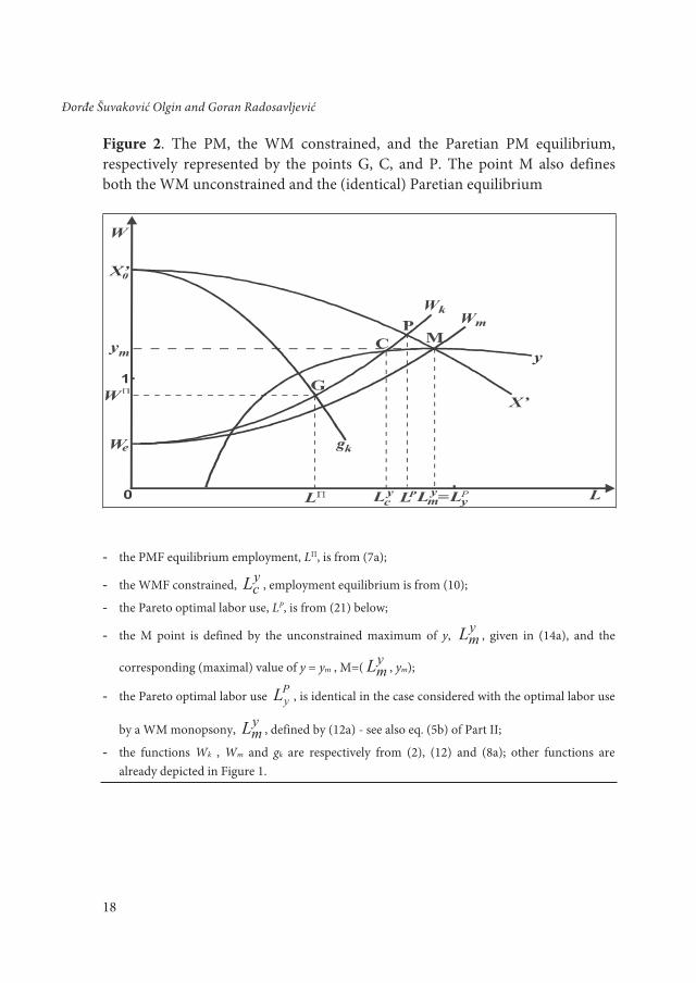
Figure 2. The PM, the WM constrained, and the Paretian PM equilibrium, respectively represented by the points G, C, and P. The point M also defines both the WM unconstrained and the (identical) Paretian equilibrium

- the PMF equilibrium employment, LП, is from (7a);

- the WMF constrained, ycL , employment equilibrium is from (10);

- the Pareto optimal labor use, LP, is from (21) below;

- the M point is defined by the unconstrained maximum of y, ymL , given in (14a), and the

corresponding (maximal) value of y = ym , M=( ymL , ym);

- the Pareto optimal labor use PyL , is identical in the case considered with the optimal labor use

by a WM monopsony, ymL , defined by (12a) - see also eq. (5b) of Part II;

- the functions Wk , Wm and gk are respectively from (2), (12) and (8a); other functions are already depicted in Figure 1.

1�


The required feature of the neutral Wn(L) function, where this feature is demonstrated in subsection 1.2 of Part IV4, is that it generates the maximum of

Π(L), ΠnL , equal to the unconstrained maximum of y, given in (12a):

( ) ( )[ ]ym

nn

LCLLWLXL

=

−−=Π maxarg (18)

Thus, an of (17) represents the degree of labor scarcity which yields the same equilibria for a PMF and WMF. The linear version of Wn(L) is depicted in Figure A1 of Appendix.

In what follows, we will denote by Sy the family that consists of disjoint

subfamilies cyS and u

yS , where, by analogy with the set notation5, we can write

uy

cyy SSS ∪= , OSS u

ycy /=∩ (19)

Given the definitions of cyS and u

yS of (13) and (16), the Sy subfamily may also

be written as:

Sy = {Wk = f(L, ak) ≡ Wk(L) , ak ∈ (an, az)} , (19a)

where az is that given by (5).

Finally, we introduce the remaining subfamily of S, denoted by SΠ, and making again the analogy with the set notation, we may write

SΠ = S \ Sy (20)

or, via the typical wage function Wk,

4 See equation (33) and the related part of the text. 5 Note however that one should always make a clear distinction between sets and families of

functions.


1�

SΠ = {Wk = f(L, ak) ≡ Wk(L) , ak ∈ (ae, an)}, (20a)

where ae and an respectively appear in (4) and (17).

4. The Alternating Dominance of a WM and PM Monopsony

4.1. The dominance of a WMF over PMF within the Sy subfamily of S

The dominance of a WMF over PMF within the cyS subfamily of S

In the model, for the typical wage function of S, the Pareto optimal employment, LP, depicted in Figure 2, is defined by the standard equation of Pareto optimum in the labor market:

LP = arg[X’(L) – Wk(L) = 0] , We ≤ Wk(L) ≤ Wz(L) (21)

At the same time, the local dominance of a WMF over PMF, or vice versa, is defined as follows:

Definition 1 - The Local Efficiency Dominance - Given the S family of wage functions, which all yield nonnegative profit both to a WMF and PMF, a WMF (PMF) is defined to locally efficiency dominate a PMF (WMF) if, for some function in S, a WMF (PMF) employs more labor, and thus produces more output and makes a greater total surplus than a PMF (WMF).

Now, starting from (1), we may write the first derivative of y(L) as:

( ) ( )L

LyLXLy −′≡′ )(

(22)

Also, solving (22) for X’(L) and substituting the latter into (8a), we can write the PMF equilibrium of (8a) in the form appropriate for a direct comparison of firms’ employment and output, and thus of efficiency:

Wk(L) = y(L) – L[W’k(L) – y’(L)] ≡ gk(L) , (23)

20


where in (23) the gk(L) function appears in a slightly different form than in (8a).

On the other hand, within the cyS subfamily of (13), the WMF constrained

equilibrium from (10) always satisfies the condition - see also point C in Figure 2:

Wk(L) = y(L) (24)

Now, within the relevant interval, given in (11), we have:

( ) ( ) ( )ymzk LLLLyLW ,,0 ∈>′>′ (25)

Hence, due to (25), it follows that in (23) the gk(L) function satisfies the following inequality:

gk(L) < y(L) , ( )ymz LLL ,∈ (26)

The monopsonistic PMF equilibrium, LП, obtained via the gk(L) function, is depicted in Figure 2 above, where the G point of this Figure may be written as G = (LП, WП), where:

LП = arg [gk(L) - Wk(L) = 0] , WП = Wk(LП) (27)

Now, since Wk is increasing in L, and due to (24), (25), (26) and (21), for any

wage function of cyS , a WMF has a higher employment, y

cL (and output) than

a PMF, LП, though less than the Pareto optimal one (LP):

LП < ycL < LP , (28)

where ycL is given in (10).

Finally, we summarize relation (28) by the following lemma:


21

Lemma 1. Within the cyS subfamily of wage functions a WMF efficiency

dominates a PMF.

The dominance of the WMF over PMF equilibrium within the cyS subfamily of

wage functions is depicted in Figure 2 above.

The dominance of a WMF over PMF within the uyS subfamily of S

Now we focus on the uyS subfamily of wage functions - defined in (16) - which

allow a WM monopsony to reach its unconstrained equilibrium but, as will be easily seen, still ensure the dominance of such a firm over its conventional PM twin.

A curious feature of the upper boundary function of uyS which, as already

pointed out, is Wm(L), is that it generates the identity of the Pareto optimal and WM equilibrium - due to (12a), (14) and (12) :

( ) ( ) ( ) ,LWLyLX ymm

ym

ymy ==′ (29)

where yX ′ denotes the WMF labor’s equilibrium marginal product.

At the same time, for the Wm(L) wage function, a PMF is still inferior to a WMF since, due to (8) and k = m, we have:

( ) ( ) ( ) ( ) ( )LXLWLWLLWLX ymmm ′=>′+=′Π , (30)

that is,

( ) ( ) ymmy LLLXLX <′>′ Π

Π = PL , (30a)

22


where Π′X denotes the PMF labor’s equilibrium marginal productivity and LP is the Pareto optimal labor use of (21).

Thus, it appears that there always exists some wage function - the Wm(L) function in our case - for which a non-wage-taking WMF reaches the Pareto optimum, and thus Pareto dominates the non-wage-taking PMF.

Furthermore, a decrease in the ak parameter from its am level does not affect the

WMF equilibrium, ym

y LL = .

On the other hand, a decrease in ak (expectedly) increases the PMF labor use, LП. To verify this, we write the PMF equilibrium of (8) as:

X’(L) = f(L, ak) + Lf’(L, ak) (31)

Then, we differentiate (31) with respect to ak and use the envelope theorem to obtain, due to (2c), (2a) and (9a):

02

<′′−′−′′

′+=

fLfXfLf

dadL kk aa

k (31a)

Thus, with ak decreasing from am of (12) to ae of (4a), the PMF equilibrium labor use, LП, is strictly monotonically increasing, until it (hypothetically) reaches its

wage-taking level ΠeL of (4a), where, due to X”< 0, we have:

yme LL >Π (32)

But, this further implies that there always exists some value an of the ak

parameter, where ae < an < am , and the corresponding neutral wage function Wn(L) ≡ f(L,an), already introduced in (17), which defines the identity between the PM and WM employment - see equation (18), which we write again here:

( ) ( )( ) ymnn LCLLWLXmaxargL =−−=Π (33)


23

In other words, within the Su family of wage functions there always exists a single wage function, Wn(L), which equalizes the PMF and WMF equilibrium and thus implies identical efficiency of the two types of firm. At the same time, note that Wn(L) divides the Sy

u family in the disjoint subfamilies Sy

u and SП, respectively defined in (16) and (20a).

We now collect the results of this subsection to obtain the following lemma:

Lemma 2. Within the Syu subfamily of wage functions a WMF efficiency

dominates PMF.

Finally, we integrate Lemma 1 and Lemma 2, to obtain:

Lemma 3. Within the Sy family of wage functions a WMF efficiency dominates

PMF, where, using again the set notation, uy

cyy SSS ∪= , OSS u

ycy /=∩ .

4.2. The dominance of a PMF over WMF within the SΠ subfamily of S and The Alternating Dominance Theorem

Due to the previous results, for the remaining SΠ subfamily of wage functions, defined in (20) and (20a), we immediately get the following lemma:

Lemma 4. Within the SΠ subfamily of wage functions a PMF efficiency dominates a WMF, where SΠ = S \ Sy, i.e., where Sy and SΠ are disjoint subfamilies.

Finally, we integrate Lemma 3 and Lemma 4 to get the general proposition on the alternating (efficiency) dominance of a WMF and PMF:

Proposition 1 - The Alternating Dominance Theorem. Given the income-per-worker function y = y(L), the continuous S family of all relevant wage functions - that make no losses both to a WMF and PMF - is divided by one, neutral member-function, Wn(L), into two disjoint subfamilies, Sy and SП , where for any function of Sy a WMF dominates PMF, while for any function of SП the converse is true.

24


In the next part we present systematic numerical simulations that provide an insight into the relative size of Sy and SП , and single out the major factors that explain this size.

5. The WMF/PMF Dominance Ratio, δ, and the size of the WMF and PMF Dominance Regions

We now temporarily assume that S is not a continuous but discrete family, characterized with a small uniform step in the ak scarcity parameter, ∆ ak = ∆ a, k = 1,…,n , where n is big. Thus we will have the (big number of) wage functions, evenly spread across S.

In principle, to measure the (approximate) size of relevant subfamilies one can count the wage curves that belong to these subfamilies6.

In order to calculate the WMF/PMF dominance relation, we first introduce what seems to be its natural definition:

Definition 2. The WMF/PMF dominance relation is identified with the δ ratio, where the numerator and denominator of δ respectively reduce to the shares of Sy and SП in S, and where these shares, denoted by N(Sy) and N(SП), represent the size of the WMF and PMF dominance regions,

)()(

Π=

SNSN yδ , (34)

where:

δδ+

=1

)( ySN , δ+

=Π 11)(SN (35)

6 Given the total of 30 simulations, see Tables 1-3 and Footnote 11 below, we had to omit the

counting procedure. Instead, as approximation, we have applied the Borell measure, which is error-free in the case of continuous families, while in the (present) discrete case it makes the computational error arbitrarily small, provided the number of family-member functions is arbitrarily big.


25

The δ dominance ratio also suggests introducing the concept of global efficiency dominance, as distinct from local dominance:

Definition 3. Given the S family of wage functions, a WMF (PMF) is defined to globally dominate PMF (WMF) if the δ dominance ratio is greater (smaller) than unity.

To get an idea about the magnitude of the δ ratio and about the major factors that explain this magnitude, we present in Tables 1-3, displayed at the end of this section, the corresponding systematically organized numerical simulations. A few of them are also graphically presented in Appendix.

First, the simulations examine the sensitivity of δ to switches from technologies T1, in which labor’s marginal productivity X’(L), is a strictly concave function of to T2 technologies, typical of linear X’(L), and, finally, to technologies with a strictly convex X’(L). Of course, the technologies are selected so as to be commensurable, in the sense that - given the price of output p(=1), fixed capital costs, C, and the entry-wage, We - they yield income per worker functions, characterized by (approximately) the same maximum, Ly

m( ≈ 1.98), and the same (maximal) value of income per worker, computed at this maximum, ym( ≈ 1.26).

The changes in δ due to switches of technologies can be seen by looking at any row of Tables 1-3.

Second, the simulations focus on the sensitivity of δ to changes in the degree of curvature of the family-member (inverse) labor supply or wage functions. These functions are first assumed to be linear, S1, then quadratic, S2, and, finally, cubic, S3. Here, the resultant changes in δ can be seen by looking at any column of Tables 1-3.

Third, simulations examine the sensitivity of δ to changes in the entry wage, We, that assumes values of 0.4 (Table 1), 0.63 (Table 2) and 1.0 (Table 3), which respectively comprise around 30%, 50% and 80% of the maximal income per worker, ym ≈ 1.26. Here, the underlying changes in δ can be seen by looking at its particular values in each field of Table 1, and then in the corresponding field in Tables 2 and 3.

26


What can first be concluded from the performed simulations is that the changes in δ assume the following regularities:

i) δ increases by switching from T1 to T2, and, then, from T2 to T3

technologies; ii) δ increases with the curvature of the wage functions, i.e., by switching from

linear to quadratic and, then, to cubic wage functions; iii) A fall in the entry wage, We leads to an increase in the δ ratio.

As for the direction and magnitude of the δ ratio, it appears that a WM monopsony strongly dominates its profit-maximizing twin7.

Thus, the WMF dominance region is (significantly) greater than that of a PMF in 26 of 27 simulations performed.

Finally, the average magnitude of the δ dominance ratio, denoted by δ and based on all 27 simulations, is very high and implies that, on average, around 94% of all the wage functions considered belong to the WMF dominance regions8.

In Appendix we graphically present the WMF and PMF dominance regions, obtained for We=0.4, linear X’(L) and, respectively, for the families of linear, quadratic and cubic wage functions.

7 The values of δ=δij (i,j=1,2,3), and thus of N (Sy), are approximate - see Footnotes 6 above

and 11 below. 8 To test the robustness of the performed simulations, we have also done the three modified

exercises, where the (previously parametric) entry-wage has been modeled as an increasing function of the labor scarcity parameter. The simulations have been designed to be comparable with the three arguably most representative simulations - of column 2, Table 2. However, this exercise has not altered the tenor of the previous results - the WMF average dominance region has become 91%, comparing to 93% of the corresponding fixed entry wage simulations.


2�

Table 1. The values of the δ dominance ratio for the entry-wage We = 0.4; δ = δij (i,j=1,2,3) is of Definition 2 of Part V. The technologies T1, T2 and T3, and the wage functions S1, S2 and S3, are also of Part V.

We = 0.4

T1 X’ = 3.5 – 0.6L2

y = 3.5 – 0.2L2 – C/LC = 2.85

T2 X’ = 2 – 0.4L y = 2 – 0.2L – C/LC = 0.680

T3 X’ = 2.08/(1.45L0.2) y = (2.6/1.45L0.2)–C/L C = 0.600

an = 0.231 az = 0.505

an = 0.160 az = 0.743

an = 0.227 az = 0.980

S1 Wn = We + an L Wz = We + az L δ11 = 1.19 δ12 = 3.64 δ13 = 3.32

an = 0.0803

az = 0.344 an = 0.0850 az = 1.01

an = 0.0790 az = 1.86

S2 Wn = We + an L2

Wz = We + az L2 δ21 = 3.28 δ22 = 10.9 δ23 = 22.5 an = 0.0314 az = 0.261

an = 0.0350 az = 1.61

an = 0.0314 az = 4.15

S3 Wn = We + an L3

Wz = We + az L3 δ31 = 7.31 δ32 = 45.0 δ33 = 131 Table 2. The values of the δ dominance ratio for the entry-wage We = 0.63; δ = δij (i,j=1,2,3) is of Definition 2 of Part V. The technologies T1, T2 and T3, and the wage functions S1, S2 and S3, are also of Part V.

We = 0.63

T1 X’ = 3.5 – 0.6L2

y = 3.5 – 0.2L2 – C/LC = 2.85

T2 X’ = 2 – 0.4L y = 2 – 0.2L – C/LC = 0.6800

T3 X’ = 2.08/(1.45L0.2) y = (2.6/1.45L0.2)–C/L C = 0.600

an = 0.171 az = 0.363

an = 0.172 az = 0.490

an = 0.166 az = 0.628


an = 0.0595 az = 0.231

an = 0.0620 az = 0.564

an = 0.0580 az = 1.00

S2 Wn = We + an L2

Wz = We + az L2 δ21 = 2.88 δ22 = 8.10 δ23 = 16.2 an = 0.0232 az = 0.161

an = 0.0250 az = 0.756

an = 0.0230 az = 1.86

S3 Wn = We + an L3

Wz = We + az L3 δ31 = 5.94 δ32 = 29.2 δ33 = 79.9

2�


Table 3. The values of the δ dominance ratio for the entry-wage We = 1; δ = δij (i,j=1,2,3) is of Definition 2 of Part V. The technologies T1, T2 and T3, and the wage functions S1, S2 and S3, are also of Part V.

We = 1

T1 X’ = 3.5 – 0.6L2

y = 3.5 – 0.2L2 – C/LC = 2.85

T2 X’ = 2 – 0.4L y = 2 – 0.2L – C/LC = 0.680

T3 X’ = 2.08/(1.45L0.2) y = (2.6/1.45L0.2)–C/L C = 0.600

an = 0.0750 az = 0.149

an = 0.0720 az = 0.168

an = 0.0690 az = 0.195


an = 0.0260 az = 0.085

an = 0.0260 az = 0.136

an = 0.0240 az = 0.204

S2 Wn = We + an L2

Wz = We + az L2 δ21 = 2.27 δ22 = 4.23 δ23 = 7.50 an = 0.0102 az = 0.0510

an = 0.0110 az = 0.124

an = 0.00900 az = 0.245

S3 Wn = We + an L3

Wz = We + az L3 δ31 = 4.00 δ32 = 10.3 δ33 = 26.2

6. Summary and Concluding Remarks

In this paper we have compared the short-run efficiency of profit- and wage-maximizing firms (PMFs and WMFs) when they operate at the monopsonistic labor market. To perform the comparison, we have first ruled out any type of wage discrimination as well as the (possible) existence of a market for WMF membership rights. We have then defined local efficiency dominance, according to which one no loss making firm dominates the other when, for a single inverse labor supply or wage function, the former produces more output - and thus creates a greater total surplus - than the latter.

For well-behaved wage functions we have then varied a suitably defined labor scarcity parameter, from zero to its zero-profit level. Given a turned U-shaped income-per-worker schedule, the latter level defines the steepest wage curve that yields zero profit both to a WMF and PMF, and therefore has a tangency point with the income-per-worker schedule. We have thus generated the continuous family of wage functions, all of which ensure nonnegative profit for a PMF and WMF where, by definition, the number of such functions is infinite.


2�

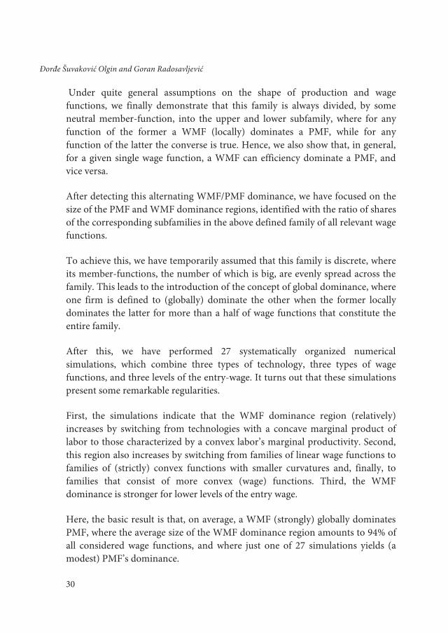
Under quite general assumptions on the shape of production and wage functions, we finally demonstrate that this family is always divided, by some neutral member-function, into the upper and lower subfamily, where for any function of the former a WMF (locally) dominates a PMF, while for any function of the latter the converse is true. Hence, we also show that, in general, for a given single wage function, a WMF can efficiency dominate a PMF, and vice versa.

After detecting this alternating WMF/PMF dominance, we have focused on the size of the PMF and WMF dominance regions, identified with the ratio of shares of the corresponding subfamilies in the above defined family of all relevant wage functions.

To achieve this, we have temporarily assumed that this family is discrete, where its member-functions, the number of which is big, are evenly spread across the family. This leads to the introduction of the concept of global dominance, where one firm is defined to (globally) dominate the other when the former locally dominates the latter for more than a half of wage functions that constitute the entire family.

After this, we have performed 27 systematically organized numerical simulations, which combine three types of technology, three types of wage functions, and three levels of the entry-wage. It turns out that these simulations present some remarkable regularities.

First, the simulations indicate that the WMF dominance region (relatively) increases by switching from technologies with a concave marginal product of labor to those characterized by a convex labor’s marginal productivity. Second, this region also increases by switching from families of linear wage functions to families of (strictly) convex functions with smaller curvatures and, finally, to families that consist of more convex (wage) functions. Third, the WMF dominance is stronger for lower levels of the entry wage.

Here, the basic result is that, on average, a WMF (strongly) globally dominates PMF, where the average size of the WMF dominance region amounts to 94% of all considered wage functions, and where just one of 27 simulations yields (a modest) PMF’s dominance.

30


Thus - in the broader context, and on the theoretical level - we have shown that for monopsonized labor market there exists a type of maximizing behavior (often discussed in the corresponding literature), where this behavior may well be superior to conventional profit-maximization.

Finally, two notes on the novel concept of global efficiency dominance are in order.

First, the concept does not seem to be restricted to the present case of monopsonistic labor markets and could also be used under some other market structures, e.g. under monopoly and monopolistic competition.

Second, on the empirical level, the concept would require each family-member function to be weighted by the probability of its occurrence at the market in question. Still, on the theoretical level, here considered, the (implicitly) assumed equal probability of all member-functions seems legitimate. This is due to the fact that all considered wage functions enable firms to make no losses, and from this perspective it seems reasonable not to discriminate between them, at least not on this stage of analysis.

The third note may be of relevance for the theory and policy of privatizing a non wage-taking firm, which is supposed to be the wage maximizer. If in such a case one reveals the local dominance of a WMF over PMF, a higher local efficiency of the former - due to its objective of wage maximization - ought to be weighed against the possibly higher technical productivity of the latter, observed in many outsider-privatized PM firms (see, for example, Frydman, Gray, Hessel and Rapaczynski (1999)).

In any case, and irrespective of these remarks, the key result of the paper clearly points to the fact that in non-wage-taking environments, and with equal technical and market opportunities, a wage-maximizing firm may be more efficient, both locally and globally, than a conventional, profit-maximizing enterprise.


31

32


Bhaskar, V., Manning, A. and To T. (2004), 'Oligopsony and the Monopsonistic Competition in Labor Markets', mimeo.

Blanchard, O. (1��), The Economics of Post-Communist Transition, Clarendon Press

Boal, W. and Ransom, M. (1��), “Monopsony in the Labor Market”, Journal of Economic Litera-ture, 35, �6-112.

Boal, W. and Ransom, M. (2002), “Monopsony in American Labor Markets”, EH.NET’s Online Encyclopedia of Economic History

Bonin, J. and Putterman, V. (1��), Economics of Cooperation and the Labor-Managed Economy, Harwood Academic Publishers

Bonin, J., Jones, D. and Putterman, L. (1��3), ’Theoretical and Empirical Studies of Producer Co-operatives: Will Ever the Twain Meet?’ Journal of Economic Literature, 33, 12�0-320.

Domar, E. (1�66), “The Soviet Collective Farm as a Producer Cooperative”, American Economic Review, 56, �34-5�.

Dreze, J. (1��), Labor-Management, Contracts and Capital Markets: A General Equilibrium Ap-proach, Basil Blackwell

Frydman, R., Gray, C., Hessel, M. and Rapaczynski, A. (1��), “When does Privatization Work? The Impact of Private Ownership on Corporate Performance in the Transition Economies”, Quar-terly Journal of Economics, 114, 1153-�2.

IBRD (1��6), World Development Report 1996: From Plan to Market, Oxford University Press

Manning, A. (2003a), Monopsony in Motion: Imperfect Competition in Labor Markets, Princeton University Press.

Manning, A. (2003b), “The Real Thin Theory: Monopsony in the Modern Labour Markets”, La-bour Economics, 10, 105-131.

Pencavel, J. and Craig, B. (1��4), “The Empirical Performance of Orthodox Models of the Firm: Conventional Firms and Worker Cooperatives”, Journal of Political Economy, 102, �1�-44.

Roland, G. (2000), Transition and Economics: Politics, Markets and Firms, MIT Press

Staiger, D., Spetz, J. and Phibbs, C. (1��), ’Is There Monopsony in the Labor Market? Evidence from a Natural Experiment’, NBER Working Paper �25�.

rEfErEnCES

APPENDIX: A graphical presentation of the WM and PM dominance regions for the three types of wage functions9

Figure A1. The WMF and PMF dominance regions, identified with the Sy and SП subfamilies of the discrete S family, are approximated by the darker and lighter shaded areas, bordered by the Wz, Wn, and We functions: The case of linear labor’s marginal product and linear wage functions, δ12 = 3.64, see Table 1 of Part V.

X = 2L – 0.2L2 - production function X’ = 2 – 0.4L - labor’s marginal product y = 2 – 0.2L – C/L - income per worker C = 0.68 - fixed costs We = 0.4 - entry wage horizontal line, ak = 0 ak = a - typical (varying) labor scarcity parameter Wk = We + akL2 - typical wage function Wn = We + anL - neutral wage function that implies equal equilibrium of WMF and PMF, an = 0.160

9 Note that in this Appendix the product price is p=1. Also, as mentioned in Part V, the

maximum point of income per worker is approximately the same in all Figures: M = (Lmy, ym) ≈ (1.98, 1.26).

30

1

X’

yWn

We

Wz

Z

W

LL LeLz

E

Mym

my


33

Wz = We + azL - wage function that implies zero-profit and identical equilibrium of a WMF and PMF, az = 0.743

Figure A2. The WMF and PMF dominance regions, identified with the Sy and SП subfamilies of the discrete S family, are approximated by the darker and lighter shaded areas, bordered by the Wz, Wn, and We functions: The case of linear labor’s marginal product and quadratic wage functions, δ22= 10.9, see Table 1 of Part V.

X, X’, y , C, We, ak, and Wk - as in legend of Figure A1 Wn = We + anL2 - neutral wage function, defined as in Figure A1, an = 0.085 Wz = We + azL2 - zero-profit wage function, defined as in Figure A1, az =1.01

34


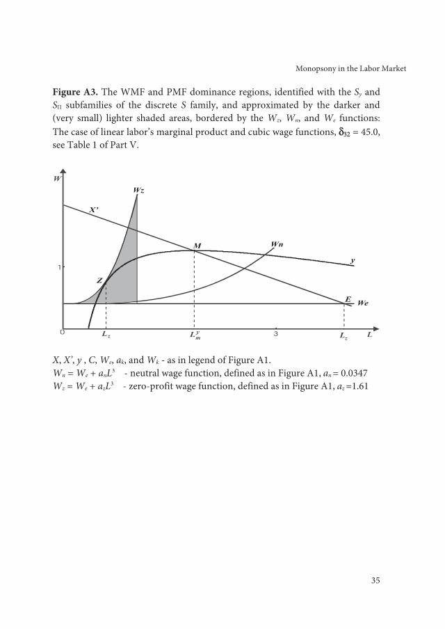
Figure A3. The WMF and PMF dominance regions, identified with the Sy and SП subfamilies of the discrete S family, and approximated by the darker and (very small) lighter shaded areas, bordered by the Wz, Wn, and We functions: The case of linear labor’s marginal product and cubic wage functions, δ32 = 45.0, see Table 1 of Part V.

X, X’, y , C, We, ak, and Wk - as in legend of Figure A1. Wn = We + anL3 - neutral wage function, defined as in Figure A1, an = 0.0347 Wz = We + azL3 - zero-profit wage function, defined as in Figure A1, az =1.61

0 3

1


35

Date post:	27-Feb-2020
Category:	Documents
Upload:	others
View:	8 times
Download:	0 times

› img › doi › 0013-3264 › 2007 › 0013-32640773007S.pdf MOnOpSOny In thE LAbOr MArKEt:...

Documents