“A” is the Aim? - GWDG

ISSN: 1439-2305

Number 291 – October 2016

“A” IS THE AIM?

Kamila Danilowicz-Gösele

“A” is the Aim?

Kamila Danilowicz-Gosele1

October 2016

Abstract

This paper analyzes professors’ effect from a fundamental first-year course in Eco-

nomics on students’ later performance in follow-on courses with a special attention

given to the problem of self-selection bias of students toward certain professors.

Based on an extensive dataset consisting of administrative data on more than

2, 900 students from the university of Gottingen, an instrumental variable (IV)

strategy is used. The obtained results indicate that professors have powerful ef-

fects on students’ achievement. However, the sign of this effect is ambiguous, and

depends on the mathematical rigor of the course and the examination style.

Keywords: university, education, grade inflation

JEL classification: I23, I21, I28

1Chair of Public Economics, Georg-August University Gottingen, [email protected]

1

1 Introduction

Academic grades are said to reflect students’ achievement and thereby the effectiveness

of educational institutions and their accountability to potential employers. However, in

the past decades, confidence in the reliability of the grades has been badly shaken by

studies exposing the trend towards grade inflation. Several studies have shown that rise

in grades has become an issue in both secondary and tertiary education across many

countries, thereby stressing the need to provide explanations for the phenomenon of

grade inflation. Rojstaczer and Healy (2010) conducted a study of grading patterns

in more than 160 American colleges and universities and found a nationwide rise in

average grades of nearly a tenth of a point change per decade, with A being the most

commonly awarded grade at American colleges and universities.

This paper addresses this concern by focusing on the differences in grading poli-

cies between professors assigned to the same mandatory first-year course in Economics.

Firstly, the analysis reveals that there are huge differences in grading even within the

same course. Secondly, the effect of having a certain professor in the mandatory first-

year course on student’s later performance is highly significant and cannot be solely

explained by differences in professors’ grading. However, the sign of this effect is am-

biguous, and depends on the mathematical rigor of the course and the examination

style. Furthermore, the results demonstrate a highly significant effect of having the

same professor for many classes, although switching from a tough to an easy grader

seems to be the best strategy for improving grades. Our analysis shows that the ob-

tained effects are quite meaningful. All else being equal, having a certain professor in

Microeconomics I is associated with an improvement of the expected grade in a follow-

on course by up to 1.385 grades. The overall result indicates that both grading policies

and learning outcomes vary between professors within the same course.

When talking about grade inflation, it is important to distinguish between awarding

higher grades per se and improvement in grades as a result of better performing stu-

dents who are learning more and/or being taught better. The difficulty with the latter

explanation lies in the fact that a growing number of educational researchers claim

that it is raining A’s in the education system without continuous evidence of increasing

academic performance.

Strong evidence that students are indeed doing worse today relative to a decade

ago is provided by researchers from the National Center for Education and Statistics

in 2015, who claim that SAT scores in critical reading, writing and math have dropped

2

each year within the analyzed period from 2004 till 2012 (Kena et al., 2015). Moreover,

according to the report published by the National Bureau of Economic Research of the

University of California, students decreased their class and studying time from 40 hours

per week in 1961 to 27 hours per week in 2003 (Babcock and Marks, 2011).

Since concerns about grade inflation are not new, researchers have already offered

many explanations for the upward trend in grades. Some of these explanations focus on

changes in educational institutions including changes in enrollment patterns (Prather

and Kodras (1979)), curricula (Prather and Kodras (1979)) or grading policies (Birn-

baum (1977)).

Although the teaching body is expected to individually regulate grading policies,

because of their effect on the reputation of the institutions they work for and students’

career chances, it is commonly known that unregulated institutions are very often chal-

lenged to maintain certain continuous standards. This is also the case for the colleges

and universities, which have troubles maintaining academic standards in the absence

of any regulation. Against this background, educational researchers found out that

teachers’ characteristics such as teaching quality (De Paola (2009)), teaching experi-

ence (Rivkin et al. (2005); Clotfelter et al. (2007)), gender (Neumark and Gardecki

(1998); Bettinger and Long (2005); Carrell et al. (2010)) and age (?), have statistically

significant effects on students’ grades. However, there is less agreement on the influence

of the instructor rank (Sonner (2000)), part-time or full-time status or salary (Nelson

and Lynch (1984); Pressman (2007); Hoffmann and Oreopoulos (2009)). In addition,

there is strong evidence that changes in the use of student evaluations (Krautmann and

Sander (1999); Stratton et al. (1994); Johnson (2003) and Eiszler (2002)) or the public

availability of median grades (Bar et al. (2009)) may also influence the extent to which

instructors exaggerate students’ grades.

Other kinds of explanations draw attention to changes in students’ behavior includ-

ing students’ freedom in choosing departments, courses or certain professors. At many

universities, there is a visible trend towards learning that is more relevant to students’

interests and goals. Therefore, today’s students have much more freedom in designing

their study paths, being able to choose from a wide range of major/elective courses de-

pendent on their interest, abilities, difficulty level, instructor, work load or examination

structure. In some cases, they can even decide whether the grade from a taken class will

appear on their transcript of records or not. Thus, in order to improve the overall grade,

students may act strategically by taking advantage of the mentioned differences, which

will result in attending carefully-selected courses or in opting for non-visible grades.

3

The study of Sabot and Wakeman-Linn (1991) shows that students are significantly

more likely to enroll in a subsequent course of a department where they have already

received a relatively higher grade. Another finding of their study is that grades obtained

in low-grading departments are better predictors of students’ later performance than

grades received from grade-deflating departments. A similar finding is reported in a

study of Ost (2010), who found out that low grades in science classes can be used as a

predictor for students’ participation in subsequent science courses.

Given all this, it is not surprising that, in many countries, such as United States,

Canada, England, Scotland and Wales, online professor rating sites, such as “Rate

My Professors.com”, become so popular. In this case, students have the possibility to

rate their professors according to easiness, helpfulness, clarity, hotness and the rater’s

interest in the class, in order to help fellows to choose the appropriate classes and/or

professors. Some studies, such as Miles and Sparks (2013), examined the effect of

online professor ratings and found out, that such websites indeed have an influence on

students’ choices for selecting professors, however it is not very clear to what extent.

Although there is a vast amount of research on grade inflation, there is little at-

tention to grading differences within higher education, especially within the same field

of study or within the same course. This paper contributes to this body of literature

by assessing the effect of grading and teaching differences from a mandatory first-year

course on students’ performance in follow-on courses at a German University. Even

though all professors assigned to the mandatory first-year course have a very similar

teaching and examination style, and students in most cases follow the curriculum, there

is no random placement of students into the classroom and thus have to be aware of

students’ self-selection toward certain professors. For this reason, this paper proposes

a instrumental variable (IV) strategy by instrumenting student’s choice of a professor

through a random assignment of professors, on the semester basis, to the mandatory

first-year course. In this case, we follow the faculty’s recommendation to write the exam

in the second semester of studies. Therefore, taking the exam with a professor who was

assigned to the course in the student’s second semester will influence the student’s later

performance. On the contrary, the fact that a professor is assigned to the course in the

student’s second semester does not affect the student’s later achievements if a student

decides, against the faculty’s recommendation, to write her exam in an earlier or later

semester.

The paper is organized as follows: Section 2 provides a brief overview of the in-

stitutional background. The data set, variables used and the empirical framework are

4

presented in Section 3. Section 4 presents the results and Section 5 concludes with

summarizing the findings of the analysis.

2 Institutional Background

Since the aim of the paper is to study the differences in professors’ grading and its effect

on students’ performance in follow-on classes, this paper chooses one of the mandatory

first-year courses offered at the faculty of Economics, namely Microeconomics I. It

is an introductory undergraduate course that teaches the fundamentals of microeco-

nomics. The reasons for our choice are three-fold. Firstly, this course is mandatory

for all students enrolled at the faculty of economic sciences at Gottingen University,

thus providing us with extensive and diverse observations. Secondly, within the fac-

ulty of economic sciences, Microeconomics I is the course with the greatest number of

professors assigned, thus indicating variation according to their characteristics such as

grading policy. Last but not least, since Microeconomics I is one of the first courses

economic students are required to take in their undergraduate programs, it also serves

as a prerequisite for many follow-on classes. Therefore, its accompanying effect of dif-

ferent grading policies, if existent, should be strong enough to be observed in students’

later achievements.

Based on the explicit information provided on students’ university records, we are

able to restrict our analysis to students enrolled at the faculty of economic sciences

who have participated in the Microeconomics I exam either once or multiple times but

always with the same professor.

Although professors’ assignment to the Microeconomics I course is to a greater

extent random and thus not known in advance to the students, we are still aware of the

self-selection bias toward certain professors. The reason for this is that, students are,

to some extent, free to choose when they want to take this course. The only restricting

factor is the examination regulation, according to which the credits for this course must

be earned by the end of the student’s fifth semester. For this reason, they can postpone

taking the course to a later semester or even after taking the class in their second

semester they can still decide to drop-out of the exam. In fact, it might be tempting

for some students to postpone the Microeconomics I exam until a professor, known for

“easy grading”, will offer it.

In order to control for students’ potential self-selection bias, we follow the recom-

5

mendation of the Economics faculty. Hence, in our analysis we will distinguish between

students who followed faculty’s recommendation and students who postponed the exam

to a later date. In addition to this we could also think about other factors, such as

illness or other circumstances beyond students’ control, that lead to postponing the

exam.

The follow-on courses that we decided to look at are Microeconomics II and Public

Finance, the latter one combines the introductory and the advanced course which are

both taught by the same professor. Both courses aim to further deepen the study in

microeconomics, thus having Microeconomics I as a prerequisite. All examined courses

have a similar structure and consist of lecture and tutorials on a weekly basis. The

lectures are taught by one of the university professors, tutorials, however, are taught

either by scientific assistants (Public Finance) or trained students who already passed

the respective course (Microeconomics I and II).

3 Data and Methodology

3.1 Dataset and descriptives

Dataset

This paper employs a unique administrative data set of 2, 920 students enrolled at

the faculty of economic sciences of the Gottingen University who participated in the

Microeconomics I exam between 2006 and 2011.1 The detailed and anonymized data

includes students’ characteristics such as high school leaving degree, gender, type of

health insurance or parental address, as well as students’ university records such as

chosen field of study, grades, examiners, attempts and examination dates.

Dependent Variables

Our outcome variables are students’ grades from three undergraduate courses offered

at the faculty of economic sciences, namely Microeconomics I, Microeconomics II and

Public Finance.

The data set is restricted to students who either took the exam in Microeconomics

I one time or multiple times but always with the same professor. In case of multiple

1Gottingen is a small city in Lower Saxony (Germany) where students account for 22% of thecity’s population (Statistisches Bundesamt, 2009). According to the statistics of the University ofGottingen, there are currently more than 4,300 students enrolled at the Faculty of Economic Sciences,which amounts to around 15 percents of all students on campus.

6

examination attempts, we will use the grade a student received on her first examination

attempt in this course, implying that every student in our data has only one grade in

Microeconomics I.

For the two other courses, Microeconomics II and Public Finance, we will use the

best grade the student received in all her attempts.

In order to make the results internationally comparable, German grading scale,

with 1.0 as the best possible grade and 4.0 as the minimum passing grade, has been

translated to the U.S. grading scheme.

Independent Variables

Within the analyzed period from 2006 to 2011, five different professors were assigned

to teach the Microeconomics I course. To include these in our analysis, we create

an indicator variable for each professor, reflecting the student’s enrollment decision

concerning Microeconomics I. For example, if a student took her first Microeconomics

I exam with Professor 1, her indicator variable for this professor will equal one. Con-

sequently, the remaining four indicator variables (Professor 2; Professor 3; Professor

4; Professor 5) will be zero.

Assuming that students can benefit from having the same professor in different

subjects, we include one further indicator variable Same Professor to capture the effect

of having the same professor in the two analyzed courses.

The high school grade point average (GPA) will be used as a control for students’

ability. GPA serves as a predictor of academic success believing that this measure cap-

tures more than just the students’ abilities or achievements but also certain behavioral

factors. Likewise course grades, high school GPA is converted to the U.S. grading scale.

In the analysis, we also account for students’ socio-economic background by using

the students’ health insurance type and the purchasing power index of her parents’ zip-

code area. The type of health insurance is suited as a proxy for students’ educational

and socio-economic background because of the organization of the German health care

insurance system, which is characterized by the dual system of public and private health

insurance. While almost everyone is eligible for public health insurance, the private

health insurance can be chosen only due to certain income criteria or employment

status.2. Since in most cases students are insured through their parents, their health

2In 2008 the number of people being privately insured (civil servants, self-employed or high earners)with a university degree was almost three times as high as that within the total German population(Finkenstadt and Keßler (2012); Statistisches Bundesamt (2009))

7

insurance status also provides information about their educational background.

Additionally, the purchasing power index within the zip-code area of the students’

home address serves as another compelling measure of students’ socio-economic back-

ground, considering that the German zip-code areas are fairly small and assuming that

there is some residential sorting due to income. It relates to the per-capita income of a

zip-code area with the average per-capita income of Germany, thus expressing the pur-

chasing power of a region. The index is normalized to 100, meaning that an area with

an index value of 110 has a purchasing power of greater than ten percent as compared

to the German average.

Furthermore, since there is a lack of agreement in educational research about

gender differences we include gender as a control variable in our analysis. Gender is

measured as a dichotomous variable coded as 1 for female and 0 for male.

Summary Statistics

The summary statistics in Table 1 show that the number of observations in the two

analyzed follow-on courses, Microeconomics II and Public Finance, does not equal our

sample size in Microeconomics I. This is due to the fact that study and examination

regulations vary among degree programs at the faculty of economic sciences, meaning

that some courses are not necessarily required as part of undergraduate studies.

For Microeconomics I, the mean-value for a sample of 2, 920 students is 2.12. For

Microeconomics II, the mean-value for a sample of 1, 255 students is 2.03 and thus

only slightly lower than the mean-value of Microeconomics I. The highest mean-value

of 2.33 appeared for a sample of 964 students in Public Finance.

Nearly half of the students in the sample took their Microeconomics I exam with

Professor 1, and one third of the students with Professor 5. Possible explanations for

these differences in the attendance rates include the fact, that these both professors

offered this course more often.

In our sample the mean-value of High School GPA is approximately 2.5 which is

higher, meaning better, than the mean of the grades obtained in Microeconomics I,

Microeconomics II and Public Finance, respectively. This can be explained by the fact

that a grade of 0.0, meaning failed, is not possible for the high school leaving certificate.

The share of female students in all courses is about 40 percent. The purchasing power

index is slightly lower for students in the Public Finance class and almost the same

for students in Microeconomics I and in Microeconomics II. Microeconomics I has the

lowest share of students with a private health insurance.

8

Table 1: Summary Statistics

Variable Observations Mean Std. Dev. Min Max

Grade in Microeconomics I 2920.00 2.12 1.11 0.00 4.00

High School GPA 2920.00 2.46 0.55 1.20 4.00

Female 2920.00 0.41 0.49 0.00 1.00

Private Health Insurance 2920.00 0.17 0.38 0.00 1.00

Purchasing Power Index 2920.00 99.09 11.76 70.16 258.82

Prof. 1 Dummy 2920.00 0.43 0.49 0.00 1.00

Prof. 2 Dummy 2920.00 0.10 0.30 0.00 1.00

Prof. 3 Dummy 2920.00 0.07 0.25 0.00 1.00

Prof. 4 Dummy 2920.00 0.11 0.31 0.00 1.00

Prof. 5 Dummy 2920.00 0.30 0.46 0.00 1.00

Easy Graders Dummy 2920.00 0.41 0.49 0.00 1.00

Tough Graders Dummy 2920.00 0.59 0.49 0.00 1.00

Grade in Microeconomics II 1255.00 2.03 1.13 0.00 4.00

High School GPA 1255.00 2.46 0.58 1.20 4.00

Female 1255.00 0.39 0.49 0.00 1.00



Prof. 1 Dummy 1255.00 0.38 0.48 0.00 1.00

Prof. 2 Dummy 1255.00 0.06 0.25 0.00 1.00

Prof. 3 Dummy 1255.00 0.03 0.16 0.00 1.00

Prof. 4 Dummy 1255.00 0.18 0.39 0.00 1.00

Prof. 5 Dummy 1255.00 0.35 0.48 0.00 1.00



Grade in Public Finance 964.00 2.23 1.07 0.00 4.00

High School GPA 964.00 2.50 0.57 1.20 4.00

Female 964.00 0.40 0.49 0.00 1.00



Prof. 1 Dummy 964.00 0.37 0.48 0.00 1.00

Prof. 2 Dummy 964.00 0.05 0.22 0.00 1.00

Prof. 3 Dummy 964.00 0.03 0.17 0.00 1.00

Prof. 4 Dummy 964.00 0.19 0.39 0.00 1.00

Prof. 5 Dummy 964.00 0.35 0.48 0.00 1.00



Grades transformed to 1-4 Scale, with 4 being the best grade and 1 being the worst grade

that is still considered a pass. A grade of 0 means that the student failed the respective

course.

3.2 Empirical Approach

In fact, we do not have course placement in the sense of a random assignment, meaning

that the students could up to some extent freely decide on the timing of their exams

and hence choose professors they want to write the exams with. Thus, although we

cannot observe any assignment pattern, students’ long-term expectations about who

will teach Microeconomics I in following semesters should not be underestimated. In

order to control for the potential self-selection bias of the students, we will follow the

faculty’s recommendation to take the Microeconomics I exam in the second semester

of undergraduate studies.

9

In our analysis, we first examine the grading policy of the five professors assigned

to Microeconomics I. Since we first want to analyze how does tough or easy grading

from a fundamental undergraduate course correspond to students’ later university per-

formance, we divide the sample of professors in two groups (Tough Graders vs. Easy

Graders) according to their grading standards. To examine the effect of having a

Tough Grader/Easy Grader in Microeconomics I on the grade obtained in the respec-

tive follow-on class, ordinary least square (OLS) regressions are applied. Thus, in the

baseline empirical model, student’s performance can be described using a linear rela-

tionship with student’s grade from a single class as the dependent variable and a vector

of independent variables. The baseline model is then given by

yic = β0 + β1GPAi + β2Si + β3Pi + εi (1)

where yic is the grade for student i in course c; GPAi is the GPA of student i; Si is a

vector of individual characteristics of i such as gender and socio-economic background,

Pi is the dummy variable either for the professor the student i wrote her Microeco-

nomics I exam with or for the group (Tough Graders/Easy Graders) her professor

belongs to; εi is an error term. In all regressions, robust standard errors are clustered

by semester. However, since the number of clusters is less than 30, it is possible that the

estimated standard errors are biased downward. Therefore, we follow (Cameron et al.,

2008) and report the wild bootstrap p-values below the coefficient estimates in brackets.

Instrumental Variables Regression (IV)

Estimates of β3, the coefficient of professor’s dummy variable from Microeconomics I

exam, may be biased under OLS regressions due to the potential self-selection bias of

students toward certain professors. For instance, if all weak students chose to write the

Microeconomics I exam with an Easy Grader, the professor’s effect in Microeconomics

II would be much more negative. For this reason we treat the professor’s dummy Pi

as an endogenous regressor, assuming that Pi and εi are somehow correlated. Since

we are treating Pi as endogenous, we need one or more additional variables that are

correlated with Pi but not correlated with εi. When analyzing grades obtained in the

Microeconomics II and the Public Finance exam, we group up professors according to

their grading standards, so that Pi from the baseline model will be then replaced by

P (tough)i representing the Tough Graders.

10

To account for the potential self-selection bias, we propose standard IV approach.

Implementing the IV approach requires a two stage least squares estimation (2SLS) to

be performed. This approach starts with the first stage of analysis, which is necessary

given that the potential self-selection of students toward certain professors may affect

both independent and dependent variables. In the first stage P (tough)i becomes the

dependent variable and the independent variables include all control variables from

the second stage as well as the instrumental variable. Addressing the faculty’s rec-

ommendation to write the Microeconomics I exam in the second semester, we create

an instrumental variable, that is equal to one if a student took the Microeconomics I

exam with a professor who was supposed to offer this course in her second semester of

studies, and equal to zero otherwise. Therefore, taking the exam with a professor who

was assigned to the course in the student’s second semester will influence the student’s

later performance. On the contrary, the fact that a professor is assigned to the course

in the student’s second semester does not affect the student’s later achievements if a

student decides, against the faculty’s recommendation, to write her exam in an ear-

lier or later semester. The instrument should not have any influence on the outcome

variable. Moreover, these excluded exogenous variables must not influence grade yic

directly, otherwise they should be included in the Equation 1. Since we have five dif-

ferent professors assigned to the Microeconomics I exam, we will have five instrumental

variables, one for each professor. Therefore, the endogenous regressor Tough Graders

will be instrumented by three (Professor 1; Professor 2 and Professor 3) additional

exogenous variables.

The first stage equation looks as follows:

P (tough)i = πo+π1GPAi+π2Si+π3Professor1i+π2Professor2i+π3Professor3i+εi

(2)

The second stage implements the Equation 1, in which the dependent variable is

regressed on the predicted values from the first stage regression plus the control vari-

ables. It is assumed that the instrumental variables are uncorrelated with any omitted

variables, thus removing the bias in the relationship between student’s grade in a course

and student’s choice of the professor to write the exam with. In the following we will

apply the above instrumental approach to the subsamples of students who obtained,

besides the grade from the Microeconomics I, at least one grade in the Microeconomics

II and/or in the Public Finance exam.

An important condition to obtain consistent estimation is that the instruments are

11

not weak. This can be tested with the Kleibergen-Paap Wald rk F statistic, which

is a robust analog to the Cragg Donald statistic and thus superior in the presence

of heteroskedasticity, autocorrelation or clustering (Baum et al. (2007)). It is an F

statistic for the joint significance of the instruments in the first stage regression, which

tests whether the instruments jointly explain a sufficient amount of the variation in the

endogenous regressor. If the instruments are weak the standard errors can become

considerably larger and the t statistics considerably smaller than those from OLS,

indicating the loss of precision.

The other general specification is the Hansen test that implements a test of overi-

dentifying restrictions and is robust to heteroskedasticity. The null hypothesis of this

test is that instruments (overidentifying restrictions) are valid (Cameron and Trivedi

(2010)). Therefore the rejection of the null hypothesis is an indication that at least one

of the instruments is not valid.

4 Results

Having a certain professor in Microeconomics I exam may be associated with a differ-

ent grading and teaching style, which in turn will influence students’ performance in

follow-on courses. On the one hand, it is likely that students who took their Microe-

conomics I exam with a Tough Grader, and thus learned more, will perform better in

Microeconomics II exam. This would suggest that besides different grading policies, we

also find significant differences in learning outcomes. On the other hand, it may also

be that the students learned the same as they would with an Easy Grader and just got

a worse grade, which would simply refer to differences in grading policies.

4.1 Microeconomics I

By looking at students’ performance in Microeconomics I, we estimate the effect of

having a certain professor on the grade obtained from the first attempt in the Microe-

conomics I exam. This effect may arise from a number of professors’ characteristics,

for instance grading policy, teaching or examination style, or combination of those. For

this course, our benchmark student is male, holds a public private insurance and is

average with regard to all continuous variables.

The OLS estimation results can be found in Table 2. According to the results, the

choice of a professor in Microeconomics I has a significant impact on the grade achieved

12

in this subject. Hence, taking Microeconomics I exam with Professor 1, Professor 2 or

Professor 3 results in lower grades than writing the exam with Professor 5 (baseline).

Thus, professors seem to vary considerably in their grading standards, even within

a single course. This finding raises further questions whether the observed grading

differences have a significant influence on students’ later achievements.

Estimating the effect of professors’ grading standards on students’ later achieve-

ments assumes that these standards are relatively consistent over time, that they are

not affected by the composition of students attending the course. To analyze this, we

divided the sample of professors into two groups according to their grading standards

each semester and analyzed if their position changes over time. The first group, Tough

Graders, consists of Professor 1, Professor 2 and Professor 3, and the second group,

Easy Graders, of Professor 4 and Professor 5. We found that there was no movement

between those groups, which led us, since we are not primarily interested in professors’

individual characteristics, to use this classification for our subsequent analysis. It is

not surprising that, when including these two groups as control variables, one finds a

highly significant and negative effect of the Tough Graders on students’ obtained grade

in Microeconomics I.

In addition, we find the expected highly significant and positive effect of the high

school leaving grade as shown in Table 2. The higher the high school leaving grade, the

better the grade the student obtains in Microeconomics I exam. Although the size of the

coefficient may appear to be somewhat large, it provides an indication that this course

is based on skills and methods already used in high school. For instance, Mathematics

serves as a prerequisite for all analyzed courses and is generally counted more heavily

in the calculation of the GPA. This result is consistent with the findings of a large body

of existing research (see, e.g., Cyrenne and Chan, 2012; Girves and Wemmerus, 1988).

Other controls are of lesser importance. The gender as well as the socio-economic

variables, private health insurance and the purchasing power index of parents’ zip-code

area, do not show a significant effect in any of the regressions based on conventional

hypothesis tests that are presented in Table 2. However, the purchasing power index

is significant at the 5 percent level based on wild bootstrap p-values. These overall

findings are in line with Danilowicz-Gosele et al. (2014) who found that socio-economic

factors are, if at all, poor indicators of students’ university performance.

13

Table 2: OLS regression estimates for Microeconomics I

Dependent variable: Grade in Microeconomics I(1) (2) (3) (4)

High School GPA 0.716*** 0.713***(0.056) (0.055)[0.000] [0.000]

Female -0.0731 -0.0707(0.060) (0.061)[0.360] [0.360]

Private Health Insurance 0.0631 0.0604(0.038) (0.037)[0.160] [0.160]

Purchasing Power Index 0.00243 0.00258(0.001) (0.001)[0.040] [0.040]

Course Assignment of Prof. 1 - 0.639*** -0.732***(0.088) (0.089)[0.040] [0.040]

Course Assignment of Prof. 2 -0.622** -0.728***(0.219) (0.180)[0.200] [0.080]

Course Assignment of Prof. 3 -0.564*** -0.611***(0.118) (0.128)[0.040] [0.040]

Course Assignment of Prof. 4 -0.226 -0.245(0.179) (0.178)[0.200] [0.200]

Tough Graders -0.568*** -0.653***(0.072) (0.068)[0.040] [0.040]

Constant 2.512*** 2.452*** 0.581*** 0.508**(0.068) (0.047) (0.178) (0.203)[0.000] [0.000] [0.000] [0.000]

R2 0.0673 0.0637 0.193 0.189Observations 2920 2920 2920 2920Cluster 18 18 18 18F stat. 28 62 278 431

Notes: Stars indicate significance levels at 10%(*), 5%(**) and 1%(***).Standard errors clustered at a semester level are given in parentheses be-low each coefficient estimate. Wild bootstrap p-values are given in bracketsbelow each coefficient estimate.

14

4.2 Microeconomics II

Knowing that there are relatively big differences in grading between Tough Graders and

Easy Graders in Microeconomics I, we want to analyze whether the grades obtained

in this fundamental course correspond to students’ performance in subsequent courses.

Did the students who obtained better grades in Microeconomics I in fact learn more?

Or do some of the grades just mirror the grade inflation trend?

As already mentioned before, today’s students very often have the possibility to

decide on courses or even professors within one single course. Hence, the endogenous

variables Tough Graders will be instrumented by the respective exogenous variables,

namely the assignment of professors to the Microeconomics I course. Our instrumental

variables fulfill the two usual conditions: (1) they are correlated with the endogenous

variable and (2) do not affect students’ performance in subsequent courses indepen-

dently.

Table 3 presents the OLS estimation results and Tables 4 and 5 the two-stage least

squares estimates using the assignment-based instrument for professors. First stage

F-statistic and Kleibergen-Paap rk Wald F-statistic jointly confirm that all estimations

presented in Tables 4 and 5 have a valid causal interpretation. With the Hansen test of

overidentifying restrictions, denoted as Hansen’s J statistic, the validity of the instru-

ments cannot be rejected in specification 1 at the five percent level and in specifications

2 and 3, when controlling for having the same professor in both courses, at the ten

percent level. This gives us confidence that our instrument set is appropriate.

There is a strong ex ante expectation that the better the grade in Microeconomics

I, the better the performance in Microeconomics II. Surprisingly, Table 4 shows sig-

nificant and positive effect of Tough Graders on students’ grade in Microeconomics

II in all specifications. The size of the effect depends on whether or not the control

variable for having the same professor in both analyzed courses is included. In the

first specification, having a Tough Grader in Microeconomics I is associated with an

improvement of the expected grade in Microeconomics II exam by 0.453 grades. This

effect becomes less important when controlling for the effect of the Same Professor. At

first view, this result appears to be straightforward: students profit from the familiar

teaching and examination style when taking several courses with the same instructor.

However, this effect becomes less obvious when distinguishing between both professors’

groups. According to the estimation results from specification 3, a student who took

the Microeconomics I exam with one of the Tough Graders and the Microeconomics

15

II exam with one of the Easy Graders is less disadvantaged than a student who wrote

both of her exams with the same Tough Grader. Indeed, this result becomes less sur-

prising when we consider the fact that the Tough Graders from Microeconomics II are

exactly the same ones we had in Microeconomics I. However, the worst off are those

students who took the Microeconomics I exam with one of the Easy Graders and the

Microeconomics II exam with one of the Tough Graders.

From the above results, we conclude that, other things being equal, students who

wrote their Microeconomics I exam with one of the Tough Graders are performing better

in Microeconomics II exam. On the basis of the above results, grades obtained in classes

with low-grading professors are better predictors of students’ later achievements than

grades received from grade-deflating professors. These result are in line with the findings

of Sabot and Wakeman-Linn (1991) and Ost (2010) and also confirm our speculation

on the grade inflation within Microeconomics I course.

Furthermore, we find the expected highly significant and positive effect of the high

school leaving degree on students’ performance in Microeconomics II exam. An im-

provement of the high school GPA by one full grade is associated with an improvement

of the expected grade in Microeconomics II by slightly more than 0.6 grades, which

is only slightly slower than for Microeconomics I. This comparison indicates that the

Microeconomics II course is based on concepts and skills that go somewhat beyond

the high school level. In addition, we now find a significant negative effect for female,

which is consistent with the existing literature on gender gap in Mathematics (Ellison

and Swanson (2010); Xie and Shauman (2003)). In our case, this result can be ex-

plained by the composition of students within a single course. The Microeconomics

I course is mandatory for all students enrolled at the faculty of economic sciences.

The Microeconomics II course, on the contrary, only to the students majoring in Eco-

nomics. Furthermore, our data reveals that due to some unobserved characteristics,

female business students perform better in Mathematics than their female colleagues

from Economics. These both insights may explain the significant negative effect for

female in the Microeconomics II exam. However, this conclusion should be qualified

only to some extent, because the wild bootstrap p-value for female is only significant

in the last specification.

Our socio-economic variables, students’ health insurance type and the purchasing

power index of her parents’ zip-code area, are of lesser importance. When adding more

control variables in specifications 2 and 3, we find a significant but very small positive

effect for the income variable. Only in specification 3 the coefficient is significant,

16

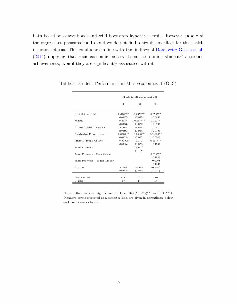
both based on conventional and wild bootstrap hypothesis tests. However, in any of

the regressions presented in Table 4 we do not find a significant effect for the health

insurance status. This results are in line with the findings of Danilowicz-Gosele et al.

(2014) implying that socio-economic factors do not determine students’ academic

achievements, even if they are significantly associated with it.

Table 3: Student Performance in Microeconomics II (OLS)

Grade in Microeconomics II

(1) (2) (3)

High School GPA 0.656*** 0.635*** 0.653***

(0.067) (0.065) (0.066)

Female -0.218** -0.215*** -0.210***

(0.076) (0.072) (0.070)

Private Health Insurance 0.0628 0.0448 0.0437

(0.086) (0.084) (0.079)

Purchasing Power Index 0.00394* 0.00403* 0.00432**

(0.002) (0.002) (0.002)

Micro I: Tough Grader -0.00995 -0.0348 0.617***

(0.085) (0.078) (0.156)

Same Professor 0.489***

(0.118)

Same Professor - Easy Grader 0.898***

(0.184)

Same Professor - Tough Grader -0.0208

(0.123)

Constant 0.0909 -0.198 -0.548*

(0.253) (0.292) (0.311)

Observations 1230 1230 1230

Cluster 17 17 17

Notes: Stars indicate significance levels at 10%(*), 5%(**) and 1%(***).

Standard errors clustered at a semester level are given in parentheses below

each coefficient estimate.

17

Table 4: Student Performance in Microeconomics II (IV) (Second Stage)

Second stageGrade in Microeconomics II

(1) (2) (3)

High School GPA 0.614*** 0.604*** 0.647***(0.061) (0.063) (0.063)[0.000] [0.000] [0.000]

Female -0.172* -0.180** -0.183***(0.088) (0.083) (0.067)[0.160] [0.200] [0.080]

Private Health Insurance 0.0570 0.0412 0.0404(0.090) (0.086) (0.077)[0.560] [0.640] [0.600]

Purchasing Power Index 0.00221 0.00274* 0.00371**(0.002) (0.002) (0.002)[0.280] [0.120] [0.080]

Micro I: Tough Grader 0.453*** 0.311** 1.385***(0.114) (0.145) (0.355)[0.000] [0.080] [0.000]

Same Professor 0.469***(0.123)[0.000]

Same Professor - Easy Grader 1.225***(0.243)[0.000]

Same Professor - Tough Grader -0.458**(0.207)[0.040]

Constant 0.132 -0.155 -0.812***(0.243) (0.278) (0.309)[0.440] [0.400] [0.080]

Observations 1230 1230 1230Cluster 17 17 17Kleibergen-Paap Wald F stat 230.162 172.419 244.436Hansens J statistic 4.619 2.135 1.382Hansen p-value 0.099 0.344 0.501


18

Table 5: Student Performance in Microeconomics II (IV) (First Stage)

First StageTough Graders

(1) (2) (3)

High School GPA 0.0829*** 0.0819*** 0.00388(0.026) (0.025) (0.016)[0.040] [0.040] [0.880]

Female -0.0881** -0.0876** -0.0338*(0.036) (0.036) (0.017)[0.120] [0.120] [0.240]

Private Health Insurance 0.00924 0.00893 -0.00262(0.025) (0.025) (0.013)[0.480] [0.520] [0.960]

Purchasing Power Index 0.00356*** 0.00357*** 0.000713(0.001) (0.001) (0.001)[0.000] [0.000] [0.120]

Course Assignment of Prof. 1 0.0881 0.0784 0.0927**(0.086) (0.085) (0.036)[0.520] [0.600] [0.080]

Course Assignment of Prof. 2 0.612*** 0.605*** 0.244***(0.046) (0.048) (0.028)[0.000] [0.000] [0.000]

Course Assignment of Prof. 3 0.643*** 0.627*** 0.0970**(0.047) (0.054) (0.044)[0.000] [0.000] [0.080]

Same Professor 0.033(0.042)[0.560]

Same Professor - Easy Grader -0.441***(0.046)[0.040]

Same Professor - Tough Grader 0.530***(0.061)[0.000]

Constant -0.150 -0.166* 0.304***(0.095) (0.093) (0.071)[0.200] [0.160] [0.000]

Observations 1230 1230 1230Cluster 17 17 17F first-stage 175 199 56646


19

4.3 Public Finance

The second subsequent course we analyze is the Public Finance course. The OLS

estimation results can be found in Table 6. Tables 7 and 8 report two-stage least squares

estimates for our outcome variable across two different specifications. Instrumentation

is strong and the results have a valid causal interpretation, as indicated by the first-

stage F-statistic and Kleibergen-Paap rk Wald F-statistic. Hansen’s J statistic is far

from rejection of its null, implying the validity of our instrument set.

Here again, we have a strong ex ante expectation that the grade obtained in Microe-

conomics I can be used as a predictor for student’s performance in the Public Finance

class. In the first specification, where we do not control for the effect of having the

same professor in both analyzed courses, we find a highly significant but, surprisingly,

negative effect of the Tough Graders. This conclusion has to be qualified to some extent,

since the wild bootstrap p-value for the Tough Graders is insignificant. This negative

effect becomes smaller once the control variable for having the same professor in both

courses is included.

Both coefficients, Tough Graders and Same Professor are highly significant in the

last specification, both based on conventional and wild bootstrap hypothesis tests. In

this case, the interpretation is a little bit different than in the case of Microeconomics

II, since there is only one professor assigned to teach this course. In order to understand

the obtained results, we need to take into account that the professor assigned to teach

the Public Finance course is the one who gives the worst grades in Microeconomics I and

thus a Tough Grader. Hence, the students who wrote their both exams, Microeconomics

I and Public Finance, with the same professor are slightly better of than those students

who took their Microeconomics I exam with one of the Easy Graders.

In contrast to the results found for Microeconomics II, the worst off are now stu-

dents who have their Microeconomics I grade from one of the other two Tough Graders.

A reason for the partly inconsistent results may be that, although both courses are

strongly related to Microeconomics I, the Public Finance course is less mathematical

and has a different examination style than Microeconomics II. In Microeconomics I and

Microeconomics II students complete exam problems that are either similar to the mul-

tiple choice question type (true/false) or graded on the basis of the final result (fill-ins).

However, exam problems in Public Finance include essay questions and calculations

which gives professors more freedom in grading their students. For this reasons, we did

not expect to find such a strong effect of having the same professor in both courses.

20

This finding suggests that there are differences in professors’ characteristics, not

only between the Easy Graders and the Tough Graders, but also within those groups.

In order to analyze this, we create two sub-samples: the first one includes students who

wrote their Microeconomics I exam either with the professor who gives the worst grades

(Professor 1) or with the professor who gives the best grades (Professor 5). The second

sub-sample consists of students who took their Microeconomics I exam again with the

toughest grader (Professor 1) or with the second toughest grader (Professor 2). The

results of estimating the effect of a single professor on the grade in Public Finance exam

can be found in Tables 9 and 10. The baseline category is now represented by Professor

1. For both professors, Professor 2 and Professor 5, we find highly significant and

negative effect on student’s performance in Public Finance. According to this result,

having a tough professor in Microeconomics I does not always positively affect student’s

later performance in follow-on courses. Here, a student who took her Microeconomics I

exam with a professor who “gives out” grades is better off than a student with the second

toughest grader. On the one hand, it looks like, some of the Tough Graders teach better

and demand higher performance from their students, others just give lower grades.

On the other hand, Easy Graders do not always “only” inflate grades. Furthermore,

looking at some other follow-on courses suggests that students benefit from having an

Easy Grader in less theoretical courses where mathematical skills are not that essential

and examinations thus require less calculations.

In addition, we find the expected highly significant and positive effect of the high

school leaving degree on students’ grade in Public Finance exam. Since the Public

Finance course is a less mathematical one, we do not find a significant effect for female,

which is again consistent with our previous argumentation about prevalent gender gap

in mathematics. The effect of student’s health insurance type is now highly significant

and positive, which can be explained by the differences in students composition between

Microeconomics and Public Finance. Microeconomics courses are mandatory for many

students enrolled at the faculty of economic sciences. Public Finance, on the contrary,

is completed mostly by the students from economics, who in contrast to their business

colleagues, are less known for being fast climbers which in turn can relate to their

wealthy family status.

21

Table 6: Student Performance in Public Finance (OLS)

Grade in Public Finance

(1) (2)

High School GPA 0.594*** 0.576***(0.067) (0.070)

Female 0.0210 0.0190(0.075) (0.073)

Private Health Insurance 0.251*** 0.273***(0.057) (0.057)

Purchasing Power Index 0.00330 0.00287(0.003) (0.003)

Micro I: Tough Grader -0.0931 -0.690***(0.103) (0.108)

Same Professor 0.732***(0.138)

Constant 0.404 0.487(0.317) (0.349)

Observations 961 961Cluster 14 14

Notes: Stars indicate significance levels at 10%(*), 5%(**) and 1%(***).Standard errors clustered at a semester level are given in parentheses beloweach coefficient estimate.

Table 7: Student Performance in Public Finance (IV) (Second Stage)

Second stageGrade in Public Finance

(1) (2)

High School GPA 0.671*** 0.576***(0.057) (0.068)[0.000] [0.000]

Female -0.0757 0.0178(0.071) (0.070)[0.240] [0.920]

Private Health Insurance 0.271*** 0.274***(0.070) (0.055)[0.000] [0.000]

Purchasing Power Index 0.00645** 0.00290(0.003) (0.002)[0.080] [0.120]

Micro I: Tough Grader -0.926*** -0.723***(0.329) (0.110)[0.120] [0.040]

Same Professor 0.761***(0.142)[0.000]

Constant 0.313 0.490(0.295) (0.337)[0.400] [0.280]

Observations 961 961Cluster 14 14Kleibergen-Paap Wald F stat 208.172 3468.381Hansens J statistic 2.365 2.652Hansen p-value 0.306 0.266


22

Table 8: Student Performance in Public Finance (IV) (First Stage)

First StageTough Graders

(1) (2)

High School GPA 0.0970*** 0.0124(0.024) (0.008)[0.000] [0.160]

Female -0.108** -0.0129*(0.046) (0.007)[0.040] [0.080]

Private Health Insurance 0.0135 0.0291(0.037) (0.020)[0.840] [0.120]

Purchasing Power Index 0.00446*** 0.00132*(0.001) (0.001)[0.000] [0.120]

Course Assignment of Prof. 1 0.109 0.0139(0.104) (0.019)[0.280] [0.440]

Course Assignment of Prof. 2 0.659*** 0.925***(0.047) (0.042)[0.000] [0.000]

Course Assignment of Prof. 3 0.684*** 0.705***(0.043) (0.009)[0.000] [0.000]

Same Professor 0.936***(0.040)[0.000]

Constant -0.296** -0.120(0.101) (0.068)[0.040] [0.120]

Observations 961 961Cluster 14 14F first- stage 158 20274


23

Table 9: Student Performance in Public Finance (IV) - Comparison (Second Stage)

Second stageGrade in Public Finance

Professor 5 Professor 2

High School GPA 0.523*** 0.616***(0.065) (0.093)[0.000] [0.000]

Female 0.104 -0.0698(0.067) (0.075)[0.080] [0.320]

Private Health Insurance 0.291*** 0.385***(0.072) (0.097)[0.000] [0.000]

Purchasing Power Index 0.00260 0.00119(0.003) (0.003)[0.520] [0.840]

Micro I: Professor 5 -0.396***(0.147)[0.040]

Micro I: Professor 2 -0.522***(0.137)[0.040]

Constant 0.836* 0.601(0.459) (0.474)[0.120] [0.160]

Observations 697 410Cluster 13 13Kleibergen-Paap Wald F stat 69.702 206.523Hansens J statistic 0.000 0.000


24

Table 10: Student Performance in Public Finance (IV) - Comparison (First Stage)

First StageProfessor 5 Professor 2

High School GPA -0.101*** 0.00980(0.031) (0.014)[0.080] [1.000]

Female 0.129** 0.0146(0.059) (0.015)[0.120] [0.640]

Private Health Insurance -0.0199 0.0526(0.051) (0.039)[0.680] [0.280]

Purchasing Power Index -0.00442*** 0.00203(0.001) (0.001)[0.040] [0.200]

Course Assignment of Prof. 5 0.329***(0.394)[0.000]

Course Assignment of Prof. 2 0.917***(0.064)[0.000]

Constant 1.062*** -0.208(0.136) (0.149)[0.000] [0.400]

Observations 697 410Cluster 13 13F first- stage 26 747


5 Discussion

In recent years a great number of studies on higher education have emphasized fac-

tors that might influence students’ performance. While most of those studies focus on

students’ characteristics such as previous academic performance, age or socio-economic

status, less attention has been paid to the impact of professors’ characteristics or pro-

fessors’ grading.

Therefore in this paper, we analyze the impact of professors’ characteristics on

students’ achievement using data from almost 3,000 students from Gottingen University.

By looking at three courses at the Faculty of Economic Sciences, we first capture the

professor’s effect from the mandatory first-year course (Microeconomics I) and then

analyze its effect on student’s performance in follow-on courses (Microeconomics II and

Public Finance). Two main results emerge from our analysis. Firstly, we find that

it matters, for student’s later university performance in micro-related courses, which

professor was teaching and giving the Microeconomics I exam. Our results suggest

that students can benefit from having a tough or an easy grader in a fundamental

25

course, with the effects depending on the student’s prior academic performance and

design of the follow-on course, in particular the mathematical content of the course

and the resulting examination form. Secondly, we show that the effect of having the

same professor in Microeconomics I and in one of the two analyzed follow-on courses

is significant and highly relevant. Thus, students benefit much more from the familiar

teaching practices and the familiar examination style. In some cases, this positive effect

can even compensate or partially compensate for the negative professor’s effect from

Microeconomics I course.

From the consideration of the above results two questions arise: How can we explain

the arising differences in grading? and Do the Tough Graders indeed prepare students

for more rigorous mathematical and analytical standards by teaching something differ-

ent than their easy grading colleagues? In order to answer the first question, we should

consider if there are, besides the grading, other substantial differences between both

professor’s groups included in our analysis. When looking at the groups individually,

professors assigned to the Easy Graders are of higher age, have been employed longer

at a university and do less research than their younger colleagues. Together, our results

and these facts lead us to hypothesize that professor’s age and teaching experience may

be, above certain threshold, positively associated with students’ grades. Older profes-

sors very often exude grandfather’s mildness and thus have more understanding for the

students. Another explanation for this result may stem from the fact that the longer a

professor was teaching the same subject, the easier he is to predict.

Furthermore, we can think about other factors, besides individual characteristics of

the teaching body, that potentially affect the grades and may differ between professors.

One of them is the class size. Since all professors structure the course in the same

way, offering lecture and tutorials on a weekly basis should not be an issue. Also the

credentials of the faculty teaching team should not determine our results, since we do

not observe striking differences in education level between the assigned professors and

their assistants. In addition, all professors included in our data set have very similar

status, implying that none of them are in a position of having to earn good evaluations

in order to be able to keep their job. Nonetheless, some of the professors may generally

tend to keep the students happy by giving them good, possibly inflated, grades. In

particular, those professors, who are close to retire, are less stringent since they want

to leave a good impression.

From the students’ point of view, the benefit of having an Easy Grader or a Tough

Grader in Microeconomics I depends to a great extent on the student’s course choices

26

and her timing. If grades were the only aim, students may act strategically by taking

advantage of the mentioned differences, which will result in postponing the exams until

the desired professor is offering the class or in attending only carefully-selected courses.

Our analysis shows that the obtained effects are quite meaningful. All else being equal,

having a certain professor in Microeconomics I is associated with an improvement of

the expected grade in a follow-on course by up to 1.385 grades. Therefore, making

smart strategic choices about study pathways may lead to a considerable improvement

of the final grade.

From the above results we conclude that there is much variability in grading not

only between universities or faculties, but also from one professor to the next and be-

tween courses within a field. The increasing diversity especially within higher education

system is valuable but comes at the expense of transparency in grading policies. Al-

though grades are used to motivate students and to report the quality of student’s

performance for employers, researchers and politicians consistently raise arguments in

favor of abandoning grades and rather encouraging students to pursue more than a

perfect transcript.

27

References

Babcock, P. and Marks, M. (2011). The falling time cost of college: Evidence from

half a century of time use data. The Review of Economics and Statistics, MIT Press,

93(2):468–478.

Bar, T., Kadiyali, V., and Zussman, A. (2009). Grade information and grade inflation:

The cornell experiment. Journal of Economic Perspectives, 23(3):93–108.

Baum, C., Schaffer, M., and Stillman, S. (2007). Enhanced routines for instrumental

variables/gmm estimation and testing. CERT Discussion Papers 0706, Centre for

Economic Reform and Transformation, Heriot Watt University.

Bettinger, E. P. and Long, B. T. (2005). Do faculty serve as role models? The impact

of instructor gender on female students. American Economic Review, 95(2):152–157.

Birnbaum, R. (1977). Factors Related to University Grade Inflation. The Journal of

Higher Education, 48(5):519–539.

Cameron, A. C., Gelbach, J. B., and Miller, D. L. (2008). Bootstrap-based im-

provements for inference with clustered errors. Review of Economics and Statistics,

90(3):417–427.

Cameron, A. C. and Trivedi, P. K. (2010). Microeconometrics Using Stata. Stata Press,

College Station, Texas.

Carrell, S. E., Page, M. E., and West, J. E. (2010). Sex and science: How professor gen-

der perpetuates the gender gap. The Quarterly Journal of Economics, 125(3):1101–

1144.

Clotfelter, C. T., Ladd, H. F., and Vigdor, J. L. (2007). Teacher credentials and

student achievement: Longitudinal analysis with student fixed effects. Economics of

Education Review, 26(6):673 – 682. Economics of Education: Major Contributions

and Future Directions - The Dijon Papers.

Danilowicz-Gosele, K., Meya, J., Schwager, R., and Suntheim, K. (2014). Determinants

of student success at university. Gottingen.

De Paola, M. (2009). Does teacher quality affect student performance? Evidence from

an italian university. Bulletin of Economic Research, 61(4):353–377.

28

Eiszler, C. F. (2002). College students’ evaluations of teaching and grade inflation.

Research in Higher Education, 43(4):483–501.

Ellison, G. and Swanson, A. (2010). The gender gap in secondary school mathematics

at high achievement levels: Evidence from the american mathematics competitions.

Journal of Economic Perspectives, 24(2):109–28.

Finkenstadt, V. and Keßler, T. (2012). Die soziookonomische Struktur der PKV-

Versicherten: Ergebnisse der Einkommens- und Verbrauchsstichprobe 2008. WIP

Discussion Paper, No. 3/2012, Koln.

Hoffmann, F. and Oreopoulos, P. (2009). A professor like me: The influence of instructor

gender on college achievement. The Journal of Human Resources, 44(2):479–494.

Johnson, V. E. (2003). Grade Inflation: A Crisis in College Education. New York:

Springer.

Kena, G., Musu-Gillette, L., Robinson, J., Wang, X., Rathbun, A., Zhang, J.,

Wilkinson-Flicker, S., Barmer, A., and Dunlop Velez, E. (2015). The condition of

education 2015 (nces 2015-144). U.S. Department of Education, National Center for

Education Statistics. Washington, DC.

Krautmann, A. C. and Sander, W. (1999). Grades and student evaluations of teachers.

Economics of Education Review, 18(1):59 – 63.

Miles, D. A. and Sparks, W. (2013). Examining social media and higher education:

An empirical study on rate my professors.com and its impact on college students.

International Journal of Economy, Management and Social Sciences, 2(7):513–524.

Nelson, J. P. and Lynch, K. A. (1984). Grade inflation, real income, simultaneity, and

teaching evaluations. The Journal of Economic Education, 15(1):21–37.

Neumark, D. and Gardecki, R. (1998). Women helping women? Role model and

mentoring effects on female ph.d. students in economics. The Journal of Human

Resources, 33(1):220–246.

Ost, B. (2010). The role of peers and grades in determining major persistence in the

sciences. Economics of Education Review, 29(6):923 – 934.

29

Prather, James E., G. S. and Kodras, J. E. (1979). A Longitudinal Study of Grades in

144 Undergraduate Courses. Research in Higher Education, 10(1):11–24.

Pressman, S. (2007). The economics of grade inflation. Challenge, 50(5):93–102.

Rivkin, S. G., Hanushek, E. A., and Kain, J. F. (2005). Teachers, schools, and academic

achievement. Econometrica, 73(2):417–458.

Rojstaczer, S. and Healy, C. (2010). Grading in American Colleges and Universities.

Teachers College Record, 4.

Sabot, R. and Wakeman-Linn, J. (1991). Grade inflation and course choice. Journal of

Economic Perspectives, 5(1):159–170.

Statistisches Bundesamt (2009). Bildungsstand der Bevolkerung: Ausgabe 2009, Wies-

baden.

Stratton, R. W., Myers, S. C., and King, R. H. (1994). Faculty behavior, grades, and

student evaluations. The Journal of Economic Education, 25(1):5–15.

Xie, Y. and Shauman, K. A. (2003). Women in science: Career processes and outcomes.

Harvard University Press.

30

Date post:	12-Dec-2021
Category:	Documents
Upload:	others
View:	2 times
Download:	0 times

“A” is the Aim? - GWDG

Documents