A Jackknife-Type Estimator for Portfolio Revision∗

Roland Fuss† Felix Miebs‡ Fabian Trubenbach§

October 30, 2011

Abstract

This article proposes a novel approach to optimal portfolio revision. The currentliterature on portfolio optimization uses a somewhat naive approach, where portfolioweights are always completely revised after a predefined fixed period. However,one shortcoming of this procedure is that it ignores parameter uncertainty in theestimated portfolio weights, as well as the biasedness of the in-sample portfoliomean and variance as estimates of the expected portfolio return and out-of-samplevariance. To rectify this problem, we propose a Jackknife procedure to determinethe optimal revision intensity, i.e., the percent of wealth that should be shifted to thenew, in-sample optimal portfolio. We find that our approach leads to highly stableportfolio allocations over time, and can significantly reduce the turnover of severalwell established portfolio strategies. Moreover, the observed turnover reductionslead to statistically and economically significant performance gains in the presenceof transaction costs.

JEL Classification: G11Key words: Portfolio optimization, Portfolio revision, Jackknife, Transaction costs

∗Comments are welcome.†EBS Business School, Department of Finance, Accounting and Real Estate, Gustav-Stresemann-Ring

3, 65189 Wiesbaden, Germany, roland.fuess@ebs.edu.‡EBS Business School, Department of Finance, Accounting and Real Estate, Gustav-Stresemann-Ring

3, 65189 Wiesbaden, Germany, felix.miebs@ebs.edu.§EBS Business School, Department of Finance, Accounting and Real Estate, Gustav-Stresemann-Ring

3, 65189 Wiesbaden, Germany, fabian.truebenbach@ebs.edu.

1 Introduction

Despite the theoretical appeal of Markowitz’s (1952) mean-variance paradigm, it has three

prominent criticisms. First, the mean-variance algorithm is believed to yield highly un-

balanced allocations (see, e.g., Green and Hollifield (1992) as well as Black and Litterman

(1992)). Second, the impact of even small changes in the input parameters can cause dra-

matic shifts in the derived allocations (see, e.g., Best and Grauer (1991), Chopra (1993),

and Chopra and Ziemba (1993)). Third, its repeated use over time leads to compara-

tively unstable allocations, resulting in higher turnovers (see Chopra et al. (1993)). The

literature contains several potential remedies for the first two issues; relatively little at-

tention, however, has focused on the immense turnover of mean-variance portfolios and

the associated question of portfolio revisions.

In this paper, we tackle the question of optimal portfolio revision. Specifically,

we explore when and how much investors should consider shifting from their current

portfolios to new in-sample optimal portfolios. We assess this question based on the

established rolling sample approach to portfolio optimization, in which investors typically

revise their entire portfolios after a predefined but arbitrarily chosen time period. The

investor then holds the new optimal portfolio, which is optimized over the corresponding

new in-sample period. This revision policy appears intuitive, because the new portfolio

dominates the old one in terms of in-sample mean-variance efficiency. The fixed portfolio

revision frequency is also in line with the myopic nature of the Markowitz framework.

However, a significant shortcoming of this approach is that it is based on in-sample

mean-variance efficiency. As Kan and Zhou (2007), Siegel and Woodgate (2007), and

Basak et al. (2009) have shown, in-sample portfolio mean and variance are not consistent

estimators of expected out-of-sample return and variance because of the potential for

estimation errors. Specifically, these authors note that in-sample portfolio returns that

are optimized in the presence of estimation errors tend to overestimate expected out-of-

sample returns. In-sample variance, on the other hand, tends to underestimate expected

1

out-of-sample variance.1

As a result of this in-sample overoptimism, investors may be reluctant to revise their

portfolios without a concurrent increase in expected out-of-sample performance. To deal

with this issue, we base our revision policy on the expected out-of-sample performance of

a portfolio, which we consider as the natural investor objective for portfolio revisions.

We use Basak et al.’s (2009) Jackknife procedure to obtain consistent estimates of the

expected out-of-sample portfolio performance of the investor’s current portfolio versus the

new, in-sample optimal portfolio. We then need to determine what percentage to allocate

to the new portfolio. We provide an analytic expression for the optimal revision intensity,

and evaluate our revision policy by applying it to various minimum-variance portfolio

strategies across five datasets. We could also apply our portfolio revision framework to

mean-variance portfolios, but our focus is solely on minimum-variance portfolios because

broad empirical evidence has shown that they perform better out-of-sample (see Jobson

and Korkie (1981) as well as Jagannathan and Ma (2003), among others).

We assess the performance of our revision policy on simulated datasets as well as on

five empirical datasets. For both simulation and empirical analysis, we achieve compara-

ble portfolio performance in terms of the Sharpe ratio and the certainty equivalent return,

suggesting our revision policy can lead to substantially lower turnovers than policies with

fixed revision frequencies. Empirically, we observe that our revision policy reduces aver-

age monthly turnovers by up to 77.6%, with average reductions ranging from 23.3% for

the Ledoit and Wolf (2004a) to 38.9% for the shortsale constrained minimum-variance

portfolio.

If we include trading costs in our analysis, we observe that, because of the sizable

turnover reduction, our portfolio revision policy yields economically and statistically sig-

nificant performance gains. Assuming proportional round-trip transaction costs of 1%,

1Kan and Zhou (2007) as well as Siegel and Woodgate (2007) demonstrate that this in-sample overopti-mism is inversely related to the number of observations available to estimate the input parameters forthe optimization parameters. It also increases with the number of assets.

2

we find that, compared to monthly or annual portfolio revision, investors with a risk aver-

sion of five would theoretically be willing to pay an annual management fee of between

101 and 168 basis points (bps). Our results are especially strong for datasets with larger

asset universes, where the higher ratio of number of assets to number of time periods

(N/T ) increases the estimation error of the covariance matrix estimates. This creates

more unbalanced allocations, along with higher turnover.

There are two main strands of literature on portfolio revisions of mean-variance

efficient portfolios: dynamic revision strategies (e.g. Chen et al. (1971), Kamin (1975),

and Leland (1999)), and retrospectively determined optimal revision frequencies or ranges

(e.g. Arnott and Lovell (1993), Plaxco and Arnott (2002), and Tokat and Wicas (2007)).

Dynamic revision strategies are generally complex, computationally intensive, and

thus somewhat limited to small investment universes (see Donhue and Yip (2003)). No-

tably, the Markowitz and van Dijk (2003) as well as Kritzman et al. (2009) approxima-

tions represent scalable alternatives to dynamic revision strategies. However, they remain

a heuristic approximation to the underlying dynamic program. The heuristic nature of

these approximations is also reflected in the retrospectively determined optimal revision

frequencies or ranges. The revision frequencies do not follow any objective optimality

criteria, and may thus be regarded as heuristic.

In addition to the two major approaches to portfolio revisions, the literature contains

two minor approaches: the imposition of turnover constraints (Schreiner (1980)), and the

use of statistical process control charts for determining optimal portfolio revisions (Golos-

noy (2009)). Both approaches require threshold values to trigger the revision process,

however, which renders the results highly sensitive to the chosen threshold. Furthermore,

all of the approaches mentioned thus far neglect the impact of estimation errors and any

corresponding in-sample overoptimism on the revision decision.

Our paper contributes to the existing literature in three ways. First, our approach

represents a new method to overcoming the problem of optimal portfolio revision by

3

focusing on the (consistently estimated) expected out-of-sample performance of the revised

portfolio, which we regard as the natural objective for revision. Accordingly, our approach

takes into account the problem of estimation errors and in-sample overoptimism. Second,

we derive our estimator by optimizing expected out-of-sample portfolio performance. This

represents an exact solution to the revision problem, rather than a heuristic one. By

focusing on the expected out-of-sample performance of the revised portfolio, our approach

is easily scalable and computationally inexpensive, even for large investment universes.

Third, our estimator gives a purely data-driven solution to the portfolio revision problem.

It requires neither calibration nor a threshold value. It is thus easily implementable,

and of interest for practical applications. The remainder of this paper is organized as

follows. Section 2 describes our framework for optimal portfolio revision, reviews the

various minimum-variance portfolio strategies that we use to evaluate the profitability of

our policy, and outlines our performance evaluation procedure. Section 3 discusses our

proposed revision policy using simulated data, while section 4 explores its performance

on empirical datasets. Section 5 gives our conclusions.

2 Methodology

2.1 Optimal Portfolio Revision Policy

Throughout this paper, we consider the typical myopic minimum-variance portfolio op-

timization problem. The investor’s objective is to minimize w′Σw, where w denotes a

column vector of optimal portfolio weights, and Σ represents the population covariance

matrix. Because Σ is not observable, we use an estimate based on sample information,

denoted by S. The sample estimate of the portfolio variance is thus w′Sw, where w

represents the sample estimate of w.

In the traditional rolling sample approach to portfolio optimization, investors de-

termine wt at the end of each period t using the sample information from the previous

4

using τ months. The portfolio weights are held constant over the consecutive period,

t + 1. At the end of the period, the investor receives the corresponding out-of-sample

return w′tRt+1, where Rt+1 denotes the cross-section of excess returns in period t + 1.

The investor then determines the new optimal portfolio weights, wt+1, conditional on the

sample information of the new estimation period, which ranges from t + 2 − τ to t + 1.

Finally, investors completely revise their portfolio weights to the new portfolio weights,

wt+1, since the old portfolio weights, wt, are no longer efficient conditional on the new

in-sample information. This procedure is then repeated over the entire sample period.

Note that Kan and Zhou (2007), Siegel and Woodgate (2007), and Basak et al.

(2009) show that the in-sample variance of a portfolio is not a consistent estimator of

expected out-of-sample variance. This intuitively appears to be the quantity of interest

when investors revise their minimum-variance portfolios.

Basak et al. (2009) particularly demonstrate that the in-sample variance of a portfo-

lio can suffer from overoptimism and systematically underestimate out-of-sample variance.

Hence, because the new in-sample optimal portfolio weights do not necessarily yield lower

expected out-of-sample variance, investors may not be better off revising their weights

from the previous period to the current period. Rather, it may be more advantageous

to hold a combination of both weight estimates, because this could yield diversification

benefits if the expected out-of-sample variances are not perfectly correlated. Moreover,

holding the weights of the previous period constant may even yield a lower expected

out-of-sample variance than shifting them toward the new ones.

Aside from the expected out-of-sample variance, managing the turnover resulting

from a portfolio revision is crucial for the practical implementation of a portfolio strategy.

Typically, higher turnover hampers implementation, and can adversely affect portfolio

performance in the presence of trading costs. Hence, investors will generally prefer less

frequent revisions of portfolio weights due to a decrease in turnover.

Aside from the expected out-of-sample variance, the turnover resulting from revis-

5

ing a portfolio is crucial when it comes to the practical implementation of a portfolio

strategy. Typically, a higher turnover hampers practical implementation and adversely

affects portfolio performance in the presence of trading costs. Hence, associated with a

decrease in turnover, less frequent revision of portfolio weights will generally be preferred

by investors.

2.1.1 Portfolio revision in a two-period setting

For the sake of simplicity, we first describe our portfolio revision policy in a two-

period setting. Our objective is to minimize the expected out-of-sample portfolio vari-

ance, V ar(wRev

′t Rt+1

), where wRevt is the convex combination of the estimated port-

folio weights of the current and previous period, denoted by wt and wt−1, respec-

tively. The portfolio weights of our proposed revision policy in period t are obtained

by wRevt = αwt−1 + (1 − α)wt, where α is the fraction of wealth that the investor keeps

in the portfolio weights from the previous period, wt−1. We can express the quantity of

interest (the expected out-of-sample portfolio variance), as follows:

minαV ar

(wRev

′

t Rt+1

)= V ar

(αw′t−1Rt+1 + (1− α)w′tRt+1

). (1)

The first and second derivatives of V ar(wRev

′t Rt+1

)yield:

V ar′(wRev

′

t Rt+1

)= αV ar(w′t−1Rt+1 − w′tRt+1)− V ar(w′tRt+1)

+Cov(w′t−1Rt+1, w′tRt+1), (2)

V ar′′(wRev

′

t Rt+1

)= V ar(w′t−1Rt+1 − w′tRt+1). (3)

Setting V ar′(wRev

′t Rt+1

)= 0 and solving for α yields the optimal combination intensity,

α∗, which minimizes the expected out-of-sample portfolio variance as follows:

α∗ =V ar(w′tRt+1)− Cov(w′t−1Rt+1, w

′tRt+1)

V ar(w′t−1Rt+1 − w′tRt+1). (4)

6

Because (3) is positive everywhere, the expression in (4) is verified as a global minimum for

the expected out-of-sample variance. However, note that α∗ is not a bona fide estimator,

since it depends on the unobservable quantities V ar(w′tRt+1), Cov(w′t−1Rt+1, w′tRt+1), and

V ar(w′t−1Rt+1 − w′tRt+1). Hence, we need to estimate the quantities in (4) consistently.

To do this, we use Basak et al.’s (2009) Jackknife-type estimator of the expected

out-of-sample portfolio return moments. Following this methodology, we first drop the

i-th observation from the in-sample period and compute the resulting covariance matrix

based on the remaining τ−1 returns, denoted by St,i. Next, we determine the correspond-

ing optimal portfolio weights, denoted by wt,i. Finally, we compute the Jackknife return,

RJKt,i , that would have been achieved from holding wt,i in period i, given by w′t,iRi. Re-

peating the aforementioned process for all i = {1, .., τ} leaves us with τ Jackknife returns{RJKt,1 , R

JKt,2 , · · · , RJK

t,τ

}.

Based on the underlying Jackknife assumption that returns on risky assets are iden-

tically and independently distributed over time, Basak et al. (2009) show that the dis-

tribution of RJKt,i follows the same distribution as w′tRt+1. The sample variance based on

the τ Jackknife returns thus represents a natural estimator of the out-of-sample variance,

V ar(w′tRt+1), denoted by:2

V ARJK

(w′tRt+1) =1

τ

τ∑i=1

(RJKt,i − µwt

)2, with (5)

µwt =1

τ

τ∑i=1

RJKt,i . (6)

Note that when we estimate the remaining quantities in Equation (4),

Cov(w′t−1Rt+1, w′tRt+1) and V ar(w′t−1Rt+1 − w′tRt+1), we find only τ − 1 overlap-

ping Jackknife returns available for computation.

This is attributable to the use of the rolling sample procedure. The intuition of this

procedure is that only the last τ observations are relevant for determining the quantity of

2See Basak et al. (2009) for further discussion of this point.

7

interest. We thus need to compute Cov(w′t−1Rt+1, w′tRt+1) and V ar(w′t−1Rt+1 − w′tRt+1)

based on the same observations (the most recent τ returns).

In period t the Jackknife return for wt−1 is missing in the last period of the sample

used to estimate wt. To overcome this problem, we compute the out-of-sample return for

wt−1 for the missing observation, which is w′t−1Rt. From this, we can obtain a vector of ap-

proximate Jackknife returns3 for wt−1, consisting of{w′t−1Rt, R

JKt−1,1, R

JKt−1,2, · · · , RJK

t−1,τ−1}

.

Because the sequence of all Jackknife returns for wt−1 has the same distribution as w′t−1Rt

using it does not alter the distribution. It further enables us to obtain consistent estimates

of Cov(w′t−1Rt+1, w′tRt+1) and V ar(w′t−1Rt+1 − w′tRt+1) based on the last τ observations.

We can thus estimate Cov(w′t−1Rt+1, w′tRt+1) as:

CovJK (

w′t−1Rt+1, w′tRt+1

)=

1

τ

((w′t−1R1 − µwt−1

) (RJKt,1 − µwt

))+

1τ

∑τi=2

(RJKt−1,i − µwt−1

) (RJKt,i − µwt

), with (7)

µwt−1 = 1τ

(w′t−1R1 +

∑τi=2R

JKt−1,i

)and µwt as defined in (6),

and V ar(w′t−1Rt+1 − w′tRt+1) as:

V arJK (

w′t−1Rt+1 − w′tRt+1

)=

1

τ

((w′t−1R1 −RJK

t,1

)− µwt−1−wt

)2+

1τ

∑τi=2

((RJKt−1,i −RJK

t,i

)− µwt−1−wt

)2, with (8)

µwt−1−wt = 1τ

((w′t−1R1 −RJK

t,1

)+∑τ

i=2RJKt−1,i −RJK

t,i ,),

which finally allows us to estimate α∗ as:

a∗ =V ar

JK(w′tRt+1)− Cov

JK(w′t−1Rt+1, w

′tRt+1)

V arJK

(w′t−1Rt+1 − w′tRt+1). (9)

Naturally, a∗ may lie outside the desired range between 0 (the portfolio is totally revised

3The term ”approximate Jackknife returns” accounts for the mixture of out-of-sample returns and Jack-knife returns in the vector.

8

to the new portfolio weights) and 1 (the portfolio is not revised at all). To ensure that

a∗ lies within the desired interval, we cut off values that lie outside the [0, 1] interval, so

that:

a = max [0,min (1, a∗)] . (10)

2.1.2 Portfolio revision in a multi-period setting

It is straightforward to extend the revision scheme of the two-period case to a multi-period

setting. In a multi-period setting, the weights of the previous period are already a convex

combination of those from the preceding t− 1 periods. However, two minor adjustments

are necessary. First, we must change the notation of the old portfolio weights from the

previous period from wt−1 to wRevt−1 to account for the fact that wRevt−1 is not fully determined

by wt−1. In other words, the revised portfolio weights of the last period have not been or

have only been partially revised to the portfolio weight estimate wt−1.

Second, we must track the solution to the out-of-sample variance minimization prob-

lem in (1) over time, to determine both the share of less recent portfolio weight estimates

of wRevt−1 and the corresponding determination of the expected out-of-sample variance. We

can thus describe investors’ revision decisions in each period t by the following minimiza-

tion problem:

minαt

V ar(wRev

′

t Rt+1

)= V ar

(αtw

Rev′

t−1 Rt+1 + (1− αt)w′tRt+1

). (11)

Similarly to the two-period case, this solves as:

α∗t =V ar(w′tRt+1)− Cov(wRev

′t−1 Rt+1, w

′tRt+1)

V ar(wRev′

t−1 Rt+1 − w′tRt+1). (12)

Again, we face the problem that α∗t is not a bona fide estimator. Accordingly, we need to

estimate V ar(w′tRt+1), Cov(wRev′

t−1 Rt+1, w′tRt+1), and V ar(wRev

′t−1 Rt+1 − w′tRt+1). Because

9

V ar(w′tRt+1) does not differ from the two-period case, we can estimate it by using the

estimator in (5).

Estimating Cov(wRev′

t−1 Rt+1, w′tRt+1) and V ar(wRev

′t−1 Rt+1− w′tRt+1), however, is more

complex. Because both quantities depend on wRevt−1 it may be a convex combination of

{wt−1, wt−2, . . . , wt−n}. We thus need to compute the expected out-of-sample variance for

wRev′

t−1 by taking all n portfolio weights into account.4

To illustrate this in practice, let rj,t denote the vector of approximate Jackknife

returns corresponding to wt, where j denotes the period for which the portfolio weights

and the corresponding Jackknife returns{RJKj,1 , R

JKj,2 , · · · , RJK

j,τ

}were initially calculated.

Whenever αt takes a value of 0, the following procedure applies to the consecutive peri-

ods: we obtain return vector rt,t, consisting of τ Jackknife returns{RJKt,1 , R

JKt,2 , · · · , RJK

t,τ

}in the first period, t. In the following period, t + 1, we obtain the new return vector,

rt+1,t+1, which again consists of τ Jackknife returns{RJKt+1,1, R

JKt+1,2, · · · , RJK

t+1,τ

}. The

previous return vector, rt,t, then becomes rt,t+1 in t + 1, indicating that it comprises

τ − 1 Jackknife returns corresponding to portfolio wt and one out-of sample return{w′tRt+1, R

JKt,1 , R

JKt,2 , · · · , RJK

t,τ−1}

. After the revision decision in t + 1, we determine the

approximate Jackknife return vector of the revised portfolio, rRevt+1 , as follows:

rRevt+1 = α1rt,t+1 + (1− α1)rt+1,t+1.

Consequently, the entries in the vector of approximate Jackknife returns rRevt+1 are given by{α1w

′tRt+1 + (1− α1)R

JKt+1,1, α1R

JKt,1 + (1− α1)R

JKt+1,2, · · · , α1R

JKt,τ−1 + (1− α1)R

JKt+1,τ

}. In

4Note that the number of portfolio weights, n, contained in wRevt−1 depends on the historical values of

{αt−1, αt−2, · · ·αt−n}. As long as none of the n alphas is equal to zero, wRevt−1 will be a convex combination

of all portfolio weights determined over the n periods. In contrast, as soon as any alpha equals zero,the portfolio weights are completely revised to the new, in-sample optimal weights, which render the oldweights and their corresponding approximate Jackknife returns obsolete.

10

the next period, the same procedure applies as follows:

rRevt+2 = α2[α1rt,t+1 + (1− α1)rt+1,t+1] + (1− α2)rt+2,t+2

= α2rRevt+1 + (1− α2)rt+2,t+2.

It is obvious that, unless the n-th αt takes a value of zero, the vector of approximate

Jackknife returns corresponding to wt is determined by:

rRevt+n = αnrRevt+n−1 + (1− αn)rt+n,t+n.

Let rRevt,i and rt,t,i denote the i-th element of the vector rRevt and rt,t, respectively.

Following the intuition of the revision scheme described above, we can then estimate

Cov(wRev′

t−1 Rt+1, w′tRt+1) as:

CovJK(wRev

′

t−1 Rt+1, w′tRt+1

)=

1

τ

τ∑i=1

(rRevt−1,i −

1

τ

τ∑i=1

rRevt−1,i

)(rt,t,i −

1

τ

τ∑i=1

rt,t,i

), (13)

and V ar(wRev′

t−1 Rt+1 − w′tRt+1) as:

V arJK(wRev

′

t−1 Rt+1 − w′tRt+1

)=

1

τ

τ∑i=1

((rRevt−1,i − rt,t,i

)− 1

τ

τ∑i=1

(rRevt−1,i − rt,t,i

))2

, (14)

which finally allows us to estimate α∗ as:

a∗ =V ar

JK(w′tRt+1)− Cov

JK(wRev

′t−1 Rt+1, w

′tRt+1)

V arJK

(wRev′

t−1 Rt+1 − w′tRt+1). (15)

Analogously to the two-period case, we trim the estimator a∗ according to Equation (10)

in order to ensure that the values lie inside the [0, 1] interval.

11

2.2 Description of Evaluated Portfolios

In this section, we briefly describe the minimum-variance portfolio strategies we use to

evaluate our proposed revision policy. The difference between the various portfolio strate-

gies is attributable to the different estimators of the variance-covariance matrix. All

portfolio weights are computed by solving the following optimization problem:

minww′Sw (16)

s.t. w′1N = 1,

where 1N denotes a vector of ones of appropriate size. The well-known solution to this

minimization problem is given by:

w = S−11N(1′NS−11N)−1, (17)

which is the sample estimate of the global minimum-variance portfolio weights. For our

analysis we focus on the most prominent covariance matrix estimators and correspond-

ing minimum-variance portfolios in the portfolio selection literature. An overview of all

portfolios is given in Table 1.

[INSERT TABLE 1 HERE]

Our selection of minimum-variance portfolios may be divided into two groups: the first is

based on a single covariance matrix estimate whereas the second is based on a combination

of two covariance matrix estimators. Within the first group of minimum-variance port-

folios, we consider three covariance matrix estimators. First, we evaluate the minimum-

variance portfolio based on the sample covariance matrix (SAMPLE) as given by:

SSample =1

τ − 1XX ′, (18)

12

where X denotes a τ×N matrix of de-meaned returns. Second, we consider the suitability

of our revision policy for the short sale constrained minimum-variance portfolio. In order

to compute the optimal weights of the short sale constrained minimum-variance portfolio

(MIN-C), the optimization problem in (16)-(17) is extended by the following additional

weight constraint:

wi ≥ 0, i = 1, 2, ..., N. (19)

Jagannathan and Ma (2003) show that the portfolio weights of the short sale constrained

minimum-variance portfolio correspond to those of the global minimum-variance portfolio

with the following covariance matrix estimator:

SSC = SSample − (λ1′ + 1λ′), (20)

where λ = {λ1, λ2, ..., λN} denotes a vector of Lagrangian multipliers for the non-

negativity constraints in (19). Third, we assess our revision policy using a minimum-

variance portfolio based on the 1-factor covariance matrix (1F). For our analysis, we

employ Sharpe’s (1967) single-index model which assumes that the return of stock i at

time t, ri,t, can be described by:

ri,t = αi + βirM,t + δi,t, (21)

where αi is the mispricing of stock i, βi is the beta factor of stock i, rM,t is the excess

return of the market over the risk-free asset at time t, and δi,t is the residual variance of

stock i at time t. The covariance matrix estimate implied by this model is then given by:

S1F = σ2M ββ

′ + ∆, (22)

13

where σM , β, and ∆ are the estimates of market variance, beta factors and a diagonal

matrix with the residual variances δi,t, respectively.5

The second group of minimum-variance portfolios comprises the three shrinkage

estimators proposed by Ledoit and Wolf (2003, 2004a, 2004b). All considered shrinkage

estimators of the covariance matrix take the following form:

SLW = φF + (1− φ)SSample. (23)

Obviously, SLW is a convex combination of the sample covariance matrix and a shrinkage

target F , with the shrinkage intensity, φ, taking values between 0 and 1. The optimal

shrinkage intensity is determined by minimizing the quadratic loss of SLW .6 Following

the authors, we consider three different candidates for F : the single-factor model covari-

ance matrix (LW1F) (Ledoit and Wolf (2003)), a multiple of the identity matrix (LWID)

(Ledoit and Wolf (2004a)), and the constant correlation model (LWCC) (Ledoit and Wolf

(2004b)).

2.3 Performance Evaluation Method

In order to evaluate the profitability of our proposed revision policy, we benchmark the

performance of each portfolio strategy based on our revision policy relative to the per-

formance of the same strategy based on other revision frequencies. In particular, we

choose revision frequencies of one, six, and twelve months as benchmarks.7 We assess the

5Following the results of Chan et al. (1999), we do not include other factor models beside the single indexmodel in our analysis, as additional factors to the market factor do not improve portfolio performance.

6We refer the interested reader to the papers by Ledoit and Wolf (2003, 2004a, 2004b) for a derivationof the optimal shrinkage intensity and an in-depth discussion of the estimators.

7Our choice of benchmark revision frequencies is driven by the commonly employed revision frequenciesin the contemporaneous portfolio choice literature. While more recent studies (e.g., DeMiguel et al.(2009a, 2009b) and Tu and Zhou (2011)) employ a monthly revision scheme, the contributions by Chanet al. (1999), Jagannathan and Ma (2003), as well as Ledoit and Wolf (2003), are based on a twelvemonth revision frequency. Besides the considered one, six, and twelve months revision frequencies, wecompute all results for a quarterly revision frequency. Given the qualitative and quantitative similarityof the three and six months revision frequency, we do not report the results for the three months revisionfrequency. However, the results are available from the authors upon request.

14

profitability of the revision policies for each portfolio strategy i using the following four

performance measures: the portfolio variance (σ2), the Sharpe ratio (SR), the certainty

equivalent (CEQ) return, and the average portfolio turnover (TRN):

σ2i =

1

T − τ − 1

T−1∑t=τ

(w′i,trt+1 − µi

)2(24)

with µi =1

T − τ

T−1∑t=τ

w′i,trt+1,

SRi =µi − rfσi

, (25)

CEQi = µi −γ

2σ2i , (26)

TRNi =1

T − τ − 1

T−1∑t=τ

N∑j=1

|wi,j,t+1 − wi,j,t+| , (27)

where wi,j,t denotes the portfolio weight of strategy i in asset j at time t, wi,j,t+ the

corresponding weight before rebalancing at time t + 1, and wi,j,t+1 the congruent weight

after rebalancing at time t+ 1.

In order to measure the statistical significance of the differences in the aforemen-

tioned performance metrics between our proposed revision policy and the considered

benchmark revision strategies, we resort to bootstrapping methods. In our application of

bootstrap methods to performance hypothesis testing, we explicitly control for the im-

pact of time series effects (e.g., autocorrelation, volatility clustering, and non-normality) in

portfolio returns and turnover on the aforementioned performance metrics. Accordingly,

we test for each portfolio strategy whether the performance metric difference between our

revision policy and a fixed revision frequency is statistically different from zero.

In the following, we describe the procedure for conducting hypothesis testing with

the turnover.8 In order to capture the time series effects of monthly turnovers9, we

8The remaining approaches to bootstrap hypothesis testing follow the described procedure closely anddiffer only with respect to the resampling of the test statistic. The procedure for the p-value computationis equivalent across all approaches.

9We found on average a first-order autocorrelation in monthly turnovers of 0.2.

15

employ the circular block bootstrap proposed by Politis and Romano (1992). Hence, we

randomly draw a fixed number, b, of consecutive observations, i.e. blocks of turnovers

from the original time series of monthly turnovers, which is wrapped into a circle. We

repeat the random draw of turnover blocks m times such that mb = T − τ , which equals

the original size of the time series of monthly turnovers. Repeating this K times leaves

us with K bootstrap samples, each comprising a time series of T monthly turnovers. We

may now assess whether the empirical difference in the average monthly turnover between

a particular portfolio strategy based on our revision policy, Opt, is significantly different

from the same portfolio strategy using a fixed portfolio revision frequency n. That is,

H0 : trnOpt − trnn = 0. We compute the corresponding two-sided p-value for the stated

null hypothesis using remark 3.2 by Ledoit and Wolf (2008) as follows: let d denote the

absolute value of the empirical average turnover difference between our revision policy,

Opt, and the considered benchmark portfolio revision frequencies n. Further, let dBk denote

the absolute value of the same difference based on the k-th bootstrap sample. We may

then compute the p-value as:

PV =#{dBk > d

}+ 1

K + 1.

For the purpose of performance hypothesis testing using the variance, we follow Ledoit

and Wolf (2011) and employ a studentized circular block bootstrap. Accordingly, we com-

pute the p-value for the null hypothesis that the variance difference between a particular

portfolio strategy based on our revision policy, Opt, and a benchmark revision frequency,

n, is significantly different from zero: H0 = log(σ2Opt)− log(σ2

n) = 0.10

For hypothesis testing with the Sharpe ratio, we use Ledoit and Wolf’s (2008) stu-

dentized circular block bootstrap. Again, we report the two-sided p-value for the null

hypothesis that the Sharpe ratio for a portfolio strategy using our revision policy, Opt, is

equal to that of the same portfolio strategy revised according to a fixed revision frequency

10The log-transformation follows Ledoit and Wolf (2011) in order to obtain better finite-sample properties.

16

n: H0 = SROpt − SRn = 0. Similar to the inference with the Sharpe ratio, we apply a

modified version of Ledoit and Wolf’s (2008) studentized circular block bootstrap for hy-

pothesis tests with the certainty equivalent (CEQ) return.11 Correspondingly, we report

the two-sided p-value for the following null hypothesis: H0 = CEQOpt − CEQn = 0.

For all bootstraps, we use a block length of b = 5 and base our reported p-values on

K = 1, 000 bootstrap iterations.

3 Simulation Study

In this section we use simulated data to evaluate the performance of our portfolio revision

policy under clinical conditions, i.e. i.i.d. data, where results are not influenced by time

series characteristics of asset returns. Our simulation setup follows the approach and

parameterization of Tu and Zhou (2011). Specifically, we simulate returns according to a

three factor model with mispricing, which takes the following form:

ri,t = αi + βi,Marketrt,Market + βi,Sizert,Size + βi,B/Mrt,B/M + εi,t (28)

We model the factor returns to follow a multivariate normal distribution with the means

and covariance matrix matching the empirical values of monthly returns on the three

Fama and French (1993) factors (market, size, and book-to-market) from July 1963 to

August 2007.12 The factor loadings βi,Market, βi,Size, and βi,B/M , as well as the mispric-

ing factor, αi, are constant over the simulation and randomly paired. The market factor

loadings are evenly spread between 0.9 and 1.2, the size factor loadings between -0.3 and

1.4, the book-to-market factor loadings between -0.5 and 0.9, and the mispricing factor

between -0.02 and 0.02 in the base case. The variance-covariance matrix of noise is set

to be diagonal, with the elements on the main diagonal drawn from a uniform distri-

11The adjustments to the studentized block bootstrap by Ledoit and Wolf (2008) are outlined in AppendixA.1.

12The choice of the time horizon corresponds to the one chosen by Tu and Zhou (2011).

17

bution with support [0.1, 0.3]. This results in a cross-sectional average annual idiosyn-

cratic volatility of 20%. Using the described simulation setup, we generate T = 11, 000

monthly returns for an investment universe of N = 25 assets and an estimation period of

τ = {60, 120, 240, 480, 960}.

[INSERT TABLE 2 HERE]

Table 2 shows that our proposed revision policy leads to significantly lower out-of-

sample variances than the benchmark revision frequencies of one, six, and twelve months

for all portfolio strategies. Furthermore, we observe that the decrease in the out-of-sample

variances is highly significant across all estimation periods. While the reductions are siz-

able for the shorter estimation periods of 60 and 120 months, the reductions become

comparatively small for larger estimation periods comprising 240, 480, and 960 months.

Yet, we find that the decrease in the out-of-sample variance remains statistically sig-

nificant even for the largest estimation period of 960 months. From this, we conclude

that concentration on the expected out-of-sample variance as a revision criterion helps to

achieve a lower realized out-of-sample variance.

[INSERT TABLE 3 HERE]

The risk-adjusted performance, as measured by the Sharpe ratio and the CEQ

return, is reported in Tables 3 and 4. Concerning the shorter estimation periods, we

mostly do not observe significant differences between our revision policy and the consid-

ered benchmark revision frequencies. Exceptions are the SAMPLE and 1F minimum-

variance portfolio strategies. We find for both portfolio strategies significant increases in

the CEQ returns compared to all benchmark revision frequencies when the estimation

period comprises 60 months.

For the estimation period of 240 months, we observe again significantly higher CEQ

returns for the SAMPLE, 1F, and LWID strategies in comparison to all benchmark re-

vision frequencies. Additionally, we also note that our revision policy yields significantly

18

higher Sharpe ratios for the 1F portfolio strategy vis-a-vis all considered benchmark re-

vision frequencies. For the estimation periods of sample sizes 480 and 960 months, we

observe significant increases in the Sharpe ratio and CEQ return across most portfolio

strategies.

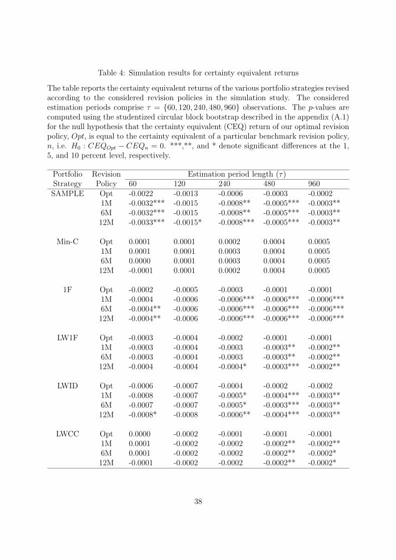
[INSERT TABLE 4 HERE]

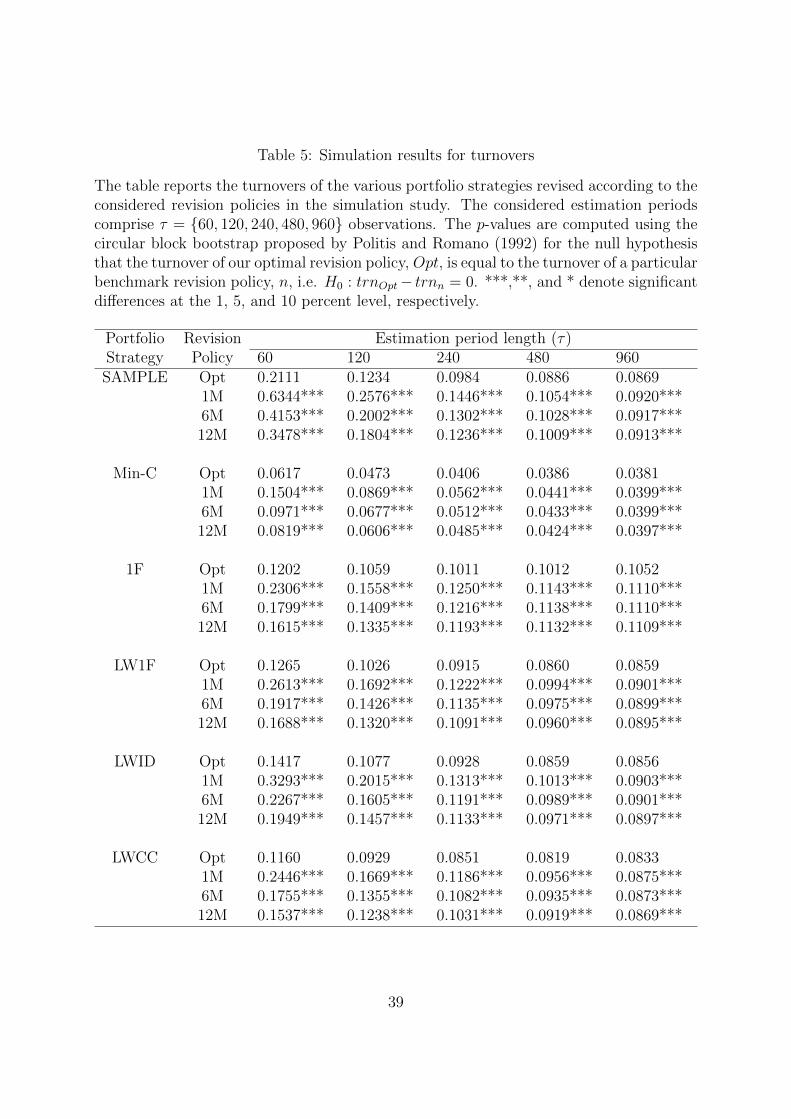
The average monthly turnovers of the various portfolio strategies are reported in

Table 5. The results demonstrate that our proposed revision policy yields a dramatic

decrease in turnover compared to the considered benchmark revision frequencies. The

observed turnover reductions are statistically significant for all portfolio strategies and

estimation period sizes. In particular, we observe for the estimation period comprising

60 months a decrease in turnover between 48% (1F) and 66% (SAMPLE) vis-a-vis the

commonly applied monthly revision frequency. Compared to the six and twelve months

revision frequencies, we find similar figures, though the reductions become unsurprisingly

smaller due to the lower turnover of these benchmarks. Specifically, we observe that the

turnover of the portfolios revised according to our policy is reduced between 33% (1F and

LWCC) and 49% (SAMPLE) compared to a six months revision frequency. For revision

frequencies of twelve months, we observe reductions between 24% (LWCC and Min-C)

and 39%. The extension of the estimation period from 60 to 120 months is accompanied

by a decrease in the turnover reduction. Correspondingly, we find that our revision policy

reduces the turnover between 32% (1F) and 52% (SAMPLE) compared to the monthly

revision frequency; between 24% (1F) and 38% (SAMPLE) compared to the six month

revision frequency; and between 20% (1F) and 31% (SAMPLE) compared to the twelve

months revision. We ascribe the lower turnover reduction of our revision policy in com-

parison to the results from the shorter estimation period to the generally higher stability

of portfolio weights over time when the estimation period is increased. Accordingly, we

find that the turnover reduction of our revision policy decreases proportionately with the

estimation period length.

19

For the 960 months estimation period, the decrease in turnover attributable to our

revision policy compared to all considered benchmark revision frequencies amounts to

roughly 5% across all portfolio strategies. However, we find that, similar to the out-of-

sample variances, even these small differences are significant.

[INSERT TABLE 5 HERE]

In summary, we find that our portfolio revision policy reduces the out-of-sample

variances as well as the turnover of the considered minimum-variance portfolio strategies

significantly. The observed turnover reductions do not come at the cost of a lower risk-

adjusted performance as measured by the Sharpe ratio or CEQ return. On the contrary,

we even find small increases in the aforementioned performance metrics, especially if the

estimation period is large. In the following, we step away from the clinical conditions

entertained in our simulation study and evaluate our revision policy on real datasets.

4 Empirical Results

4.1 Data

Table 6 provides an overview of the empirical data sets we consider for the empirical

evaluation of our portfolio revision policy. The ten and forty-eight industry portfolios,

as well as the six and twenty-five portfolios sorted by size and book-to-market ratios

represent different cuts of the U.S. stock market and are available from Kenneth French’s

website. The aforementioned data sets span from July 1963 to December 2008.

[INSERT TABLE 6 HERE]

Our single stock data set comprises U.S. single stocks and spans from July 1965 to

December 2008. The construction of the single stock data set is similar to the construc-

tion in Chan et al. (1999), DeMiguel et al. (2009b), and Jagannathan and Ma (2003).

20

Specifically, we select all NYSE, AMEX, and NASDAQ listed stocks from the CRSP data

base that have no missing returns over the entire sample period. From this filtered subset,

we select the 100 largest stocks according to their average market capitalization over the

sample period.

For the risk free rate, we use the 30-day T-bill rate, which we also obtained from

Kenneth French’s website.

4.2 Evaluation of the Optimal Revision Policy

Table 7 presents the out-of-sample variances for the analyzed portfolio strategies revised

according to our optimal portfolio revision policy (Opt), and the benchmark revision

frequencies of one, six, and twelve months. Even though the portfolio variances of the op-

timal revision policy are in general comparable to those with fixed revision frequencies, we

observe several significant deviations for all data sets and portfolio strategies. Regarding

these deviations, two general observations can be made:

First, the larger the asset universes the more significant differences occur. For the

STOCK data set, the SAMPLE and 1F strategies have significantly lower out-of-sample

variances if they are revised according to our revision policy instead of one of the three

fixed revision frequencies. We attribute the significant variance reduction in comparison

to the fixed revision frequencies to a shrinkage-like effect of our revision policy. Unless

alpha takes the value of 1, the revised portfolio weights from our revision policy are

always a weighted average of the new and old portfolio weights (which may themselves

be a combination of less recent weights). The averaging over the new, unbiased portfolio

weights and old, biased13 portfolio weights introduces a bias on the resulting revised

portfolio weights. However, the introduction of the aforementioned bias allows a reduction

in estimation variance and hence a lower mean-squared-error of the revised portfolio

13Even though the old portfolio weights represent unbiased estimates conditional on recent samples, theyrepresent a biased estimate of optimal portfolio weights conditional on the current sample.

21

weights.

[INSERT TABLE 7 HERE]

Second, more significant differences in the out-of-sample variance between our re-

vision policy and the fixed revision frequencies are observed for the extended revision

frequencies, especially for the annual revision frequency. For most data sets and portfolio

strategies, the shorter fixed revision frequencies yield lower portfolio variances compared

to longer frequencies. This observation is not surprising since the shorter the revision

frequency, the faster are the weights adjusted to changing market dynamics, which have

an effect on the optimal weights, e.g. changes in the correlation structure of individual

assets or changes in volatility.

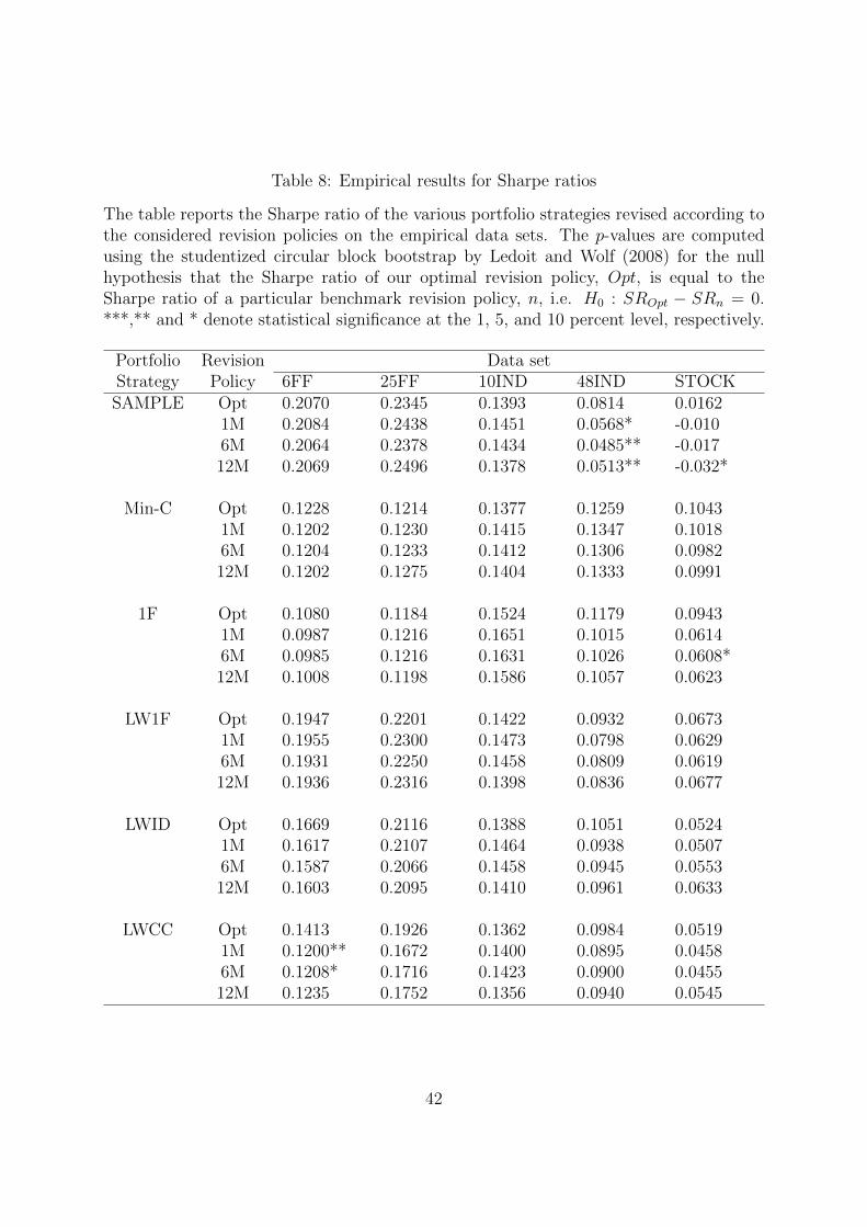
[INSERT TABLE 8 HERE]

The Sharpe ratio and the CEQ return are reported in Tables 8 and 9, respectively.

The CEQ returns are calculated for a risk aversion coefficient of five. We observe only a

few significant performance differences between the optimal revision policy and the fixed

revision frequencies. Specifically, we find significantly higher Sharpe ratios on the 6FF

data set for LWCC, on the 48IND data set for SAMPLE, and on the STOCK data set for

1F and SAMPLE. Except from the observed deviations, we find that the Sharpe ratios

and CEQ returns for the fixed revision frequencies are highly comparable to those of the

optimal revision policy.

[INSERT TABLE 9 HERE]

Finally, Table 10 reports the portfolio turnovers. In almost all cases the turnover of

our optimal revision policy is significantly lower than the turnover of the corresponding

portfolio strategies revised according to a fixed revision frequency. The largest turnover

differences are observed when comparing our revision policy to the monthly revision fre-

quency. In particular, the turnover of SAMPLE is reduced by 71.3% for the STOCK

22

data set, while the turnover of the Min-C strategy is reduced by 77.6% for the 25FF data

set. However, even when compared to the annual revision frequency, we find consider-

able reductions in turnover. For instance, the turnover of the 1F and SAMPLE portfolio

strategies for the STOCK data set is reduced by 36.3% and 41.7%, repectively. The av-

erage reductions according to the portfolio strategies considering all revision frequencies

add up to 36.7% (SAMPLE), 27.7% (1F), 27.3% (LW1F), 23.3% (LWID), 28.0% (LWCC),

and 38.9% (Min-C). These results indicate that the average reductions in turnover are

highly comparable across portfolio strategies, which underpins the robustness of our revi-

sion policy in the sense that the turnover reductions are independent of the choice of the

portfolio strategy.

[INSERT TABLE 10 HERE]

4.3 Optimal Revision Policy in Presence of Transaction Costs

So far we have discussed the results in the absence of transaction costs. However, trans-

action costs play a vital role in the practical implementation of portfolio strategies. Ac-

cordingly, from a practical perspective it is most interesting to look at the performance

of the portfolio strategies after transaction costs. Furthermore, the portfolio performance

evaluation in the presence of transaction costs allows us to evaluate the economic value,

i.e. the increase in portfolio performance attributable to the turnover reduction of our

portfolio revision policy.

Critically, our portfolio revision policy does not take trading costs into account

when determining the optimal fraction of wealth to be kept in the old portfolio weights.

While our portfolio revision policy could easily be modified to take transaction costs

into account by altering the objective function to a maximization of the expected out-

of-sample CEQ return minus trading costs, we find that this does not yield a favorable

out-of-sample performance. We attribute this to the trade-off between an estimation error

prone quantity (the expected out-of-sample performance) and a constant, estimation error

23

free quantity (trading costs).14

In order to assess the performance of our proposed optimal revision policy in the

presence of transaction costs, we report the differences of the Sharpe ratios and CEQ

returns between our optimal revision policy and the fixed revision frequencies for all data

sets and portfolio strategies as a function of transaction costs. Specifically, we apply one

way transaction costs between 0 and 100 bps. We have chosen this interval for one-way

transaction costs because the mid-point of 50 bps results in round-trip transaction costs of

1%. This is in line with recent literature on transaction costs and portfolio optimization.15

Hence, we regard it as a positive result when our optimal revision policy achieves a better

performance compared to fixed revision frequencies with transaction costs of 50 bps or

lower. The lower the transaction costs that are required to outperfrom the fixed revision

frequencies, the better is the performance of our proposed optimal revision policy.

[INSERT FIGURE 1 HERE]

Figure 1 presents the Sharpe ratio differences for the STOCK data set.16 All curves

of the Sharpe ratio differences have a positive slope due to our proposed revision policy

generating consistently lower turnover compared to the fixed revision frequencies. Ac-

cordingly, the performance differences increase with higher transaction costs. In almost

all cases the curve of the Sharpe ratio differences is above the zero line (where the Sharpe

ratio difference is zero). This indicates a higher performance even without transaction

14Our observations are in line with DeMiguel et al. (2010), who consider trading costs directly in theobjective function of a myopic mean-variance portfolio optimization problem.

15See for example DeMiguel et al. (2009b), Kirby and Ostdiek (2011), and Brandt et al. (2009). Allaforementioned papers employ proportional one-way transaction costs of 0.5% over a similar time periodas the one in this paper. Brandt et al. (2009) further model proportional transaction costs in a moresophisticated way by treating them as a function of the market value and time so as to account for thefact that transaction costs are typically lower for stocks with a large market capitalization and thattransaction costs have declined over time. In doing so, they also include the empirical observations ofother authors regarding transaction costs (e.g., Keim and Madhavan (1997) and Hasbrouck (2009)).The average proportional one-way transaction costs of the function are again 0.5%, which furthersupports this number to be an appropriate assumption.

16We present the figures for the Sharpe ratio and CEQ return differences only for the STOCK data set,since it represents tradable capital market data. The figures for the remaining data sets are omitteddue to space considerations, but are available upon request from the authors.

24

costs. This is the case for SAMPLE, Min-C and 1F. For LW1F with a revision frequency

of twelve months the Sharpe ratio differences curve intersects the zero line before trans-

action costs of 10 bps, which means that for transaction costs larger than 10 bps our

revision policy attains a higher Sharpe ratio. For LWID with revision frequencies of one

and six months we observe the intersections at similar low transaction costs. Only for

LWID and LWCC with a revision frequency of twelve months do we find higher Sharpe

ratios for our revision policy at considerably higher transaction costs of above 90 and 50

bps, respectively.

In addition to these strong empirical results, we also note significant Sharpe ratio

differences (at the 10% level) at or below transaction costs of 50 bps for many portfolio

strategies and revision frequencies. Significant results are indicated by the intersection of

the lower confidence band and the zero line. Not surprisingly, we find the strongest results

for the highest revision frequency and portfolio strategies with higher portfolio turnovers.

In these cases we observe a steeper slope of the Sharpe ratio differences curves and the

confidence bands, as well as an intersection of these curves with the zero line at relatively

low transaction costs.

Figure 2 depicts the CEQ return differences for the STOCK data set. Overall, the

results are highly comparable to those for the Sharpe ratio differences. All of the curves

representing CEQ differences have a positive slope. The slope, again, increases with higher

revision frequencies. For SAMPLE, Min-C, 1F, and LW1F, the CEQ return difference

curves always lie above the zero line, resulting in larger CEQ returns for our proposed

revision policy already at zero transaction costs. The highest transaction costs - where

the zero line is intersected - are observed for LWID with a revision frequency of twelve

months. For the remaining three cases (LWID and LWCC) where the CEQ difference is

negative at zero transaction costs the intersections of the CEQ return differences curve

and the zero line are at 40bps or below.

As for the Sharpe ratio differences, the CEQ return differences are in many cases

25

significantly different from zero, with the strongest results achieved for those portfolio

strategies and revision frequencies with the largest turnover, i.e. SAMPLE and 1F.

[INSERT FIGURE 2 HERE]

In addition to the evaluation of statistical significance, we also aim to highlight the

economic significance of our results. Comparing the differences of CEQ returns between

the portfolios revised according to our optimal revision policy and portfolios revised ac-

cording to a fixed revision frequency, we obtain the maximum management fee an investor

would be willing to pay for our revision policy. At transaction costs of 50 bps an investor

would be willing to pay an annual management of 1,716 basis points (SAMPLE), 358 basis

points (1F), 60 basis points (LW1F), 48 basis points (LWID), 44 basis points (LWCC),

and 52 basis points (Min-C). These results show that our proposed revision policy deliv-

ers consistent and economically meaningful performance gains when transaction costs are

applied.

For the remaining data sets (6FF, 25FF, 10Ind, and 30 Ind), we observe a similar

pattern for the Sharpe ratio and CEQ return differences.17 We find a positive slope for

the Sharpe ratio and CEQ return difference curves across all data sets and for all portfolio

strategies. Furthermore, in most cases, our proposed revision policy either has a positive

Sharpe ratio or the CEQ return differences already at transaction costs of zero, or the

difference curves intersect the zero line at reasonable transaction costs of 50 bps or lower.

However, with regard to the statistical significance of performance differences we find

more statistically significant results at transaction costs of 50 bps or below for the data

sets with larger asset universes (25FF, 48IND and STOCK) and find less strong results

for the smaller data sets (6FF and 10IND).

If we consider the economic significance across all data sets and portfolio strategies,

for transaction costs of 50 bps, an investor with a risk aversion of five would be willing

17Due to space considerations, we do not show the results here. However, the results are available fromthe authors upon request.

26

to pay an annual management fee of 101 basis points for the optimal revision strategy

compared to a fixed annual revision frequency. Compared to the semi-annual and monthly

revision frequency, the corresponding management fees amount to 112 and 168 basis

points, respectively. Focusing on the considered portfolio strategies, we find that an

investor would be willing to pay an annual management fee of 435 basis points (SAMPLE),

120 basis points (1F), 53 basis points (LW1F), 48 basis points (LWID), 93 basis points

(LWCC), and 14 basis points (Min-C), respecively. All of the aforementioned numbers

can be considered economically meaningful.

5 Conclusion

In this paper, we developed a novel approach to portfolio revision based on the expected

out-of-sample performance of the underlying portfolio strategy. Contrary to the commonly

applied fixed revision frequencies to portfolio revision, which suggest revision of a portfolio

after a predefined time period, our policy determines if and how much of the previous

portfolio weights need to be revised. Our approach is thereby purely data driven, requiring

no calibration or threshold to trigger the revision of the portfolio. In particular, our

revision policy builds on the Jackknife procedure proposed by Basak et al. (2009) to

estimate the expected out-of-sample moments of portfolios. Based on the estimate of

the expected out-of-sample performance, we derive a closed form solution for the optimal

fraction of wealth to be allocated to the new, in-sample optimal portfolio weights.

Using both simulations and empirical data sets, we demonstrate that our proposed

revision policy leads to a substantial reduction in portfolio turnover compared to all con-

sidered fixed revision frequencies (one, six, and twelve months). Besides a substantially

reduced turnover, the results from our simulation study show that portfolios revised ac-

cording to our revision policy achieve a significantly reduced out-of-sample variance. At

the same time, we find that the risk-adjusted performance, as measured by the Sharpe

27

ratio and CEQ return, is equal to or even slightly above that of the portfolios revised

according to fixed revision frequencies.

Our empirical results confirm the findings from our simulation study to a great

extent. Again, we note that our revision policy yields sizable turnover reductions com-

pared to fixed revision frequencies. In particular, we find that our revision policy reduces

the turnover by up to 77.6% for individual portfolio strategies. On average, we observe

turnover reductions of 44.9%, 27.4%, and 18.9% compared to fixed revision frequencies

of one, six, and twelve months, respectively. At the same time, we find that the out-of-

sample portfolio performance in terms of Sharpe ratios or CEQ returns is similar or even

slightly better than the performance that is obtained by revising portfolios according to

fixed revision frequencies. Accounting for transaction costs, we note that the substantial

turnover reductions attributable to our revision policy translate in many cases into eco-

nomically and statistically significant gains in terms of Sharpe ratios or CEQ returns. On

average, an investor with a risk aversion of five would be willing to pay 101 basis points for

the optimal revision strategy compared to a fixed annual revision frequency. Compared

to the semi-annual and monthly revision frequency, an investor would by willing to pay

112 and 168 basis points, respectively. We observe that the results are especially strong

for data sets with larger asset universes, where the turnover is usually higher.

28

A Appendix

A.1 The studentized circular block bootstrap for hypothesis

testing with the certainty equivalent return

The difference between two Sharpe ratios is given by ∆SR = f(µ1, µ2, σ1, σ2) = µ1σ1− µ2

σ2.

Using uncentered moments as in Ledoit and Wolf (2008), the difference between two

Sharpe ratios may be denoted by ∆SR = f(u) = f(a, b, c, d) = a√c−a2−

b√d−b2 . Equivalently,

the difference between two certainty equivalent returns is given by:

∆CEQ = f(v) = f(a, b, c, d, γ) = a− 1

2γ(c− a2)− b+

1

2γ(d− b2) (29)

where γ denotes the risk aversion coefficient. Let the sample counterpart of ∆CEQ =

f(v) = f(a, b, c, d, γ) be denoted by ∆CEQ = f(v) = f(a, b, c, d, γ). Following equation

(4) of Ledoit and Wolf (2008) the standard error of ∆CEQ is defined as:

s(∆CEQ) =

√∇′f(v)Ψ∇f(v)

T(30)

where ∇′f(v) denotes the gradient of the certainty equivalent difference based on sample

data and Ψ is a consistent estimator of Ψ, which is an unknown symmetric positive semi-

definite matrix. In particular, the gradient of the certainty equivalent return difference is

given by:

∇′f(a, b, c, d, γ) =

(1 + γa,−1− γb,−1

2γ,

1

2γ,

1

2(a2 − c+ d− b2)

)(31)

whereas Ψ is obtained via kernel estimation using the the prewhitened QS kernel of An-

drews and Monahan (1992) as proposed by Ledoit and Wolf (2008). In contrast to the

gradient of the Sharpe ratio difference (see Ledoit and Wolf (2008) p.852), the gradient

of the certainty equivalent difference has five entries since the difference depends not only

29

on the sample moments a, b, c and d but also on the risk aversion coefficient γ.

For the inference concerning the sample certainty equivalent return difference, the stan-

dard error for each bootstrap sample of the proposed studentized circle block bootstrap

by Ledoit and Wolf (2008) is given by:

s(∆∗CEQ) =

√∇′f(v∗)Ψ∗∇f(v)∗

T(32)

where s(∆∗CEQ), f(v∗) and Ψ∗ denote the bootstrap sample counterparts of

s(∆CEQ), f(v) and Ψ. Following Ledoit and Wolf (2008) p.854, we may then de-

fine:

y∗t =(r∗ti − µ∗i , r∗tn − µ∗n, r∗2ti − Γ∗i , r

∗2tn − Γ∗n, 0

)t = 1, .., T (33)

where the last entry in y∗t is zero since the risk aversion coefficient is a constant. Having

the new y∗t and letting l denote the necessary number of blocks to construct a bootstrap

sample, the definitions for ζj and Ψ∗ are those given by Ledoit and Wolf (2008) p.854:

ζj =1√b

b∑t=1

y∗(j−1)b+t t = 1, .., T and Ψ∗ =1

l

l∑j=1

ζjζj′.

30

References

Andrews, D. W. K., and J. C. Monahan (1992): “Heteroskedasticity and Autocor-

relation Consistent Covariance Matrix Estimation,” Econometrica, 59, 817–858.

Arnott, R. D., and J. R. M. Lovell (1993): “Rebalancing: Why, When, How

Often?,” Journal of Investing, 2, 5–10.

Basak, G. K., R. Jagannathan, and T. Ma (2009): “Jackknife Estimator for Track-

ing Error Variance of Optimal Portfolios,” Management Science, 55, 990–1002.

Best, M. J., and R. R. Grauer (1991): “On the Sensitivity of Mean-Variance-Efficient

Portfolios to Changes in Asset Means: Some Analytical and Computational Results,”

Review of Financial Studies, 4, 315–342.

Black, F., and R. Litterman (1992): “Global Portfolio Optimization,” Financial

Analysts Journal, 48, 28–43.

Brandt, M. W., P. Santa-Clara, and R. Valkanov (2009): “Parametric Portfolio

Policies: Exploiting Characteristics in the Cross-Section of Equity Returns,” Review of

Financial Studies, 22, 3411–3447.

Chan, L. K. C., J. Karceski, and J. Lakonishok (1999): “On Portfolio Opti-

mization: Forecasting Covariances and Choosing the Risk Model,” Review of Financial

Studies, 12, 937–974.

Chen, A. H. Y., F. C. Chen, and S. Zionts (1971): “The Optimal Portfolio Revision

Policy,” Journal of Financial and Quantitative Analysis, 44, 51–61.

Chopra, V. K. (1993): “Improving Optimization,” Journal of Investing, 8, 51–59.

Chopra, V. K., C. R. Hensel, and A. L. Turner (1993): “Massaging Mean-

Variance Inputs: Returns from Alternative Global Investment Strategies in the 1980s,”

Management Science, 39, 845–855.

Chopra, V. K., and W. T. Ziemba (1993): “The Effects of Errors in Means, Variances,

and Covariances on Optimal Portfolio Choice,” Journal of Portfolio Management, 4,

6–11.

DeMiguel, V., L. Garlappi, F. J. Nogales, and R. Uppal (2009a): “A Gener-

alized Approach to Portfolio Optimization: Improving Performance by Constraining

Portfolio Norms,” Management Science, 55, 798–812.

31

DeMiguel, V., L. Garlappi, and R. Uppal (2009b): “Optimal Versus Naive Diver-

sification: How Inefficient is the 1/N Portfolio Strategy?,” Review of Financial Studies,

22, 1915–1953.

DeMiguel, V., F. J. Nogales, and R. Uppal (2010): “Stock Return Serial Depen-

dence and Out-of-Sample Portfolio Performance,” Working Paper.

Donhue, C., and K. Yip (2003): “Optimal Portfolio Rebalancing with Transaction

Costs,” Journal of Portfolio Management, 29, 49–63.

Fama, E. F., and K. R. French (1993): “Common Risk Factors in the Returns on

Stock and Bonds,” Journal of Financial Economics, 33, 3–56.

Golosnoy, V., and Y. Okhrin (2009): “EWMA Control Charts for Monitoring Opti-

mal Portfolio Weights,” Sequential Analysis, 26, 195–224.

Green, R., and B. Hollifield (1992): “When Will Mean-Variance Efficient Portfolios

Be Well Diversified,” Journal of Finance, 47, 1785–1809.

Hasbrouck, J. (2009): “Trading Costs and Returns for US Equities: Estimating Effec-

tive Costs from Daily Data,” Journal of Finance, 64, 1445–1477.

Jagannathan, R., and T. Ma (2003): “Risk Reduction in Large Portfolios: Why

Imposing the Wrong Constraints Helps,” Journal of Finance, 58, 1651–1684.

Jobson, J. D., and B. Korkie (1981): “Putting Markowitz Theory to Work,” Journal

of Portfolio Management, 7, 70–74.

Kamin, J. H. (1975): “Optimal Portfolio Revision with a Proportional Transaction

Cost,” Management Science, 21, 1263–1271.

Kan, R., and G. Zhou (2007): “Optimal Portfolio Choice with Parameter Uncertainty,”

Journal of Financial and Quantitative Analysis, 42, 621–656.

Keim, D. B., and A. Madhavan (1997): “Transactions Costs and Investment Style:

An Inter-Exchange Analysis of Institutional Equity Trades,” Journal of Financial Eco-

nomics, 46, 265–92.

Kirby, C., and B. Ostdiek (2011): “It is All in the Timing: Simple Active Portfolio

Strategies that Outperform Naive Diversification,” Journal of Financial and Quantita-

tive Analysis, forthcoming.

32

Kritzman, M., S. Myrgren, and S. Page (2009): “Optimal Rebalancing: A Scalable

Solution,” Journal of Investment Management, 7, 9–19.

Ledoit, O., and M. Wolf (2003): “Improved Estimation of the Covariance Matrix

of Stock Returns with an Application to Portfolio Selection,” Journal of Empirical

Finance, 10, 603–621.

(2004a): “A Well-Conditioned Estimator for Large-Dimensional Covariance Ma-

trices,” Journal of Multivariate Analysis, 88, 365–411.

(2004b): “Honey, I Shrunk the Sample Covariance Matrix,” Journal of Portfolio

Management, 30, 110–119.

(2008): “Robust Performance Hypothesis Testing with the Sharpe Ratio,” Jour-

nal of Empirical Finance, 15, 850–859.

(2011): “Robust Performance Hypothesis Testing with the Variance,” Wilmott

Magazine, forthcoming.

Leland, H. E. (1999): “Optimal Portfolio Management with Transaction Costs and

Capital Gains Taxes.,” Working Paper.

Markowitz, H. (1952): “Portfolio Selection,” Journal of Finance, 7, 77–91.

Markowitz, H., and E. L. van Dijk (2003): “Single-Period Mean: Variance Analysis

in a Changing World,” Financial Analysts Journal, 59, 30–44.

Plaxco, L. M., and R. D. Arnott (2002): “Rebalancing a Global Policy Benchmark,”

Journal of Portfolio Management, 28, 9–22.

Politis, D. N., and J. P. Romano (1992): “A Circular Block-Resampling Procedure

for Stationary Data,” in Exploring the Limits of Bootstrap, ed. by R. LePage, and

L. Billard, pp. 263–270. John Wiley, New York.

Schreiner, J. (1980): “Portfolio Revision: A Turnover-Constrained Approach,” Finan-

cial Management, 9, 67–75.

Sharpe, W. F. (1967): “Portfolio Analysis,” Journal of Financial and Quantitative

Analysis, 2, 76–84.

Siegel, A. F., and A. Woodgate (2007): “Performance of Portfolios Optimized with

Estimation Error,” Management Science, 53, 1005–1015.

33

Tokat, Y., and N. Wicas (2007): “Portfolio Rebalancing in Theory and Practice,”

Journal of Investing, 16, 52–59.

Tu, J., and G. Zhou (2011): “Markowitz Meets Talmud: A Combination of Sophisti-

cated and Naive Diversification Strategies,” Journal of Financial Economics, 99, 204–

215.

34

Table 1: List of considered portfolio strategies

The table lists the minimum-variance portfolio strategies we use to evaluate our portfoliorevision policy.

# Description Abbreviation

1 Minimum-variance portfolio based on the sample covariance matrix SAMPLE

2 Minimum-variance portfolio based on the sample covariance matrixwith short-sale constraints

Min-C

3 Minimum-variance portfolio based on covariance matrix implied bythe single-index model

1F

4 Minimum-variance portfolio as a weighted average of the samplecovariance matrix and the covariance matrix implied by the single-index model

LW1F

5 Minimum-variance portfolio as a weighted average of the samplecovariance matrix and a scalar multiple of the identity matrix

LWID

6 Minimum-variance portfolio as a weighted average between the sam-ple covariance matrix and the covariance matrix implied by theconstant correlation model

LWCC

35

Table 2: Simulation results for variances

The table reports the variances of the various portfolio strategies revised according to theconsidered revision policies in the simulation study. The considered estimation periodscomprise τ = {60, 120, 240, 480, 960} observations. The p-values are computed using thestudentized circular block bootstrap by Ledoit and Wolf (2011) for the null hypothesisthat the variance of our optimal revision policy, Opt, is equal to the variance of a particularbenchmark revision policy, n, i.e. H0 : σ2

Opt − σ2n = 0. ***,**, and * denote significant

differences at the 1, 5, and 10 percent level, respectively.

Portfolio Revision Estimation period length (τ)Strategy Policy 60 120 240 480 960SAMPLE Opt 0.00267 0.00212 0.00194 0.00185 0.00182

1M 0.00310*** 0.00226*** 0.00200*** 0.00189*** 0.00183***6M 0.00311*** 0.00226*** 0.00200*** 0.00189*** 0.00183***12M 0.00312*** 0.00226*** 0.00200*** 0.00189*** 0.00183***

Min-C Opt 0.00219 0.00209 0.00202 0.00198 0.001961M 0.00224*** 0.00211*** 0.00203*** 0.00199*** 0.00196**6M 0.00224*** 0.00211*** 0.00203*** 0.00199*** 0.00196**12M 0.00224*** 0.00211*** 0.00203*** 0.00199*** 0.00196**

1F Opt 0.00215 0.00209 0.00207 0.00204 0.002071M 0.00223*** 0.00218*** 0.00216*** 0.00215*** 0.00213***6M 0.00224*** 0.00218*** 0.00216*** 0.00215*** 0.00213***12M 0.00224*** 0.00218*** 0.00216*** 0.00215*** 0.00213***

LW1F Opt 0.00214 0.00201 0.00192 0.00184 0.001821M 0.00220*** 0.00206*** 0.00195*** 0.00188*** 0.00183***6M 0.00221*** 0.00206*** 0.00195*** 0.00188*** 0.00183***12M 0.00221*** 0.00206*** 0.00195*** 0.00188*** 0.00183***

LWID Opt 0.00227 0.00205 0.00193 0.00185 0.001821M 0.00237*** 0.00213*** 0.00197*** 0.00189*** 0.00183***6M 0.00237*** 0.00213*** 0.00197*** 0.00189*** 0.00183***12M 0.00238*** 0.00213*** 0.00197*** 0.00189*** 0.00183***

LWCC Opt 0.00225 0.00205 0.00194 0.00185 0.001821M 0.00232*** 0.00212*** 0.00198*** 0.00189*** 0.00183***6M 0.00232*** 0.00212*** 0.00197*** 0.00189*** 0.00183***12M 0.00232*** 0.00212*** 0.00197*** 0.00189*** 0.00183***

36

Table 3: Simulation results for Sharpe ratios

The table reports the Sharpe ratios of the various portfolio strategies revised according tothe considered revision policies in the simulation study. The considered estimation periodscomprise τ = {60, 120, 240, 480, 960} observations. The p-values are computed using thestudentized circular block bootstrap by Ledoit and Wolf (2008) for the null hypothesisthat the Sharpe ratio of our optimal revision policy, Opt, is equal to the Sharpe ratio of aparticular benchmark revision policy, n, i.e. H0 : SROpt−SRn = 0. ***,**, and * denotesignificant differences at the 1, 5, and 10 percent level, respectively.

Portfolio Revision Estimation period length (τ)Strategy Policy 60 120 240 480 960SAMPLE Opt 0.0854 0.0865 0.0951 0.0999 0.1002

1M 0.0800 0.0869 0.0922 0.0964** 0.0984*6M 0.0807 0.0867 0.0921 0.0968** 0.0985*12M 0.0791 0.0863 0.0918* 0.0965** 0.0985*

Min-C Opt 0.1190 0.1163 0.1186 0.1219 0.12281M 0.1210 0.1187 0.1197 0.1210 0.12226M 0.1199 0.1183 0.1195 0.1212 0.122212M 0.1182 0.1178 0.1193 0.1209 0.1222

1F Opt 0.1109 0.1032 0.1066 0.1092 0.11001M 0.1095 0.1038 0.1022** 0.1019*** 0.1010***6M 0.1090 0.1032 0.1020** 0.1021*** 0.1010***12M 0.1087 0.1029 0.1015*** 0.1018*** 0.1010***

LW1F Opt 0.1091 0.1015 0.1030 0.1035 0.10241M 0.1097 0.1035 0.1019 0.1012* 0.1008*6M 0.1094 0.1030 0.1017 0.1016 0.100912M 0.1086 0.1026 0.1011 0.1013* 0.1009

LWID Opt 0.1057 0.0975 0.0998 0.1020 0.10141M 0.1051 0.0985 0.0981 0.0991** 0.0996*6M 0.1055 0.0983 0.0980 0.0995* 0.0998*12M 0.1039 0.0979 0.0975 0.0992* 0.0998

LWCC Opt 0.1181 0.1089 0.1065 0.1056 0.10361M 0.1220 0.1108 0.1061 0.1037 0.10216M 0.1219 0.1102 0.1059 0.1040 0.102212M 0.1204 0.1095 0.1055 0.1037 0.1023

37

Table 4: Simulation results for certainty equivalent returns

The table reports the certainty equivalent returns of the various portfolio strategies revisedaccording to the considered revision policies in the simulation study. The consideredestimation periods comprise τ = {60, 120, 240, 480, 960} observations. The p-values arecomputed using the studentized circular block bootstrap described in the appendix (A.1)for the null hypothesis that the certainty equivalent (CEQ) return of our optimal revisionpolicy, Opt, is equal to the certainty equivalent of a particular benchmark revision policy,n, i.e. H0 : CEQOpt − CEQn = 0. ***,**, and * denote significant differences at the 1,5, and 10 percent level, respectively.

Portfolio Revision Estimation period length (τ)Strategy Policy 60 120 240 480 960SAMPLE Opt -0.0022 -0.0013 -0.0006 -0.0003 -0.0002

1M -0.0032*** -0.0015 -0.0008** -0.0005*** -0.0003**6M -0.0032*** -0.0015 -0.0008** -0.0005*** -0.0003**12M -0.0033*** -0.0015* -0.0008*** -0.0005*** -0.0003**

Min-C Opt 0.0001 0.0001 0.0002 0.0004 0.00051M 0.0001 0.0001 0.0003 0.0004 0.00056M 0.0000 0.0001 0.0003 0.0004 0.000512M -0.0001 0.0001 0.0002 0.0004 0.0005

1F Opt -0.0002 -0.0005 -0.0003 -0.0001 -0.00011M -0.0004 -0.0006 -0.0006*** -0.0006*** -0.0006***6M -0.0004** -0.0006 -0.0006*** -0.0006*** -0.0006***12M -0.0004** -0.0006 -0.0006*** -0.0006*** -0.0006***

LW1F Opt -0.0003 -0.0004 -0.0002 -0.0001 -0.00011M -0.0003 -0.0004 -0.0003 -0.0003** -0.0002**6M -0.0003 -0.0004 -0.0003 -0.0003** -0.0002**12M -0.0004 -0.0004 -0.0004* -0.0003*** -0.0002**

LWID Opt -0.0006 -0.0007 -0.0004 -0.0002 -0.00021M -0.0008 -0.0007 -0.0005* -0.0004*** -0.0003**6M -0.0007 -0.0007 -0.0005* -0.0003*** -0.0003**12M -0.0008* -0.0008 -0.0006** -0.0004*** -0.0003**

LWCC Opt 0.0000 -0.0002 -0.0001 -0.0001 -0.00011M 0.0001 -0.0002 -0.0002 -0.0002** -0.0002**6M 0.0001 -0.0002 -0.0002 -0.0002** -0.0002*12M -0.0001 -0.0002 -0.0002 -0.0002** -0.0002*

38

Table 5: Simulation results for turnovers

The table reports the turnovers of the various portfolio strategies revised according to theconsidered revision policies in the simulation study. The considered estimation periodscomprise τ = {60, 120, 240, 480, 960} observations. The p-values are computed using thecircular block bootstrap proposed by Politis and Romano (1992) for the null hypothesisthat the turnover of our optimal revision policy, Opt, is equal to the turnover of a particularbenchmark revision policy, n, i.e. H0 : trnOpt− trnn = 0. ***,**, and * denote significantdifferences at the 1, 5, and 10 percent level, respectively.

Portfolio Revision Estimation period length (τ)Strategy Policy 60 120 240 480 960SAMPLE Opt 0.2111 0.1234 0.0984 0.0886 0.0869

1M 0.6344*** 0.2576*** 0.1446*** 0.1054*** 0.0920***6M 0.4153*** 0.2002*** 0.1302*** 0.1028*** 0.0917***12M 0.3478*** 0.1804*** 0.1236*** 0.1009*** 0.0913***

Min-C Opt 0.0617 0.0473 0.0406 0.0386 0.03811M 0.1504*** 0.0869*** 0.0562*** 0.0441*** 0.0399***6M 0.0971*** 0.0677*** 0.0512*** 0.0433*** 0.0399***12M 0.0819*** 0.0606*** 0.0485*** 0.0424*** 0.0397***

1F Opt 0.1202 0.1059 0.1011 0.1012 0.10521M 0.2306*** 0.1558*** 0.1250*** 0.1143*** 0.1110***6M 0.1799*** 0.1409*** 0.1216*** 0.1138*** 0.1110***12M 0.1615*** 0.1335*** 0.1193*** 0.1132*** 0.1109***

LW1F Opt 0.1265 0.1026 0.0915 0.0860 0.08591M 0.2613*** 0.1692*** 0.1222*** 0.0994*** 0.0901***6M 0.1917*** 0.1426*** 0.1135*** 0.0975*** 0.0899***12M 0.1688*** 0.1320*** 0.1091*** 0.0960*** 0.0895***

LWID Opt 0.1417 0.1077 0.0928 0.0859 0.08561M 0.3293*** 0.2015*** 0.1313*** 0.1013*** 0.0903***6M 0.2267*** 0.1605*** 0.1191*** 0.0989*** 0.0901***12M 0.1949*** 0.1457*** 0.1133*** 0.0971*** 0.0897***

LWCC Opt 0.1160 0.0929 0.0851 0.0819 0.08331M 0.2446*** 0.1669*** 0.1186*** 0.0956*** 0.0875***6M 0.1755*** 0.1355*** 0.1082*** 0.0935*** 0.0873***12M 0.1537*** 0.1238*** 0.1031*** 0.0919*** 0.0869***

39

Table 6: List of data sets

The table lists the various data sets used for the evaluation of the portfolio performance,their abbreviations, the number of assets that each data set comprises, the time pe-riod over which we use data from each particular data set, and the data sources. Alldata sets comprise monthly data and apply in case of portfolio data the value weight-ing scheme to the respective constituents. The data sets from Kenneth French are takenfrom his website http://mba.tuck.dartmouth.edu/pages/faculty/ken.french/data_library.html and represent different cuts of the U.S. stock market. The STOCK dataset comprises single stocks from the Center for Research in Security Prices (CRSP).

# Data set Abbreviation N Time period Source

1 6 Fama and French portfoliosof firms sorted by size andbook-to-market ratio

6FF 6 07/1963-12/2008 K. French

2 25 Fama and French portfo-lios of firms sorted by size andbook-to-market ratio

25FF 25 07/1963-12/2008 K. French

3 10 industry portfolios repre-senting the U.S. stock market

10IND 10 07/1963-12/2008 K. French

4 48 industry portfolios repre-senting the U.S. stock market

48IND 48 07/1963-12/2008 K. French

5 100 Stocks with the largestaverage market capitalization

STOCK 100 07/1963-12/2008 CRSP

40

Table 7: Empirical results for variances

The table reports the variances of the various portfolio strategies revised according tothe considered revision policies on the empirical data sets. The p-values are computedusing the studentized circular block bootstrap by Ledoit and Wolf (2011) for the nullhypothesis that the variance of our optimal revision policy, Opt, is equal to the varianceof a particular benchmark revision policy, n, i.e. H0 : σ2

Opt− σ2n = 0. ***,** and * denote

statistical significance at the 1, 5, and 10 percent level, respectively.

Portfolio Revision Data setStrategy Policy 6FF 25FF 10IND 48IND STOCKSAMPLE Opt 0.00167 0.00152 0.00138 0.00194 0.00503

1M 0.00162** 0.00149 0.00136 0.00189 0.00679***6M 0.00170 0.00156 0.00138 0.00193 0.00632***12M 0.00174* 0.00157 0.00135 0.00203 0.00675***

Min-C Opt 0.00198 0.00186 0.00138 0.00144 0.001531M 0.00201 0.00185 0.00138 0.00140** 0.001506M 0.00200 0.00187 0.00138 0.00143 0.0015212M 0.00201 0.00188 0.00136 0.00143 0.00156

1F Opt 0.00214 0.00299 0.00144 0.00154 0.001771M 0.00222 0.00315** 0.00142 0.00158 0.00245***6M 0.00233** 0.00336** 0.00144 0.00159 0.00253***12M 0.00243* 0.00351** 0.00142 0.00161 0.00247***

LW1F Opt 0.00169 0.00143 0.00136 0.00145 0.001571M 0.00164** 0.00139 0.00134 0.00138** 0.00149*6M 0.00172 0.00145 0.00135 0.00141 0.0015512M 0.00176* 0.00146* 0.00133** 0.00145 0.00158

LWID Opt 0.00167 0.00136 0.00133 0.00154 0.001661M 0.00163 0.00133 0.00131* 0.00145*** 0.00158*6M 0.00168 0.00139 0.00132 0.00148** 0.0016512M 0.00171 0.00141** 0.00130*** 0.00153 0.00172

LWCC Opt 0.00179 0.00153 0.00136 0.00148 0.001581M 0.00193*** 0.00200*** 0.00133 0.00141** 0.00152*6M 0.00205*** 0.00215*** 0.00136 0.00146 0.0015812M 0.00214** 0.00224*** 0.00135 0.00148 0.00159

41

Table 8: Empirical results for Sharpe ratios

The table reports the Sharpe ratio of the various portfolio strategies revised according tothe considered revision policies on the empirical data sets. The p-values are computedusing the studentized circular block bootstrap by Ledoit and Wolf (2008) for the nullhypothesis that the Sharpe ratio of our optimal revision policy, Opt, is equal to theSharpe ratio of a particular benchmark revision policy, n, i.e. H0 : SROpt − SRn = 0.***,** and * denote statistical significance at the 1, 5, and 10 percent level, respectively.

Portfolio Revision Data setStrategy Policy 6FF 25FF 10IND 48IND STOCKSAMPLE Opt 0.2070 0.2345 0.1393 0.0814 0.0162

1M 0.2084 0.2438 0.1451 0.0568* -0.0106M 0.2064 0.2378 0.1434 0.0485** -0.01712M 0.2069 0.2496 0.1378 0.0513** -0.032*

Min-C Opt 0.1228 0.1214 0.1377 0.1259 0.10431M 0.1202 0.1230 0.1415 0.1347 0.10186M 0.1204 0.1233 0.1412 0.1306 0.098212M 0.1202 0.1275 0.1404 0.1333 0.0991

1F Opt 0.1080 0.1184 0.1524 0.1179 0.09431M 0.0987 0.1216 0.1651 0.1015 0.06146M 0.0985 0.1216 0.1631 0.1026 0.0608*12M 0.1008 0.1198 0.1586 0.1057 0.0623

LW1F Opt 0.1947 0.2201 0.1422 0.0932 0.06731M 0.1955 0.2300 0.1473 0.0798 0.06296M 0.1931 0.2250 0.1458 0.0809 0.061912M 0.1936 0.2316 0.1398 0.0836 0.0677

LWID Opt 0.1669 0.2116 0.1388 0.1051 0.05241M 0.1617 0.2107 0.1464 0.0938 0.05076M 0.1587 0.2066 0.1458 0.0945 0.055312M 0.1603 0.2095 0.1410 0.0961 0.0633

LWCC Opt 0.1413 0.1926 0.1362 0.0984 0.05191M 0.1200** 0.1672 0.1400 0.0895 0.04586M 0.1208* 0.1716 0.1423 0.0900 0.045512M 0.1235 0.1752 0.1356 0.0940 0.0545

42

Table 9: Empirical results for certainty equivalent returns

The table reports the certainty equivalent returns of the various portfolio strategies revisedaccording to the considered revision policies on the empirical data sets. The p-values arecomputed using the studentized circular block bootstrap described in the appendix A.1for the null hypothesis that the certainty equivalent (CEQ) return of our optimal revisionpolicy, Opt, is equal to the certainty equivalent of a particular benchmark revision policy,n, i.e. H0 : CEQOpt − CEQn = 0. ***,**, and * denote significant differences at the 1,5, and 10 percent level, respectively.

Portfolio Revision Data setStrategy Policy 6FF 25FF 10IND 48IND STOCKSAMPLE Opt 0.0042 0.0053 0.0017 -0.0012 -0.0114

1M 0.0043 0.0056 0.0019 -0.0022 -0.0178**6M 0.0042 0.0054 0.0018 -0.0027** -0.0172**12M 0.0042 0.0059 0.0016 -0.0027** -0.0196***

Min-C Opt 0.0005 0.0005 0.0016 0.0011 0.00021M 0.0003 0.0006 0.0018 0.0015 0.00016M 0.0003 0.0006 0.0017 0.0013 0.000012M 0.0003 0.0008 0.0017 0.0014 0.0000

1F Opt -0.0003 -0.0010 0.0021 0.0007 -0.00041M -0.0009 -0.0010 0.0026 0.0001 -0.0030**6M -0.0010 -0.0013 0.0025 0.0001 -0.0032**12M -0.0011 -0.0016 0.0024 0.0002 -0.0030**

LW1F Opt 0.0037 0.0047 0.0018 0.0000 -0.00121M 0.0038 0.0051 0.0020 -0.0004 -0.00126M 0.0037 0.0049 0.0019 -0.0004 -0.001412M 0.0037 0.0052 0.0017 -0.0004 -0.0012

LWID Opt 0.0026 0.0044 0.0017 0.0002 -0.00201M 0.0024 0.0043 0.0020 -0.0001 -0.00196M 0.0023 0.0042 0.0019 -0.0001 -0.001812M 0.0023 0.0043 0.0018 -0.0001 -0.0016

LWCC Opt 0.0015 0.0037 0.0016 -0.0000 -0.00181M 0.0004** 0.0024 0.0017 -0.0001 -0.00206M 0.0003** 0.0025 0.0018 -0.0002 -0.002112M 0.0003 0.0026 0.0016 -0.0001 -0.0018

43

Table 10: Empirical results for turnovers

The table reports the turnover of the various portfolio strategies revised according tothe considered revision policies on the empirical data sets. The p-values are computedusing the circular block bootstrap proposed by Politis and Romano (1992) for the nullhypothesis that the turnover of our optimal revision policy, Opt, is equal to the turnoverof a particular benchmark revision policy, n, i.e. H0 : trnOpt − trnn = 0. ***,**, and *denote significant differences at the 1, 5, and 10 percent level, respectively.

Portfolio Revision Data setStrategy Policy 6FF 25FF 10IND 48IND STOCKSAMPLE Opt 0.1408 0.3539 0.0881 0.3359 0.9925

1M 0.2215*** 0.7868*** 0.1604*** 0.8066*** 3.4585***6M 0.1828*** 0.5518*** 0.1207*** 0.5389*** 2.0778***12M 0.1715*** 0.4764*** 0.1023** 0.4624*** 1.7010***

Min-C Opt 0.0143 0.0226 0.0283 0.0434 0.06411M 0.0290** 0.1007*** 0.0773*** 0.1172*** 0.1598***6M 0.0206*** 0.0416*** 0.0397*** 0.0558*** 0.0892***12M 0.0201** 0.0334*** 0.0365*** 0.0472 0.0755*

1F Opt 0.0844 0.1470 0.0680 0.1352 0.11581M 0.1218*** 0.2379*** 0.0997*** 0.1874*** 0.1730***6M 0.1168*** 0.2328*** 0.0885*** 0.1733*** 0.1624***12M 0.1155*** 0.2309*** 0.0821*** 0.1655*** 0.1539***

LW1F Opt 0.1262 0.2850 0.0834 0.1968 0.21741M 0.1990*** 0.5600*** 0.1416*** 0.3643*** 0.3615***6M 0.1638*** 0.4115*** 0.1096*** 0.2694*** 0.2781***12M 0.1535*** 0.3613*** 0.0934* 0.2391*** 0.2504**

LWID Opt 0.0689 0.1985 0.0670 0.2133 0.26401M 0.0899*** 0.3138*** 0.1097*** 0.3957*** 0.4857***6M 0.0804** 0.2430*** 0.0869*** 0.2848*** 0.3586***12M 0.0757 0.2178 0.0744 0.2517** 0.3203***

LWCC Opt 0.0635 0.1618 0.0627 0.1851 0.18851M 0.1067*** 0.2895*** 0.1005*** 0.3292*** 0.2872***6M 0.0969*** 0.2483*** 0.0815*** 0.2461*** 0.2313***12M 0.0925*** 0.2313*** 0.0701 0.2184** 0.2105*

44

Figure 1: Sharpe ratio differences for the STOCK data set

The eighteen panels in this figure show the Sharpe ratio differences (∆ SR) between our proposed revision

policy and fixed revision frequencies of one, six, and twelve months as a function of proportional one-way

transaction costs in basis points (bps). The Sharpe ratio differences are represented by dashed lines while

dotted lines represent the 90% confidence interval. For the confidence interval, we use bootstrapped

standard errors, which we obtain from the studentized circular block bootstrap from Ledoit and Wolf

(2008).

0 20 40 60 80 100

0

0.1

0.2

0.3

SAMPLE (Revision: 1 month)

Proportional trading costs in bps

∆ S

R

0 20 40 60 80 100

0

0.1

0.2

0.3

SAMPLE (Revision: 6 months)

Proportional trading costs in bps

∆ S

R

0 20 40 60 80 100

0

0.1

0.2

0.3

SAMPLE (Revision: 12 months)

Proportional trading costs in bps

∆ S

R

0 20 40 60 80 100

0

0.02

0.04

Min-C (Revision: 1 month)

Proportional trading costs in bps

∆ S

R

0 20 40 60 80 100

0

0.02

0.04

Min-C (Revision: 6 months)

Proportional trading costs in bps

∆ S

R

0 20 40 60 80 100

0

0.02

0.04

Min-C (Revision: 12 months)

Proportional trading costs in bps

∆ S

R

0 20 40 60 80 100

0

0.02

0.04

0.06

0.08

1F (Revision: 1 month)

Proportional trading costs in bps

∆ S

R

0 20 40 60 80 100

0

0.02

0.04

0.06

0.08

1F (Revision: 6 months)

Proportional trading costs in bps

∆ S

R

0 20 40 60 80 100

0

0.02

0.04

0.06

0.08

1F (Revision: 12 months)

Proportional trading costs in bps

∆ S

R

0 20 40 60 80 100

-0.02

0

0.02

0.04

0.06

LW1F (Revision: 1 month)

Proportional trading costs in bps

∆ S

R

0 20 40 60 80 100

-0.02

0

0.02

0.04

0.06

LW1F (Revision: 6 months)

Proportional trading costs in bps

∆ S

R

0 20 40 60 80 100

-0.02

0

0.02

0.04

0.06

LW1F (Revision: 12 months)

Proportional trading costs in bps

∆ S

R

0 20 40 60 80 100

-0.02

0

0.02

0.04

0.06

0.08

LWID (Revision: 1 month)

Proportional trading costs in bps

∆ S

R

0 20 40 60 80 100

-0.02

0

0.02

0.04

0.06

0.08

LWID (Revision: 6 months)

Proportional trading costs in bps

∆ S

R

0 20 40 60 80 100

-0.02

0

0.02

0.04

0.06

0.08

LWID (Revision: 12 months)

Proportional trading costs in bps

∆ S

R

0 20 40 60 80 100

-0.02

0

0.02

0.04

LWCC (Revision: 1 month)

Proportional trading costs in bps

∆ S

R

0 20 40 60 80 100

-0.02

0

0.02

0.04

LWCC (Revision: 6 months)

Proportional trading costs in bps

∆ S

R

0 20 40 60 80 100

-0.02

0

0.02

0.04

LWCC (Revision: 12 months)

Proportional trading costs in bps

∆ S

R

45

Figure 2: Certainty equivalent return differences for the STOCK data set

The eighteen panels in this figure show the Sharpe ratio differences (∆ SR) between our proposed revision

policy and fixed revision frequencies of one, six, and twelve months as a function of proportional one-way

transaction costs in basis points (bps). The Sharpe ratio differences are represented by dashed lines while

dotted lines represent the 90% confidence interval. For the confidence interval, we use bootstrapped

standard errors, which we obtain from the studentized circular block bootstrap described in the appendix

(A.1).

0 20 40 60 80 100

0

0.01

0.02

0.03

0.04

SAMPLE (Revision: 1 month)

Proportional trading costs in bps

∆ C

EQ

0 20 40 60 80 100

0

0.01

0.02

0.03

0.04

SAMPLE (Revision: 6 months)

Proportional trading costs in bps

∆ C

EQ

0 20 40 60 80 100

0

0.01

0.02

0.03

0.04

SAMPLE (Revision: 12 months)

Proportional trading costs in bps

∆ C

EQ

0 20 40 60 80 100

-5

0

5

10

15

x 10-4

Min-C (Revision: 1 month)

Proportional trading costs in bps

∆ C

EQ

0 20 40 60 80 100

-5

0

5

10

15

x 10-4

Min-C (Revision: 6 months)

Proportional trading costs in bps

∆ C

EQ

0 20 40 60 80 100

-5

0

5

10

15

x 10-4

Min-C (Revision: 12 months)

Proportional trading costs in bps

∆ C

EQ

0 20 40 60 80 100

1

2

3

4

5

x 10-3

1F (Revision: 1 month)

Proportional trading costs in bps

∆ C

EQ

0 20 40 60 80 100

1

2

3

4

5

x 10-3

1F (Revision: 6 months)

Proportional trading costs in bps

∆ C

EQ

0 20 40 60 80 100

1

2

3

4

5

x 10-3

1F (Revision: 12 months)

Proportional trading costs in bps

∆ C

EQ

0 20 40 60 80 100

0

10

20

x 10-4

LW1F (Revision: 1 month)

Proportional trading costs in bps

∆ C

EQ

0 20 40 60 80 100

0

10

20

x 10-4

LW1F (Revision: 6 months)

Proportional trading costs in bps

∆ C

EQ

0 20 40 60 80 100

0

10

20

x 10-4

LW1F (Revision: 12 months)

Proportional trading costs in bps

∆ C

EQ

0 20 40 60 80 100

-1

0

1

2

3

x 10-3

LWID (Revision: 1 month)

Proportional trading costs in bps

∆ C

EQ

0 20 40 60 80 100

-1

0

1

2

3

x 10-3

LWID (Revision: 6 months)

Proportional trading costs in bps

∆ C

EQ

0 20 40 60 80 100

-1

0

1

2

3

x 10-3

LWID (Revision: 12 months)

Proportional trading costs in bps

∆ C

EQ

0 20 40 60 80 100

-5

0

5

10

15

x 10-4

LWCC (Revision: 1 month)

Proportional trading costs in bps

∆ C

EQ

0 20 40 60 80 100

-5

0

5

10

15

x 10-4

LWCC (Revision: 6 months)

Proportional trading costs in bps

∆ C

EQ

0 20 40 60 80 100

-5

0

5

10

15

x 10-4

LWCC (Revision: 12 months)

Proportional trading costs in bps

∆ C

EQ

46