A joint International Livestock - CGSpace · PDF file · 2017-04-24Average annual...

Front Cover

Making science work for the poor

�www.cgiar.org/ilri

INTERNATIONAL

ILRILIVESTOCK RESEARCH I N S T I T U T E

PO Box 30709�Nairobi, Kenya�

�PO Box 5689�Addis Ababa�

Ethiopia

Valuing alternative land-use options �in the Kitengela wildlife dispersal area of Kenya��A joint International Livestock Research Institute (ILRI) and African Conservation Centre (ACC) report undertaken for the Kitengela community. �

P. Kristjanson M. Radeny D. Nkedianye R. Kruska R. ReidH. Gichohi F. AtienoR. Sanford�

��

ILRI Impact Assessment Series �No. 10�

September 2002��

�Valuing alternative land-use options in the Kitengela w

ildlife dispersal area of Kenya ILRI Im

pact Assessm

ent Series No.10 Septem

ber 2002��

�

�

Book Mark Ear Back Cover

dispersal area of Kenya

Valuing alternative land-use options �� in the Kitengela wildlife �

� �

ILRIInternational Livestock Research Institute

Valuing alternative � land-use options in the

Kitengela wildlife dispersal �area of Kenya�

�A joint International Livestock Research Institute (ILRI)

and African Conservation Centre (ACC) report undertaken for the Kitengela community. �

P. Kristjanson M. Radeny

D. Nkedianye R. Kruska

R. ReidH. GichohiF. Atieno

R. Sanford��

A joint International Livestock Research Institute (ILRI) and African Conservation Centre (ACC) report undertaken for the Kitengela community.

Valuing Alternative Land-Use Options in the Kitengela Wildlife Dispersal of Kenya

Valuing alternative land-use options in theKitengela wildlife dispersal area of Kenya

A joint International Livestock Research Institute (ILRI) and the African

Conservation Centre (ACC) report undertaken for the Kitengela community.

ILRI Impact Assessment Series 10

September 2002

P. Kristjanson

M. Radeny

D. Nkedianye

R. Kruska

R. Reid

H. Gichohi

F. Atieno

R. Sanford

International Livestock Research Institute

P.O. Box 30709, Nairobi, Kenya

ILRI Impact Assessment Series

©2002 ILRI (International Livestock Research Institute)All rights reserved. Parts of this publication may be reproduced for non-commercial useprovided that such reproduction shall be subject to acknowledgment of ILRI as holder ofcopyright.

ISBN 92-9146-129-6

Correct citation: Kristjanson P., Radeny M., Nkedianye D., Kruska R., Reid R., GichohiH., Atieno F. and Sanford R. 2002. Valuing alternative land-use options in the Kitengelawildlife dispersal area of Kenya. ILRI Impact Assessment Series 10. A joint ILRI(International Livestock Research Institute)/ACC (African Conservation Centre) Report.ILRI, Nairobi, Kenya. 61 pp.

Valuing Alternative Land-Use Options in the Kitengela Wildlife Dispersal of Kenya

Table of Contents

List of Tables iii

List of Figures v

Acknowledgements vi

Abstract 1

1 Introduction 3

1.1 Changing land-use in Kitengela 5

1.2 Livestock and wildlife populations 7

1.3 ACC pastoral survey 8

1.4 Summary of findings from related studies 9

2 Methods 11

3 Results 15

3.1 Household characteristics 15

3.2 Production systems 15

3.3 Livestock production 16

3.3.1 Livestock holdings 16

3.3.2 Annual offtake and acquisition 19

3.3.3 Livestock losses 20

3.3.4 Herd structure 20

3.3.5 Livestock gross annual output 21

3.3.6 Livestock input costs 26

3.3.7 Net livestock income 28

3.3.8 Comparison of livestock returns across sites 30

3.3.9 Productivity of livestock enterprises 30

i

ILRI Impact Assessment Seriesii

3.4 Crop cultivation 31

3.5 Off-farm earnings 33

3.6 Quarrying 35

3.7 Net income summary by cluster 35

4 Spatial distribution of returns 39

5 Feedback from the community and implications 42

5.1 Wildlife–livestock conflicts 42

5.2 Livestock herd size 42

5.3 Livestock output 43

5.4 Livestock input costs 43

5.5 Crops 43

5.6 Off-farm income 44

5.7 Quarrying 44

5.8 Additional issues raised by workshop participants 44

References 46

Appendix 48

Valuing Alternative Land-Use Options in the Kitengela Wildlife Dispersal of Kenya iii

List of Tables

Table 1. Kitengela and Nairobi National Park wild herbivore and livestock population 1990–1997. 8

Table 2. Mean annual percentage loss of cattle and sheep by different causes on the Lolldaiga Hills ranch, Laikipia District: 1971–1993. 10

Table 3. Descriptive statistics of 171 households from original survey and clustering variables. 11

Table 4. Average values for critical variables by cluster. 12

Table 5. Average land and livestock holdings (absolute numbers) per household by cluster. 17

Table 6. Livestock holdings (TLU) by cluster. 17

Table 7. Livestock holdings (TLU) in other areas and group ranches. 18

Table 8. Annual offtake and acquisition of livestock by value, rate and transaction type. 19

Table 9. Livestock losses (% of the total herd/flock size in September 1999). 20

Table 10. Cattle herd structure by cluster, September 2000. 21

Table 11. Average prices of livestock and products (KSh) in the year 2000. 22

Table12. Summary of gross annual livestock output in a good year (KSh). 22

Table 13. Summary of gross annual livestock output in a bad year (KSh). 23

Table 14. Milk sales revenue and consumption value by cluster. 25

Table 15. Mean annual livestock input cost by cluster (KSh). 27

Table 16. Average input cost comparison (KSh/TLU). 28

Table 17. Net livestock income in a good year by cluster (KSh). 29

Table 18. Net livestock income in a bad year by cluster (KSh). 29

ILRI Impact Assessment Seriesiv

Table 19. Annual livestock net income per TLU and per acre. 30

Table 20. Average crop output per household, kgs/year. 31

Table 21. Average annual gross crop revenues (KSh) value by cluster. 32

Table 22. Average annual net crop income by cluster (including labour costs). 32

Table 23. Average annual net crop income by cluster (excluding labour costs). 33

Table 24. Type of off-farm income activity, number of people involved and estimated off-farm income earnings by cluster (KSh). 34

Table 25. Contribution of off-farm income to total household income. 34

Table 26. Annual net household income by cluster. 37

Valuing Alternative Land-Use Options in the Kitengela Wildlife Dispersal of Kenya v

List of Figures

Figure 1. Distribution of households within the study area. 14

Figure 2. Contribution of sales, consumption and other revenues to gross livestock output. 24

Figure 3. Annual milk sales revenue by cluster (KSh). 25

Figure 4. Contribution of livestock, crops and off-farm income to overall household income in a good year. 36

Figure 5. Contribution of livestock, crops and off-farm income to total household income by cluster. 38

Figure 6. Livestock returns and dry season wildlife (five species—zebra, wildebeest, Grant’s gazelle, Thomson’s gazelle and kongoni) density for surveyed households (KSh/acre): Kitengela wildlife dispersal area. 40

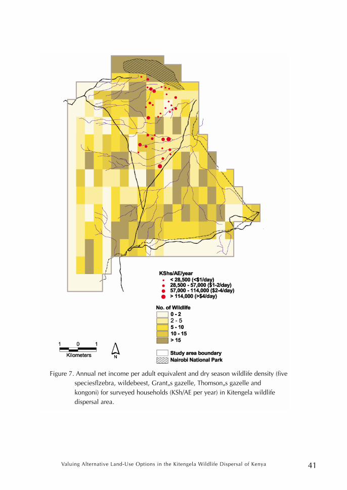
Figure 7. Annual net income per adult equivalent and dry season wildlife density (five species—zebra, wildebeest, Grant’s gazelle, Thomson’s gazelle and kongoni)for surveyed households (KSh/AE/year): Kitengela wildlife dispersal area. 41

ILRI Impact Assessment Seriesvi

Acknowledgements

We are grateful to all organisations and individuals who contributed to this study. Weexpress our gratitude to the 35 households who availed themselves to be interviewed andshared valuable information with the research team during the community workshop.

The enumerators (Benson Patiat, Daniel Isa, Jeremiah Kaloi, Joseph Matanta, SimonMula together with David Nkedienye) worked very hard and were useful resourcepersons throughout the study period. David was an excellent facilitator. He linked theresearch team with the local leaders (chiefs and councillors) and key informants, gatheredbackground information and shared his knowledge and perspectives in interpreting thedata.

We would also like to acknowledge Mario Herrero, Philip Thornton, Mike Rainy,Shauna Burnsilver and Jeff Worden for contributing their expertise and insightfulsuggestions for the implementation of this study and the interpretation of the results.Errors and omissions remain our responsibility, however. Finally, we would like toacknowledge financial support from USAID and ILRI.

Valuing Alternative Land-Use Options in the Kitengela Wildlife Dispersal of Kenya 1

Abstract

East African pastoral and wildlife systems are currently undergoing severe stress dueto a combination of trends including increased human population pressure, economicstructural changes and privatisation of land tenure. These are ecosystems with the richestlarge mammal biodiversity on earth. Most of this wildlife is outside parks in pastoralgrazing areas. Pastoralists in Kenya are facing rapid and widespread changes in theirtraditional lifestyles and appear to be getting poorer. Within the Kitengela wildlifedispersal area adjacent to the renowned Nairobi National Park (NNP), conflicts betweenlandowners and wildlife are becoming more frequent, with serious and potentiallyirreversible implications for both the communities and the wildlife.

This study builds on a previous socio-economic survey undertaken by the AfricanConservation Centre (ACC) in 1999 within the Kitengela wildlife dispersal area.Motivated by requests from community members, the primary objective of this follow-upstudy was to provide critical and timely information to help inform the search for land-use activities that will lead to protection of wildlife corridors and dispersal areas and, atthe same time, maximise returns from the land. The second objective was to exploreways in which to integrate the economic data being supplied by the households withinformation that has been gathered in recent years by ecologists regarding wildlifedistributions and patterns in this area. Since there were few empirical studies upon whichto model this type of integration of economic and ecological data (particularly withinpastoral systems), the approach taken here was fairly novel.

A formal household survey was carried out on a relatively small sample of 35 out ofthe original 171 households interviewed in 1999. Detailed (and sensitive) informationwas sought regarding revenues, costs, income sources and income levels under variousland-use options. The 35 households were then statistically grouped into four clusters,with each cluster made up of relatively homogeneous households with respect to socio-economic and location characteristics. The range of economic activities covered by thesurvey included livestock production, subsistence crop production, quarrying and off-farm income (including wage labour, informal sector employment, remittances fromrelatives and income from investment in businesses).

The results show considerable variation across households’ landholdings, herd size,herd management, level and diversification of income sources and cropping practices.Thus the cluster analysis was useful in terms of distinguishing different types of livelihoodstrategies with respect to both socio-economic characteristics and geographicdeterminants of opportunities (e.g. distance to market).

Income from livestock production was generally low and much lower in years inwhich the long rains failed. Net livestock income averaged around KSh 20,000 per adultequivalent (AE) per year, or roughly US$ (256), per AE per year. On a per acre basis, the

ILRI Impact Assessment Series2

average net income from livestock activities alone was KSh 1400/acre per year, or US$17.95. Milk revenues were important to most households and highly dependent on thetiming and levels of rainfall across all clusters, and surpassed the value of reported milkconsumption.

While 80% of surveyed households grew crops, for most households it is not aprofitable undertaking because when crop output was valued at market prices, the costs ofproduction generally outweighed the potential revenues.

The different types of households (i.e. clusters) varied both in the importance ofalternate income sources and in levels of income. The market-oriented cluster had thehighest levels of annual net income (and highest off-farm income). The traditional clusterhad the lowest annual net income (with 90% of total household income coming fromlivestock). One-third of the respondents had no access to off-farm income, but for theremainder, it can be a very important livelihood option, with some of the ‘wealthiest’households deriving well over half of their income from off-farm sources.

Overall net income per AE levels ranged from KSh 1772–4956/month. This places allof the Kitengela clusters above the rural poverty line (the amount of money considered bythe Government of Kenya to generate inadequate income levels to feed, clothe, educateand pay for basic health care for their families). Two groups fall under the urban povertyline (which is arguably more appropriate for households located so close to Nairobi), andthe third group is barely above it. The market-oriented group, with its smaller averagefamily size, earns roughly twice the income per adult of the established urban poverty line.However, over half of the households (54%) earned less than a dollar a day per adultequivalent, a widely used global measure of poverty. Another 26% earned less than US$ 2per day, 14% earned between US$ 2 and US$ 4 per day and only 2 households (6%)earned over US$ 4 per day per AE.

Looking at the spatial distribution of livestock returns per acre, along with anexamination of the spatial distribution of five species of migratory wildlife during the dryseason, revealed that there are some households earning very little from livestock even inareas with relatively few wildlife. There were also areas with a lot of wildlife wherehouseholds earn high livestock income. These observations do not lend support to thenotion that households in the densest wildlife areas are worse off. There was no easilydiscernible spatial pattern to net incomes per person.

The findings of this study were presented in a workshop with community members andwere well received. Information received from the community was very useful ininterpreting the survey results. Several lessons were also learned regarding methodology,and future analyses will attempt to incorporate more ecological variables in the initialcluster analysis (e.g. measures of soil fertility and degradation, water availability), andaverages from several years of aerial survey data, as well as explore methods of usingremote sensing data.


1 Introduction

Rapidly increasing human population and changing socio-economic lifestyles (leadingto greater natural resource exploitation) have been identified as the greatest threats towildlife conservation within rangelands the world over (WRI 1997; Ellis et al. 1999;Foran and Howden 1999). Within East Africa, changes in land policies, high humanpopulation growth rates, and rapid changes in people’s expectations over the past fewdecades have resulted in the expansion of cultivation, growth in the number ofpermanent settlements, urbanisation and diversification of land-use activities aroundconservation areas. All of these factors have contributed to unprecedentedhuman–wildlife conflicts (Western 1982; Ellis et al. 1999).

The change in land policy from communal to individual landholdings has facilitated amarket-oriented economy, which tends to promote expansion of crop agriculture andcommercialisation of livestock production systems within rangelands (Galaty 1994).Consequences of these changes on land-use patterns include declining ecological,economic and social integrity of rangelands due to fragmentation of landscapes,declining rangeland productivity, diminishing wildlife migratory corridors, wildlifepopulations and diversity, and cultural and economic diversification due to immigration(Gichohi et al. 1996).

In Kenya and many parts of the world, protected areas have proved to be too small tosustainably maintain long-term, viable wildlife populations and diversity (Newmark1993). In Kenya, for example, more than 70% of wildlife is found outside parks andgame reserves on private and communally owned lands within pastoral areas/rangelands(Western and Pearl 1989). In the past, under communal landholdings, wildlife coexistedfreely with people outside the protected areas. Recently, Kenya has experienced rapidchanges in land policies that have transformed former pastoral communal lands intogroup and individual ranches and private holdings. These changes in tenure systems haveled to emergence of a myriad of land-use systems including rain-fed and irrigation cropagriculture, permanent settlement, land sales, quarrying and tented camping sites withinprivate ranches. These changes in land-use are thought to impact negatively on wildlifeconservation and pastoralism as a way of life. Given reduction in land sizes andconnectivity, pastoral mobility and livestock grazing areas have been reduced/curtaileddue to fragmentation, fencing and cultivation. Left with few or no alternatives, pastoralistsare struggling to survive in this harsh environment by diversifying their land-use activities,despite the fact that the conditions are not always suitable for the land-use choices theyare making. Therefore the role of wildlife dispersal areas and migratory corridors outsidethe protected areas is critical to wildlife conservation in Kenya. Given the observed highrate of land sales and fragmentation within the rangelands, viable wildlife corridors needto be established before it is too late.


Wildlife–human conflicts have escalated in recent years in areas adjacent to the parksbecause of changes in land-use, and particularly in response to the expansion andintensification of arable farming, inadequate wildlife control and a ban on hunting. Thesechanges have contributed immensely to the hardships of landowners, who tend to investand lose more money as they try to cope with the wildlife challenges in their land-useenterprises. Despite the changes in socio-economic lifestyles of the pastoralists, fewsystematic, comprehensive and objective studies on the returns to the various land-useoptions (including wildlife) have been done. Past studies mainly focused on the effects ofpastoral land policy changes on livestock productivity (Bekure et al. 1991; Rutten 1992;Homewood 1995). Understanding relative economic returns of different land-use optionsis an important prerequisite to rational and transparent policy formulation and integrationof the present conflicting demands of wildlife habitat, tourism/recreation, livestockgrazing, crop agriculture and other developments within pastoral rangelands (Westernand Gichohi 1993; Ellis et al. 1999). A primary objective of this study is to providecritical and timely information to decision-makers regarding these often conflictingpastoral land-uses.

The study builds on a previous household socio-economic survey undertaken by theAfrican Conservation Centre (ACC) in 1999 within the Kitengela pastoral area adjacent tothe renowned Nairobi National Park (Mwangi and Warinda 1999). With the changes insocio-economic conditions, conflict between landowners and wildlife in this area isincreasingly becoming a major issue. This study aims at informing the search for land-useactivities that will lead to protection of wildlife corridors and dispersal areas and, at thesame time maximise returns from the land. In addressing the challenges that surroundchanges in land-use patterns and economic activities pursued by landowners, the studyattempts to address the following questions:

1. What are the socio-economic characteristics of the families living within the Kitengela wildlife dispersal area?

2. What is the range of economic returns to the different land-use options?

3. What incentives exist or can be introduced to encourage wildlife conservation on private lands?

The study attempts to provide information that will help answer these questions forcommunity members, policy makers and other stakeholders involved in wildlifeconservation. An opportunity-cost approach was taken to estimate economic returns toexisting land-use options and other income-generating activities pursued by Kitengelalandowners. In Kenya, valuing alternative uses of land is viewed as one possibleapproach for estimating the compensation value for wildlife, since wildlife hunting is


illegal and wildlife do not have a recognised market value (other than from tourism)(Norton-Griffiths 1995). The research team used a partial budgeting approach proposedduring a stakeholder workshop held in March 2000. A formal household survey wascarried out on a relatively small sample of households in order to obtain information onrevenues, costs and incomes of the households (comprehensive and sensitiveinformation, hence the small sample). Information on the relative returns of land undervarious uses is expected to contribute towards a more realistic appraisal of the marginalvalue of the land (i.e. the value of one additional acre1 of land) as well as the wildlife thatdepend on it. A second objective of the study was to look at spatial income-distributionpatterns, i.e. do relative economic returns show any discernible spatial patterns and howdo they relate to certain geographic factors such as the distance of the household toNairobi National Park, water sources, the nearest shopping centre, and the closest tarmacroad?

1.1 Changing land-use in Kitengela

Land tenure policies have changed considerably within Kenyan pastoral areas overthe last 40 years. Until the mid-1960’s, land in the pastoral systems was heldcommunally. After Kenya achieved independence from colonial rule, the governmentencouraged private land ownership in pastoral systems, with the aim of intensifying andcommercialising livestock production (Galaty 1994; Homewood 1995). The first majorstep in privatisation was the introduction of the Group Lands Representatives Act in1968, which provided for the adjudication of group ranches (Thompson et al. 2000).Under the Kenya Livestock Development Project (Phase I) funded by the World Bank,each large communally owned piece of Maasai land was adjudicated into several groupranches2 (Grandin 1989). At the same time, some individuals were also able to registertitles over privately owned ranches. Group ranches ranged from 3000 to 151,000 ha,while the individual ranches averaged 800 ha.

Group ranches were seen as a compromise between the Government’s preference forindividual tenure and the production requirements of a semi-arid zone that necessitatesgreater mobility of animals than can be attained under a tenure system that is entirelyprivate. Communal land tenure of large territories and a group ranch approach allowedwildlife to coexist freely with the livestock. However, as a result of inefficiencies andfailures in the operation of the group ranches, the Maasai started pressing for subdivision.The government officially authorised subdivision of ranches in mid-1983. The Kitengela

1 1 acre = 0.4047 hectares.2 Group ranches are organisational structures in which a group of people have a freehold title to land, and aim tocollectively maintain agreed stocking levels and to herd collectively, although livestock are owned and managedindividually.


group ranch, made up of 18,292 ha and 214 registered members, was subdivided in1988. After subdivision of the group ranch, land fragmentation and sales have continuedat a steady and escalating, pace.

Transitions in land tenure have led to changes in land-use activities in the Kitengelaecosystem. This ecosystem acts as a wildlife dispersal area and migratory corridor forNairobi National Park. Maasai pastoralists in this area have diversified into economicactivities other than traditional livestock production. In addition, its close proximity to thecity of Nairobi has attracted non-Maasai and increased the pressure for land forpermanent settlement, industrialisation and speculation. This area is threatened withincreasing human population, permanent settlement and fences, social pressures ontraditional Maasai lifestyles and industrialisation of the Athi-River and Kitengelatownships. These new developments interfere with the seasonal wildlife migratory routesand reduce wildlife ranges and available habitats. These changes in socio-economicconditions and land-use activities appear to be contributing to escalating conflictsbetween landowners and wildlife in the area neighbouring Nairobi National Park.

The Kitengela conservation area covers approximately 390 km2 (GOK 2001b). WhenNairobi National Park was established in 1946 under the National Parks Ordinance of1945, it was immediately recognised that it was too small to meet the ecologicalrequirements for existing migratory wildlife species. Kitengela plains and the Ngong Hillswere thus declared conservation areas. However, the status of Kitengela was neverlegalised and although referred to as a Game Conservation area, the land is nowprivately owned. The Kitengela area therefore presents a great challenge to conservation.The threats arise from several factors, including increasing human population andsettlement along the Mbagathi River (predominantly by the expatriate community whopay high prices to live within view of Nairobi National Park) and the development of theExport Processing Zone (EPZ) in Kitengela town. The EPZ is an industrial park for themanufacture of export goods. Locating the EPZ within this wildlife area has created thefollowing problems:

• Rapid expansion of Athi-River and Kitengela towns into the wildlife habitat as a result of development of subsidiary/ancillary industry and various types of infrastructure supporting the industrial zone.

• Rapid subdivision of land in the neighbourhood—the land is purchased largely by non-Maasai, and in turn the funds are used by the old landowners to fence off the remaining tracts of land, for the purpose of defining individual boundariesor keeping wildlife off the land. Land sales have also provided capital for investment in business in nearby towns and led to settlement expansion.

• Expansion of stone quarrying activities within Kitengela, resulting in conversion of good grazing land into wasteland.


The human population within the Kitengela area has more than doubled in the last 10years, from 6548 in 1989 to 17,347 in 1999 (GOK 1994a; GOK 1994b; GOK 2001a;GOK 2001b). At the same time, the number of households increased nearly five-foldfrom 1989 to 1999 (1044 to 5005 households). The high population growth rateexperienced in this area has been attributed mainly to in-migration, due to Kitengela’sproximity to Nairobi and increasing urban development occurring in the proximity of thetown. The immigrants are mainly from the Kikuyu and Kamba communities.

1.2 Livestock and wildlife populations

Livestock and a large number of wild herbivores dominate the Kitengela ecosystem,with wildebeest and zebra constituting over half the total wildlife population. Otherwildlife species include: Maasai giraffe, Coke’s hartebeest, black rhino, African buffalo,Grant’s gazelle, Thomson’s gazelle, eland, impala and waterbuck and predators such aslions, cheetahs and leopards as well as a high diversity of bird life. The ecosystem formsan important part of the wet season dispersal area for wildlife that lives part of the year inNairobi National Park.

Aerial surveys conducted in the Kitengela dispersal area and Nairobi National Park inJune 1996 and July 1997 revealed that domestic herbivores (i.e. livestock) accounted forup to 80% of the total herbivore population in 1996, and 86% in 1997 (Gichohi andSitati 1997). Nineteen species (5 domestic and 14 wild herbivores) were counted withinan area of 2750 km2 in 1996 and 2925 km2 in 1997 at the beginning of the dry season.Total herbivore (wild and domestic) estimates were 192,862 in 1996 and 272,981 in1997. However, only 11 wild herbivore species were observed in 1996 compared to 14in 1997. The increase in herbivore population of 42% was reported to be statisticallysignificant and resulted in a change in herbivore density, from 70/km2 in 1996 to 90/km2

in 1997. Domestic herbivores accounted for the largest increase of 52%. This could beattributed to a larger sample area in 1997 compared to 1996 and the absence of threewild herbivore species in 1996. The three species (warthog, waterbuck and oryx) occurin small numbers and could have been totally missed during the 1996 survey. The areahas experienced a 50% loss of wildlife populations over the past few years (Table 1).These changes in herbivore populations have been largely attributed to changingconditions resulting from increasing human population and livestock and other humanactivities, as well as climatic changes. Frequent droughts have also occurred in the recentyears especially from 1991 to 1994 and in 1996/1997.

Table 1 also shows that livestock numbers declined markedly in the area untilrecently. Between 1990 and 1996, 45% of all livestock were also lost from the system. Inone year, 1997, livestock populations recovered by more than 50%.


Table 1. Kitengela and Nairobi National Park wild herbivore and livestock population

1990–97.

Year Wild herbivore Livestockpopulation population

1990 73,711 295,660

1992 74,395 237,925

1993 53,771 184,434

1994 38,437 163,954

1996 38,437 154,425

1997 38,693 234,288

Source: Gichohi and Sitati (1997).

1.3 ACC pastoral survey

The objectives of the 1999 ACC pastoral household survey were to examine theimpacts of the wildlife corridor on the welfare of the local community, assess theacceptability of an easement programme to the landowners in the area based on theirwillingness to accept financial compensation in exchange for allowing free movement ofwildlife and examine and propose solutions to the major socio-economic challenges thathave hindered development in the area (Mwangi and Warinda 1999). The survey focusedon the socio-economic factors associated with sustainable livestock production systemsand wildlife conservation in the area and succeeded in describing the range of economicactivities pursued by Kitengela landowners although it did not estimate the returns tothese activities.

The 1999 survey found that landowners in this area suffer frequently from wildlife-related problems. Over 93.5% of the households interviewed reported a very significantincrease in human–wildlife conflicts caused by increased livestock numbers, lack ofeconomic benefits from wildlife, increasing human population, increased risks of humanattack, severe competition for water and grass and frequent predation. Each respondentreported an average loss of KSh 15,903 annually through wildlife-related damages.Livestock predation by wild predators is common during the wet season, with somelivestock killed in the homestead paddocks at night, and others as they graze during theday. Up to 50 attacks were reported, compared to 20 during the dry season. To reducehuman–wildlife conflicts, over 94% of the landowners decided to fence theirhomesteads, 83% their cultivated lands, 16% the grazing lands, while 3% the fallow


land. Over 68% of the respondents reported willingness to leave part of their land(between 0.5–250 acres) unfenced, if in return they were paid a modest sum of moneyfor accommodating wildlife.

The second objective of the 1999 survey, therefore, was to find out what ‘a modestsum of money’ for accommodating wildlife amounted to. Thus it tested a contingentvaluation approach to valuing wildlife by asking respondents how much money theywould be willing to accept in order to compensate for wildlife losses incurred on theirland (i.e. to keep their land open for the use of wildlife as well as their livestock).Unfortunately, the range of responses (i.e. value of compensation) was so large that thismethodology for valuing the land under alternative uses was deemed questionable, andanother approach was sought. The average annual amount of financial compensationdemanded per household/respondent was KSh 60,022 (roughly US$ 920) per acre.

Based (in part) on the findings of the ACC survey, Friends of Nairobi National Park(FONNAP, a non-governmental organisation) initiated a pilot land-leasing project in2000. Landowners were paid KSh 300/acre (approximately US$ 3.80/acre) per year inreturn for agreeing to leave their land open to wildlife and not engage in quarrying,fencing, land subdivision and sale or poaching activities. The pilot project started in April2000 with a total of 214 acres initially signed up under the lease programme. Thisincreased to 2708 acres in January 2001. As of April 2001, there were 8415 acres on thewaiting list. Plans are underway to raise at least US$ 3 million and invest it in anendowment fund where the interest will be used to pay for the leases, consequentlyensuring sustainability of the programme. FONNAP partners include the Wildlife Trustbased in California (USA) and Kenya Wildlife Trust in the UK, Kenya Wildlife Service(KWS), International Fund for Animal Welfare (IFAW)–East Africa, Africa WildlifeFoundation (AWF) and African Conservation Centre (ACC) among others. The leaseprogramme will be strengthened with the purchase of critical pieces/parcels of land. Thisambitious lease programme was officially inaugurated at the launching of the NairobiNational Park Migration Appeal in November 2000.

1.4 Summary of findings from related studies

The problem of human–wildlife conflicts has also been reported in Koiyaki (groupranch), Lemek and Olchoro-Oiroua (individual holdings) in Maasai Mara (Thompson etal. 2000). Apart from competing with the livestock for water and pasture, wildlifefacilitates the transmission of certain livestock diseases, increasing veterinary care costs.Wildlife also increases the cost of maintaining fences around bomas and other structures,indirectly through labour. While predation was cited as a serious problem in these areas,damage caused by disease was much higher. About 5% of livestock deaths were due topredation and approximately 50% due to disease.


In Maasai Mara, revenue-sharing programmes have been initiated through theformation of wildlife associations that include Koiyaki-Lemek and Olchoro OirouaWildlife Trusts. These associations generate income through a game-viewing fee chargedto tourists camping and staying in lodges located on these lands. In addition, there aresmaller associations of landowners that deal with individual or groups of tour operators.These form the main mechanism by which income from tourism is made available togroup ranch members.

The income is paid out as dividends to individual members, or through investment incommunity infrastructure—roads, schools, health facilities and water projects. Thepositive benefits from wildlife in these areas thus have the potential to offset the negativeimpacts of predation. In a privately owned ranch that manages livestock and wildlife inLaikipia district (Mizutani 1998), loss of livestock to carnivores was reported to berelatively small compared to losses from disease (Table 2). The magnitude of loss tocarnivores depended on the type of habitat, policies of livestock management andavailability of natural prey.

Table 2. Mean annual percentage loss of cattle and sheep by different causes on the Lolldaiga Hills

ranch, Laikipia District, 1971–93.

Cause of losses Cattle Sheep

Disease 49.9 59.4Accident 11.9 5.8Theft and missing 14.0 13.4Snake bite 0.9 2.6Carnivores 23.2 18.8

Source: Mizutani (1998).

In Mbirikani and Kimana group ranches near Amboseli National Park, similarhuman–wildlife conflicts were reported (Mbogoh et al. 1999). In these areas, causes ofsuch conflicts included the transmission of diseases from wildlife to livestock, loss oflivestock due to predation and loss of human life. In Mbirikani, income from wildlifetourism did not sufficiently offset the losses incurred by wildlife. In Kimana, apart fromwildlife tourism enterprises, there is a wildlife sanctuary within the ranch that generatesincome directly from tourism. In addition to the wildlife-tourism enterprises, these groupranches receive annual grants of up to KSh one million from Kenya Wildlife Service(KWS), from the gate fee collections of Amboseli National Park as well as employmentopportunities. There is a comprehensive ecological–economic study currently underwayexamining the underlying factors of land-use changes within several group ranches nearAmboseli that takes a similar approach to the one used in this study (Burnsilver 2000).


2 Methods

The first challenge for this study was to limit the number of economic options to beanalysed because the original ACC survey of 171 households demonstrated a wide rangeof resources and income or food generating activities; thus a ‘representative enterprise’approach was sought. This is a partial budgeting approach that is commonly used tocharacterise and analyse crop farm enterprises, but has not been applied widely for semi-pastoral households such as those found in Kitengela (these households are described assemi-pastoral since livestock still move beyond the boundaries of the land that thehousehold owns, but the household is based on a permanent site, usually with somecropping activities).

While a large number of socio-economic factors were examined in the original ACCstudy, 15 variables were chosen as critical factors for a cluster analysis (described below).A brainstorming session with a stakeholder group judged these variables as the mostimportant factors influencing households’ livelihood strategies. The aim of the clusteranalysis was to come up with clusters (groups) of relatively homogeneous households

Selected variables N Mean Median Standard Mini MaxiValid Missing deviation mum mum

Age of respondent (years) 171 0 44 41 14 20 80 Number of dependents 169 2 8 7 5 0 30 Years of formal education 171 0 6 5 6 0 23 Length of stay in the area (years) 168 3 26 25 15 1 74 Amount of land owned (acres) 168 3 156 77 208 2 1,316 No. of cattle sold per year 167 4 4 2 7 0 50 No. of cattle owned (March 1999) 170 1 53 22 87 0 510 Annual milk sales revenue (KSh/year) 160 11 32,076 10,250 58,265 0 491,000 Annual quarrying revenues 170 1 11,635 0 57,407 0 600,000 Land under cultivation (acres) 170 1 2 2 2 0 15 Annual crop income (derived) 171 0 21,010 0 72,835 0 660,000 Kraal distance to the Nairobi National Park (NNP) edge (km) 162 9 7.3 5.9 6.1 0 22.7 Distance to the nearest water point (km) 162 9 1.3 1.2 1.0 0 6.2 Distance to the nearest tarmac road (km) 162 9 6.1 6.6 2.5 0.1 10.3 Distance to the nearest shopping centre (km) 162 9 9.4 9.1 3.1 3.2 16.6

Source: Mwangi and Warinda (1999).

Table 3. Descriptive statistics of 171 households from original survey and clustering variables.


engaged in similar economic activities. The cluster analysis minimises the variationwithin a cluster, and maximises variation between clusters (Solano et al. 2001). A sampleof households from each cluster was then targeted for a detailed survey (using structuredquestionnaires) aimed at calculating the revenues and costs of the livestock, crop andother income-generating options utilised by landowners in each cluster, using a partialbudgeting approach. The 15 factors hypothesised to have a significant influence onhouseholds’ livelihood (or income-generating) opportunities are presented in Table 3.

Details of the statistical procedure used to come up with the household clusters aresimilar to those found in Solano et al. (2001). The steps involved are briefly describedhere. First, an initial factor analysis identified a smaller number of factors explaining themajority of the variation observed among the groups. Out of the 15 variables selected, 8‘factors’ were obtained in this initial step. This was followed by a cluster analysis of the 8factors to identify relatively homogeneous groups of cases based on the 15 selectedvariables. Four principal clusters were identified, with 29, 39, 15 and 46 households. Thetotal number of households captured in these clusters was 129. Table 4 shows the meansof these 15 critical variables by cluster relative to the overall population means (of the171 households surveyed).

Table 4. Average values for critical variables by cluster.

Cluster 1 Cluster 2 Cluster 3 Cluster 4 WeightedTraditional Near Market- Average mean

park oriented

Number of households 29 39 15 46 171 Age of respondent (years) 57 48 39 36 44 Number of dependents 13 7 9 6 8 Years of formal education 2 5 11 5 6 Length of stay in the area (years) 21 36 27 20 26 Amount of land owned (acres) 207 101 85 156 156 No. of cattle sold per year 4 6 2 3 4 No. of cattle owned (March, 1999) 40 55 46 53 53 Annual milk sales revenue (KSh/year) 30,937 43,966 21,934 22,335 32,076 Annual quarrying revenues (KSh/yr) 11,034 13,282 0 5,217 11,635 Land under cultivation (acres) 2 2 6 1 2 Annual crop income (derived) 9,876 14,121 27,867 8,889 21,010 Kraal distance to Nairobi National Park (km) 8.2 3.3 8.7 9.9 7.3 Distance to the nearestwater point (km) 1.3 1.0 0.9 1.7 1.3 Distance to the nearesttarmac road (km) 9.1 11.8 6.7 8.7 6.1 Distance to the nearest shopping centre (km) 7.6 6.4 4.4 6.2 9.4 Gross revenues (milk, quarrying, crops) (KSh/yr) 51,847 71,369 42,790 36,441


Source: Mwangi and Warinda (1999).

The description of the clusters as compared to the whole sample are given below:

• The first cluster includes pastoralists with relatively high landholdings, smaller than average cattle herd size, larger households, relatively low crop income, an older and less educated household head, and was given the description ‘traditional’. This group is located on average 8.2 km far from the park and 9.1 km far from the nearest tarmac road and 7.6 km far from the nearest shopping centre.

• The second cluster was a more diversified group, with relatively large cattle herds, higher revenues from milk sales and some crop and quarrying income. This group of households is located close to Nairobi National Park and has relatively good water point access. The name given to this cluster was ‘near park’.3

• The third cluster was called ‘market-oriented’ since it has more educated household heads, less land but with more of it under cultivation, tends to be closer to a tarmac road and a shopping centre, and is a non-quarrying group.

• The fourth group of households has the lowest gross revenues, is located farthest from the park, has the youngest household head, a smaller household size, average landholdings and cattle herd size, and low crop and milk earnings. Households in this group are quite distant from the nearest tarmac road, water point and shopping centre. It is referred to as the ‘average’ cluster.

Spatial distribution of the households by cluster in relation to the park within thewildlife dispersal area is shown in Figure 1. There are slight differences in climate withinthe dispersal area, with areas near the park receiving slightly more rainfall than areas tothe south of the park.

Given the sensitivity of the questions, length of the survey, and the limited resourcesfor the study, a relatively small sample (35 households) of the original householdsinterviewed was targeted in this follow-up survey. A proportional number of householdswere selected from each cluster: 8 from the traditional cluster, 9 from the near parkcluster, 6 from the market-oriented cluster and 12 from the average cluster. Primary dataon revenues and expenditures for livestock production, crop production, and quarryingactivities was collected from the households in September 2000. Secondary sources of

3 Areas near the park are more prone to wildlife visits on the outward and return migration and the normal dailymovements in and out of the park.


data such as crop prices and historical rainfall patterns were based on interviews withkey informants.

Interviews of the Maasai households were typically based on a single visit to eachhousehold, with follow-up visits for information where the respondents gave conflictinginformation or when a household member who was not available during the first visitneeded to be consulted. Spatial and descriptive analyses of the socio-economic variablesare discussed in the sections that follow. The sample size was too small for meaningfuleconometric analysis.

There were difficulties during the survey arising from the drought that started in 1999and lasted throughout 2000. By September 2000, there were a significant number oflivestock deaths attributed to the drought. This made it difficult for the respondents togive accurate information regarding herd structure, size and breed, since the livestockhad been moved considerable distances from home in search of pasture and water.

Since an objective of the survey was to capture the range of activities and returns tothose activities and not their drought coping strategies, the respondents were asked forinformation regarding a typical good year (defined as both the long and short rainsoccurring) and a typical bad year (defined as the long rains failing).

Figure 1. Distribution of households within the study area.

Source: ILRI (2000), based on 1994 aerial photography (Gichohi 1996).


3 Results

This section discusses the results obtained from the survey regarding householdcharacteristics, production system (livestock and crop production), off-farm income andquarrying activities.

3.1 Household characteristics

Among the Maasai, a household is defined as all those living within the samehomestead, i.e. within the same ‘enkang’ and typically includes the children, husband,wife and also members of the extended family. Out of the 35 respondents, 27 were males(77%) and 8 were females (23%). The household size, expressed in adult equivalents4

(AE), ranged from 1.7 to 27.5 with an overall mean of 6.1 AEs per household. There wereslight variations in household size between clusters with the near park cluster havinglarge households (7.7 AEs) and the market-oriented cluster the smallest (4.2 AEs). Theaverage household size in Kitengela is lower than that reported for Mbirikani (10.8 AEs),but higher than those reported for Kimana (4.1 AEs) (Mbogoh et al. 1999). Therespondents were aged between 20 and 70 years with a mean of 40 years. There were nodiscernible variations in age between the clusters. The level of education (years of formaleducation) among the respondents averaged 6 years and ranged from no formaleducation at all to 20 years of education. About 24% of the respondents had no formaleducation, 47% had less than 10 years of education and 29% had more than 11 years offormal education. The market-oriented cluster had the highest average level of education(11.5 years), while respondents in the traditional cluster had the lowest level of education(4.4 years). Half of the respondents in the traditional cluster had no formal education atall. There was a significant correlation between age of respondent, level of education andhousehold size. The younger respondents were more educated (r = –0.52, p < 0.01), withrelatively smaller household sizes (r = 0.49, p < 0.01).

3.2 Production systems

Pastoralism has historically formed the central element of the Maasai productionsystem living in the Kitengela area adjacent to Nairobi National Park. New employmentopportunities have opened up in recent years in the area with the development of anexport processing zone (EPZ) next to Kitengela town. This, coupled with opportunities topurchase land relatively close to Nairobi, has attracted non-Maasai immigrants toKitengela.

4 The concept of adult equivalent is based on the differences in human nutrition requirements according to age,where: <4, 5–14 and >15 years of age are equivalent to 0.24, 0.65 and 1 adult equivalent, respectively.


Some of the new landowners are interested (and more experienced than the Maasai)in growing crops. Others appear to be land speculators. There is also a small amount ofcommercial production of horticultural products for export occurring but not captured inthis study.

While the local community (Maasai) still focus on livestock production, they havebeen diversifying into cropping (mostly maize, beans and potatoes for subsistence) andselling their land and investing in small businesses, wage labour and quarrying activities.Wage labour appears to be an increasingly important activity, including employment inboth public and private sectors. The range of economic activities covered by the surveyincluded livestock production, subsistence crop production, off-farm income (from wagelabour, remittances from relatives and income from investment in businesses) andquarrying. All 35 households were engaged in livestock production, 28 households (80%)practiced crop production, 21 (60%) received some off-farm income and only 2households (6%) were engaged in quarrying. To obtain more information regardingreturns to quarrying, an additional four households were interviewed solely on theirquarrying activities. While livestock production is still the dominant form of production(all households are involved), subsistence crop cultivation has become a central part oflivelihood strategies, along with off-farm income from wage labour and businessinvestments.

3.3 Livestock production

3.3.1 Livestock holdings

The Maasai keep cattle, sheep and goats (hereafter lumped together as ‘shoats’) andsometimes donkeys for transportation. The average number of cattle owned perhousehold decreased from 71 in 19985 to 58 in September 1999 and 48 in September2000, i.e. a 17% decrease in the drought year. The size of cattle herd per householdranged from 3 to 290. Similarly, the average number of shoats owned per household haddecreased from 152 in 1998 to 88 in September 1999 and to 69 by September 2000, a22% decrease from 1999 to 2000. Herd sizes continued to decrease after September2000 and a halt in livestock deaths due to drought did not come until the end of theyear. Average landholdings and herd sizes by cluster are shown in Table 5.

5 Herd and flock sizes for 1998 were derived from the original ACC survey of 171 households in March 1999.


Table 5. Average land and livestock holdings (absolute numbers) per household by cluster.

Cluster Cattle Sheep GoatsLand Sept. Sept. Sept. Sept. Sept. Sept.(acres) 1999 2000 1999 2000 1999 2000

‘Traditional’ 247 53 42 73 57 27 22 ‘Near park’ 75 41 36 53 38 18 12 ‘Market-oriented’ 119 37 32 44 33 18 13 ‘Average’ 219 85 70 81 66 28 22 ‘All households’ 171 58 48 65 51 23 18

Average landholdings among the clusters ranged from 75–247 acres. Households inthe drier area had approximately 3 times (219 acres) more land than households in thewetter area near the park (75 acres). The average cluster with the second highestlandholding (219 acres) had the largest number of cattle (70) and shoats (88). Sheeprepresented 75% of the shoats while the rest (25%) were goats. The traditional clusterwith the highest landholdings (247 acres) had 42 and 79 head of cattle and shoats,respectively. The average, traditional and near park clusters reported significant decreasesover the year in the number of shoats, i.e. 19, 21 and 30%, respectively.

Livestock holdings were converted to tropical livestock units (TLU), where 1 TLU isequivalent to 250 kg live weight. The TLU enables us to come up with a homogeneousunit for livestock owned for comparison across clusters. In this study, a bull is equivalentto 1.29 TLU, a cow = 1 TLU, a mature steer = 1.05 TLU, a heifer = 0.7 TLU, animmature steer = 0.68 TLU, a calf = 0.4 TLU and a shoat = 0.11 TLU. The TLUs werederived using average weights of the different sex and age categories of cattle and shoatsestimated from previous studies (King et al. 1984; Bekure et al. 1991; KARI/ODA 1996).These are shown in Appendix I.

Table 6. Livestock holdings (TLU) by cluster.

Cluster TLU TLU Decline in TLU/acre TLU/acre TLU/AESept. Sept. herd size Sept. Sept. Sept.1999 2000 % 1999 2000 2000

‘Traditional’ 49.4 41.1 17 0.20 0.17 6.86‘Near park’ 38.7 33.3 14 0.53 0.46 4.83‘Market-oriented’ 35.0 29.6 15 0.31 0.27 6.85‘Average’ 74.5 62.3 16 0.34 0.29 12.58‘Weighted mean’ 52.8 44.4 16 0.31 0.26 8.30


Household herd sizes in September 2000 ranged from 2.4 to 236.7 TLUs. Livestockholdings per acre across the clusters ranged from 0.17 to 0.46 while TLU per adultequivalent across clusters ranged from 4.8 to 12.6 (Table 6). The traditional cluster withthe highest landholdings had the lowest TLU per acre. The TLU per adult equivalent forthis cluster was almost half that of the average cluster. The near park cluster with thesmallest average landholdings and the highest TLU per acre had the lowest TLU per adultequivalent resulting from the relatively large household size (7.7 AEs). The highestTLU/acre thus corresponds to the wettest area of Kitengela wildlife dispersal area. Theaverage cluster with the second largest landholdings had the highest livestock holdingsand TLU per adult equivalent, respectively. The market-oriented cluster had the lowestlivestock holdings (29.6 TLU) and the second highest TLU per acre (0.29). There was asignificant positive correlation between herd size and landholding (r = 0.4, p < 0.01).Similarly, households with more dependents had larger herds (r = 0.6, p < 0.01).

The average livestock holdings, TLU per acre and TLU per adult equivalent across allhouseholds were 44.4, 0.3 and 8.4, respectively (Table 7). The TLU:AE ratio in Kitengelais 50–70% lower than those reported for Talek, Aitong, Lemek, and Nkorinkori locationsin Mara (Thompson et al. 2000).

Table 7. Livestock holdings (TLU) in other areas and group ranches.

Average Average Sample (n) SourceTLU per TLU perhousehold acre

Kitengela 44.4 0.26 35 This study (2001) Olkarkar 150.0 0.24 40 Bekure et al. (1991)Merueshi 130.3 0.10 36 ” Mbirikani 125.6 0.09 250 ”Kimana 28.0 0.37 34 Mbogoh et al. (1999)

Mbirikani 51.0 0.77 27 ”Talek 152.1 25 Thompson et al. (2000)

Aitong 135.6 16 ” Lemek 116.7 21 ” Nkorinkori 99.1 14 ”

However, the average TLU per acre of land in Kitengela is much higher than thosereported for Olkarkar, Merueshi and Mbirikani group ranches in eastern Kajiado in 1982(Bekure et al. 1991). This can be attributed to decreasing/smaller landholdings over time.A similar study (Mbogoh et al. 1999) in Kimana and Mbirikani group ranches withaverage landholdings of 73.8 and 66.6 acres, respectively, reported higher livestockholdings per acre. Although the Kitengela study was conducted in a drought year, the


observed livestock unit per adult equivalent was much higher than those reported forKimana and Mbirikani group ranches in 1999. Since resource endowments and useunder individual land tenure is expected to be different from that in a group ranch andthere are ecological differences between the two areas, the comparisons above should beinterpreted carefully. The average TLU per acre for all households in Kitengela decreasedfrom 0.31 in September 1999 to 0.26 in September 2000. Across all households, averagelivestock holdings decreased from 75 TLUs in 1998 to 52.8 in 1999 and 44.4 in 2000,i.e. a decrease of 41% in the past two years. The declining trend in livestock holdingswas attributed to diseases (especially after the El Niño rains in 1997/98), increasedlivestock sales due to cash demand for household needs, recent droughts (1996/97 and1999/2000), predation, slaughter for home consumption and possible underreporting ofactual numbers of animals by some landowners.

3.3.2 Annual offtake and acquisition

Maasai livestock transactions can be grouped into two major categories: offtake andacquisition. Several methods have been used to compute offtake. Bekure et al. (1991)computed total offtake rate of a herd as sales, exchanges, gifts given out and slaughter.Acquisition was defined as purchases, exchanges and gifts received. Nyariki and Munei(1993) computed offtake rate of a commercial ranch as sales only as a measure of outputdestined for the market. The present study considers sales and slaughter for offtake andpurchases for acquisition. Our approach did not capture exchanges and gifts. Over theSeptember 1999 to September 2000 period each of the 35 households sold, on average,5 cattle and 8 shoats. Table 8 shows reported rates and values for annual offtake andacquisition of livestock per household across the clusters by type of transaction.

Table 8. Annual offtake and acquisition of livestock by value, rate and transaction type.

1. The figures in brackets represent offtake rates for shoats.

Cluster Offtake value and rate Sales and slaughter Acquisition value and rateSales Slaughter as a % of total Purchases Purchases as a %(KSh) (KSh) holdings1 (KSh) of total holdings

‘Traditional’ 46,995 1,830 5.7 (9.4) 9,325 1.4 (1.4)‘Near park’ 37,866 5,378 8.7 (4.4) 10,822 2.7 (0.8)‘Market-oriented’ 80,498 17,642 9.0 (17.6) 17,633 0.8 (7.6)‘Average’ 57,560 1,991 16.2 (18.6 8,217 2.2 (1.8)‘Weighted mean’ 54,013 5,508 9.4 (11.5) 10,754 1.5 (2.6)


Sales represented the most important reason for offtake of livestock. Across allclusters, sales accounted for over 80% of reported offtake value while slaughteraccounted for only 3 to 18% of the offtake value. Annual livestock sales value among theclusters ranged from KSh 37,867 to 80,498. The market-oriented and average clustershad higher livestock sales, with annual sales value of KSh 80,498 and 57,560,respectively. The traditional and near park clusters had lower livestock sales, valued atKSh 46,994 and 37,867 (Table 8). Livestock sales revenue and herd sizes were highlycorrelated (r = 0.6, p < 0.01), i.e. households with large herds sold more livestock. Theaverage annual value of livestock sales per household in Kitengela (KSh 54,013) washigher than that reported for Talek (KSh 33,020), but slightly lower than those reportedfor Lemek (KSh 56,315) in Maasai Mara (Thompson et al. 2000). Offtake rate (as % oftotal livestock holdings) ranged from 5.7 to 16.2% for cattle and 4.4 to 18.6% for shoats.The average and market-oriented clusters had higher offtake rates than did the traditionaland near park clusters for cattle and shoats. Livestock acquisition rates were much lowerthan offtake rates.

3.3.3 Livestock losses

The number of cattle that died from September 1999 to September 2000 accountedfor 15% of the total herd with cluster averages ranging from 10–20% (Table 9). Livestocklosses were significant in the traditional (19.8%) and market-oriented (19.5%) clusters.Seventeen percent of the sheep flock and 22% of the goats died during the period as well(and the fact that so many shoats died is a strong indicator of the seriousness of the 1999drought). Disease and starvation were the major causes of livestock death in the studyarea during this particular year. East coast fever (ECF) was the prevalent disease affectinglivestock, and other diseases mentioned were foot-and-mouth disease (FMD), brucellosisand malignant catarrh fever (MCF).

Table 9. Livestock losses September 1999 to September 2000 (% of the total herd/flock size in

September 1999).

Cluster Cattle Sheep Goats

‘Traditional’ 19.8 21.9 27.4‘Near park’ 10.2 16.6 32.5‘Market-oriented’ 19.5 17.1 22.8‘Average’ 12.8 13.7 12.9‘Weighted mean’ 14.5 16.8 21.8

3.3.4 Herd structure

The structure of cattle herds for the 35 Kitengela households surveyed was classifiedby age and sex. The results are shown in Table 10.


Table 10. Cattle herd structure by cluster, September 2000.

Percent of herdAge and sex ‘Traditional’ ‘Near park’ ‘Market-oriented’ ‘Average’ ‘Weighted of animals mean’

Calves 23 25 20 27 26Steers 17 23 23 19 18 Bulls 3 2 2 3 3Heifers 15 12 12 19 17Cows 42 38 38 33 36

The proportion of the different sexes and age categories ranged from 20–27% forcalves, 17–23% for steers, 2–3% for bulls, 12–19% for heifers and from 33–42% forcows. All herds had a large proportion of females (heifers and cows), ranging from50–57%. The observed herd structure is consistent with those reported for Centraldivision of Kajiado district (Rutten 1992) and Kajiado district as a whole (ASAL 1990).

3.3.5 Livestock gross annual output

Gross annual output of the livestock production system was calculated as theaggregate values of:

• Livestock and by-products sold by the household, including milk, live animals, manure, hides and skin sales.

• Livestock and by-products consumed within the household, including livestock slaughtered and milk consumed.

• Borehole and dip revenues, revenues from traction and revenue from any other livestock or their products (e.g. eggs, chickens).

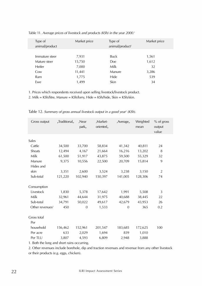
Actual and average market prices were used to value output sales and consumption.The average livestock sales prices and prices of livestock products reported during thesurvey are shown in Table 11.

Mature steers fetched the highest prices in the study area. Prices for immature steerswere slightly higher than for heifers. There were slight price differences across thedifferent categories of shoats. Gross livestock annual output values for a good and a badyear are summarised in Tables 12 and 13.


Table 11. Average prices of livestock and products (KSh) in the year 2000.1

Type of Market price Type of Market priceanimal/product animal/product2

Immature steer 7,931 Buck 1,561 Mature steer 15,750 Doe 1,612 Heifer 7,000 Milk 32 Cow 11,441 Manure 3,286 Ram 1,775 Hide 539 Ewe 1,499 Skin 34

1. Prices which respondents received upon selling livestock/livestock product. 2. Milk = KSh/litre, Manure = KSh/lorry, Hide = KSh/hide, Skin = KSh/skin.

Table 12. Summary of gross annual livestock output in a good year1 (KSh).

Gross output ‘Traditional’ ‘Near ‘Market- ‘Average’ Weighted % of grosspark’ oriented’ mean output

value

SalesCattle 34,500 33,700 58,834 41,342 40,811 24Shoats 12,494 4,167 21,664 16,216 13,202 8Milk 61,500 51,917 43,875 59,500 55,329 32Manure 9,375 10,556 22,500 20,709 15,814 9Hides andskin 3,351 2,600 3,524 3,238 3,150 2Sub-total 121,220 102,940 150,397 141,005 128,306 74

ConsumptionLivestock 1,830 5,378 17,642 1,991 5,508 3Milk 32,961 44,644 31,975 40,688 38,445 22Sub-total 34,791 50,022 49,617 42,679 43,953 26Other revenues2 450 0 1,533 0 365 0.2

Gross totalPerhousehold 156,462 152,961 201,547 183,685 172,625 100Per acre 633 2,029 1,694 839 1,010Per TLU 3,807 4,593 6,809 2,948 3,888

1. Both the long and short rains occurring. 2. Other revenues include borehole, dip and traction revenues and revenue from any other livestock or their products (e.g. eggs, chicken).


Table 13. Summary of gross annual livestock output in a bad year1 (KSh).

Gross output ‘Traditional ‘Near ‘Market’ ‘Average’ Weighted % of grosspark’ oriented’ mean output

value

SalesCattle 34,500 33,700 58,834 41,342 40,811 30 Shoats 12,494 4,167 21,664 16,216 13,202 10 Milk 33,000 36,083 18,375 29,625 30,129 22 Manure 9,375 10,556 22,500 20,709 15,814 12 Hides and skin 3,351 2,600 3,524 3,238 3,150 2 Sub-total 92,720 87,106 124,897 111,130 103,106 76

Consumption Livestock 1,830 5,378 17,642 1,991 5,508 4 Milk 21,745 39,025 14,706 28,313 27,233 20 Sub-total 23,575 44,403 32,348 30,304 32,742 24 Other revenues2 450 0 3,405 0 686 0.5

Gross total Per household 116,746 131,508 160,650 141,435 136,533 100 Per acre 473 1,753 743 1,189 798 Per TLU 2,841 3,949 5,427 2,270 3,075

1. Long rains fail.2. Other revenues include borehole, dip and traction revenues and revenue from any other livestockor their products (e.g. eggs, chicken).

In a good year, about 74% of the gross value of livestock output can be consideredcommercial and 26% for home consumption purposes (Figure 2). Revenues fromborehole, dip, traction and other livestock or their products accounted for less than 1%of total gross output. A major difference between a ‘good year’(defined as both rainsoccurring) and a ‘bad year’(defined as the long rains failing) was reflected in annualrevenues from milk sales and the amount and value of milk consumed. Gross revenuesfrom livestock in a good year (including the value of livestock products consumed) perhousehold ranged from approximately KSh 150,000 to 200,000 (Table 12). Cashrevenues6 ranged from approximately KSh 102,000 to 140,000 and made up 67–78% ofgross livestock output across clusters. Gross livestock output per acre ranged from KSh633 for the traditional cluster to KSh 2029 for the near park cluster.

6 Revenues from sale of livestock and livestock products, excluding value of consumption.


The mean gross livestock output value for the 35 households surveyed was KSh172,625. Gross output per TLU ranged between KSh 2948 and 6809. The market-oriented cluster had the highest gross output value per TLU, which may be due to themuch higher value of cattle sales (and relatively high offtake rates seen in Table 8) for thisgroup of households. Table 13 summarises livestock related revenues in a bad year.

Even in bad years, cash revenues from animal, milk, manure, hides and skin salesmake up roughly 76% of the total value of the livestock enterprise for the Maasaihouseholds. Annual livestock sales revenues in a bad year ranged from KSh 33,700 to58,834 for cattle, and from KSh 4167 to 21,664 for shoats (Table 13). Livestock salesrepresented 32% of gross annual livestock output. The market-oriented cluster had thehighest value of livestock sales of KSh 80,498. Table 13 shows that income from the saleof manure is not insignificant (in some cases it is higher than income from milk sales),with average manure revenues varying between KSh 9375 and 22,500 per cluster. Skinand hides revenue was similar and low across all clusters. Revenues from manure, hidesand skin accounted for approximately 11–14% of the value of gross annual livestockoutput. Revenues from boreholes, traction, dips and other livestock and their productswere negligible.

The value of milk sales in a good year across clusters ranged from KSh 43,875 to61,500, with an overall mean of KSh 55,329 (Table 14). The more traditional pastoralistsearn the most from milk in a good year, but not necessarily in a bad year, when theytypically earn half as much money from milk as they do in a year when both rains occur.In a bad year, households located closer to the park earn about two-thirds as much as in

Good year

Sales74.3%

Consumption25.5%

Otherrevenues

0.2%

Figure 2. Contribution of sales, consumption and other revenues to gross livestock output.

Bad year

Otherrevenues

0.5%Consumption24.0%

Sales75.5%

Good year Bad year


a good year from milk sales, but they still appear to fare better than other members of thecommunity due to higher sales and consumption of milk.

Table 14. Milk sales revenue and consumption value by cluster.

Average gross milk sales: Average gross milk annual revenue (KSh) consumption: annual value (KSh)

Cluster Good year Bad year Good year Bad year

‘Traditional’ 61,500 33,000 32,961 21,745‘Near park’ 51,917 36,083 44,644 39,025‘Market-oriented’ 43,875 18,375 31,975 14,706‘Average’ 59,500 29,625 40,688 28,313‘Weighted mean’ 55,329 30,129 38,445 27,233

Total milk production (sales and consumption) accounted for 54 and 42% of the grossannual livestock output in a good and a bad year. Milk sales alone accounted for 32% ina good year. Average milk production in a good year during the wet (17.5 litres/day) anddry (8 litres/day) seasons was approximately twice as much as production levels in a badyear, with a wet season production of 9.6 litres/day and dry season levels of 4.5litres/day.

The household consumed about 33 and 39% of the total milk produced per day in agood year during the wet and dry seasons, respectively. In a bad year, household milkconsumption increased to 41 and 49% of total output in dry and wet seasons. Theaverage value of milk consumed in a good and a bad year represented about 22 and20% of the total value of gross livestock output. For all households, average milk sales

Figure 3. Annual milk sales revenue by cluster (KSh).

Milk

sal

es r

even

ue


revenue fell from KSh 55,329 in a good year to KSh 30,129 in a bad year (a 46%decrease). Across clusters, the average decline in milk sales revenue ranged from 31% forthe near park cluster to 58% for the market-oriented cluster (Figure 3). Fifty-nine percentof the milk produced is sold, and 41% is retained for household consumption in a goodyear. The value of livestock slaughtered for home consumption was negligible, at 3% ofthe total value of gross annual livestock output. Out of this, shoats accounted for 34% ofthe value of livestock slaughtered for consumption.

3.3.6 Livestock input costs

Livestock input costs include the following:

• veterinary care (vaccines and curative drugs)

• spraying (acaricides), deworming and dipping costs

• hired labour

• mineral supplements

• livestock purchases

• watering and supplement feeds

• operating capital and maintenance costs.

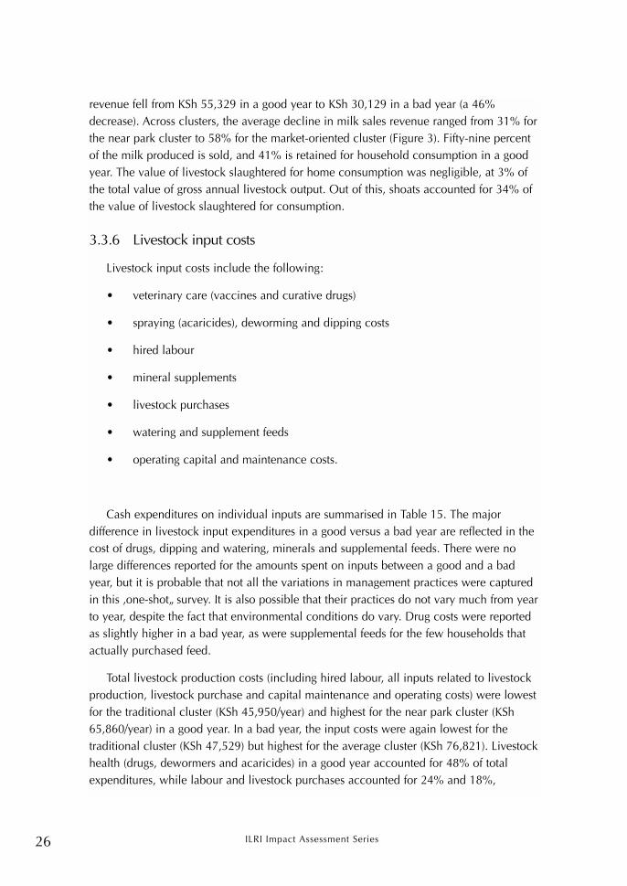
Cash expenditures on individual inputs are summarised in Table 15. The majordifference in livestock input expenditures in a good versus a bad year are reflected in thecost of drugs, dipping and watering, minerals and supplemental feeds. There were nolarge differences reported for the amounts spent on inputs between a good and a badyear, but it is probable that not all the variations in management practices were capturedin this ‘one-shot’ survey. It is also possible that their practices do not vary much from yearto year, despite the fact that environmental conditions do vary. Drug costs were reportedas slightly higher in a bad year, as were supplemental feeds for the few households thatactually purchased feed.

Total livestock production costs (including hired labour, all inputs related to livestockproduction, livestock purchase and capital maintenance and operating costs) were lowestfor the traditional cluster (KSh 45,950/year) and highest for the near park cluster (KSh65,860/year) in a good year. In a bad year, the input costs were again lowest for thetraditional cluster (KSh 47,529) but highest for the average cluster (KSh 76,821). Livestockhealth (drugs, dewormers and acaricides) in a good year accounted for 48% of totalexpenditures, while labour and livestock purchases accounted for 24% and 18%,


respectively. In a bad year, livestock health, labour and purchases accounted for 45, 22and 16% of total expenditures.

For all the households, input costs averaged KSh 59,713 in a good year and KSh65,253 in a bad year (a 9% increase). Average livestock expenditures reported for fourlocations in Maasai Mara (Talek, Aitong, Lemek and Nkorinkori) in 1999 ranged fromKSh 21,735 to 39,630, excluding labour costs (Thompson et al. 2000). Expenditures/TLUon acaricides, drugs, labour and minerals were compared to those reported for Mbirikaniand Kimana group ranches (Mbogoh et al. 1999) in a similar survey carried out inKajiado in 1999 and are presented in Table 16.

Table 15. Mean annual livestock input cost by cluster (KSh).

‘Traditional’ ‘Near park’ ‘Market- ‘Average’ ‘Weightedoriented’ mean’

Good yearDrugs1 7,462 8,861 6,267 7,941 7,758 Dewormers2 7,399 11,144 4,873 10,550 9,010 Acaricides2 11,183 10,848 7,688 15,216 11,880 Mineral supplements 775 633 1,493 3,075 1,650 Supplement feeds 0 0 0 1,133 389 Dipping 0 0 1,500 0 257 Hired Labour2 5,318 23,089 22,000 9,475 14,173 Watering 4,375 0 833 6,392 1,334 Capital 113 463 1,167 475 508 Livestock purchases2 9,325 10,822 17,633 8,217 10,754 Total Expenditure 45,950 65,860 63,454 62,474 59,713 Bad year Drugs1 7,866 9,450 7,725 8,899 8,603 Dewormers2 7,399 11,144 4,873 10,550 9,010 Acaricides2 11,183 10,848 7,688 15,216 11,880 Mineral supplements 700 672 1,190 2,604 1,430 Supplement feeds 0 0 0 11,715 4,017Dipping 0 0 617 0 106 Hired labour2 5,318 23,089 22,000 9,475 14,173 Watering 5,625 0 1,000 9,670 4,773 Capital 113 463 1,167 475 508 Livestock purchases2 9,325 10,822 17,633 8,217 10,754 Total expenditures 47,529 66,488 63,893 76,821 65,254

1. Includes the cost of vaccines and curative drugs. 2. Some input costs (dewormers, acaricides and labour) were recorded for a good year only.


Table 16. Average input cost comparison (KSh/TLU).1

Mbirikani Kimana Kitengela1999 1999 2000

Acaricides 150 170 227Drugs 215 256 1482

Minerals 59 95 32Labour 1773 3273 2714

TLU 51 28 52Sample size 27 34 35

1. Reported livestock numbers were converted to TLU equivalents for comparison. 2. Includes vaccines; 3. Includes the cost of own and borrowed children; 4. Hired labour cost only.Source: Mbogoh et al. (1999).

Input costs in Kitengela (52 TLUs) are perhaps most appropriately compared to thoseof Mbirikani (51 TLUs) since average herd sizes are so similar. Acaricide and labour costsper TLU were lower in Mbirikani, while drug and mineral costs were lower in Kitengela.The differences in acaricide input costs may be explained at least in part by averagelevels of rainfall and ecological differences between the two areas. Kitengela is generallya wetter area than Mbirikani and Kimana, and therefore has a higher population of ticks,thus requiring more acaricides for controlling tick-borne diseases.

3.3.7 Net livestock income

Direct livestock production expenses were deducted from the annual gross outputvalue to derive net livestock income (net income includes value of livestock and productsconsumed by the household valued at market prices). Annual livestock net incomeranged from KSh 87,100 to 138,000, with a mean of KSh 112,916 (Table 17) in a goodyear.


1. Includes value of livestock products consumed by the household.

2. US$ 1 = KSh 78 in November 2000.

In a bad year, levels of net income from livestock decreased significantly, rangingfrom KSh 65,000 to 96,757 (Table 18). The market-oriented cluster had the highest totalnet livestock income, reflecting the higher revenues due to more animal sales. Thiscluster also reported the highest livestock income per adult equivalent, with their smallerhousehold sizes. The cluster nearest the park had the lowest livestock net income, withrelatively high costs coupled with low revenues due to fewer livestock sales, smaller herdsizes and smaller landholdings. The cluster also reported the lowest livestock net incomeper adult equivalent, resulting from a larger household size.

Analysis of variance indicates that there is no significant difference in livestock grossrevenues, input costs and net income across the clusters or across rainfall scenarios (goodversus bad year). This is likely due to the small sample size.

Table 18. Net livestock income in a bad year by cluster (KSh).

Cluster Average Average Net Net Net livestockgross annual gross annual income livestock income perlivestock livestock from income per adult equivalentrevenues production livestock1 adult (US$)2

costs equivalent

‘Traditional’ 116,746 47,529 69,217 11,934 153‘Near park’ 131,508 66,488 65,020 8,444 108‘Market-oriented’ 160,650 63,893 96,757 23,037 295‘Average’ 141,435 76,821 64,614 10,592 136‘Weighted mean’ 136,533 65,254 71,279 11,685 150

1. Includes value of livestock products consumed by the household.2. US$ 1 = KSh 78 in November 2000.

Table 17. Net livestock income in a good year by cluster (KSh).

Cluster Average Average Net Net Net livestockgross annual gross annual income livestock income perlivestock livestock from income per adult equivalentrevenues production livestock1 adult (US$)2

costs equivalent

‘Traditional’ 156,462 45,848 110,613 15,987 205‘Near park’ 152,961 65,861 87,100 11,670 150 ‘Market-oriented’ 201,547 63,454 138,093 34,178 438 ‘Average’ 183,685 62,474 121,212 21,187 272 ‘Weighted mean’ 172,629 59,713 112,916 19,778 254


3.3.8 Comparison of livestock returns across sites

Our estimated range of returns to livestock activities falls within the range estimatedfor several group ranches near Maasai Mara. The Mara study estimated annual net returnsfrom livestock per household ranging from KSh 15,000 to 125,000 (labour costsexcluded) (Thompson et al. 2000). A 1981–83 survey of Olkarkar and Murueshi groupranches in Kajiado District found gross revenues per household ranging from KSh 29,000to 37,000(Bekure et al. 1991). If we inflate these revenues to reflect what that incomewould be worth today, using current cattle prices,7 these figures translate to a range ofKSh 287,100 to 366,300, suggesting that these pastoralists may be earning less than halfthe revenues from livestock than they earned 20 years ago.

3.3.9 Productivity of livestock enterprises

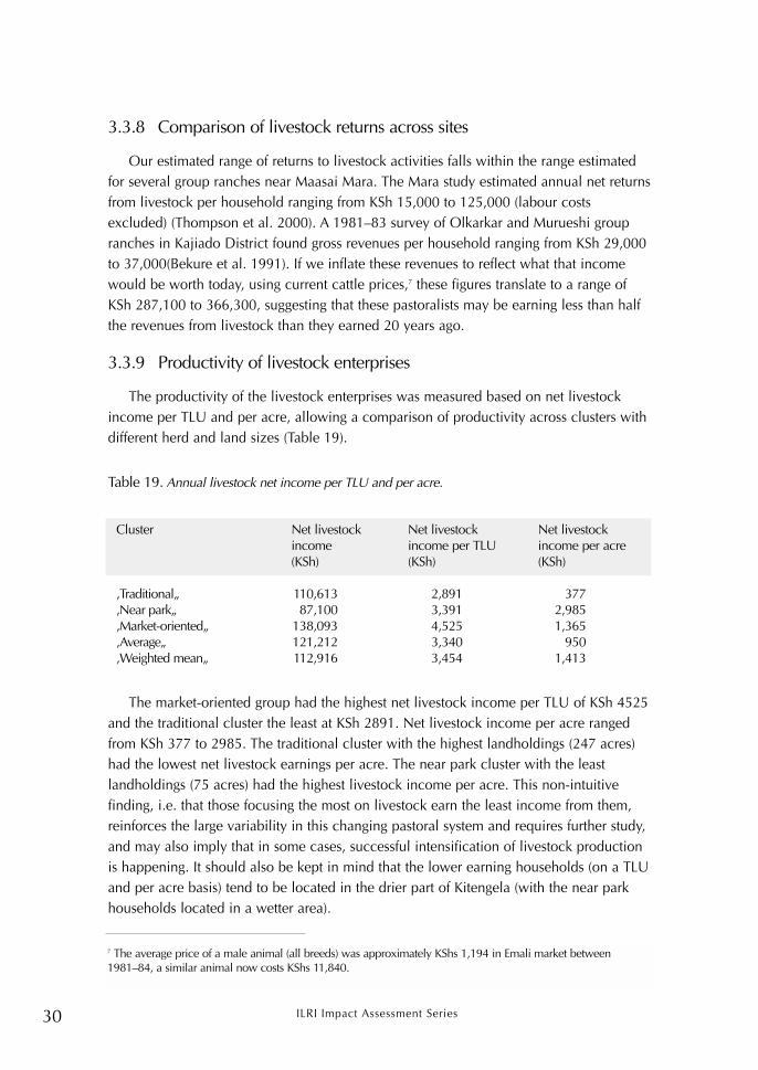
The productivity of the livestock enterprises was measured based on net livestockincome per TLU and per acre, allowing a comparison of productivity across clusters withdifferent herd and land sizes (Table 19).

Table 19. Annual livestock net income per TLU and per acre.

Cluster Net livestock Net livestock Net livestockincome income per TLU income per acre(KSh) (KSh) (KSh)

‘Traditional’ 110,613 2,891 377 ‘Near park’ 87,100 3,391 2,985 ‘Market-oriented’ 138,093 4,525 1,365 ‘Average’ 121,212 3,340 950 ‘Weighted mean’ 112,916 3,454 1,413

The market-oriented group had the highest net livestock income per TLU of KSh 4525and the traditional cluster the least at KSh 2891. Net livestock income per acre rangedfrom KSh 377 to 2985. The traditional cluster with the highest landholdings (247 acres)had the lowest net livestock earnings per acre. The near park cluster with the leastlandholdings (75 acres) had the highest livestock income per acre. This non-intuitivefinding, i.e. that those focusing the most on livestock earn the least income from them,reinforces the large variability in this changing pastoral system and requires further study,and may also imply that in some cases, successful intensification of livestock productionis happening. It should also be kept in mind that the lower earning households (on a TLUand per acre basis) tend to be located in the drier part of Kitengela (with the near parkhouseholds located in a wetter area).

7 The average price of a male animal (all breeds) was approximately KShs 1,194 in Emali market between1981–84, a similar animal now costs KShs 11,840.


3.4 Crop cultivation

Farming is not a major economic activity in Kitengela, although 80% of thehouseholds engaged in some cultivation. Land under crop cultivation was relatively smalland represented less than 2% of the total landholdings. The major crops grown in thisarea were maize, beans, potatoes and sometimes cowpeas, mainly for subsistence.

Table 20 shows the distribution of cropped area among the clusters and average cropproduction levels per household in good and bad years. It can be seen that outputestimates for a bad year still average from 255–852 kgs per household, i.e. even with thefailure of the long rains, most households feel that they get some maize output—one hasto keep in mind that the optimal way of calculating this would be to measure actualhousehold output over several years.

Yields across Kitengela are extremely low. For the traditional cluster, with an averagecropped area of 2.21 acres, maize yields range from roughly 115 to 340 kg/acre. Beanyields range from 316 to 571 kg/acre from a bad year to a good year. Yields appear to bethe highest for the group nearest the park (with an average area under cultivation of 2.38acres). Maize yields vary from around 358 to 605 kg/acre and bean yields from 546 to830 kg/acre.

Table 20. Average crop output per household, kgs/year.

Cluster Maize Beans Cropped % ofBad year Good year Bad year Good year area landholding

(acres) cropped

‘Traditional’ 255 750 698 1,262 2.2 0.8 ‘Near park’ 852 1,440 1,300 1,975 2.4 3.2‘Market-oriented’ 653 1,305 878 1,560 3.9 3.3‘Average’ 446 889 577 1,211 2.4 1.1

For the market-oriented group, with the highest amount of land under cultivation(averaging 3.92 acres), maize yields range from 166–333 kg/acre and bean yields from224–398 kg/acre. For the average cluster (with an average area under cultivation of 2.67acres), maize yields vary from around 167–334 kg/acre and beans from 216–454 kg/acre.It should be noted that the yield variation seen among the clusters likely reflects bothbiophysical differences within the dispersal area (with the wetter areas having highercrop yields than the drier areas) and management differences that are difficult to separateout.


Table 21. Average annual gross crop revenues (KSh) value by cluster.

Cluster Good year revenues1 Bad year revenues2

‘Traditional’ 21,173 17,009

‘Near park’ 33,881 37,992

‘Market-oriented’ 26,033 24,635

‘Average’ 19,423 16,377

1. Good year crop revenues were calculated using the following 1998 localharvest time prices for a 90 kg bag: KSh 600 for maize, KSh 1000 for beans andKSh 500 for potatoes (130 kg bag). Production used for home consumption wasvalued using the same prices.

2. Bad year crop revenues were calculated using the following 1999 local harvesttime prices for a 90 kg bag: KSh 910 for maize, KSh 1800 for beans and KSh 725for potatoes (130 kg bag).

When total crop production was valued using harvest-level prices from‘representative’ good and bad years, the cluster located nearest the park had the highestvalued crop production, followed by the market-oriented cluster, with the average groupearning the least from crops. This ordering holds for both good and bad years. The valueof crop production was actually higher for the near park cluster in a bad year, sincealthough output was lower, prices were significantly higher in the bad year at harvesttime.

The annual crop expenses (labour, seed and ploughing costs) were deducted from thegross output value to derive the net crop income. The net income and crop returns areshown in Table 22.

Table 22. Average annual net crop income by cluster (including labour costs).

Cluster Good year Bad year Good year Bad year(KSh) (KSh) (KSh/acre) (KSh/acre)

‘Traditional’ 1,469 –5,141 668 –2,337‘Near park’ 7,464 12,693 3,110 5,289‘Market-oriented’ –3,295 –2,109 –845 –541‘Average’ 1,215 786 506 327

The cluster located nearest the park, with the least land under crop production(averaging 2.38 acres per household) had the highest net crop income (and income/acre)in a good year, followed by the traditional group (which probably reflects their low inputuse and costs). The market-oriented group (with the most land under crops, at an averageof 3.9 acres per household) earned the least income from crops, except in a bad yearwhen the traditional cluster earned the lowest income and income/acre.


Table 23. Average annual net crop income by cluster (excluding labour costs).

Cluster Good year Bad year Good year Bad year(KSh) (KSh) (KSh/acre) (KSh/acre)

‘Traditional’ 12,290 8,159 5,586 3,709‘Near park’ 18,020 18,607 7,508 7,753‘Market-oriented’ 13,789 14,841 3,536 3,805‘Average’ 11,448 10,683 4,770 4,451

When labour costs are excluded (i.e. family labour time is not valued), the returns tocropping marginally improve in all clusters, ranging from KSh 4770–7508 in a good yearand KSh 3709–7753 in a bad year (Table 23). Similarly, the differences in crop returns ina good and a bad year are smaller (less than KSh 350), except for the traditional cluster.

3.5 Off-farm earnings

Out of the 35 households interviewed, 60% of the respondents had someone in theirhousehold involved in off-farm activities that brought in some income to theirhouseholds. Off-farm income levels were estimated from respondent’s description of thetype of activity and monthly income range (<1000, 1000–5000, 5000–10,000,10,000–20,000, >20,000 KSh/month). Besides the monthly income ranges, therespondents were also asked to estimate the proportion of off-farm income as apercentage of their total household income.

Out of the 24 people with some type of off-farm employment, 11 (46%) engaged invarious business activities, which included selling charcoal or firewood, operating asmall shop, livestock trading, and real estate business. The remaining 13 (54%) wereformally employed in the public and private sectors. The type of off-farm activity andnumber of people involved, and the estimated household monthly and annual off-farmincome levels by cluster are shown in Table 24. Over 80% of those engaged in businessactivities were from the near park and average clusters, while almost half of the formallyemployed were from the average cluster. Approximately 70% of people with some off-farm income were from the near park and average clusters. Respondents near the parkwere more likely to be involved in real estate business.


Table 24. Type of off-farm income activity, number of people involved and estimated off-farmincome earnings by cluster (KSh).1

Type of activity ‘Traditional’ ‘Near park’ ‘Market- ‘Average’oriented’

Government employee – 2 1 3Private sector employee 2 – 2 3 Real estate business – 2 – –Other business 1 3 1 4Average monthly off-farm income (KSh) 938 7,000 9,583 6,250Average annual off-farm income (KSh) 11,250 84,000 115,000 75,000

1. Monthly and annual off-farm income was estimated using midpoints of the income rangesreported by respondents.

The off-farm income levels ranged from KSh 939 per month for the traditional clusterto 10 times higher for the market-oriented group (Table 24). Extrapolating to estimateannual off-farm earnings suggests a substantial contribution to household earnings for 3of the 4 clusters (75,000 to 115,000 KSh/year). This extrapolation needs to be treatedwith caution, however, as it assumes regular monthly payments throughout the year,which may or may not occur, and accurate estimates of non-farm earnings areacknowledged to be very difficult information to obtain.

Respondents were asked to estimate how much of their overall income came from offfarm sources (Table 25). The ratio of off-farm income to total household income8 variedfrom 0 to 90% for all households. One-third of the households received no income fromoff-farm sources, while another one-third received between 10 and 30% of their totalhousehold income from off-farm sources.

Table 25. Contribution of off-farm income to total household income.

Proportion of off-farm Number of As a percentage of allincome to total household respondents households interviewedincome (%)

0 12 3410–30 12 3431–60 5 14>61 6 17Total 35 100

8 Total household income includes net income from livestock and crops in a good year and off-farm income.


For the 35 sampled households, off-farm income accounted for an average of 38% oftotal household income (Figure 4). Among the clusters, off-farm income accounted for 9to 47% of total household income. The near park and market-oriented groups had higherpercentages of total household income attributable to off-farm sources, which equals to47 and 46%, respectively. In the average cluster, where at least 75% of the householdsreceived some off-farm income, off-farm income accounted for 38% of total householdincome. In contrast, the ratio of off-farm to total household income in the traditionalcluster was low, i.e. 9%.

3.6 Quarrying

Out of the 35 households randomly selected from each cluster, only two (6%) wereengaged in quarrying. To obtain more information on returns to quarrying, an additionalfour households engaged in quarrying were interviewed. Annual gross revenues fromquarrying ranged from KSh 98,400 to 880,200. Annual costs (excavation, drilling,blasting, shaping and loading) ranged from KSh 39,740 to 64,200. For those who leasedout land, there were no expenses involved. Net income earned from quarrying variedconsiderably, from KSh 34,200 to 840,460. We were not able to estimate net returns peracre. A number of landowners nearer the Park (especially at Emakoko) decided to filltheir quarries after realising how destructive the activity could be to their land. Most ofthose who own quarries do not engage themselves directly in quarrying, but lease outsmall parts of their land so that they can receive monthly payments from companiesengaged in the excavation activities. The richest area in building stones in Kitengelaremains the Enkurunka valley, which runs along the Kapio tributary (of the EmpakasiRiver). Besides recent demand for building stones from the cement factories nearby (EastAfrican Portland Cement Company and more recently Bamburi Cement), there is also anincreased demand for quarry chips which are used in the manufacture of cement. Weestimate that less than 15 landowners have leased their land to quarry operators in thestone-rich zone (Enkurunka and Emakoko). There is suitable land that has not been putunder quarries and may be susceptible in the future if landowners do not have othersources of income.

3.7 Net income summary by cluster

Net household income is an aggregate value of livestock, crop and off-farm income.Quarrying income is not included here since only two households out of the 35 wereengaged in quarrying. For the 35 households surveyed, total livestock and off-farmincome averaged 61% and 38% of household income (Figure 4).


The traditional cluster had the lowest off-farm income, contributing to the lowestoverall income of KSh 123,332 per year (Table 26). Earnings from agriculture (crops andlivestock) amounted to KSh 112,082, or (US$ 14379 annually, which works out to roughlyUS$ 5.82/acre per year for this group with an average landholding of 247 acres).

The group located nearest to the park earns the least from livestock, but the most fromcrops in a good year, coupled with a fairly high off-farm income. Their total earnings ofKSh 178,564 is equivalent to US$ 2289/year. Average annual income from the farm(crops and livestock) for this cluster works out to KSh 94,564 (US$ 1212, or US$15.54/acre per year) for this group that has the smallest average landholdings (75 acres).Thus in a good year, it is this group that earns the most income on a per acre basis fromfarming and livestock

The market-oriented household cluster earned the most from livestock and off-farmincome, but earned the least from crops, probably because their crop input costs arehigher than the other groups (and they are growing maize in a dry area, where millet orsorghum would be more appropriate). This cluster earned the most overall due to theirhigh off-farm income earnings. Their average total annual earnings of KSh 249,799convert to US$ 3203. The average annual crop and livestock income of KSh 134,799(US$ 1728) works out to KSh 1133/acre (US$ 14.52/acre), for a mean land size of 119acres within this cluster. The cluster named average, distinguished largely by its averagelandholding and herd size characteristics, has low crop revenues, and livestock and off-farm income levels that fall in between the lowest and highest extremes for each group.

61%

1%

38%

Livestock

Crops

Off-farm

Figure 4. Contribution of livestock, crops and off-farm income to overall household income in agood year.

9 US$ 1=KSh 78 in November 2000.


Their average total annual earnings of KSh 197,427 convert to US$ 2531. This group hasan average agricultural earnings of KSh 122,427 (US$ 1570, or US$ 7.17/acre for anaverage landholding of 219 acres).

Table 26. Annual net household income by cluster.

Cluster Good year annual net Average Total Totalhousehold income1 (KSh/year) from: adult annual monthly

Livestock Crops Off-farm Total equivalent income income/(AE) /AE AE

‘Traditional’ 110,613 1,469 11,250 123,332 5.8 21,264 1,772 ‘Near park’ 87,100 7,464 84,000 178,564 7.7 23,190 1,932 ‘Market-oriented’ 138,093 -3,295 115,000 249,799 4.2 59,476 4,956 ‘Average’ 121,212 1,215 75,000 197,427 6.1 32,365 2,697

1. Includes value of livestock and crop products consumed by the household.

Income from livestock accounted for 49–90% of total household income acrossclusters. Household off-farm income ranged from 9–47%, and crop income accountedfor less than 2% of total income with the exception of the near park cluster (4%).Livestock income in the traditional cluster represented 90% of total household income(Figure 5). The near park cluster had similar contributions to household income fromlivestock (49%) and off-farm income (47%). Off-farm income is substantial for all but thetraditional cluster. Despite the considerable variation between clusters in these incomecalculations, an analysis of variance revealed that statistically there were no significantdifferences among the clusters regarding net incomes from livestock, off-farmopportunities and crops. Across all households, there was no statistically significantrelationship between wealth level (measured using herd and land sizes as wealth proxies)and percent contribution of income from livestock to total household income (excludingquarrying). The above results are likely due to the small sample size.

A recent welfare monitoring survey established a rural poverty line for Kenyans of KSh1239/adult equivalent per month, and an urban poverty line of KSh 2648 per month(GOK 2000). Kenyans living below these standards are thus considered to generateinadequate income levels to feed, clothe, educate and pay for basic health care for theirfamilies. All the Kitengela groups are above the rural poverty line and two are under theurban poverty line. One group is barely above the urban poverty line, which is arguablymore appropriate for households located so close to Nairobi. The market-oriented group,with its smaller average family size, earns roughly twice the income per adult equivalentof the established urban poverty line.


Figure 5. Contribution of livestock, crops and off-farm income to total household income by cluster.

Off-farm

Crops

Livestock

Traditional Near park Market oriented Average

Cluster-20%

0%

20%

40%

60%

80%

100%

Per

cent

con

trib

utio

n to

hou

seho

ld in

com

e


10 The information on spatial distribution of migratory wildlife during the dry season included here is not idealsince it comes from a single dry season aerial survey. Work is currently underway to develop both dry and wetseason distribution maps based on 4–5 years of aerial survey data.

4 Spatial distribution of returns

Figure 6 shows livestock returns per acre for the surveyed households, along with thespatial distribution of five species of migratory wildlife (aggregated, including zebra,wildebeest, Grant’s gazelle, Thomson’s gazelle and kongoni) during the dry season.While the sample size was too small to undertake statistical analysis of the explanatorypower of spatial determinants of household income levels, the relative level of returnswas mapped out in order to see if any interesting patterns could be observed.10

Figure 6 shows that 9% of the respondents (3 households) were making greater thanUS$ 40/acre (>3200 KSh), 11% (4 households) were making between US$ 20–40/acre(1600–3200 KSh) and 14% (5 households) were making between US$ 10–20/acre(800–1600 KSh). The other 66% (23 households) made less than US$ 10/acre (800 KSh).Four of the households with higher livestock earnings were near the park, but a few werelocated relatively far from the park.

In relation to where the most wildlife are found during the dry season, it can beobserved that there are some households earning very little from livestock even in areaswith fewer wildlife. There are also areas with a lot of wildlife where households areearning high livestock income, which does not support the notion that households in thedensest wildlife areas are worse off.

When incomes were examined on a per adult equivalent (AE) basis, annual netincome (including livestock, crop, off-farm and quarrying incomes) per adult equivalentranged from KSh 25,762 to 795,300 (Figure 7). Over half of the households (54%) earnedless than a dollar a day per adult equivalent, a widely used global measure of poverty.Another 26% earned less than US$ 2 per day (KSh 28,500–57,000/AE per year), 14%earned between US$ 2 and US$ 4/day (KSh 57,000–114,000/AE per year). Only 2households (6%) earned over US$ 4 per day (>KSh 114,000/AE per year). In over half ofthe households, cropping costs were greater than the value of the output they produce ina good year (excluding family labour costs). There is no easily discernible spatial patternto net incomes per person, with the few higher income households distributedthroughout the study area. Other than the fact that the wealthiest households do not fallin the ‘pixels’ with the most wildlife, a relationship between income and wildlife cannotbe seen using this income measure either.


Figure 6. Livestock returns and dry season wildlife (five species—zebra, wildebeest, Grant’s gazelle, Thomson’s gazelle and kongoni) density for surveyed households (KSh/acre) in Kitengela wildlife dispersal area.

Sources: Survey results and Gichohi (1998), unpublished data.


Figure 7. Annual net income per adult equivalent and dry season wildlife density (fivespecies—zebra, wildebeest, Grant’s gazelle, Thomson’s gazelle and kongoni) for surveyed households (KSh/AE per year) in Kitengela wildlife dispersal area.


5 Feedback from the community andimplications

A workshop with community members, including those involved in the survey plusseveral chiefs and a councillor from the area was held in April 2001 in Kitengela town.The objective of the workshop was to present the survey findings to the community andelicit feedback from them. The major issues that arose and main topics of discussionduring the daylong workshop are summarised below by topic.

5.1 Wildlife–livestock conflicts

Livestock deaths due to predators were major concerns expressed by manycommunity members at this time of the year (beginning of long rains). High presence ofwildlife was reported in the dispersal area, including buffalo, zebra, and eland whichwere roaming outside the park. Wildebeest were also calving in areas around Lenchaniand Enkirgirri. Predation by leopard, lion, cheetah and hyena had increased, with morethan 20 sheep killed the night before the workshop. Residents think the reason conflictshave increased is that wildlife prefers to graze in the areas outside the park wherelivestock graze. Wildlife avoid the park because high grass provides cover for ambushpredators such as lion.

5.2 Livestock herd size

Despite decreasing cattle herds over the years (1998, 1999 and 2000), cattle numbersprobably did not drop as much as indicated by the survey figures. The declining trend incattle numbers was attributed to the following factors:

• Increased cattle sales due to high demand for cash to meet household needs such as school fees, medical care and others

• Increased incidence of disease (East Coast fever, ECF)

• Frequent droughts (1996/97 and 1999/2000) and

• Underestimation of herd sizes due to cultural beliefs

Herd sizes for shoats derived from the survey were said to be consistent with theactual situation. Shoat numbers have drastically decreased over the three years. Outbreakof the blue tongue disease after the long El Niño rains in 1997/98 coupled with droughtand predation from wildlife has contributed to declining shoat numbers.


11 Derived income includes value of output sold and value of output consumed within the household.

5.3 Livestock output

Participants largely agreed with the survey definitions of a good versus a bad year, i.e.good year when both long and short rains fall and bad year when the long rains fail.Among the Maasai, good year scenarios are characterised by good precipitation, plentyof milk and lower incidence of disease. On the other hand, bad years are characterisedby the failure of the long rains (‘Inkokua’), because the long rains generate the mostpasture. Even when the short rains (‘Oltumuret’) come, the year could still be considereda bad one since precipitation is almost always low without the long rains.

Milk and live animal sales profits depend on rainfall. Milk provides income to mosthouseholds in the study area. Participants perceived the value of livestock slaughtered forhome consumption to be very low. After discussions, which included the range of valuesas compared to the average values presented to them, the figures were thought to berepresentative of what happens within the community.

Manure sales were dependent on proximity to either shopping centre or good road(accessibility). The price of manure was higher for those households nearer to the roadsthan those farther away. Average prices as reported by the participants ranged from KSh3500–4000 per lorry carrying 7 t of manure.

5.4 Livestock input costs

Ticks had increased rapidly since the onset of the rains and the cost of acaricides andcurative drugs had also increased. Participants generally agreed with the concept ofderived income11, which includes sales and consumption, given the fact that if you do notproduce for household consumption, you would buy from the market, hence byproducing for consumption, the household saves some money.

5.5 Crops

Crop yield figures from the survey were considered to be very high by manyworkshop participants. A consensus was reached after considerable discussion that ingeneral, maize yields vary from 4–5 bags/acre while bean yields vary from 6–7 bags/acrein a good year, which is lower than the average yields of 9 bags/acre for maize and 13bags/acre for beans from the survey findings. Crop cultivation differs between the Maasaiand the immigrants from other tribes. Among the Maasai, crop cultivation is purely forsubsistence as opposed to their immigrant counterparts. Maasai devote most of their time


to livestock-related activities and very little time is spent on crop production. Lack oftechnical knowledge on crop cultivation among the Maasai has led to:

• Intercropping of more than two crops, e.g. maize, beans, potatoes and bananas leading to low yields,

• Late land preparation, planting and weeding and

• Use of poor quality seeds.

Land preparation costs were considered high, ranging from KSh 1500–4000/acre forcultivated land and new land, respectively.

5.6 Off-farm income

Off-farm income levels, especially for those involved in small businesses, may havebeen negatively affected by the drought. Participants reported that some small shopsmight have closed during the drought due to lack of business.

5.7 Quarrying

The participants agreed that the relatively high returns we presented could beattributed to some landowners who leased land to big cement producing companies.Other landowners sold a lot of hard-core in addition to leasing out land.

5.8 Additional issues raised by participants included:

• Across the community, record keeping is poor for sales or production amounts (for both crops and livestock).

• Drugs and technical assistance are very costly and there are no veterinarians to assist, therefore most people treat livestock themselves.

• Lack of water is a major problem for livestock and crop production.

• The immigrants make more profits from crop cultivation than the Maasai.

• More education was needed for the local people and organisations such as ILRI and ACC could assist through provision of funds to the needy students and development of schools.

• Land sizes are shrinking and therefore intensification is inevitable.

• Wildlife predation, crop damage and spread of diseases were reported to have increased resulting in people–wildlife conflicts. Good fencing around


homesteads and sharing of wildlife revenues with the local community were perceived as possible solutions.

• Commercial livestock production, a gradual change to improved livestock breeds, and education on animal and crop husbandry were seen as ways to increase agricultural productivity in this area.


ReferencesArid and Semi-arid Lands (ASAL). 1990. Kajiado district atlas. Ministry of Reclamation and

Development of semi-arid areas and wastelands, Kajiado, Kenya. 123 pp.Azumi E. and Mia M. 1993. Wildebeests and wheat: Crafting a land policy in Kenya’s Maasailand.

John F. Kennedy School of Government, Harvard University, USA. 55 pp.Bekure S., de Leeuw P.N., Grandin B.E. and Neate P.J.H. (eds). 1991. Maasai herding: Analysis of

the livestock production system of Maasai pastoralists in eastern Kajiado district, Kenya.ILCA Systems Study 4. ILCA (International Livestock Centre for Africa), Addis Ababa,Ethiopia. 172 pp.

Burnsilver S. 2000. Critical factors affecting Maasai pastoralism: The Amboseli region, Kajiadodistrict, Kenya. PhD Proposal, Colorado State University, Fort Collins, Colorado, USA.

Ellis J., Reid R., Thornton P. and Kruska R. 1999. Population growth and land-use change amongpastoral people: Local processes and continental patterns. In: David E. and David F. (eds),

Proceedings of the VIth international rangeland congress, 19–23 July 1999. Townsville,Queensland, Australia. pp. 168–169.

Foran B. and Howden M. 1999. Nine global drivers of rangeland change. In: David E. and David F.

(eds), Proceedings of the VIth international rangeland congress, 19–23 July 1999.Townsville, Queensland, Australia.

Galaty J.G. 1994. Having land in common: The subdivision of Maasai group ranches in Kenya.Nomadic Peoples 34/35:109–122.

Gichohi H.W. 1996. The ecology of the truncated ecosystem: The Athi Kapiti plains. PhD thesis,University of Leicester, UK.

Gichohi H. and Sitati N. 1997. Population estimates and distribution of large herbivores in theKitengela/Athi-Kapiti ecosystem: June 1996 and July 1997 aerial surveys. Unpublished data,Nairobi, Kenya. 19 pp.

Gichohi H., Gakahu C. and Mwangi E. 1996. Savannah ecosystems. In: McClanahan T.R. andYoung T.P. (eds), East African ecosystems and their conservation .Oxford University Press,Oxford, UK. pp. 243–270.

GOK (Government of Kenya). 1994a. Kenya population and census 1989. Volume I. Ministry ofPlanning and National Development. Nairobi, Kenya. 483 pp.

GOK (Government of Kenya). 1994b. Kenya population and census 1989. Volume II. Ministry ofPlanning and National Development, Nairobi, Kenya. 592 pp.

GOK (Government of Kenya). 2000. Second report on poverty in Kenya. Volume 1. Incidence anddepth of poverty. Ministry of Finance and Planning, Nairobi, Kenya. 89 pp.

GOK (Government of Kenya). 2001a. 1999 Population and housing census. Volume II. Countingour people for development. Socio-economic profile of the population. Ministry of Financeand Planning, Nairobi, Kenya. 381 pp.

GOK (Government of Kenya). 2001b. 1999 Population and housing census. Volume 1. Countingour people for development. Population distribution by administrative areas and urbancentres. Ministry of Finance and Planning, Nairobi, Kenya. 446 pp.

Grandin B.E. 1989. Land tenure, subdivision, and residential change on a Maasai group ranch.Economic Anthropology 2:9–13.

Homewood K. 1995. Development, demarcation and ecological outcomes in Maasailand. Africa65:331–333.

KARI/ODA. 1996. Manual of livestock production systems in Kenya. Livestock Socio-economicsand Epidemiology Project. National Veterinary Research Centre, Kikuyu, Kenya. 138 pp.

King J.M., Sayers A.R., Peacock C.P. and Kontrohr E. 1984. Maasai herd and flock structure inrelation to livestock wealth, climate and development. Agricultural Systems 13:21–56.

Mbogoh S.G., Munei K. and Thornton P. 1999. Wildlife, livestock and human interaction in Kajiadodistrict in Kenya. Unpublished CRSP report prepared by ILRI and University of Nairobi,Nairobi, Kenya. 43 pp.


Mizutani F. 1998. Can livestock and human beings coexist with wildlife outside National Parks?Unpublished project proposal. University of Cambridge, UK. 13 pp.

Mwangi A. and Warinda E. 1999. Socio-economic dimensions of sustainable wildlife conservationin the Kitengela wildlife dispersal area. Unpublished report, African Conservation Centre(ACC), Nairobi, Kenya. 67 pp.

Newmark W.D. 1993. The role and design of wildlife corridors with examples from Tanzania.Ambio 22:500–504.

Norton-Griffiths M. 1995. Economic incentives to develop the rangelands of the Serengeti:Implications for wildlife conservation. In: Sinclair A.R.E. and Arcese P. (eds), Serengeti M:Dynamics, management, and conservation of an ecosystem. The University of ChicagoPress, Chicago, USA.

Nyariki D.M. and Munei K. 1993. Economic factors affecting the level of beef production fromranching: An example of Kenya’s cattle sector. East African Agricultural and Forestry Journal59(2):163–170.

Reid R.S., Wilson C.J., Kruska R.L. and Mulatu W. 1997. Impacts of tsetse control and land-use onvegetative structure and tree species composition in south-western Ethiopia. Journal ofApplied Ecology 34:731–747.

Rutten M.M. 1992. Selling wealth to buy poverty: The process of the individualisation among theMaasai pastoralists of Kajiado district, Kenya; 1890–1990. Verlag Breltenbach Publishers,Fort Lauderdale, USA.

Solano C., Leon H., Perez E. and Herrero M. 2001. Who makes farming decisions? A study of CostaRican dairy farmers. Agricultural Systems 67:181–199.

Thompson D.M., Mwangombe A.W. and Nyariki M. 2000. Mara ecosystem natural resourcesmanagement planning: Pilot management zoning plan for the Koiyaki-Lemek Wildlife Trustand Olchoro Oiroua Wildlife Conservation Association. Land-use Study report. Unpublishedreport, Nairobi, Kenya. 56 pp.

Western D. 1982. Amboseli National Park: Enlisting landowners to conserve migratory wildlife.Ambio 11 (5):302–308.

Western D. and Pearl M. 1989. Conservation without parks: Wildlife in the rural landscape. In:Western D. and Pearl M. (eds), Conservation for the twenty-first century. Oxford UniversityPress, New York, USA. pp. 158–165.

Western D. and Gichohi H. 1993. Segregation effects and the impoverishment of savannah parks.The case for ecosystem viability analysis. African Journal of Ecology 31:268–271.

WRI (World Resources Institute). 1997. World Resources Report.. WRI, Washington, DC, USA.


Appendix IDefinitions

• Good year—both long and short rains occurring

• Bad year—long rains fail

Livestock output

Livestock output includes the sales and consumption values for live animals and their products.

• Livestock sales—derived as the product of the annual livestock sales and the sales price, taking into account the different age categories and types of livestock.

• Livestock consumption—derived as the product of the annual number of livestock slaughtered for consumption within the household and the sales price, i.e. price at which they would sell the livestock.

• Livestock products include; milk, manure, hides and skin. Other products from the livestock production system such as traction, borehole, dip and revenue from other livestock (apart from cattle and shoats) and their products were also included.

Milk output

• Data for total milk output, milk sales and milk consumption were reported for two distinctive seasons—wet and dry—to account for seasonal fluctuations in milk production on a daily basis.

• Seasonal production, sales and consumption quantities and values were derived from the number of months in a given season and the average number of days in a month (30 days).

Assumptions for calculating yearly milk production

Good year Bad year

Wet season—5 months Wet season—3 monthsDry season—5 months Dry season—5 months2 months—no milk production 4 months—no milk production

• The rainfall pattern in a good year in the survey area as reported by one of the key informant is:


• The long rains (April, May and June), normally with the highest amount of rainfall. It is the wettest season of the year and fits the farmer’s definition of a wet season.

• The short rains (October, November and December) are wet also, but the amount of rainfall received is slightly less than during the long rains.

• Calving rates do coincide with the rainy season, and more calves borne during the long rains as compared to the short rains within a given year. Milk production therefore is likely to be higher during the long rains as compared to the short rains although both seasons are wet.

• Using the calving rates, the numbers of calves borne during the short rains are two-third of those borne during the long rains.

Using the same argument, the three months of milk production during the short rains are equivalent to two months of milk production during the long rains. Thereforethe total number of the ‘real’ wet months in a good year was 5.

• The dry months are January, February, March, July, August, and September. March and September are very dry months with zero milk production.

• As compared to January and February, milk production in July and August is slightly high. January and February are the dry months according to the farmer’sdefinition.

• Using the ratio of calving rates as a proxy for milk production, the two months of milk production (July and August), just after the long rains are equivalent to three months of milk production during the dry months. Therefore the total number of dry months in a good year is 5.

Recall, from our survey definition, a bad year is when the long rains fail.

• In a bad year the wet season is 3 months in duration (October, November and December).

• Four months (July, August, September and March) are very dry months with zero/no milk production.

• However, there are 5 months with little milk production (January, February, April, May and June).

• Although April, May and June are very dry months, more calves are borne during this time, and therefore some little milk will still be produced.


• Milk sales—valued as the product of milk output sold directly to shopkeepers andhotels and the sales price, only for the households that sold milk. The seasonal sales values were summed up to derive the annual milk sales value.

• Milk consumption—valued as the product of milk output consumed within the household and the milk sales price. For those households that were not selling milk, the average milk sales price for the ‘milk-selling’ households was used to value their consumption. The seasonal consumption values were summed up to derive the annual milk consumption value.

• Manure—derived as a product of the average quantity of manure (number of lorries) sold in a year and the sales price. Manure revenues were calculated onlyfor those households that were selling manure.

• Hides and skin—the total number of hides and skin available to the household at any given point in time depends on the number of cattle and shoats that have been slaughtered for home consumption as well as those that have died. However, not all are sold, some are retained by the household for other uses. Since most of the households surveyed are near to at least a market centre and based on discussions with the key informants, the analysis assumed that 75 percent of the of the hides and skins are sold.

• Revenues from animal traction, dips, boreholes and revenues from other livestock—chickens and eggs, pigs or donkeys were also estimated.

The individual outputs were summed to give the total annual gross output from thelivestock production system.

Livestock inputs

The inputs included in the analysis were; vaccines (preventative medicine), drugs(curative medicine), dewormers, acaricides (for spraying), dipping costs, hired labour,mineral supplements, supplementary feeds, watering costs, livestock purchases andcapital maintenance and operating costs.

Tropical livestock unit (TLU)

Livestock holdings were converted to tropical livestock units (TLUs) to allow forcomparisons between the households and clusters, where 1 TLU equals 250 kg liveweight. The average weights of the different management groups from previous studies(Table A2) were used to estimate the TLUs together with the breed information collectedduring the survey (Table A1).


Table A1. Cattle breed as reported by the respondents.

Breed of bulls Percent of Breed of cows Percent of

households households

reporting reporting

Indigenous 36.4 Indigenous 31.4

Indigenous – Boran Indigenous– Boran

cross 15.2 cross 31.4

Indigenous – Sahiwal Indigenous – Sahiwal

cross 30.3 cross 25.7

Pure Sahiwa 12.1 Pure Sahiwal 8.6

Indigenous –

Simmental cross 6.1 Friesian 2.9

Total 100 Total 100

Source: Survey data (2000).

Approximately 64% of the respondents reported having bulls that were either crossesor pure Sahiwals. Only 36% of the respondents reported having bulls of the indigenousbreed. In comparison, 69% of the households reported having cows that were eithercrosses or pure exotic breeds (Friesians and Sahiwals), and only 31% having cows ofindigenous breed.

The approximate weight for all breeds of adult males was used to calculate the TLUfor bulls (King et al. 1984). The approximate weight of the Small East African Zebu(SEAZ) was used to calculate the TLUs for heifers, cows and steers (Bekure et al. 1991).Besides, the survey data was collected in a bad year when majority of the cattle were inpoor body condition. Other parallel studies on livestock marketing indicate that towardsthe end of the year (2000), most of the animals presented for sale were the SEAZ. Themajority of the crosses and pure exotic breeds died as a result of the drought.


Table A2. Mean weights by age and sex of cattle and shoats.1

Age Weight TLU(years) (kg) equivalent2

Cattle

Calves 0–2 100.00 0.40

Heifers 3 174.00 0.70

Cows >3 251 1.00

Immature steers 2–4 171.00 0.68

Mature steers >4 262.00 1.05

Bulls 322 1.29

Shoats

Lambs <5 months 11.90 0.05

Rams 37.00 0.15

Ewes 28.00 0.11

Kids <7 months 9.10 0.04

Bucks 43.50 0.17

Does 28.00 0.11

1. Sources: King et al. (1984); Bekure et al. (1991); KARI/ODA (1996).

2. Tropical livestock unit (TLU) is equivalent to 250 kg live weight as defined by Food andAgriculture Organization of the United Nations (FAO).

Adult equivalents (AEs)

For analysis of the survey findings at household level, the household size wasstandardised to adult equivalents (AEs). The concept of AE is based on the differences innutrition requirements according to age and sometimes sex. It assumes that the life-cyclestages have an important influence on the needs of members or individuals of the samehousehold. Various consumption weights have thus been proposed over time. The studyadopted the consumption weights used by the Ministry of Finance and Planning inKenya, GOK (2000), and is shown below.

Table A3. Consumption weights by age.

Age (years) Consumption weight (AE)

0–4 0.245–14 0.6515+ 1.00

Source: GOK (2000).


Crop output

The annual gross crop output was derived from the long and short rains output. In agood year, the crop revenues were calculated using the 1998 local harvest time prices ofKSh 600 for maize (90-kg bag), KSh 1000 for beans (90-kg bag) and KSh 500 for potatoes(130-kg bag). Production used for home consumption was valued using the same prices.In a bad year, crop revenues were calculated using the 1999 local harvest time prices ofKSh 910 for maize (90-kg bag), KSh 1800 for beans (90-kg bag) and KSh 725 for potatoes(130-kg bag).

Crop inputs

The main inputs used in the analysis were; labour inputs (for land preparation,weeding and harvesting), ploughing costs and seeds.

Front Cover

Making science work for the poor

�www.cgiar.org/ilri

INTERNATIONAL

ILRILIVESTOCK RESEARCH I N S T I T U T E

PO Box 30709�Nairobi, Kenya�

�PO Box 5689�Addis Ababa�

Ethiopia

Valuing alternative land-use options �in the Kitengela wildlife dispersal area of Kenya��A joint International Livestock Research Institute (ILRI) and African Conservation Centre (ACC) report undertaken for the Kitengela community. �

P. Kristjanson M. Radeny D. Nkedianye R. Kruska R. ReidH. Gichohi F. AtienoR. Sanford�

��

ILRI Impact Assessment Series �No. 10�

September 2002��

�Valuing alternative land-use options in the Kitengela w

ildlife dispersal area of Kenya ILRI Im

pact Assessm

ent Series No.10 Septem

ber 2002��

�

�

Book Mark Ear Back Cover

dispersal area of Kenya

Valuing alternative land-use options �� in the Kitengela wildlife �

� �

ILRIInternational Livestock Research Institute

Valuing alternative � land-use options in the

Kitengela wildlife dispersal �area of Kenya�

�A joint International Livestock Research Institute (ILRI)

and African Conservation Centre (ACC) report undertaken for the Kitengela community. �

P. Kristjanson M. Radeny

D. Nkedianye R. Kruska

R. ReidH. GichohiF. Atieno

R. Sanford��

A joint International Livestock Research Institute (ILRI) and African Conservation Centre (ACC) report undertaken for the Kitengela community.

Date post:	30-Mar-2018
Category:	Documents
Upload:	hoangdiep
View:	216 times
Download:	1 times

A joint International Livestock - CGSpace · PDF file · 2017-04-24Average annual...

Documents